Dynamical trapping through harmonic breathing

Abstract

A new strategy for trapping quantum particles is presented, which behaves like an effective harmonic oscillator potential trap wherever is desired. The approach is based on harmonic contraction and expansion of the system around a fixed point (trapping point) at high frequencies. Analytical results are presented for an arbitrary potential and contrasted with numerical calculations for a quantum particle between two impenetrable walls. Similarly, making use of the analogy between quantum mechanics and optics, it is shown that an harmonically breathing waveguide lattice can be used to trap optical beams using frequencies of the order of the coupling constant without needing to resort to nonlinear dielectric terms.

Reaching and stabilizing novel quantum states using controllable quantum systems is a common goal of many fields of physics. For example, in the last few years, there has been some interesting suggestions in the literature, based on geometric or topological restrictions, on how to accomplish such a goal Rechtsman et al. (2013); Polini et al. (2013); Jacqmin et al. (2014). Similarly, there has been other approaches that are based on driving a system using external fields or mechanical deformations to dynamically generate such desired properties Dalibard et al. (2011); Zhai (2012). This strategies allows the exploration of situations that go beyond the static capabilities. In that context, the alliance produced by the correspondence between quantum mechanics and optics has given rise to a resourceful laboratory where such driven systems can be experimentally tested, in what can be called “quantum simulation”. Examples include dynamic localization Longhi et al. (2006); Szameit et al. (2010); Longhi (2015), coherent destruction of tunneling Longhi (2005a); Della Valle et al. (2007); Szameit et al. (2009); Mukherjee et al. (2016); Luo et al. (2007), Rabi oscillations Ornigotti et al. (2008); Kartashov et al. (2007); Shandarova et al. (2009), Anderson localization Schwartz (2007); Wiersma et al. (1997); Lahini et al. (2008); Wolf and Maret (1985); Van Albada and Lagendijk (1985); John (1984), and dynamical trapping Theocharis et al. (2006); Longhi (2011); Papagiannis et al. (2011), among others.

Many of such examples have been optically simulated by exploiting the equivalence between a sinusoidally curved waveguide and an AC field Longhi (2005b); Longhi et al. (2006); Iyer et al. (2007) at the quantum level. Other examples, specifically in the context of dynamic stabilization, was presented by Stefano Longhi in Ref. Longhi (2011), which was based on a periodic graded-index modulation of a wave-guided lattice in the longitudinal direction. His approach works in a similar way to the Kapitza (or dynamic) stabilization effect of classical and quantum mechanics in rapidly oscillating potentials; or Paul traps for charged particles that appeals to rapidly oscillating potential to trap a particle in cases where the static potential cannot Earnshaw (1842).

In this manuscript, we present a new strategy to make dynamic stabilization (or trapping) using a harmonically breathing potential, in other words, harmonically expanding and contracting the potential around a fixed point, which plays the role of the trapping point, all of this in analogy with the Kapitza stabilization stabilization in classical mechanics. Moreover, here is shown analytically for an arbitrary potential that such breathing system can behave exactly like an effective harmonic oscillator potential in the high-frequency limit, and the trapping region can be directly controlled. We offer two examples as an illustration of the trapping effect. First, we consider a quantum system where the potential is given by two impenetrable walls, and second, an optic waveguide lattice. In both systems, the dynamic stabilization is present allowing to trap the quantum particle and the light beam where is desired, but the simplicity of the first system allows us to consider numerically the effective harmonic oscillator potential trap limit. For the waveguide, is shown that the trapping effect persists even for relatively small frequencies and amplitudes, making this effect suitable for experimental examination.

Let us consider a quantum particle under the influence of a breathing potential. The evolution of the wavefunction follows the Schrödinger equation, namely

$$i\hbar\frac{\partial\psi}{\partial t}=-\frac{\hbar^{2}}{2m}\frac{\partial^{2}\psi}{\partial x^{2}}+\frac{1}{\alpha^{2}}V\left(\frac{x}{\alpha}\right)\psi\ ,$$ (1)

where $t$ is the time, $x$ the spatial position, $m$ the mass, and $\alpha=\alpha(z)$ describes the breathing of the potential $V$. By means of the transformation to the non-breathing frame, namely $x^{\prime}=x/\alpha(z)$, $t^{\prime}=t$, and $\phi(x^{\prime},t^{\prime})=\psi(x^{\prime},z^{\prime})\,e^{-i\alpha\dot{\alpha}x^{\prime 2}/(2\hbar)}$ (where the dot indicates the derivative with respect to $t^{\prime}$) the previous equation (1) reads

$$i\hbar\frac{\partial\phi}{\partial t^{\prime}}=-\frac{\hbar^{2}}{2m\alpha^{2}}\frac{\partial^{2}\phi}{\partial x^{\prime 2}}+\frac{V(x^{\prime})}{\alpha^{2}}\phi-\left(\frac{1}{2}\alpha\ddot{\alpha}+\dot{\alpha}^{2}\right)mx^{\prime 2}\phi\ .$$ (2)

So far the treatment is exact, but let’s suppose that $\alpha=1+\epsilon\cos(\omega z^{\prime})$, where $\epsilon$ is an adimensional parameter which measures the breathing amplitude and $\omega=\frac{2\pi}{T}$ is the breathing frequency and $T$ the breathing period. Note that $|\epsilon|<1$ to avoid singularities. For large values of $\omega$ and small values of $\epsilon$ Eq. (2) becomes

$$i\hbar\frac{\partial\phi}{\partial t^{\prime}}=-\frac{\hbar^{2}}{2m}\frac{\partial^{2}\phi}{\partial x^{\prime 2}}+V(x^{\prime})\phi+\frac{1}{2}m\epsilon\omega^{2}\cos(\omega t^{\prime})x^{\prime 2}\phi\ .$$ (3)

Which is a harmonic trap, and so the quantum particle is expected to be contained close to $x^{\prime}=0$. Moreover, the evolution in this limit (see ref. Goldman and Dalibard (2014)) can be approximated by

$$i\hbar\frac{\partial\phi}{\partial t^{\prime}}=-\frac{\hbar^{2}}{2m}\frac{\partial^{2}\phi}{\partial x^{\prime 2}}+V(x^{\prime})\phi+\frac{1}{2}m\Omega^{2}x^{\prime 2}\phi\ ,$$ (4)

with $\Omega=\epsilon\omega/\sqrt{2}$. Similarly, in this limit the term proportional to $\dot{\alpha}^{2}$ should give a much smaller contribution. Note that the trapping could be done wherever is desired, namely $x_{0}$, using $x^{\prime}=(x-x_{0})/\alpha$ instead of $x^{\prime}=x/\alpha$. Furthermore, this result is very promising, because in many other strategies the strength of the confining part of the effective potential usually scales as $\sim 1/\omega^{2}$ Cook et al. (1985); Gilary et al. (2003), and so the observation of the stabilizing dynamics might require extremely long propagation distances. However, in our approach, it grows with $\omega^{2}$ reducing the required propagation distance to observe the trapping, as we will discuss further.

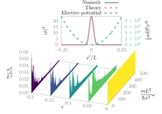
Figure 1: Dynamical trapping produced by the breathing of two impenetrable walls. (a) The numerically computed variance of the Floquet eigenstate with the lowest variance as a function of $\omega$ and $\epsilon$. (b) Comparison between the lowest variance Floquet eigenstate and the ground state predicted by the average harmonic oscillator potential trap, and the corresponding effective potential produced by the breathing of the system for $\omega=5,000\,\hbar\pi^{2}m^{-1}L^{-2}$, and $\epsilon=0.05$. The numerical calculation was performed up to $N=30$ eigenstates of the static problem.

First, and for the sake of illustration (both numerical and analytical) let’s show the stabilization effect and the validity of our approximation assuming that the potential is the one given by two impenetrable walls at $x=-L/2$ and $x=L/2$, and we proceed to solve the lowest variance Floquet eigenstate. The Floquet eigenstates $\phi^{(\mu)}$ and the quasi-energies or Floquet exponents $\mu$ are defined as the solutions of Eq. (4) of the form $\phi^{(\mu)}(z^{\prime}+T)=\phi^{(\mu)}(z^{\prime})\,\exp(-i\mu T)$. uch states are calculated expanding and projecting $\phi$ in the eigenfunctions $\phi_{n}$ of the static case ($\epsilon=0$), namely, $\phi=\alpha^{-1/2}\sum_{n=1}^{\infty}a_{n}\phi_{n}$, and truncating the sum up to $N$ to obtain system of ordinary differential equations. The factor $\alpha^{-1/2}$ should be added in order to preserve normalization. In Fig. 1 we observe the dynamical trapping produced by the breathing waveguide. This is revealed by Fig. 1(a), where we see the numerically calculated values of $\sigma_{x}^{2}$, the variance in the coordinate $x$ of the light envelope, for the Floquet eigenstate, with the lowest variance, as a function of $\epsilon$ and $\omega$. Note that generally, the envelope becomes more localized as $\epsilon$ and $\omega$ grows, as it has been predicted by the Eq. (4). However, we can observe some exceptions as peaks of $\sigma_{x}^{2}$ for certain spatial frequencies. These peaks are associated with resonant behavior between the normal modes of the static system. In such case, a lowest variance Floquet eigenstate is expected to be a linear combination of some of such modes that include the resonant one, and so is likely to be an unlocalized state. However, such effects are more clearly observed at low frequencies because the resonance region becomes much thinner as the difference of frequencies becomes larger (see Ref. Carrasco et al. (2017)). Even more, we can conclude that it is more likely to encounter the system localized because such exceptions only occur at very specific frequencies, and so the effect is very robust. In Fig. 1(b) we show the lowest variance Floquet eigenstate of the full Eq. (2), at $\omega=25\,\hbar\pi^{2}m^{-1}L^{-2}$ and $\epsilon=0.05$, and the one predicted by Eq. (4), and the corresponding effective harmonic oscillator potential trap produced by the breathing of the system. As we can see, our approximation agrees quite closely with the exact solution, even for not too large spatial frequencies (tens of times the frequency of the lowest mode of the non breathing impenetrable walls). Summing up, we found the predicted trapping effect, which is still present at relatively low spatial frequencies, but may be destroyed by resonances with the Rabi oscillations between the static modes.

Now we turn to another important objective of this work, namely, to show how breathing lattice can trap light beams where non-breathing lattices cannot. Let us consider light propagating in a waveguide which is breathing in the perpendicular direction $x$, and propagates along the parallel direction $z$. The time evolution of a complex beam envelope function $\psi(x,z)$ follows an optical analog of the Schrödinger equation, and so following the same arguments presented above, the optical equivalent of the Eq. (2) with $m$ exchanged for $n_{s}$, $t^{\prime}$ for $z^{\prime}$, and $\hbar$ for $\lambdabar$ is

$$i\lambdabar\frac{\partial\phi}{\partial z^{\prime}}=-\frac{\lambdabar^{2}}{2n_{s}\alpha^{2}}\frac{\partial^{2}\phi}{\partial x^{\prime 2}}+\frac{V(x^{\prime})}{\alpha^{2}}\phi-\left(\frac{1}{2}\alpha\ddot{\alpha}+\dot{\alpha}^{2}\right)n_{s}x^{\prime 2}\phi\ ,$$ (5)

where $z^{\prime}$ is the paraxial propagation distance, $x^{\prime}$ now is the spatial position in the non-breathing frame, $\lambdabar=\lambda/(2\pi)$ is the reduced wavelength, $V(x)=n_{s}-n(x)$, $n(x)$ is the effective refractive index profile of the array, $n_{s}$ is the bulk refractive index, and $\alpha=\alpha(z)$ describes the breathing of the waveguide. Now let us consider a breathing waveguide lattice, which in the standard nearest-neighbor tight-binding approximation is governed by a discrete version of Eq. (4) (see Appendix), namely

$$i\dot{c}_{n}=-\frac{k}{\alpha}(c_{n+1}+c_{n-1})+i\frac{\dot{\alpha}}{\alpha}c_{n}-\left(\frac{1}{2}\alpha\ddot{\alpha}+\dot{\alpha}^{2}\right)\frac{n_{s}a^{2}n^{2}}{\lambdabar}c_{n}\ ,$$ (6)

where $k$ is the coupling constant between adjacent waveguides, $a$ the distance between adjacent waveguides in the non-breathing case, and $c_{n}$ the mode amplitude. Fig. 2 shows the propagation of a Gaussian beam obtained by direct numerical simulations of Eq. (6) with $\alpha(z)=1+\epsilon\cos(\omega z)$, as it was chosen for the previous calculations. It worth to recall that the no singularity condition ($|\epsilon|<1$) keeps the distances between two points always greater than zero, hence two waveguides never touch each other. The initial condition is set as $c_{n}(0)=\exp(-n^{2}/5)$. In Fig. 2(a) we observe the propagation through a non-breathing ($\epsilon=0$) waveguide lattice which acts as a defocusing lens for the discretized beam. In Fig. 2(b) we observe the dynamic trapping of the beam as it travels through the breathing waveguide with $\epsilon=0.1$, $\omega=k$, and $n_{s}a^{2}\lambdabar^{-1}k=1$, which is very close of to the experimental case, considering that the typical experimental values, namely $a$ of the order of $10\,\mu\text{m}$, $\lambdabar$ of the order of $100\,\text{nm}$, $n_{s}$ around unity, and $k$ of the order of $\text{mm}^{-1}$ Longhi (2005b); Longhi et al. (2006); Weimann et al. (2018). Indeed, for this typical coupling constant $k$ is of the order of a $\text{mm}^{-1}$, and the propagation length shown on Fig. 2 corresponds to a physical length which is of the order of 1 cm. Remarkably, the effect which was illustrated for the impenetrable wall problem at high frequencies persists even for relatively small spatial modulation frequencies (of the order of the coupling constant $k$), opening the possibility to observe this trapping effect with the current experimental capabilities.

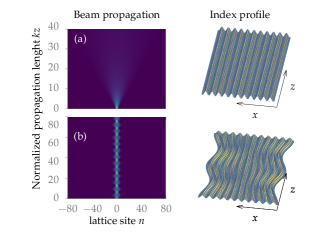
Figure 2: Beam propagation (snapshot of $|c_{n}(z)|^{2}$) in a breathing lattice with $\omega=k$ for (a) $\epsilon=0$ and (b) $\epsilon=0.1$. The right panels schematically show the index profile of the non-breathing (upper plot) and breathing (lower plot) waveguide array.

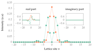
Figure 3: Numerically computed intensity distribution $|c_{n}^{2}|$ for the two most localized metastable states (Floquet eigenstates), at the plane $z=0$, for the breathing waveguide lattice with $\omega=k$ and $\epsilon=0.1$. The insets show the real and imaginary parts of the states.

This trapping effect is related to the existence of a Floquet eigenstate (metastable state) which is similar to the initial condition, or a sort of an effective potential produced by the breathing of the system, as it was discussed before for an arbitrary potential. For the parameters of the breathing waveguide used in Fig. 2(b), the Floquet eigenstates can be numerically calculated. Assuming an array of 161 waveguides, in Fig. 3 we observe the two most localized states. It’s interesting to note that the most localized metastable state highly resembles the initial condition used in Fig. 2(b), and then explain why it remains trapped around the lattice site $n=0$ while it travels along the propagation axis $z$.

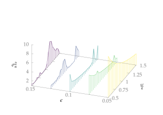
Figure 4: Numerically computed lowest variance of all Floquet eigenstates in the waveguide lattice as a function of $\omega$ and $\epsilon$.

In a similar way that it was done before for the case of two impenetrable walls, in Fig. 4 we see the numerically calculated values of $\sigma_{n}^{2}=\sum_{n}n^{2}c_{n}^{2}$, the variance in the lattice site $n$ of the mode amplitude, and plotted the lowest variance among all Floquet eigenstates as a function of $\epsilon$ and $\omega$. We observe that the behavior of the waveguide lattice strongly resembles the behavior of the system of two impenetrable walls, and so the localization grows as we increase the value of the breathing amplitude $\epsilon$ and the spatial frequency $\omega$. However, this doesn’t hold for certain frequencies and values of $\epsilon$ which, as it was stated before, may correspond to a Rabi-like behavior of the system. As a final remark, we must state that this show again that the effect persist even for relatively small spatial modulation frequencies.

In conclusion, a new scheme of dynamical stabilization is presented, in a way that is directly based in the simulation of a Paul trap Goldman and Dalibard (2014) using a harmonically breathing potential at high frequency. Using this approach it’s possible to trap light wherever is desired, and such capability remains even for relatively small breathing frequencies. Even more, such trapping allows us to simulate potentials that may go beyond the static experimental capabilities. Finally, it must be stated that this particle trapping strategy analogy is not limited to quantum particles and light, it can be applied to any system that follows a Schrödinger-like equation, and so it can be used equally to trap other kinds of bosons and fermions.

The authors are pleased to acknowledge M. Clerc for a valuable discussion about stabilization effects. This work was supported by CONICYT-PCHA/Doctorado Nacional/2016-2116103 (S.C.) and the Fondo Nacional de Investigaciones Científicas y Tecnológicas (FONDECYT, Chile) under grants #1160639 (JR), #1150718 (JAV), and CEDENNA through “Financiamiento Basal para Centros Científicos y Tecnológicos de Excelencia-FB0807” (JR and JAV). We also acknowledge support from Grant FA9550-18-1-0438 of the U.S.A.F. Office of Scientific Research (JR and JAV).

Appendix.—In the tight-binding approximation

$$\phi=\sum_{n}c_{n}u_{n}\left(x\right)\ ,$$ (7)

where $u_{n}(x)=u(x-na)$ is a localized mode in the lattice site $n$. It is reazonable to assume that the localized mode is Gaussian, namely

$$u(x)=\frac{1}{(2\pi b^{2})^{1/4}}\exp\left(-\frac{x^{2}}{4b^{2}}\right)\ .$$

In the nearest-neighbor approximation

$$\int H_{0}u_{n}u_{m}\,dx\approx e\delta_{n,m}-\lambdabar k\delta_{n,m+1}\ ,$$

where $H_{0}$ is the Hamiltonian in the non-breathing case, $e$ the energy of the localized mode, and $k>0$ is the coupling constant between adjacent waveguides. It will be usefull to use the fact that in the nearest-neighbor approximation

$$\int x^{2}u_{n}u_{m}\,dx\approx n^{2}a^{2}\delta_{n,m}\ .$$

Now let’s turn to the breathing case. The time evolution follows Eq (5), namely

$$i\lambdabar\frac{\partial\phi}{\partial z^{\prime}}=\frac{1}{\alpha}H_{0}\phi-\left(\frac{1}{2}\alpha\ddot{\alpha}+\dot{\alpha}^{2}\right)n_{s}x^{\prime 2}\phi\ .$$ (8)

In the non-breathing frame Eq. (7) should be rewritten as

$$\phi=\sum_{n}\sqrt{\frac{1}{\alpha}}c_{n}u_{n}\left(x^{\prime}\right)\ .$$

Note that a factor $\sqrt{1/\alpha}$ should be added to preserve the normalization. Reeplacing this back on (8) and projecting, gives

$$i\dot{c}_{n}=-\frac{k}{\alpha}(c_{n+1}+c_{n-1})+i\frac{\dot{\alpha}}{\alpha}c_{n}+\frac{e}{\alpha}c_{n}\\ -\left(\frac{1}{2}\alpha\ddot{\alpha}+\dot{\alpha}^{2}\right)\frac{n_{s}a^{2}n^{2}}{\lambdabar}c_{n}\ .$$

Making the cannonical transformation $c^{\prime}_{n}=c_{n}\exp\left(-ie\int\limits_{0}^{z}\frac{dz^{\prime}}{\alpha(z^{\prime})}\right)$ we obtain Eq. (6), namely,

$$i\dot{c}_{n}=-\frac{k}{\alpha}(c_{n+1}+c_{n-1})+i\frac{\dot{\alpha}}{\alpha}c_{n}-\left(\frac{1}{2}\alpha\ddot{\alpha}+\dot{\alpha}^{2}\right)\frac{n_{s}a^{2}n^{2}}{\lambdabar}c_{n}\ .$$

References

- Rechtsman et al. (2013) M. C. Rechtsman, J. M. Zeuner, Y. Plotnik, Y. Lumer, D. Podolsky, F. Dreisow, S. Nolte, M. Segev, and A. Szameit, Nature 496, 196 (2013).
- Polini et al. (2013) M. Polini, F. Guinea, M. Lewenstein, H. C. Manoharan, and V. Pellegrini, Nature nanotechnology 8, 625 (2013).
- Jacqmin et al. (2014) T. Jacqmin, I. Carusotto, I. Sagnes, M. Abbarchi, D. Solnyshkov, G. Malpuech, E. Galopin, A. Lemaître, J. Bloch, and A. Amo, Physical review letters 112, 116402 (2014).
- Dalibard et al. (2011) J. Dalibard, F. Gerbier, G. Juzeliūnas, and P. Öhberg, Reviews of Modern Physics 83, 1523 (2011).
- Zhai (2012) H. Zhai, International Journal of Modern Physics B 26, 1230001 (2012).
- Longhi et al. (2006) S. Longhi, M. Marangoni, M. Lobino, R. Ramponi, P. Laporta, E. Cianci, and V. Foglietti, Physical review letters 96, 243901 (2006).
- Szameit et al. (2010) A. Szameit, I. L. Garanovich, M. Heinrich, A. A. Sukhorukov, F. Dreisow, T. Pertsch, S. Nolte, A. Tünnermann, S. Longhi, and Y. S. Kivshar, Physical review letters 104, 223903 (2010).
- Longhi (2015) S. Longhi, Optics letters 40, 4707 (2015).
- Longhi (2005a) S. Longhi, Physical Review A 71, 065801 (2005a).
- Della Valle et al. (2007) G. Della Valle, M. Ornigotti, E. Cianci, V. Foglietti, P. Laporta, and S. Longhi, Physical review letters 98, 263601 (2007).
- Szameit et al. (2009) A. Szameit, Y. V. Kartashov, F. Dreisow, M. Heinrich, T. Pertsch, S. Nolte, A. Tünnermann, V. A. Vysloukh, F. Lederer, and L. Torner, Physical review letters 102, 153901 (2009).
- Mukherjee et al. (2016) S. Mukherjee, M. Valiente, N. Goldman, A. Spracklen, E. Andersson, P. Öhberg, and R. R. Thomson, Physical Review A 94, 053853 (2016).
- Luo et al. (2007) X. Luo, Q. Xie, and B. Wu, Physical Review A 76, 051802 (2007).
- Ornigotti et al. (2008) M. Ornigotti, G. Della Valle, T. T. Fernandez, A. Coppa, V. Foglietti, P. Laporta, and S. Longhi, Journal of Physics B: Atomic, Molecular and Optical Physics 41, 085402 (2008).
- Kartashov et al. (2007) Y. V. Kartashov, V. A. Vysloukh, and L. Torner, Phys. Rev. Lett. 99, 233903 (2007).
- Shandarova et al. (2009) K. Shandarova, C. E. Rüter, D. Kip, K. G. Makris, D. N. Christodoulides, O. Peleg, and M. Segev, Phys. Rev. Lett. 102, 123905 (2009).
- Schwartz (2007) T. Schwartz, Nature (London) 446, 52 (2007).
- Wiersma et al. (1997) D. S. Wiersma, P. Bartolini, A. Lagendijk, and R. Righini, Nature 390, 671 (1997).
- Lahini et al. (2008) Y. Lahini, A. Avidan, F. Pozzi, M. Sorel, R. Morandotti, D. N. Christodoulides, and Y. Silberberg, Physical Review Letters 100, 013906 (2008).
- Wolf and Maret (1985) P.-E. Wolf and G. Maret, Physical review letters 55, 2696 (1985).
- Van Albada and Lagendijk (1985) M. P. Van Albada and A. Lagendijk, Physical review letters 55, 2692 (1985).
- John (1984) S. John, Physical Review Letters 53, 2169 (1984).
- Theocharis et al. (2006) G. Theocharis, P. Schmelcher, P. Kevrekidis, and D. Frantzeskakis, Physical Review A 74, 053614 (2006).
- Longhi (2011) S. Longhi, Optics letters 36, 819 (2011).
- Papagiannis et al. (2011) P. Papagiannis, Y. Kominis, and K. Hizanidis, Physical Review A 84, 013820 (2011).
- Longhi (2005b) S. Longhi, Optics letters 30, 2137 (2005b).
- Iyer et al. (2007) R. Iyer, J. S. Aitchison, J. Wan, M. M. Dignam, and C. M. de Sterke, Optics express 15, 3212 (2007).
- Earnshaw (1842) S. Earnshaw, Trans. Camb. Phil. Soc. 7, 97 (1842).
- Goldman and Dalibard (2014) N. Goldman and J. Dalibard, Physical review X 4, 031027 (2014).
- Cook et al. (1985) R. J. Cook, D. G. Shankland, and A. L. Wells, Physical Review A 31, 564 (1985).
- Gilary et al. (2003) I. Gilary, N. Moiseyev, S. Rahav, and S. Fishman, Journal of Physics A: Mathematical and General 36, L409 (2003).
- Carrasco et al. (2017) S. Carrasco, J. Rogan, and J. A. Valdivia, Scientific reports 7, 13217 (2017).
- Weimann et al. (2018) S. Weimann, T. Eichelkraut, and A. Szameit, Physical Review A 97, 053844 (2018).