A global algorithm for the computation of traveling dissipative solitons

Abstract

An algorithm is proposed to calculate traveling dissipative solitons for the FitzHugh-Nagumo equations. It is based on the application of the steepest descent method to a certain functional. This approach can be used to find solitons whenever the problem has a variational structure. Since the method seeks the lowest energy configuration, it has robust performance qualities. It is global in nature, so that initial guesses for both the pulse profile and the wave speed can be quite different from the correct solution. Also, bifurcations have a minimal effect on the performance. With an appropriate set of physical parameters in two dimensional domains, we observe the co-existence of single-soliton and 2-soliton solutions together with additional unstable traveling pulses. The algorithm automatically calculates these various pulses as the energy minimizers at different wave speeds. In addition to finding individual solutions, this approach could be used to augment or initiate continuation algorithms.

1 Introduction

Patterns occurring in nature fascinate. They are ubiquitous in all kinds of physical, chemical and biological systems. Very often, localized structures are observed, like pulses, fronts and spirals. These fundamental building blocks then self-organize into patterns as a result of their mutual interaction. This may involve a pattern front moving across a homogeneous ambient state after some kind of destabilization. In many cases, the ambient state is uniform in all directions. Traveling pulses are localized structures which relax to the same ambient state; they are therefore especially important in the dynamic transition phase seen in many experiments and model simulations. Stable pulses (which are sometimes called spots in multidimensional domains), whether stationary or moving, can be particle-like in many circumstances and are often referred to as dissipative solitons in the physics literature. For example, see the books by Nishiura (2002); Akhmediev and Ankiewicz (2005); Liehr (2013) and the references therein. In a three-component activator-inhibitor system studied by both physicists and mathematicians, it was observed that fast moving solitons collide to annihilate one another while slow ones bounce off from one another, and an unstable standing pulse can split into two solitons; see Purwins et al. (2005); Ei et al. (2006); Kawaguchi and Mimura (2008); Nishiura et al. (2007); van Heijster et al. (2010).

Understanding the mechanisms behind such pattern formation has been an on-going struggle since Turing’s landmark paper on morphogenesis, Turing (1952); investigation has intensified in the last three decades in recognition of the importance observed for various applications. Advances in mathematical studies lead to a deeper understanding: such interactions involve a delicate balance between gain and loss, and the subsequent redistribution of energy and “mass” in the system; the “mass” can be chemical concentration, light intensity or current density. Many dissipative soliton models, like Ginsburg-Landau and nonlinear Schrodinger equations, possess variational structures. Restricting our attention to reaction-diffusion systems, activator-inhibitor type equations are the natural choices in modeling these phenomena, as they involve gain and loss; see Purwins et al. (2005); Liehr (2013). The two component FitzHugh-Nagumo equations and the three component activator-inhibitor systems serve as primary models in such investigations; under suitable parametric restrictions the solutions are minimizers of some variational functionals.

There are many theoretical studies on these activator-inhibitor systems that employ various methods of analysis for one or higher dimensional domains in different parametric regimes, for example Chen and Choi (2012, 2015); Chen et al. (2016); van Heijster and Sandstede (2014); Muratov (2004); Dancer et al. (2007); Ren and Wei (2003). We are particularly interested in the case when the activator diffusivity is small (compared to that of the inhibitor), leading to an activator profile with a steep slope. By using the tool of $\Gamma$-convergence on the FitzHugh-Nagumo equations to study its limiting geometric variational problems with a nonlocal term, existence and local stability of radially symmetric standing spots in ${\mathbb{R}}^{n}$ have been completely classified for all parameters Chen et al. (2018b, a); they are the first results on the exact multiplicity of solutions to these limiting equations (from $0$ up to $3$ standing pulses). With similar restrictions on parameters in order to employ $\Gamma$-convergence, a unique traveling pulse solution in the 1D case has also been shown recently Chen et al. . However, when we relax the conditions on the parameters (so that one cannot employ $\Gamma$-convergence analysis), there can be co-existence of a traveling pulse and two distinct fronts moving in opposite directions Chen and Choi (2018).

Computational studies are also important, but there can be difficulties. Continuation algorithms are a common means to compute traveling and stationary waves. While there is no difficulty in finding 1D traveling spots of the FitzHugh-Nagumo equations, the 2D case is different. We extract an exact quote from (Liehr, 2013, p.8): “Only in extreme parameter regimes, where numerical solutions are difficult to obtain, it can be analytically shown that propagating dissipative solitons exist as stable solutions of two-component, two- dimensional, reaction-diffusion systems”; the algorithms experience a hindrance. At the same time, from (Ei et al., 2006, bottom of p.32): “it is generally believed that traveling spots for a two component system in the whole $\mathbb{R}^{2}$ do not exist”. The difficulty comes as a result of multiple bifurcations in the 2D domains. Sometimes, just in some small range of parameters there are multiple bifurcations occurring (the cusp in Figure 6 is related to bifurcation), resulting in many close-by solutions; in such situations it is not easy to find a good enough initial guess for the continuation algorithm. Even when sucessful, convergence is not guaranteed.

Another computational approach is to feed reasonable initial profiles into the time dependent problem and perform numerical time stepping; one then hopes that it results in a more or less steady profile moving at a uniform speed after a long run. All unstable waves can never be found using such a method. Even if a stable traveling wave exists, it is easy to miss the solution since usually they are not global attractors for reaction-diffusion systems, as in the case of the FitzHugh-Nagumo equations. This method sometimes provides a good initial guess for a Newton-type algorithm or a numerical shooting method if we are interested in very accurate solutions. As we are interested in cases when $d$ is small, the resulting multiple temporal and spatial scales in (1) will induce excessive computational effort, unless the initial approximation is extremely good so that the convergence to the traveling wave takes place in a short time.

If we restrict ourselves to dissipative solitons for which variational formulations are common, we may exploit the fact that they are minimizers. In this paper, we develop a robust, global steepest descent algorithm to find traveling pulse solutions of the FitzHugh-Nagumo equations both in 1D and on an infinite strip domain in 2D with zero Dirichlet boundary conditions. It is based on some recent theoretical understanding; see Chen and Choi (2012, 2015). The algorithm works even without a good initial guess. If a bifurcation occurs, it simply tracks the lowest energy configuration and filters out other high energy solutions generated as a result of bifurcation. Multiple bifurcations in a vicinity will therefore not affect the algorithmic performance. That explains why we are able to find quite a few stable and unstable spots with relative ease in our computations. Future robustness tests on this algorithm will be conducted with other boundary conditions, widening the width of the strip domain, and for traveling fronts. Another study Choi et al. also shows that the algorithm can easily compute all three traveling waves proved in Chen and Choi (2018); in fact, in addition to these 3 stable minimizers there are 2 unstable waves with the same physical parameters. The algorithm can also be applied toward the 3-component activator-inhibitor systems, which also possess variational structures.

We consider the FitzHugh-Nagumo equations with domain $\Omega\subset\mathbb{R}^{n}$ in space, for time $0\leq t<\infty$. Specifically, $\Omega=\mathbb{R}$ if $n=1$ and $\Omega=\mathbb{R}\times(-L,L)$ if $n=2$, with $0<L<\infty$. The equations are:

$$\begin{array}[]{rl}\displaystyle u_{t}&=\displaystyle\Delta u+\frac{1}{d}\left(f(u)-v\right),\\ \displaystyle v_{t}&=\displaystyle\Delta v+u-\gamma\,v,\end{array}$$ (1)

plus initial conditions. Boundary conditions are needed for $n=2$; we consider $u=v=0$ on the boundary. Here $d$ and $\gamma$ are positive constants, and $f(u)\equiv u(u-\beta)(1-u)$ with $0<\beta<1/2$ being a fixed constant.

Our algorithm is global in the sense that it does not require a good initial guess of the solution, only some guess in the set ${\mathcal{A}}$ that we show later is very easy to construct. The wave speed is found as a root of a certain functional. Multiple roots correspond to distinct waves, hence multiple solutions for the same values of $d$, $\gamma$ and $\beta$. We develop this approach here for the specific domains $\Omega$ described above, but it can be easily extended to more general boundary conditions and domains via standard adaptations of the variational techniques. After deriving our method, we will computationally illustrate how it is used to determine the existence and multiplicity of traveling pulse solutions to (1), and simultaneously compute the corresponding wave speeds and pulse profiles. In 2D, we observe a bifurcation and point out how the energy minimization property allows the algorithm to adapt automatically and find the dissipative soliton.

1.1 An illustration of robustness

As an example of the global convergence with $n=1$, choosing $\beta=1/4$, $d=0.0005$ and $\gamma=1/16$, our proposed method is able to identify one stable and one unstable wave profile, corresponding to different wave speeds $c_{0}$ and $c_{1}$, respectively. In order to check the stability of our computed traveling pulses, they are input as initial data into a parabolic solver for the time-dependent equation (1). While some break up quickly, which indicates an unstable traveling wave; others just translate with the computed speed from our descent algorithm, verifying that they are stable.

The situation is illustrated in Figure 1; on the top, we show the result of inserting the unstable traveling wave profile into a parabolic solver: the wave just decays rapidly in time. This demonstates the need of a global algorithm; if the initial guess for a stable wave profile is not close enough, the parabolic solver may not find it. In contrast, our proposed method can start with the same unstable profile and be used to find the stable profile with speed $c_{0}$ as well. In the center of Figure 1, this process is shown at various iteration counts, $n$, of the algorithm. On the bottom of Figure 1, we show the result of inserting the computed, stable wave profile into the parabolic solver.

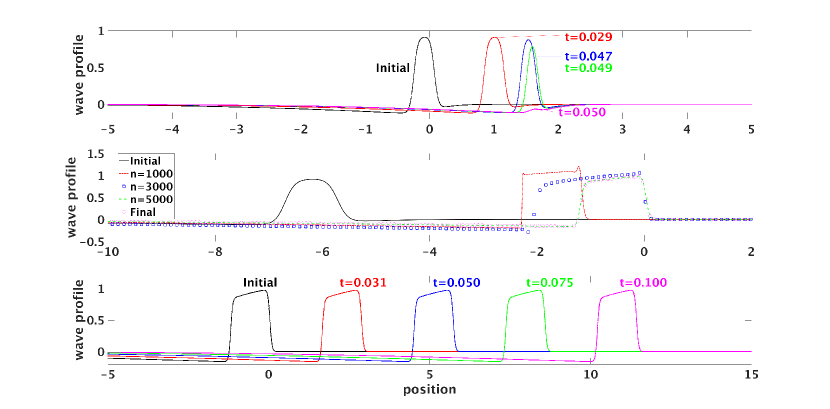
Figure 1: Top: an initial guess for a traveling wave profile that decays rapidly in a parabolic solver. Center: the same initial guess is used to initiate the proposed global method (after a change of variables, described later). Snapshots are shown for various iteration counts, $n$. Bottom: the resulting profile now remains steady in a parabolic solver.

The remainder of this paper is organized as follows. In Section 2 we give a variational formulation of the FitzHugh-Nagumo equations so that a critical point corresponds to a traveling pulse, provided its wave speed also satisfies an auxiliary scalar algebraic equation. The admissible set ${\mathcal{A}}$ in which we look for the critical point has to be described carefully. In Section 3 we present a steepest descent algorithm which, together with the auxiliary scalar algebraic equation, computes a traveling pulse profile as well as its wave speed. The details in Section 2-Section 3 are presented for one dimension of space. In Section 4, we explain the extension to two dimensions, which requires fairly minor modifications that are standard for variational analyses. In Section 5 we present, compare and perform some checks on numerical results from our algorithm in one dimension of space. The fastest traveling pulse speed has an asymptotic limit as $d\to 0$, see Chen and Choi (2015); we check our numerical wave speed against this theoretical result and find excellent agreement. In Section 6 we present numerical results for two-dimensional domains and find as many as four traveling pulse solutions (with different wave speeds) for a single choice of parameters. A bifurcation separates these pulses into two distinct groups qualitatively, but the algorithm automatically computes them all without any special or prior knowledge of the pulse profiles. In Section 7 we give a short summary of our results and discuss some future work. In the remainder of this paper, the terminologies ‘pulse’, ‘spot’ and ‘dissipative soliton’ essentially mean the same thing. We use ‘pulse’ in 1D to conform to mathematicians’ preference. In 2D, if the pulse is stable, we call it a (dissipative) soliton to emphasize its localized structure with a particle-like property.

2 A variational formulation for traveling pulse

In this section we take $n=1$ for (1); the case $n=2$ is handled in Section 4. Following (Chen and Choi, 2015, Theorems 1.1) we impose the restriction $0<\gamma<4/(1-\beta)^{2}$. This is a necessary and sufficient condition for the straight line $u=\gamma v$ to cut the curve $v=f(u)$ only at the origin in the $(u,v)$ plane. This guarantees that $(u,v)=(0,0)$ is the only constant-state equilibrium solution and hence eliminates the possibility of a traveling front. Under such a condition the cited Theorem 1.1 ensures that a traveling pulse solution exists when $d$ is sufficiently small with fixed $\gamma$ and $\beta$.

We look for traveling pulse solutions $(u(x,t),v(x,t))\in\mathbb{R}^{2}$ of (1) with $-\infty<x<\infty$ and $t\geq 0$. For a wave speed $c$, which is not yet known, we require that

$$u(x,t)=\tilde{u}(c(x-ct))\ \ \text{and}\ \ v(x,t)=\tilde{v}(c(x-ct))$$ (2)

for some smooth functions $\tilde{u}:{\mathbb{R}}\to{\mathbb{R}}$ and $\tilde{v}:{\mathbb{R}}\to{\mathbb{R}}$. Dropping the tilde in the notation and use $x$ to denote $\xi=c(x-ct)$, the traveling pulse problem is to find $(u,v,c)$ satisfying

$$\begin{array}[]{rl}\displaystyle dc^{2}\frac{\partial^{2}{u}}{\partial x^{2}}+dc^{2}\frac{\partial{u}}{\partial x}+f(u)-v&=0,\\ \displaystyle c^{2}\frac{\partial^{2}{v}}{\partial x^{2}}+c^{2}\frac{\partial{v}}{\partial x}+u-\gamma\,v&=0\end{array}$$ (3)

with $(u,v)\to(0,0)$ as $|x|\to\infty$. We can always let $c>0$.

We introduce Hilbert spaces ${L^{2}_{ex}}({\mathbb{R}})$ and ${H^{1}_{ex}}({\mathbb{R}})$, corresponding to the inner products

$$\langle v,w\rangle_{{L^{2}_{ex}}} \equiv\int_{\mathbb{R}}e^{x}vw\,dx$$ (4)

$$\text{and}\ \ \langle v,w\rangle_{{H^{1}_{ex}}} \equiv\int_{\mathbb{R}}e^{x}\left\{\frac{\partial{v}}{\partial x}\frac{\partial{w}}{\partial x}+vw\right\}\,dx,$$

respectively. The induced norms are denoted by $\|\cdot\|_{{L^{2}_{ex}}}$ and $\|\cdot\|_{{H^{1}_{ex}}}$. A variational approach will be used to find weak solutions $(u,v)\in({H^{1}_{ex}})^{2}$ to  (3).

By solving (3b) we write $v={\mathcal{L}_{c}}u$, where ${\mathcal{L}_{c}}:{L^{2}_{ex}}\to{L^{2}_{ex}}$ is a linear operator. It can be verified that ${\mathcal{L}_{c}}$ is a self-adjoint operator on ${L^{2}_{ex}}({\mathbb{R}})$, i.e. $\langle u_{1},{\mathcal{L}_{c}}u_{2}\rangle_{{L^{2}_{ex}}}=\langle{\mathcal{L}_{c}}u_{1},u_{2}\rangle_{{L^{2}_{ex}}}$ for any $u_{1},u_{2}\in{L^{2}_{ex}}({\mathbb{R}})$. A way to see this is to write (3b) as $c^{2}(e^{x}v_{i}^{\prime})^{\prime}-\gamma e^{x}v_{i}=-e^{x}u_{i}$ for $i=1,2$; then it is easy to check $\langle u_{1},v_{2}\rangle_{{L^{2}_{ex}}}=\langle v_{1},u_{2}\rangle_{{L^{2}_{ex}}}$, provided there is sufficient control on $u_{i}$ and $v_{i}$ so that the boundary terms at infinity arising from integration by parts can be discarded.

For any given $c>0$, consider the functional $J_{c}:{H^{1}_{ex}}\to\mathbb{R}$ defined by

$$J_{c}(w)\equiv\int_{\mathbb{R}}e^{x}\left\{\frac{dc^{2}}{2}w^{\prime\,2}+\frac{1}{2}w\,{\mathcal{L}_{c}}w+{\mathcal{F}}(w)\right\}\,dx,$$ (5)

where

$${\mathcal{F}}(\xi)=-\int_{0}^{\xi}f(\tau)\,d\tau=\frac{\xi^{4}}{4}-\frac{(1+\beta)\xi^{3}}{3}+\beta\frac{\xi^{2}}{2}.$$ (6)

Making use of the self-adjointness of ${\mathcal{L}_{c}}$ on ${L^{2}_{ex}}({\mathbb{R}})$, its Fréchet derivative is given by

$$J_{c}^{\prime}(w)\phi\equiv\int_{\mathbb{R}}e^{x}\left\{dc^{2}w^{\prime}\,\phi^{\prime}+{\mathcal{L}_{c}}w\,\phi-f(w)\phi\right\}\,dx\ \ \ \text{for all}\ w,\phi\in{H^{1}_{ex}}({\mathbb{R}}).$$ (7)

A critical point $u$ of $J_{c}$ in ${H^{1}_{ex}}({\mathbb{R}})$ will satisfy the Euler-Lagrange equation associated with $J_{c}$, namely

$$-dc^{2}(e^{x}u^{\prime})^{\prime}-e^{x}f(u)+e^{x}{\mathcal{L}_{c}}u=0\;.$$ (8)

This integral-differential equation is equivalent to the Fitzhugh-Nagumo equations (3). Recall that ${H^{1}_{ex}}({\mathbb{R}})\subset C({\mathbb{R}})$, we are now ready for the following.

Definition 1

A function $w\in C(\mathbb{R})$ is in the class ${-/+/-}$ if there exist $-\infty\leq x_{1}\leq x_{2}\leq\infty$ such that (a) $w(x)\leq 0$ for all $x\in(-\infty,x_{1}]\cup[x_{2},\infty)$ and (b) $w(x)\geq 0$ for all $x\in[x_{1},x_{2}]$.

Remark 1

(a) In the above definition, the choice of $x_{1},x_{2}$ is not necessarily unique. If $x_{1}=-\infty$ and $x_{2}=\infty$, then $w\geq 0$ on the real line. In case $x_{1}=x_{2}=\infty$, then $w\leq 0$ on the real line. Both examples are included in the class $-/+/-$.
(b) A function $w$ is said to change sign twice, if $w\leq 0$ on $(-\infty,x_{1}]\cup[x_{2},\infty)$, $w\geq 0$ on $(x_{1},x_{2})$ and $w\not\equiv 0$ in each of such three intervals.

As $\beta<1/2$, there is a unique $\beta_{1}$ such that $\beta<\beta_{1}<1$ with ${\mathcal{F}}(\beta_{1})=0$. In addition, we take a constant $M_{1}=M_{1}(\gamma)\geq 1$ such that $f(\xi)\geq 1/\gamma$ for all $\xi\leq-M_{1}$. A class ${\mathcal{A}}$ of admissible functions to be employed in the variational argument is defined as follows.

Definition 2

$${\mathcal{A}}\equiv\left\{w\in{H^{1}_{ex}}:\|w\|_{{H^{1}_{ex}}}^{2}=2,\,-M_{1}\leq w\leq 1,w\;\mbox{is in the class}\;{-/+/-}\right\}.$$ (9)

We restrict attention to $J_{c}:{\mathcal{A}}\to{\mathbb{R}}$. A global minimizer is known to exist in ${\mathcal{A}}$ for any fixed $c>0$. We can therefore let

$${\mathcal{J}(c)}\equiv\min_{w\in{\mathcal{A}}}J_{c}(w),\ \ \text{for all}\ c>0.$$ (10)

When $d\leq d_{0}$ for some sufficiently small $d_{0}$, it can be shown that ${\mathcal{J}(c)}<0$ when $c$ is small, ${\mathcal{J}(c)}>0$ when $c$ is large, and $\cal J$ is a continuous function. By the intermediate value theorem there is at least one $c_{0}>0$ such that $\mathcal{J}(c_{0})=0$. Suppose $u_{0}$ is a global minimizer in ${\mathcal{A}}$ when $c=c_{0}$, and we let $v_{0}={\cal L}_{c_{0}}u_{0}$, then $(u_{0},v_{0})$ can be shown to be smooth and $(u_{0},v_{0},c_{0})$ is a traveling pulse solution; thus $u_{0}$ is an unconstrained critical point of $J_{c_{0}}$. We will give a heuristic argument in subsection 2.1 on why ${\mathcal{J}(c)}=0$ determines the wave speed. The rigorous proof is in Chen and Choi (2015).

For any fixed $c$ we will construct a steepest descent algorithm in the next section to find ${\mathcal{J}(c)}$ and the corresponding minimizer $u$ of $J_{c}$. A spatial translation of any traveling pulse solution remains a traveling pulse. This continuum of solutions will induce both theoretical and numerical difficulties. The condition $\|u_{0}\|_{{H^{1}_{ex}}}^{2}=2$ in ${\mathcal{A}}$ makes sure that $u_{0}(\cdot+a)$ is not in ${\mathcal{A}}$ for any non-zero $a\in{\mathbb{R}}$ and hence eliminates translation of solution.

Remark 2

The admissible set ${\mathcal{A}}$ defined above differs slightly from that in (2.9) of Chen and Choi (2015), because

1. the weighted $H^{1}$ norm $\|w\|_{{H^{1}_{ex}}}$ employed here is equivalent to the norm $\sqrt{\int_{\mathbb{R}}e^{x}w_{x}^{2}\,dx}$ used in Chen and Choi (2015). The new norm may be better when we perform numerical computations after truncating the real line to a finite domain.

2. Subsequent analysis in Chen and Choi (2015) leads to tighter bounds on a local minimizer of $J_{c}$; it allows us to use the simpler admissible set (9) for computational purposes.

Suppose there are multiple traveling pulse solutions in ${\cal A}$ for the same physical parameters. If $c_{0}$ is the fastest wave speed among these solutions, it follows from Theorem 1.3 in Chen and Choi (2015) that

$$dc_{0}^{2}\to\frac{(1-2\beta)^{2}}{2}\ \ \text{for the fastest wave as}\ d\to 0.$$ (11)

Our proposed numerical algorithm will compute all the traveling pulses irrespective of whether they are fast or slow waves; indeed we do find multiple waves in some physical parameter regime. We will employ (11) to check the accuracy for our algorithm.

To investigate the stability of our computed traveling pulses, we feed them (after rescaling to the original variables) as initial conditions into the time-dependent equations. Both stable and unstable traveling pulses are found in the admissible set ${\mathcal{A}}$. The parabolic solver serves as an independent check for our algorithm.

2.1 Why the auxiliary equation ${\cal J}(c_{0})=0$ determines the wave speed

It is not immediately clear that when ${\cal J}(c_{0})=0$ then $c_{0}$ is the traveling pulse speed. We give a heuristic argument in this subsection to enhance the understanding of our algorithm.

Let $c>0$ and $u\in{\mathcal{A}}$ be a minimizer of $J_{c}$. Suppose

1. the inequality constraints on $u$ is inactive, i.e. $-M_{1}<u<1$ on the real line;

2. the oscillation requirement $u\in{-/+/-}$ is inactive, i.e. there is no interval on which $u=0$. This leads to a smooth $u$;

3. $u$ and its dervative have fast decay as $x\to\infty$ and they remain bounded as $x\to-\infty$.

We introduce a Lagrange multiplier $\lambda$ to remove the last remaining equality constraint $\|u\|_{{H^{1}_{ex}}}^{2}=2$ in ${\mathcal{A}}$, therefore $u$ is an unconstrained critical point of ${\cal I}_{c}$ with

$${\cal I}_{c}(w)=J_{c}(w)+\lambda\left(\int_{\mathbb{R}}e^{x}\frac{1}{2}\left(w^{\prime\,2}+w^{2}\right)\,dx-1\right)\;.$$ (12)

Hence for all $\phi\in{H^{1}_{ex}}$

$$0={\cal I}^{\prime}_{c}(u)\phi=J^{\prime}_{c}(u)\phi+\lambda\int_{\mathbb{R}}e^{x}\left(u^{\prime}\,\phi^{\prime}+u\phi\right)\,dx\;.$$ (13)

Set $\phi=u^{\prime}$. Using (7) the above equation can be reduced to

$$\int_{\mathbb{R}}e^{x}\,\left\{\frac{\partial}{\partial x}\left(\frac{dc^{2}}{2}u^{\prime\,2}+{\mathcal{F}}(u)+\frac{1}{2}u\,{\mathcal{L}_{c}}u\right)+\frac{\lambda}{2}\frac{\partial}{\partial x}(u^{\prime 2}+u^{2})\right\}\,dx=0$$

by using the self-adjointness of ${\mathcal{L}_{c}}$ on ${L^{2}_{ex}}({\mathbb{R}})$. An integration by parts leads to $J_{c}(u)+\lambda=0$ due to the assumed asymptotic behavior of $u$ and its derivative for large $|x|$. Suppose $c_{0}$ satisfies $J_{c_{0}}(u)=0$, then $\lambda=0$. Write this $u$ as $u_{0}$.

We now have $u_{0}$ being a minimizer of ${\cal I}_{c_{0}}$ and $v_{0}={\cal L}_{c_{0}}u_{0}$. As $u_{0}$ is an unconstrained critical point of ${\cal I}_{c_{0}}$, it will satisfy the Euler-Lagrange equation associated with ${\cal I}_{c_{0}}$. With $\lambda=0$ in (13), this Euler-Lagrange equation is the same as $J^{\prime}_{c_{0}}(u_{0})=0$, which simplifies to (8). In other words $(u_{0},v_{0},c_{0})$ satisfies the FitzHugh-Nagumo equations (3).

2.2 Minimizer $u$ is positive somewhere

Lemma 1

Let $c>0$ and $u$ be a global minimizer of $J_{c}:{\mathcal{A}}\to{\mathbb{R}}$. Then $\max u>0$.

Proof

Suppose $u\leq 0$ for all $x$. As $u\not\equiv 0$, we have $\min u<0$. Define $\tilde{u}\equiv-u$. Then $\tilde{u}\in{\mathcal{A}}$ is non-negative and

$$J_{c}(\tilde{u}) = \int_{\mathbb{R}}e^{x}\left\{\frac{dc^{2}}{2}\tilde{u}^{\prime\,2}+\frac{1}{2}\tilde{u}\,{\mathcal{L}_{c}}\tilde{u}+{\mathcal{F}}(\tilde{u})\right\}\,dx$$

$$< \int_{\mathbb{R}}e^{x}\left\{\frac{dc^{2}}{2}{u}^{\prime\,2}+\frac{1}{2}{u}\,{\mathcal{L}_{c}}{u}+{\mathcal{F}}({u})\right\}\,dx$$

$$= J_{c}(u),$$

because from (6) we have ${\mathcal{F}}(\xi)>{\mathcal{F}}(-\xi)$ if $\xi<0$, while the gradient energy and nonlocal energy terms remain the same. This contradicts $u$ being a global minimizer in ${\mathcal{A}}$. $\Box$

Starting with an initial guess $w^{0}$, as the successive iterates $w^{(n)}$ from the steepest descent algorithm, to be proposed in the next section, get closer to the minimizer $u$, the above Lemma ensures that $\max w^{(n)}>0$ for large enough $n$. If $c=c_{0}$ with ${\cal J}(c_{0})=0$, we have a stronger result: $\max u_{0}\to 1$ as $d\to 0$ (Chen and Choi, 2015, Theorem 8.6), and $u_{0}$ changes signs exactly twice.

2.3 Monotonicity of ${\mathcal{J}(c)}$ with respect to $d$

This is a simple observation, but will serve as a useful guide to choose a proper range of $d$ for traveling pulse phenomena in our numerics. It is clear that $J_{c}$ depends on the parameter $d$ besides $c$. Fix any $c$, $\gamma$, $\beta$ and $w\in{\mathcal{A}}$. Suppose $d_{2}\geq d_{1}$, then $J_{c}(w;d_{2})-J_{c}(w;d_{1})=\int_{\mathbb{R}}e^{x}\frac{{(d_{2}-d_{1})}c^{2}}{2}w^{\prime 2}\,dx>0$ so that ${\cal J}(c;d_{2})\geq{\cal J}(c;d_{1})$.

Now let $w$ be a minimizer of $J_{c}(\cdot\,;d_{1})$ when $d=d_{1}$. It follows that

$$J_{c}(w;d_{2}) \leq {\cal J}_{c}(c;d_{1})+\frac{(d_{2}-d_{1})c^{2}}{2}\int_{\mathbb{R}}e^{x}(w^{\prime 2}+w^{2})\,dx$$

$$= {\cal J}_{c}(c;d_{1})+(d_{2}-d_{1})c^{2}.$$

Hence

$${\cal J}(c;d_{1})\leq{\cal J}(c;d_{2})\leq{\cal J}(c;d_{1})+(d_{2}-d_{1})c^{2}\;.$$ (14)

3 A steepest-descent method for computing ${\mathcal{J}(c)}$

We continue in this section with $n=1$; one dimension in space for (1), with the case $n=2$ discussed in Section 4. Given a $c>0$, we would like to find a global minimizer $u$ of $J_{c}$ in the admissible set ${\mathcal{A}}$ so that we can compute ${\mathcal{J}(c)}=J_{c}(u)$. Qualitative features of $u$ have been given in (Chen and Choi, 2015, Theorem 1.2) when $d$ is small; however quantitatively this is only a rough guess of what the minimizer profile would be like and a global algorithm is warranted. At any $w\in{\mathcal{A}}$, since we seek a global minimizer, it is natural to use the steepest descent tangent vector direction (with ${H^{1}_{ex}}$ norm as the metric) at $w$ on the manifold ${\cal M}\equiv\{p\in{H^{1}_{ex}}:\|p\|^{2}_{{H^{1}_{ex}}}=2\}$. Following the steepest descent direction will eventually lead us to the minimizer $u$.

If we do not need to stay on the manifold, for any small arbitrary change $\epsilon\phi$, we have $J_{c}(w+\epsilon\phi)-J_{c}(w)=\epsilon J_{c}^{\prime}(w)\phi+O(\epsilon^{2})$. Hence the steepest descent direction is to optimize $J^{\prime}_{c}(w)\phi$ subject to unit norm on $\phi$. In our case a modification is necessary to stay on the manifold ${\cal M}$.

Let the steepest descent direction in our case at any given $c>0$ and $w\in{\mathcal{A}}$ be denoted by $q=q(w,c)$, which is normalized so that $\|q\|_{{H^{1}_{ex}}}^{2}=2$. If $\epsilon$ is small, we want $\tilde{w}=w+\epsilon q$ to satisfy $\|\tilde{w}\|_{{H^{1}_{ex}}}^{2}=2$ to leading order of $\epsilon$. This amounts to enforcing the orthogonality condition $\langle w,q\rangle_{{H^{1}_{ex}}}=0$ so that $q$ is a tangent vector on the manifold ${\cal M}$. A small (second order) correction on $\tilde{w}$, to be described later, will give a new $w_{new}$ on the manifold ${\cal M}$ and result in $J_{c}(w_{new})<J_{c}(w)$.

Following the idea advocated in Choi and McKenna (1993), we introduce Lagrange multipliers $\lambda$ and $\mu$ to remove the equality constraints $\|q\|^{2}_{{H^{1}_{ex}}}=2$ and $\langle w,q\rangle_{{H^{1}_{ex}}}=0$. Therefore $q$ can be found as an unconstrained critical point of

$$K_{c}\left(\phi\right) \equiv J_{c}^{\prime}(w)\phi+\lambda\left(\frac{1}{2}\|\phi\|_{{H^{1}_{ex}}}^{2}-1\right)+\mu\langle w,\phi\rangle_{{H^{1}_{ex}}}\ \ \text{for all}\ \phi\in{H^{1}_{ex}}.$$ (15)

Hence we have

$$K^{\prime}_{c}(q)=0$$ (16)

with

$$K^{\prime}_{c}(\phi)p=J_{c}^{\prime}(w)p+\lambda\langle\phi,p\rangle_{{H^{1}_{ex}}}+\mu\langle w,p\rangle_{{H^{1}_{ex}}}\ \text{for all}\ p\in{H^{1}_{ex}}.$$ (17)

Combining (16) and (17), we arrive at

$$J_{c}^{\prime}(w)p+\lambda\langle q,p\rangle_{{H^{1}_{ex}}}+\mu\langle w,p\rangle_{{H^{1}_{ex}}}=0\ \text{for all}\ p\in{H^{1}_{ex}}.$$ (18)

Upon inserting $p=w$ in (18),

$$J_{c}^{\prime}(w)w+\lambda\langle q,w\rangle_{{H^{1}_{ex}}}+\mu\|w\|^{2}_{{H^{1}_{ex}}}=0.$$

As $\|w\|^{2}_{{H^{1}_{ex}}}=2$ and $\langle q,w\rangle_{{H^{1}_{ex}}}=0$, it is immediate that

$$\mu=-\frac{1}{2}J_{c}^{\prime}(w)w,$$ (19)

which can be calculated, as $w\in{\mathcal{A}}$ is given.

Now we are ready to solve the linear equation (18) for $\lambda q$, which is parallel to the seach direction. It is not necessary to calculate $\lambda$. Indeed by choosing $p=\lambda q$ in (18), $J_{c}^{\prime}(w)(\lambda q)=-\lambda^{2}\|q\|_{{H^{1}_{ex}}}^{2}<0$. Thus we have

$$J_{c}(w+\epsilon\lambda q)<J_{c}(w)\ \ \text{for small enough values}\ \epsilon>0\;.$$ (20)

We rewrite  (18) in strong form as follows

$$-\frac{\partial}{\partial x}\left(e^{x}\frac{\partial}{\partial x}(\lambda q+\mu w)\right)+e^{x}(\lambda q+\mu w)-\frac{\partial}{\partial x}\left(dc^{2}e^{x}\frac{\partial{w}}{\partial x}\right)-e^{x}f(w)+e^{x}{\mathcal{L}_{c}}w=0$$

with $\lambda q$ being the only unknown in this equation and $|q(x)|\to 0$ as $|x|\to\infty$. In order to reduce numerical errors in computing $\lambda q$ later on, we introduce the auxiliary function $w^{*}=\lambda q+(\mu+dc^{2})w$, which then solves

$$-\Delta{w^{*}}-\frac{\partial{w^{*}}}{\partial x}+w^{*}=dc^{2}w-{\mathcal{L}_{c}}(w)+f(w)$$ (21)

with $|w^{*}(x)|\to 0$ as $|x|\to\infty$. One can write down its Green’s function and a unique solution $w^{*}$ exists. The map ${\mathcal{Q}}:{H^{1}_{ex}}\to{H^{1}_{ex}}$ such that $w\to{\mathcal{Q}}(w)\equiv w^{*}$ is therefore well-defined.

Nonlinear equations can only be solved numerically by an iterative scheme. Instead of writing $w^{(n)}$ to denote the $n^{th}$ iterate, we will henceforth employ $w^{n}$ instead for notation simplicity. It should be clear from the context that we do not mean the $n^{th}$ power of $w$. Similarly $\alpha^{n}$ will be used for descent step size instead of $\alpha^{(n)}$.

Let $c>0$ be fixed. Given an approximation $w^{n}\in{H^{1}_{ex}}$ for the minimizer of $J_{c}$, we solve ${\mathcal{Q}}(w^{n})$ numerically and update by means of

$$w^{n+1}=w^{n}+\alpha^{n}\left({\mathcal{Q}}(w^{n})-(\mu+dc^{2})w^{n}\right).$$ (22)

Observe that ${\mathcal{Q}}(w^{n})-(\mu+dc^{2})w^{n}=\lambda^{n}q^{n}$, and $0<\alpha^{n}<1$ is some descent step size, to be discussed later. The positivity of $\alpha^{n}$ is a consequence of (20). Two problems need to be addressed. One is that $w^{n+1}$ need not be in the oscillation class ${-/+/-}$. The other problem is that even if $\|w^{n}\|_{{H^{1}_{ex}}}^{2}=2$, the constraint $\|w^{n+1}\|_{{H^{1}_{ex}}}^{2}=2$ need not be satisfied. In either case, $w^{n+1}$ need not be in the class ${\mathcal{A}}$. We introduce two additional operators to address these issues.

The first operator $r$ clips any portions of the wave profile that may become positive outside of the region $[x_{1},x_{2}]$ in Definition 1. The clipped profile will then develop kinks and becomes non-smooth.

Definition 3

$${C}_{0}^{+}\equiv\left\{w\in{C}(\mathbb{R}):\ w(x)>0\ \text{for some}\ x\in\mathbb{R}\ \text{and}\lim_{|x|\to\infty}w(x)=0\right\}.$$

Definition 4

Let $w\in{C}_{0}^{+}$ be given and define

$$\overline{x}\equiv\max\left\{x\in\mathbb{R}:\ w(x)=\max_{y\in\mathbb{R}}w(y)\right\}.$$

Let $(x_{1},x_{2})$ be the largest open interval containing $\overline{x}$ such that $w(x)>0$ for all $x\in(x_{1},x_{2})$. We define the clipping operator $r:{C}_{0}^{+}\to{-/+/-}$ such that for any $w\in{C}_{0}^{+}$,

$$r(w)(x)=\left\{\begin{array}[]{cc}w(x),&\ \text{if}\ x\in(x_{1},x_{2})\ \text{or}\ w(x)\leq 0,\\ 0,&\ \text{otherwise}.\end{array}\right.$$ (23)

In case $w\leq 0$ everywhere, we define $r(w)=w$.

The second operator is a pure translation of a given profile along the x-axis. Such a shift operator is all that is required to enforce the constraint $\|w^{n+1}\|_{{H^{1}_{ex}}}^{2}=2$.

Definition 5

The shift operator $s:{H^{1}_{ex}}\to{H^{1}_{ex}}$ is defined such that for any $w\in{H^{1}_{ex}}$,

$$s(w) =w(\cdot-\log\frac{1}{\omega}),$$ (24)

where $\omega=\frac{1}{2}\|w\|^{2}_{{H^{1}_{ex}}}$.

Lemma 2

Given any $w\in{H^{1}_{ex}}$, $\|s(w)\|_{{H^{1}_{ex}}}^{2}=2$.

Proof

Let $\omega=\frac{1}{2}\|w\|^{2}_{{H^{1}_{ex}}}$ and $a=\log(1/\omega)$. It follows from Definition 5 that

$$\|s(w)\|^{2}_{{H^{1}_{ex}}} =\int_{\mathbb{R}}e^{x}\left\{\left(w^{\prime}(x-a)\right)^{2}+\left(w(x-a)\right)^{2}\right\}\,dx.$$

Via the change of variables $y=x-a$,

$$\|s(w)\|^{2}_{{H^{1}_{ex}}} =e^{a}\|w\|_{{H^{1}_{ex}}}^{2}=2.$$

Given $c>0$, our steepest descent algorithm to compute ${\mathcal{J}(c)}$ is as follows.

Algorithm 1

Choose fixed parameters $0<\theta<1$ (see below), a relative error tolerance $0<\delta_{1}<1$ and absolute error tolerances $0<\delta_{2}<1$ and $0<\delta_{3}<1$. Given an initial guess $w^{0}\in{\mathcal{A}}$ with $\max w^{0}>0$ and initial descent step size $0<\alpha^{0}<1$, we iterate as follows to generate updates $w^{n}$ for $n=1,2,\ldots$.

1. Compute $v^{n}={\mathcal{L}_{c}}w^{n}$.

2. Set $\mu^{n}=-\frac{1}{2}J_{c}^{\prime}(w^{n})w^{n}$.

3. Set $Q^{n}={\mathcal{Q}}(w^{n})$.

4. Set $\tilde{w}^{n+1}=w^{n}+\alpha^{n}\left(Q^{n}-(dc^{2}+\mu^{n})w^{n}\right)$.

5. Set $w^{n+1}(x)=s\left(r\left(\tilde{w}^{n+1}\right)\right)$.

6. Check descent; if $J_{c}(w^{n+1})>J_{c}(w^{n})$ then replace $\alpha^{n}\leftarrow\theta\alpha^{n}$ and go to (3).

7. Update the step size, $\alpha^{n+1}$.

8. Repeat (1)-(6) until

   $$\left.\begin{array}[]{c}J_{c}(w^{n})\leq J_{c}(w^{n+1})+\max\left\{\delta_{1}|J_{c}(w^{n+1})|,\delta_{2}\right\}\\ \text{and}\qquad\sup_{x\in\Omega}\left|w^{n+1}(x)-w^{n}(x)\right|\leq\delta_{3}\end{array}\right\}.$$ (25)

Heuristic methods for step (6) are discussed later.

The first part of the stopping criterion (25) is implemented with $\delta_{2}\ll\delta_{1}$. This ensures that the relative error is small when $|J_{c}(w^{n+1})|>\delta_{2}/\delta_{1}$. In practice, when $|J_{c}(w^{n+1})|<\delta_{2}/\delta_{1}\ll 1$ is very small we cannot enforce the relative accuracy constraint due to round-off error effects. In such an event, the criterion (25) still requires the absolute error to be small. We note that this latter case is near the regime ${\mathcal{J}(c)}=0$ that we are most interested in. The role of $\delta_{3}$ is to ensure that the profile is converged completely in the tail region of a pulse (decaying to zero in the direction opposite of the wave propagation). This is necessary because the exponential weight in the functional $J_{c}$ greatly diminishes the effect of tail perturbations on the energy. In other words, an accurate functional value is achieved numerically before the tail is fully resolved. Numerically, the supremum of $\left|w^{n+1}(x)-w^{n}(x)\right|$ is interpreted as the maximum over all grid points.

4 Extension of the method for two dimensions in space

Here we discuss the adaptation of Algorithm 1 for the case of two dimensions in space. There are still many gaps in the study of traveling waves for the FitzHugh-Nagumo equations in multiple dimensions. For algorithmic purposes, the key open issue is the definition of the admissible set ${\mathcal{A}}$. It is not clear how to define a class of functions like ${-/+/-}$ in multiple dimensions, so the clipping operator is not defined in this case, presently. However, we have found in our experiments that the clipping operation was not necessary to compute traveling pulse solutions in two dimensions. It seems to be sufficient to take the step size $\alpha^{n}$ in the algorithm to be small enough. The advantage of the clipping operator in 1D is to allow for larger step sizes.

We look for traveling wave solutions $(u(x,y,t),v(x,y,t))\in\mathbb{R}^{2}$ of (1) with $(x,y)\in\Omega=(-\infty,\infty)\times(-L,L)$ and $t>0$. Let

$$u(x,y,t)=\tilde{u}(c(x-ct),cy)\ \ \text{and}\ \ v(x,y,t)=\tilde{v}(c(x-ct),cy)$$ (26)

for some smooth functions $\tilde{u}:\Omega\to{\mathbb{R}}$ and $\tilde{v}:\Omega\to{\mathbb{R}}$. After dropping the tilde in the notation and using $(x,y)$ to denote $(c(x-ct),cy)$, the traveling pulse problem is to find $(u,v,c)$ on the rescaled domain $\Omega^{*}=(-\infty,\infty)\times(-cL,cL)$ satisfying

$$\begin{array}[]{rl}\displaystyle dc^{2}\Delta u+dc^{2}\frac{\partial{u}}{\partial x}+f(u)-v&=0,\\ \displaystyle c^{2}\Delta{v}+c^{2}\frac{\partial{v}}{\partial x}+u-\gamma\,v&=0\end{array}$$ (27)

with $(u,v)\to(0,0)$ as $|x|\to\infty$ and $(u,v)=(0,0)$ on $\partial\Omega^{*}$.

We introduce Hilbert spaces ${L^{2}_{ex}}({\Omega^{*}})$ and ${H^{1}_{ex}}({\Omega^{*}})$, corresponding to the inner products

$$\langle v,w\rangle_{{L^{2}_{ex}}} \equiv\int_{\Omega^{*}}e^{x}vw\,dx\,dy$$ (28)

$$\text{and}\ \ \langle v,w\rangle_{{H^{1}_{ex}}} \equiv\int_{\Omega^{*}}e^{x}\left\{\nabla{v}\cdot\nabla{w}+vw\right\}\,dx\,dy,$$

respectively. The induced norms are again denoted by $\|\cdot\|_{{L^{2}_{ex}}}$ and $\|\cdot\|_{{H^{1}_{ex}}}$. Let $W$ denote the subspace

$$W\equiv\left\{v\in{H^{1}_{ex}}\,|\,T_{0}(v)=0\right\},$$ (29)

where $T_{0}$ is the trace operator on ${H^{1}_{ex}}(\Omega^{*})$. The variational approach of Section 2 can be extended now to find weak solutions $(u,v)\in W\times W$ to  (27). As in the 1D case, we write $v={\mathcal{L}_{c}}u$ and the functional $J_{c}:{H^{1}_{ex}}\to\mathbb{R}$ is defined as

$$J_{c}(w)\equiv\int_{\Omega^{*}}e^{x}\left\{\frac{dc^{2}}{2}\left|\nabla w\right|^{\,2}+\frac{1}{2}w\,{\mathcal{L}_{c}}w+{\mathcal{F}}(w)\right\}\,dx\,dy.$$ (30)

We restrict our attention to the following admissible set in order to avoid a continuum of solutions due to translation:

$${\mathcal{A}}\equiv\left\{v\in W\,:\,\|v\|_{{H^{1}_{ex}}}^{2}=2\right\}.$$ (31)

Suppose $u_{c}$ is a minimizer of $J_{c}$ in the admissible set ${\cal A}$, the traveling wave speed $c_{0}$ will be determined by $J_{c_{0}}(u_{c_{0}})=0$, and $(u_{c_{0}},v_{c_{0}},c_{0})$ is a traveling wave solution.

We follow along in Sections 2-3 and find that the equation (21) for the update $w^{*}=\lambda q+(\mu+dc^{2})w$ still holds in two dimensions, if one interprets $w^{*}\in W$ and the Laplacian operator correctly. The operators ${\mathcal{Q}}:{H^{1}_{ex}}\to{H^{1}_{ex}}$ and $s:{H^{1}_{ex}}\to{H^{1}_{ex}}$ may be extended in a trivial way, so that Algorithm 1 may still be thought to hold in two dimensions, so long as we do not use the clipping operator. Equivalently, define $r(w)=w$ for all $w\in{H^{1}_{ex}}$ to be the identity for our computations in two dimensions.

Remark 3

In theoretical studies, it may be more convenient to employ the scaling $(X,Y)=(c\xi,y)$ so that the transformed domain $\Omega^{*}$ is the same as $\Omega$. For numerical computation, so long as we have the same number of mesh points in the vertical direction, there is essentially very little difference between the two scalings.

5 Computation of pulses in one dimension

We demonstrate how our method can be used to calculate traveling pulse solutions in the class -/+/- for one dimension in space, allowing for the facts that the subclasses $+$, $-$, $-/+$ and $+/-$ are all subsets of -/+/-. The steepest descent algorithm will continue to work even if the iterates degenerate into functions in these subclasses. However, in our experiments we do not observe this to happen. In Section 5.2 we will investigate two aspects of the theory regarding traveling waves: the possibility of multiple traveling pulse solutions and the validation of the asymptotic relation (11). In both cases, the value of the parameter $d$ is important. In (Chen and Choi, 2015, Theorem 1.1), it is shown that when $d$ is small a traveling pulse solution must exist, but it is not known what happens for larger $d$ or if multiple pulse solutions may exist for a particular $d$. The dependence (11) holds only for the fastest traveling pulse solution.

In Section 5.3, the computed traveling pulses are tested using a parabolic solver. It will be helpful to distinguish between the meaning of the space variable $x$ in (1) versus the variable that represents space for (3) (up to a shift), let us say $z=cx$. Hereafter, $z$ shall denote the space variable used in Algorithm 1. When we study the results using the parabolic solver or when we consider our traveling pulses as solutions of (1), we instead use the variable $x$ for space.

5.1 Numerical methods for Algorithm 1

Some specific numerical methods must be adopted for the computations in Algorithm 1. We do not seek to compare different implementations. The goal is to investigate our algorithm assuming that each step is performed with reasonable accuracy, for which purpose there are myriad acceptable numerical methods. Spatial discretizations are performed with standard, centered finite difference methods that are formally second-order accurate with respect to the uniform grid size, $h>0$. Numerical integrations were computed using the composite midpoint rule. Shifting operations were handled by shifting the grid points themselves, rather than interpolating the shifted data onto a fixed grid. This is easy to implement and avoids introducing interpolation errors at each step of the algorithm.

Let $\Omega=(a,b)$ for $-\infty<a\ll 0\ll b<\infty$ denote the domain (which may be shifted each iteration) and denote the computational grid points by $x_{j}=a+hj$, for $j=0,1,\ldots,N+1$. Here, $(N+1)h=b-a$. In order to make some precise statements regarding our computations below, any functions, say $\psi(x)$, defined at the grid points will have approximate values $\psi_{j}\approx\psi(x_{j})$, $0\leq j\leq N+1$. Due to the computational truncation of the domain, asymptotic boundary conditions are implemented; see Appendix A for details.

For the parabolic solver (used to test stability), the same discrete methods are applied in space as described above, with Crank-Nicolson for the time evolution. Newton’s method is used for the nonlinearity. However, the $u$ and $v$ computations are not done at the same time levels. Rather, they are staggered by half a time step in order to numerically decouple their calculations, for efficiency. The resulting method is formally of second-order accuracy in both space and time. The idea of staggered space and time methods has been used often since the seminal work of VonNeumann and Richtmyer (1950). Unlike this early work with hyperbolic conservation laws, our parabolic solver does not require a staggered grid in space for stability. Also, we move the grid points each time step in accordance with the calculated wave speed, in order to avoid using a very large domain to test the wave propagation over long times. For this scheme, the wave profile would ideally appear to be static. If the computed profile or speed is not correct, it will appear as a deviation from the initial profile used in the solver.

5.2 Traveling pulse behavior for various values of $d$.

Since a traveling pulse solution of (1) corresponds to a root of ${\mathcal{J}(c)}$, we first investigate the dependence of ${\mathcal{J}(c)}$ on $c$ and $d$. We know from Section 2.3 that ${\mathcal{J}(c)}$ increases with $d$; this qualitative result, in particular (14), helps us to quantitatively locate the right ranges of $d$ and $c$.

With a fixed $d$, the values of ${\mathcal{J}(c)}$ are calculated for various values of $c$ using Algorithm 1 until we find where ${\mathcal{J}(c)}$ changes sign, thus signifying a root. A good approximation is then calculated for the wave speed $c$, where ${\mathcal{J}(c)}=0$, by the method of regula falsi (see e.g. Stoer and Bulirsch (2010)). This is a root-finding algorithm that approximates the wave speed by using linear interpolation across the interval where ${\mathcal{J}(c)}$ changes sign. Upon completion, we also obtain the traveling pulse profile from Algorithm 1.

We begin by providing examples of the curves ${\mathcal{J}(c)}$ for $d=2e-3$, $d=5e-4$, $d=3e-4$ and $d=1e-4$. The results are shown in Figure 2 at a resolution of $100$ evenly-spaced samples of the wave speed per unit of $c$. The computational grid spacing is $h=10^{-2}$. Other parameters values in Algorithm 1 are provided in Table 1. For the relative accuracy tolerance $\delta_{1}$ and domain width $|\Omega|$ (for spatial variable $z$), the values were adjusted within the ranges shown experimentally, depending on $c$.

$\beta$	$\gamma$	$\theta$	$\alpha^{0}$	$\delta_{1}$	$\delta_{2}$	$\delta_{3}$	$|\Omega|$
$1/4$	$1/16$	$1/2$	$1/1000$	$10^{-9}$–$10^{-7}$	$10^{-14}$	$10^{-3}$	$160$–$480$

Table 1: Parameter values for the tests corresponding to Figure 2.

From Step 4 of Algorithm 1, the numbers $Q^{n}-(dc^{2}+\mu^{n})w^{n}$ represent the update to the wave profile at iteration $n$. The sizes of these values were found to vary with both $c$ and $n$ significantly. In order to define a rule for the step sizes $\alpha^{n}$, we introduced a normalization, first by writing $\alpha^{n}=\alpha_{1}^{n}/\alpha_{2}^{n}$ and then choosing

$$\alpha_{2}^{n}\equiv\max_{0\leq j\leq N+1}\left|Q^{n}_{j}-(dc^{2}+\mu^{n})w^{n}_{j}\right|.$$

The value of $\alpha_{1}^{n}$ was allowed to either increase or decrease for purposes of Step 6 in Algorithm 1. We applied the rule $\alpha_{1}^{n+1}=\min\{1.1\alpha_{1}^{n},\alpha_{1}^{0}\}$. It was observed that this approach sped up convergence compared to taking a constant $\alpha_{1}^{n}=\alpha_{1}^{0}$. Finally, the initial profile used at $c=5$ was

$$w^{0}(x)=\left\{\begin{array}[]{cc}1,&\ \text{if}\ -1\leq x\leq 1,\\ 0,&\ \text{otherwise}.\end{array}\right.$$

This square-wave is independent of $c_{0}$ when using the $x$-coordinate, but when used in Algorithm 1, we must rescale first by $z=cx$, so that

$$w^{0}(z)=\left\{\begin{array}[]{cc}1,&\ \text{if}\ -5\leq z\leq 5,\\ 0,&\ \text{otherwise}.\end{array}\right.$$ (32)

A step size $\Delta c$ with $|\Delta c|=0.01$ was used to change the wave speed to $c+\Delta c$. The value of $\mathcal{J}(c+\Delta c)$ was then calculated using the computed minimizer corresponding to ${\mathcal{J}(c)}$ as the initial guess $w^{0}(z)$. This process was repeated to generate our results.

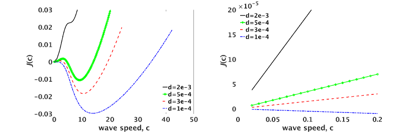
Figure 2: The computed values of ${\mathcal{J}(c)}$. Left: note the existence of multiple traveling pulse solutions for $d=3e-4$ and $d=5e-4$. Right: note that the curves do not cross the horizontal axis near $c=0$. For small values of $d$, the traveling pulse solution might be unique in the class -/+/-. For large values of $d$, there is no traveling pulse solution.

In Figure 2, note that ${\mathcal{J}(c)}$ crosses the horizontal axis twice when $d=5e-4$ and $d=3e-4$, but only once in case $d=1e-4$. Also, we see that for large enough values of $d$ there is no traveling pulse solution in the class ${-/+/-}$. In case of multiple roots of ${\mathcal{J}(c)}$, let $c_{1}=c_{1}(d)$ and $c_{0}=c_{0}(d)$ denote the smaller and larger of the wave speeds, respectively, such that ${\mathcal{J}(c)}=0$. Our computations suggest that there exists some critical value $d_{crit}$ such that

$$\lim_{d\to d_{crit}^{+}}c_{1}(d)=0.$$

Furthermore, for $d<d_{crit}$ the traveling wave solution might be unique in the class -/+/-. Stability of the traveling pulses is discussed below in Section 5.3.

In Table 2 we have provided the computed values of the ratio

$$\eta\equiv\frac{2dc_{0}^{2}}{(1-2\beta)^{2}}.$$

In accordance with (11), as the value of $d$ decreases we see the ratio $\eta$ becomes closer to the limiting value of $\eta=1$.

$d$	$c_{1}$	$c_{0}$	$\eta$
$5e-4$	$4.58$	$14.04$	$0.79$
$3e-4$	$3.14$	$19.18$	$0.88$
$1e-4$	—	$34.70$	$0.96$

Table 2: Computed values of the wave speeds $c_{0}$ and $c_{1}$ for traveling pulse solutions.

5.3 Testing of candidate traveling pulse profiles

Our computed traveling pulses are tested here via the method in Section 5.1. That is, the computed wave profiles, after scaling back from spatial variables $z$ to $x$, are used to initiate a parabolic solver and the computational window is moved at a rate of one grid length per time step. The grid length, $h$, and time step size, $\Delta t$, are related by $c\Delta t=h$ with $c$ the computed speeds in Table 2, so that the wave profile should move at the same rate as the computational window. A stable profile should then retain its shape and speed for a long time. The calculations were run for each case until either the profile was observed to break up or until the pulse propagated the distance of one computational domain length.

For the slower wave profiles with speed $c_{1}$, our tests showed that the profiles were not maintained by the parabolic solver, nor did they evolve into a new traveling pulse profile. Indeed, the profiles broke up completely after a relatively small time. An example is shown for $d=5e-4$ in Figure 1 (top). The slower traveling pulse solutions that exist for larger values of $d$ are unstable.

For the faster wave speeds denoted by $c_{0}$, we observed that the wave profiles remained stable. In Figure 3 the initial data is plotted together with the final data, upon completion of the parabolic solver run. The final data is shifted left in space by one domain length for a direct, visual comparison with the initial data. The profiles have traveled the length of their computational domain and retained their shape and speed very well in all cases.

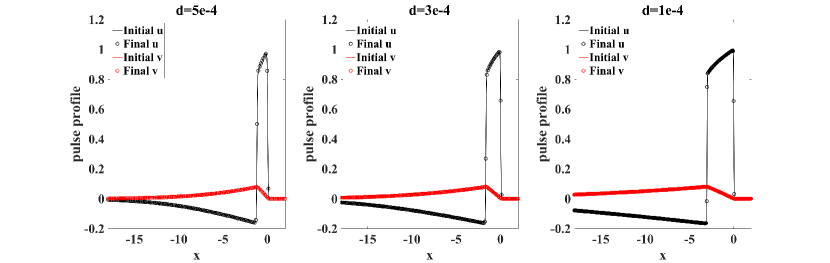
Figure 3: Computed pulse profiles, shifted back in space by one domain length for comparison with the initial profiles, for cases $d=5e-4$ (left), $d=3e-4$ (middle) and $d=1e-4$ (right). Circle markers are shown $200$ grid points apart for the final profiles. The initial and final profiles are visually identical, indicating stability.

6 Computation of pulses in two dimensions

In this section we demonstrate the calculation of traveling (dissipative) solitons in a multiple-dimensional domain. Partial curves ${\mathcal{J}(c)}$ are shown for four values of $d$, illustrating cases where there are multiple, one or no solutions found, including solitons and unstable pulses. A fundamental difference between the one- and two-dimensional cases relates to an occurrence of bifurcation in the latter case, wherein a soliton is observed to split into two co-evolving spots in the direction perpendicular to their motion.

We take $\Omega=(-\infty,\infty)\times(-L,L)$, with $L=1$ in all cases. As discussed in Section 4, we rescale the domain to $\Omega^{*}=(-\infty,\infty)\times(-cL,cL)$; the truncated, computational domain for Algorithm 1 is then chosen to be $[a,b]\times[-c,c]$. Recall that the domain is shifted during iterations of Algorithm 1, so we only specify the domain length $b-a$ below. Let $(x,y)$ and $(x^{*},y^{*})$ denote elements of $\Omega$ and $\Omega^{*}$, respectively.

Numerical methods to compute pulse profiles and for numerical integration are simple extensions of the methods described in Section 5.1 into two dimensions. That is, standard second-order, centered finite differences were used on a uniform rectangular grid to implement Algorithm 1. Numerical integration was implemented using midpoint approximations on each grid rectangle, also with centered, second-order rules to evaluate the terms of the integrands. The parabolic solver for stability tests is also analogous to that of Section 5.1, using centered finite differences in space and time stepping via Crank-Nicolson. Other relevant parameter values are given in Table 3. We apply asymptotic boundary conditions, as per Appendix A.

$\beta$	$\gamma$	$\theta$	$\alpha^{0}$	$\delta_{1}$	$\delta_{2}$	$\delta_{3}$
$1/4$	$1/16$	$1/2$	$10^{-5}-10^{-3}$	$10^{-6}$	$10^{-12}$	$10^{-3}-10^{-1}$

Table 3: Parameter values for the tests corresponding to Figure 4.

The functional values ${\mathcal{J}(c)}$ are shown for three values of $d$ in Figure 4. For these computations we fixed $b-a=280$, with $5600$ grid intervals from $x^{*}=a$ to $x^{*}=b$ and $80$ grid intervals from $y^{*}=-c$ to $y^{*}=c$. We observe that for $d=5e-4$ and $d=7e-4$ a single traveling soliton is found; that is, there is a single root of ${\mathcal{J}(c)}$ at $c=c_{0}$. We calculate $c_{0}\approx 13.74$ for $d=5e-4$ and $c_{0}\approx 10.54$ for $d=7e-4$. When $d=9e-4$, the root is lost and no solution is found.

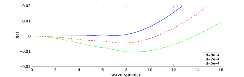
Figure 4: The computed values of ${\mathcal{J}(c)}$ in two dimensions, for three choices of $d$. For smaller values of $d$ we find one traveling pulse solution. For $d=9e-4$, ${\mathcal{J}(c)}$ remains above the horizontal axis and we observe no solution. A transitional behavior is observed for values of $c$ near $6$, due to the splitting of a soliton.

The computed solitons for both cases $d=5e-4$ and $d=7e-4$ were confirmed to be stable upon inserting these as initial conditions for a parabolic solver and allowing the spots to propagate for the length of one computational domain. Upon completion, we shift the solitons back to the left by the same distance, for a direct comparison with the initial profile. In Figure 5, we show that the initial and final profiles are visually identical.

Figure 5: Contour plots of $u$. Plot (a) shows the soliton profile, as computed using Algorithm 1 for $d=5e-4$, rescaled to variables $(x,y)$. The profile is then used to initiate a parabolic solver, then run until the soliton has propagated one domain length. Plot (b) shows the resulting profile, shifted back horizontally to compare with the initial profile. For $d=7e-4$, plot (c) shows the initial profile and (d) shows the final profile. The final profiles are visually identical to the initial profiles. These are stable; that is, they are traveling dissipative solitons.

A close inspection of Figure 4 reveals that ${\mathcal{J}(c)}$ appears to have a local maximum near $c=6$. This is related to a bifurcation that occurs. As we track only the minimum energy curve, there may be additional secondary bifurcations associated with other bifurcation branches, resulting in many close-by solutions. To illustrate this effect clearly, we consider the case of $d=8.8e-4$, for which the values of ${\mathcal{J}(c)}$ are plotted in Figure 6. The curve ${\mathcal{J}(c)}$ versus $c$ has two smooth branches, separated near $c\approx 6.1$. For larger $c$, the minimizer profile has one contiguous positive region. That is, there is a single soliton. As $c$ decreases, a separation into two parallel solitons serves to reduce the energy. This qualitative state persists for the minimizer profile as $c$ decreases toward zero. As a result, we found four roots of ${\mathcal{J}(c)}$ corresponding to two solitons and two unstable traveling pulses.

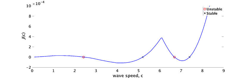
Figure 6: The computed values of ${\mathcal{J}(c)}$ for $d=8.8e-4$. A bifurcation occurs near $c\approx 6.1$. As a result, four solutions are found; two solitons and two are unstable pulses.

We denote the four wave speeds for the traveling pulses by $c_{0}\approx 7.4067$, $c_{1}\approx 6.6864$, $c_{2}\approx 5.1752$ and $c_{3}\approx 2.4181$. The unstable pulses correspond to $c_{1}$ and $c_{3}$. In Figure 7 we show the unstable computed profiles $u$, rescaled to variables $(x,y)$, as computed by Algorithm 1.

The stable solitons correspond to $c_{0}$ and $c_{2}$. In Figure 8 we show these, rescaled to variables $(x,y)$, as computed by Algorithm 1 and also after running the parabolic solver to demonstrate stability. For visualization purposes, we do not show the entire domain. We note that the computational grid used for these computations with $c>6.1$, corresponding to the single-soliton solution, was the same as for other computations in this section. However, for $c<6.1$ the computational domain was shortened so that $b-a=50$, with 4000 intervals between $x^{*}=a$ and $x^{*}=b$ and $160$ computational intervals between $y^{*}=-c$ and $y^{*}=c$. This finer computational grid was needed to approximate the two-soliton solution. In Figure 8 we note that the computed solitons retain their shapes well, but they do not travel with precisely the computed wave speeds $c_{0}$ and $c_{2}$. We believe this is simply due to numerical error in computing the functional value $J_{c}(u)$, which could be reduced using a finer computational grid or more accurate finite difference method. For $d=8.8e-4$, the values of ${\mathcal{J}(c)}$ remain very small over a wide range of $c$ values. As a result, it is more difficult to compute the location of the roots of ${\mathcal{J}(c)}$ as compared to other examples in this paper.

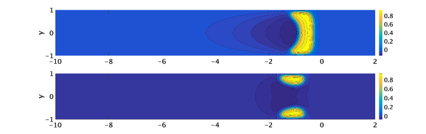
Figure 7: Contour plots of the unstable traveling pulse profiles $u$ for $d=8.8e-4$. Top: the profile with wave speed $c_{1}$. Bottom: the double-pulse with wave speed $c_{3}$.

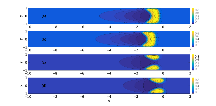
Figure 8: Contour plots of the traveling solitons for $d=8.8e-4$. Plot (a) shows the profile $u$ as computed using Algorithm 1, rescaled to variables $(x,y)$. The profile is then used to initiate a parabolic solver, run until the soliton propagates one domain length. Plot (b) shows the resulting profile, shifted back horizontally to compare with the initial profile. For the two-soliton solutions, plot (c) shows the initial profile and (d) shows the final profile, shifted back horizontally.

7 Summary and future work

We have provided an iterative method to calculate traveling solitons and unstable traveling pulse solutions for the FitzHugh-Nagumo equations. It is a steepest descent method based on the minimization of a functional within a certain admissible set. The infimum of the functional over the admissible set, denoted by ${\mathcal{J}(c)}$, depends on a parameter $c$ that represents wave speed. Traveling pulses are identified as roots of the functional; ${\mathcal{J}(c)}=0$. We have demonstrated that the method is robust. For example, some tests revealed that initial guesses employed for our method would not suffice as initial conditions in a parabolic solver to try to compute a soliton. The computations also support the asymptotic relationship (11) that applies to the solitons (observed as the fastest pulses), given a set of physical parameters. This provides mutual validation. We computed both stable and unstable traveling pulses for moderate values of the parameter $d$, no traveling pulses for large values of $d$ and a unique, stable traveling pulse for small $d$. Solitons were tested using a parabolic solver and observed to be stable.

We also observe that as $d$ becomes small, the fastest wave speed for the soliton becomes large, the pulse width (measured in an appropriate sense) becomes wide, and the tail decay rate becomes slow. Due to the steep wave front but otherwise smooth and slowly-decaying tail, our use of uniform grids with finite difference methods is not optimal. This could be addressed through the use of adaptive methods. For example, the class of $hp$-adaptive finite element methods have previously enjoyed success for problems with a wide range of scales (see e.g. Devloo et al. (1988)).

In two dimensions of space, we observed a bifurcation that qualitatively separates single and double traveling soliton solutions. The splitting of the solitons from one to two spots serves to lower the functional energy ${\mathcal{J}(c)}$ as $c$ decreases (below around $c\approx 6$ in our examples). For a narrow range of parameter values, this enables ${\mathcal{J}(c)}$ to drop below zero multiple times as $c$ changes, resulting in four traveling pulse solutions for a single set of parameters, with their speeds distinct. Two solutions are unstable. The two-soliton solutions have smaller wave speeds than the single-soliton solutions.

In some on-going work Choi et al. , we will demonstrate how to use our algorithm to find traveling fronts as well in 2D. In fact, for the same physical parameters, fronts and pulses can co-exist. Our steepest descent method can find many traveling waves independently for systems with a variational structure, but it could also serve as a robust tool to augment the use of continuation methods, which may have difficulty in multiple dimensions sometimes (see Section 1). Conceivably, one might also use the global property to create an ad-hoc continuation-steepest descent method that can take larger steps along a bifurcation curve, saving total computational expense for detailed explorations of parameter space.

Appendix A  Algorithm 1 with asymptotic boundary conditions

The traveling pulses decay to zero as $|x|\to\infty$ for both one- or two-dimensional domains. Instead of imposing the zero Dirichlet boundary condition on the bounded computational domain in Algorithm 1, we derive asymptotic boundary conditions that provide better information on solution behaviors as $|x|\to\infty$ than just knowing that they go to zero. If the governing equation is linear, eliminating the blow-up mode will yield the asymptotic information. Similar conclusions can be drawn by linearizing the nonlinear equations about the zero equilibrium point. Such an idea has been given in, for example, Lentini and Keller (1980).

Specifically, we derive asymptotic boundary conditions to solve for $v={\mathcal{L}_{c}}w$ and $w^{*}={\mathcal{Q}}(w)$ in Steps 1 and 3 of Algorithm 1. In practice, we have found that the minimum computational domain lengths are restricted by these calculations, whereas the integrations in Steps 2 and 6 exhibit faster convergence. This is because as $x\to\infty$, the pulse profiles vanish very quickly, while when $x\to-\infty$ the term $e^{x}$ in the integrands forces the fast convergence of the integrals even though the profiles do not vanish as quickly in this direction. For these reasons, we neglect further discussion of errors in integrated quantities due to the truncation of the domain.

A.1 Computing ${{\mathcal{L}_{c}}w}$ and $w^{*}$ with a given $w$ in one dimension

Suppose a function $w$ is defined on the real line $(-\infty,\infty)$; however it is known only on the interval $[a,b]$. First, we will construct asymptotic boundary conditions for Step 1 in Algorithm 1. As $w$ serves as a guess of the minimizer $u$ which decays to zero at infinity, we assume $w$ and $w^{\prime}$ are $o(1)$ outside the interval $[a,b]$. Let $v={\mathcal{L}_{c}}w$. Then $v^{\prime\prime}+v^{\prime}-\frac{\gamma}{c^{2}}v=-\frac{w}{c^{2}}$ on $(-\infty,\infty)$, which is equivalent to the system

$$\left(\begin{array}[]{c}v\\ z\end{array}\right)^{\prime}=B\left(\begin{array}[]{c}v\\ z\end{array}\right)-\left(\begin{array}[]{c}0\\ \frac{w}{c^{2}}\end{array}\right)$$ (33)

where $B=\left(\begin{array}[]{cc}0&1\\ \frac{\gamma}{c^{2}}&-1\end{array}\right)$. The eigenvalues of $B$ are given by

$$\left\{\nu_{1}\,,\,\nu_{2}\right\}=\left\{\frac{1}{2}\left(-1-\sqrt{1+\frac{4\gamma}{c^{2}}}\right)\,,\,\frac{1}{2}\left(-1+\sqrt{1+\frac{4\gamma}{c^{2}}}\right)\right\},$$ (34)

with $\nu_{1}<-1<0<\nu_{2}$. Correspondingly, ${\bf L}_{1}=\left(\begin{array}[]{c}-\nu_{2}\\ 1\end{array}\right)$ and ${\bf L}_{2}=\left(\begin{array}[]{c}-\nu_{1}\\ 1\end{array}\right)$ are the left eigenvectors of $B$ for $\nu_{1}$ and $\nu_{2}$, respectively. By taking the scalar product of ${\bf L}_{1}$ with (33), we obtain

$$\Phi_{1}^{\prime}=\nu_{1}\Phi_{1}-\frac{w}{c^{2}}$$ (35)

where $\Phi_{1}\equiv{\bf L}_{1}\cdot\left(\begin{array}[]{c}v\\ z\end{array}\right)=-\nu_{2}v+z$. This first order equation can be integrated to give

$$\Phi_{1}(x)=-\int_{-\infty}^{x}e^{\nu_{1}(x-t)}\frac{w(t)}{c^{2}}dt;$$

the arbitrary constant associated with the complementary solution has to be set to zero for $\Phi_{1}$ to stay bounded as $x\to-\infty$. It follows that

$$\nu_{1}\Phi_{1}(a)-\frac{w(a)}{c^{2}} = \frac{\nu_{1}}{c^{2}}\int_{-\infty}^{a}e^{\nu_{1}(a-t)}(w(a)-w(t))\,dt$$

$$= -\frac{1}{c^{2}}\int_{-\infty}^{a}e^{\nu_{1}(a-t)}w^{\prime}(t)\,dt.$$

Hence

$$\left|\nu_{1}\Phi_{1}(a)-\frac{w(a)}{c^{2}}\right| \leq \frac{|o(1)|}{c^{2}}\int_{-\infty}^{a}e^{\nu_{1}(a-t)}\,dt.$$

$$= \frac{|o(1)|}{|\nu_{1}|\,c^{2}}\;.$$

It is therefore natural to impose the boundary condition $\nu_{1}\Phi_{1}=\frac{w}{c^{2}}$ at $x=a$; which amounts to

$$v^{\prime}-\nu_{2}v=\frac{w}{\nu_{1}c^{2}}\quad\mbox{at}\;\;x=a.$$ (36)

This is like setting the right hand side of (35) to zero at $x=a$. A similar analysis for large positive $x$ using $\Phi_{2}={\bf L}_{2}\cdot\left(\begin{array}[]{c}v\\ z\end{array}\right)$ leads to

$$v^{\prime}-\nu_{1}v=\frac{w}{\nu_{2}c^{2}}\quad\mbox{at}\;\;x=b.$$ (37)

(36) and (37) are the asymptotic boundary conditions used when solving for $v={\mathcal{L}_{c}}w$.

Remark 4

If $w$ goes to different constants as $x\to\pm\infty$ but with $w^{\prime}=o(1)$ beyond $[a,b]$, the above argument can be modified to derive some different asymptotic boundary conditions. This observation will have implications in case one studies a traveling front problem numerically.

We will now compute $w^{*}$ from (21) in Step 3 of Algorithm 1 using asymptotic boundary conditions. Let $\hat{w}=dc^{2}w-{\mathcal{L}_{c}}w+f(w)$ denote the known right hand side of (21). Compare this problem with the equation on $v$ in Section A.1. By substituting $\gamma/c^{2}$ by $1$ and $w/c^{2}$ by $\hat{w}$, the new eigenvalues now are $\nu_{1}^{*}=-\frac{1}{2}(1+\sqrt{5})$ and $\nu_{2}^{*}=\frac{1}{2}(\sqrt{5}-1)$, and the asymptotic boundary conditions are given by

$${w^{*}}{\,{}^{\prime}}-\nu_{2}^{*}w^{*} =\frac{\hat{w}}{\nu_{1}^{*}} \mbox{at}\;\;x=a,$$ (38)

$${w^{*}}{\,{}^{\prime}}-\nu_{1}^{*}w^{*} =\frac{\hat{w}}{\nu_{2}^{*}} \mbox{at}\;\;x=b.$$ (39)

A.2 Computing ${{\mathcal{L}_{c}}w}$ and $w^{*}$ with a given $w$ in two dimensions

We take $w=w(x,y)$ on the infinite strip $(-\infty,\infty)\times[-L,L]$ and derive asymptotic boundary conditions to apply on the truncated domain $\Omega=[a,b]\times[-L,L]$, first for $v={\mathcal{L}_{c}}w$. At $y=-L$ and $y=L$ the boundary values are $w=v=0$, for all $x\in\mathbb{R}$. Fourier expansions for $v={\mathcal{L}_{c}}w$ and $w$ are

$$w(x,y) =\sum_{j=1}^{\infty}\hat{w}_{j}(x)\sin\left(\frac{j\pi(y+L)}{2L}\right),$$ (40)

$$v(x,y) =\sum_{j=1}^{\infty}\hat{v}_{j}(x)\sin\left(\frac{j\pi(y+L)}{2L}\right).$$

Insert the relations (40) into the equation $\Delta v+v_{x}-\frac{\gamma}{c^{2}}v=-\frac{1}{c^{2}}w$:

$$\sum_{j=1}^{\infty}\left(\hat{v}_{j}^{\prime\prime}(x)+\hat{v}_{j}^{\prime}(x)-\left(\frac{j^{2}\pi^{2}}{4L^{2}}+\frac{\gamma}{c^{2}}\right)\hat{v}_{j}(x)\right)\sin\left(\frac{j\pi(y+L)}{2L}\right)=\\ \sum_{j=1}^{\infty}-\frac{1}{c^{2}}\hat{w}_{j}(x)\sin\left(\frac{j\pi(y+L)}{2L}\right).$$

Then the Fourier coeffcients satisfy

$$\hat{v}_{j}^{\prime\prime}(x)+\hat{v}_{j}^{\prime}(x)-\left(\frac{j^{2}\pi^{2}}{4L^{2}}+\frac{\gamma}{c^{2}}\right)\hat{v}_{j}(x)=-\frac{1}{c^{2}}\hat{w}_{j}(x).$$ (41)

In case $x<0$ with $|x|\gg 1$, we assume it holds that $|\hat{w}_{j}(x)|\ll|\hat{w}_{1}(x)|$ and $|\hat{v}_{j}(x)|\ll|\hat{v}_{1}(x)|$ for all $j>1$, thus

$$w(x,y) \approx\hat{w}_{1}(x)\sin\left(\frac{\pi(y+L)}{2L}\right),$$ (42)

$$v(x,y) \approx\hat{v}_{1}(x)\sin\left(\frac{\pi(y+L)}{2L}\right).$$

Then $\hat{w}_{1}(x)$ and $\hat{v}_{1}(x)$ have the same behavior in $x$ as $w$ and $v$, respectively, as $x\to-\infty$. Furthermore, these Fourier coefficients satisfy (41). By analogy with the derivation in Section A.1, if $a<0$ with $|a|\gg 1$ then we apply the boundary condition

$$\hat{v}_{1}^{\prime}-\nu_{2}\hat{v}_{1}=\frac{\hat{w}_{1}}{\nu_{1}c^{2}}\quad\mbox{at}\;\;x=a$$ (43)

with the eigenvalues

$$\nu_{1} =\frac{1}{2}\left(-1-\sqrt{1+\frac{\pi^{2}}{L^{2}}+\frac{4\gamma}{c^{2}}}\right)$$ (44)

$$\mbox{and}\;\;\nu_{2} =\frac{1}{2}\left(-1+\sqrt{1+\frac{\pi^{2}}{L^{2}}+\frac{4\gamma}{c^{2}}}\right).$$

We combine (42) and (43) to derive the approximate boundary condition

$$\frac{\partial v}{\partial x}-\nu_{2}v=\frac{w}{\nu_{1}c^{2}}\quad\mbox{at}\;\;x=a,\quad\mbox{for}\;\;-L<y<L.$$ (45)

It is equivalent to applying (36) at $x=a$ for each fixed value of $y$, with the adjustment (44) for the eigenvalues (34). The corresponding boundary condition on the right is

$$\frac{\partial v}{\partial x}-\nu_{1}v=\frac{w}{\nu_{2}c^{2}}\quad\mbox{at}\;\;x=b,\quad\mbox{for}\;\;-L<y<L,$$ (46)

by analogy with (37) and the derivation of (45). Here, we assume $b\gg 1$. Taken together with $v(x,-L)=v(x,L)=0$ for all $x\in\mathbb{R}$, (45)-(46) are the boundary conditions used to compute $v={\mathcal{L}_{c}}w$ on the truncated domain. Note that the asymptotic conditions (45)-(46) are compatible with the homogeneous Dirichlet boundary conditions for $v$ and $w$ at $y=\pm L$.

Asymptotic boundary conditions for $w^{*}$ in Step 3 of Algorithm 1 may be derived quickly by first comparing (21) to the equation (27) for $v={\mathcal{L}_{c}}w$. Let $\tilde{w}=dc^{2}w-{\mathcal{L}_{c}}w+f(w)$ denote the known right hand side of (21). By substituting $\gamma/c^{2}$ with $1$ and $w/c^{2}$ with $\tilde{w}$, the new eigenvalues now are

$$\left\{\nu^{*}_{1}\,,\,\nu^{*}_{2}\right\}=\left\{\frac{1}{2}\left(-1-\sqrt{5+\frac{\pi^{2}}{L^{2}}}\right)\,,\,\frac{1}{2}\left(-1+\sqrt{5+\frac{\pi^{2}}{L^{2}}}\right)\right\},$$ (47)

and the asymptotic boundary conditions are given by

$$\frac{\partial w^{*}}{\partial x}-\nu_{2}^{*}w^{*} =\frac{1}{\nu_{1}^{*}}\tilde{w} \mbox{at}\;\;x=a,\;\;-L<y<L,$$ (48)

$$\frac{\partial w^{*}}{\partial x}-\nu_{1}^{*}w^{*} =\frac{1}{\nu_{2}^{*}}\tilde{w} \mbox{at}\;\;x=b,\;\;-L<y<L.$$ (49)

References

- Akhmediev and Ankiewicz (2005) Akhmediev, N. and Ankiewicz, A. (2005). Dissipative solitons, volume 661 of Lecture Notes in Phys. Springer, Berlin.
- Chen et al. (2016) Chen, C.-N., Chen, C.-C., and Huang, C.-C. (2016). Traveling waves for the FitzHugh-Nagumo system on an infinite channel. J. Differential Equations, 261(6):3010–3041.
- Chen and Choi (2012) Chen, C.-N. and Choi, Y. S. (2012). Standing pulse solutions to FitzHugh-Nagumo equations. Arch. Ration. Mech. Anal., 206(3):741–777.
- Chen and Choi (2015) Chen, C.-N. and Choi, Y. S. (2015). Traveling pulse solutions to FitzHugh-Nagumo equations. Calc. Var. Partial Differential Equations, 54(1):1–45.
- Chen and Choi (2018) Chen, C.-N. and Choi, Y.-S. (2018). Front propagation in both directions and coexistence of traveling fronts and pulses, submitted.
- (6) Chen, C.-N., Choi, Y.-S., and Fusco, N. The -limit of traveling waves in the FitzHugh-Nagumo system, submitted.
- Chen et al. (2018a) Chen, C.-N., Choi, Y.-S., Hu, Y., and Ren, X. (2018a). Higher dimensional bubble profiles in a sharp interface limit of the FitzHugh-Nagumo system. SIAM J. Math. Anal., 50(5):5072–5095.
- Chen et al. (2018b) Chen, C.-N., Choi, Y.-S., and Ren, X. (2018b). Bubbles and droplets in a singular limit of the FitzHugh-Nagumo system. Interfaces Free Bound., 20(2):165–210.
- (9) Choi, Y. S., Connors, J., and Duraihem, F. Co-existence of a traveling pulse with multiple moving fronts: a numerical investigation. In preparation.
- Choi and McKenna (1993) Choi, Y. S. and McKenna, P. J. (1993). A mountain pass method for the numerical solution of semilinear elliptic problems. Nonlinear Anal., 20(4):417–437.
- Dancer et al. (2007) Dancer, E. N., Ren, X., and Yan, S. (2007). On multiple radial solutions of a singularly perturbed nonlinear elliptic system. SIAM J. Math. Anal., 38(6):2005–2041.
- Devloo et al. (1988) Devloo, P., Oden, J. T., and Pattani, P. (1988). An h-p adaptive finite element method for the numerical simulation of compressible flow. Computer Methods in Applied Mechanics and Engineering, 70(2):203 – 235.
- Ei et al. (2006) Ei, S.-I., Mimura, M., and Nagayama, M. (2006). Interacting spots in reaction diffusion systems. Discrete Contin. Dyn. Syst., 14(1):31–62.
- Kawaguchi and Mimura (2008) Kawaguchi, S. and Mimura, M. (2008). Synergistic effect of two inhibitors on one activator in a reaction-diffusion system. Phys. Rev. E (3), 77(4):046201, 17.
- Lentini and Keller (1980) Lentini, M. and Keller, H. B. (1980). Boundary value problems on semi-infinite intervals and their numerical solution. SIAM J. Numer. Anal., 17(4):577–604.
- Liehr (2013) Liehr, A. W. (2013). Dissipative solitons in reaction diffusion systems. Springer Series in Synergetics. Springer, Heidelberg. Mechanisms, dynamics, interaction.
- Muratov (2004) Muratov, C. B. (2004). A global variational structure and propagation of disturbances in reaction-diffusion systems of gradient type. Discrete Contin. Dyn. Syst. Ser. B, 4(4):867–892.
- Nishiura (2002) Nishiura, Y. (2002). Far-from-equilibrium dynamics, volume 209 of Translations of Mathematical Monographs. American Mathematical Society, Providence, RI. Translated from the 1999 Japanese original by Kunimochi Sakamoto, Iwanami Series in Modern Mathematics.
- Nishiura et al. (2007) Nishiura, Y., Teramoto, T., Yuan, X., and Ueda, K.-I. (2007). Dynamics of traveling pulses in heterogeneous media. Chaos, 17(3):037104, 21.
- Purwins et al. (2005) Purwins, H.-G., Bödeker, H. U., and Liehr, A. W. (2005). Dissipative solitons in reaction-diffusion systems. In Dissipative solitons, volume 661 of Lecture Notes in Phys., pages 267–308. Springer, Berlin.
- Ren and Wei (2003) Ren, X. and Wei, J. (2003). On energy minimizers of the diblock copolymer problem. Interfaces Free Bound., 5(2):193–238.
- Stoer and Bulirsch (2010) Stoer, J. and Bulirsch, R. (2010). Introduction to Numerical Analysis. Springer-Verlag, 3 edition.
- Turing (1952) Turing, A. M. (1952). The chemical basis of morphogenesis. Philos. Trans. Roy. Soc. London Ser. B, 237(641):37–72.
- van Heijster et al. (2010) van Heijster, P., Doelman, A., Kaper, T. J., and Promislow, K. (2010). Front interactions in a three-component system. SIAM J. Appl. Dyn. Syst., 9(2):292–332.
- van Heijster and Sandstede (2014) van Heijster, P. and Sandstede, B. (2014). Bifurcations to travelling planar spots in a three-component FitzHugh-Nagumo system. Phys. D, 275:19–34.
- VonNeumann and Richtmyer (1950) VonNeumann, J. and Richtmyer, R. D. (1950). A method for the numerical calculation of hydrodynamic shocks. Journal of Applied Physics, 21(3):232–237.