HetNets Coverage Modeling and Analysis Over Fox’s $\mathcal{H}$-Fading Channels

Abstract

This paper embodies the Fox’s ${\mathcal{H}}$-transform theory into a unifying modeling and analysis of HetNets. The proposed framework has the potential, due to the Fox’s ${\mathcal{H}}$-functions versatility, of significantly simplifying the cumbersome analysis and representation of cellular coverage, while subsuming those previously derived for all known simple and composite fading models. The paper reveals important insights into the practice of densification in conjunction with signal-to-noise plus interference (SINR) thresholds and path-loss models.

I Introduction

Chiefly urged by the occurring mobile data deluge, a radical design make-over of cellular systems advocating heterogenous cellular networks (HetNets) is crucial and thus an active research trend [1]-​​[7]. The random space pattern of HetNets has been extensively reproduced and analyzed trough stochastic geometry over different fading channels such as Rayleigh [2], Nakagami-$m$ [6], Weibull [5] and $\alpha$-$\mu$ [4].

Besides subsuming most of these fading models, the Fox’s $\mathcal{H}$-distribution is currently being touted for its high flexibility to adapt different fading behaviors pertaining to emerging new wireless applications, e.g., device-to-device (D2D) and intervehicular communications, wireless body area networks, and millimeterwave (mmWave) communications [8]. Despite several studies on its applicability in evaluating various wireless communication (​[9] and references therein), the Fox’s $\mathcal{H}$-distribution has thus far not found its way into stochastic geometry-based cellular communications as a possible fading distribution. Yet, resorting to the most comprehensive treatments of the subject [2]-​​[10], a general analytic solution for Fox’s $\mathcal{H}$ fading seems unlikely, if not impossible. Indeed, besides being simple special cases, these treatments rely on approximating the fading distribution (e.g., integer fading parameter-based power series [6], [7], and Laguerre polynomial series in [10]) which hamper their generality and exactness. Moreover, these treatments usually entail computationally expensive Laplace generation functional evaluation lending the solution approach itself complicated and more importantly non applicable to the generalized Fox’s $\mathcal{H}$ fading.

To the best of the authors’ knowledge, no work has ever been found to analyze the coverage of HetNets over the general Fox’s $\mathcal{H}$ fading channels. The main contributions of this letter are as follows:

• Novel exact and closed-form expressions are derived for the coverage of HetNets over Fox’s $\mathcal{H}$-fading under both range expansion as well as max-SIR cell association (CA) rules. Our analysis procedure and coverage formulations are given in unified and tractable mathematical fashion thereby serving as a useful tool to validate and compare the special cases of Fox’s $\mathcal{H}$-fading channels.

• Some useful insights regarding the practice of densification of HetNets in conjunction with path-loss model are also provided through the asymptotic coverage analysis.

• The derived results enable to evaluate the impacts of physical channel and network dynamics such as fading parameters, density of BSs, SINR thresholds, and path-loss model on coverage performance.

II Channel and Network Models

II-A The Fox’s $\mathcal{H}$ Channel Model

Consider a wireless communication link over a fading channel where the power gain is distributed according to the Fox’s $\mathcal{H}$ $\{{\cal O},{\mathcal{P}}\}$ distribution with order sequence ${\mathcal{O}}=(m,n,p,q)$, parameter sequence ${\mathcal{P}}=(\kappa,c,a,b,A,B)$, and probability density function (PDF)

$$f_{H}(x)={\mathcal{\kappa}}{\mathcal{H}}_{p,q}^{m,n}\left[cx\left|\begin{array}[]{ccc}(a_{i},A_{j})_{p}\\ (b_{i},B_{j})_{q}\end{array}\right.\right],\quad x\geq 0,$$ (1)

where $c$ and $\kappa$ are constants, and $(x_{j},y_{j})_{l}$ is a shorthand notation for $(x_{1},y_{1}),...,(x_{l},y_{l})$. Hereafter, for notational simplicity, we denote the right-hand side of (1) by ${\mathcal{H}}_{p,q}^{m,n}(x;{\cal P})$.

II-B Special cases

A Fox’s H-function PDF considers homogeneous radio propagation conditions and captures composite effects of multipath fading and shadowing, subsuming large variety of extremely important or generalized fading distributions used in wireless communications as $\alpha$-$\mu$, $N$-Nakagami-$m$, (generalized) ${\cal K}$-fading, and Weibull/gamma fading , the Fisher-Snedecor F-S $\cal F$, and EGK, as shown in Table. I (​[9], [11] and references therein). Furthermore, the Fox’s H-function distribution provides enough flexibility to account for disparate signal propagation mechanisms and well-fitted to measurement data collected in diverse propagation environments having different parameters.

TABLE I: Special cases of Fox’s H-function distribution

$$\begin{array}[]{cc}\\ \!\!\!f_{H}(x)\sim\mathcal{H}\{{\cal O},{\mathcal{P}}\}\\ \hline\cr\begin{array}[]{c}\alpha-\mu\\ \end{array}&\\ \begin{array}[]{c}{\mathcal{O}}_{\alpha-\mu}=(1,0,0,1)\\ \!\!\!\!\!\!{\mathcal{P}}_{\alpha-\mu}=\left(\frac{\Gamma(\mu+\frac{1}{\alpha})}{\Gamma(\mu)^{2}},\kappa\Gamma(\mu),-,\mu-\frac{1}{\alpha},-,\frac{1}{\alpha}\right)\end{array}\\ \hline\cr\\ \textbf{F-S }{\cal F}&\\ \begin{array}[]{c}{\mathcal{O}}_{\textbf{F-S }{\cal F}}=(1,1,1,1)\\ \!\!\!\!\!\!{\mathcal{P}}_{\textbf{F-S }{\cal F}}=\left(\frac{c}{\Gamma(m)\Gamma(m_{s})},\frac{m}{m_{s}},-m_{s},m-1,1,1\right)\end{array}\\ \hline\cr\\ \textbf{EGK}&\\ \begin{array}[]{c}{\mathcal{O}}_{\textbf{EGK}}=(2,0,0,2)\\ \!\!\!\!\!\!{\mathcal{P}}_{\textbf{EGK}}=\left(\frac{\beta\beta_{s}}{\Gamma(m)\Gamma(\kappa)},\beta\beta_{s},-,(m-\frac{1}{\zeta},\kappa_{s}-\frac{1}{\zeta}),-,(\frac{1}{\zeta},\frac{1}{\zeta})\right)\\ \text{where}~{}\beta=\frac{\Gamma(m+\frac{1}{\zeta})}{\Gamma(m)}~{}\text{and}~{}\beta_{s}=\frac{\Gamma(\kappa_{s}+\frac{1}{\zeta})}{\Gamma(m)}\end{array}\\ \hline\cr\end{array}$$

II-C Network Model

Consider the downlink of a ${\cal M}$-tier HetNet. Each tier is specified by the tuple $(\lambda_{i},P_{i},\beta_{i},\{{\cal O}_{i},{\mathcal{P}}_{i}\}),i\in\{1,\ldots,{\cal M}\}$, indicating the BS spatial density, transmission power, target SINR threshold, and the order and parameters sequences of the $\mathcal{H}$-fading, respectively. The BSs in the $i$-th tier are spatially distributed as a homogenous Poisson point process (PPP) $\Phi_{i}\in\mathbb{R}^{2}$ with density $\lambda_{i}$. Let $H_{x_{i}}$ be the channel power gain between BS $x_{i}\in\Phi_{i}$to be distributed according to the Fox’s $\mathcal{H}$-distribution $\{{\cal O}_{i},{\mathcal{P}}_{i}\}$. Furthermore, we denote $L(\|x\|)$ the path-loss function and

$${\cal I}=\sum_{i\in{\cal M}}\sum_{x_{i}\in\Phi_{i}/x_{k}}P_{i}L(\|x_{i}\|)H_{x_{i}},$$ (2)

the aggregate interference at a typical receiver, assuming that its serving BS belongs to the $k$-th tier. The SINR at the typical receiver can then be formulated as

$$\text{SINR}^{m}_{x_{k}}=\frac{P_{k}L(\|x_{k}\|)H_{x_{k}}}{{\cal I}+\sigma^{2}_{k}},$$ (3)

where $\sigma^{2}_{k}$ is the thermal noise power associated with the $k$-th tier, and the parameter $m\in\{{\cal U},{\cal B}\}$ where i) $m={\cal U}$ stands for the unbounded path-loss scenario, i.e., $L(\|x\|)=\|x\|^{-\alpha}$ where $\alpha$ is the path-loss exponent and ii) $m={\cal B}$ uses the bounded path-loss model, i.e., $L(\|x\|)=(1+\|x\|)^{-\alpha}$.

III Fox’s $\mathcal{H}$ Modeling of Coverage

III-A RSS Cell Association

Let the typical user be associated with the BS that provides the maximum radio signal strength (RSS). This implies that the typical user is then in coverage if the set ${\cal A}^{m}=\left\{\exists i\in{\cal M}:i=\arg\max_{j\in{\cal M},x\in\Phi_{j}}P_{j}L(\|x_{j}\|);\text{SINR}^{m}_{x_{i}}\geq\beta_{i}\right\}$ is not empty. Let us denote $r_{k}=\|x_{k}\|$ and define the coverage probability by ${\cal C}^{m}=P\{{\cal A}^{m}\neq\varnothing\}$. ${\cal C}^{m}\triangleq\sum^{{\cal M}}_{k=1}{\cal\theta}_{k}\mathcal{E}_{r_{k}}\{{\cal C}^{m}(r_{k})\}$ where ${\cal\theta}_{k}=\frac{\lambda_{k}}{\sum_{j\in{\cal M}}\lambda_{j}\widetilde{P}_{j}^{\delta}}$.

Proposition 1: The average coverage probability Fox’s $\mathcal{H}$-fading with an unbounded path loss model is given by

$$\!\!\!\!\!\!\!{\cal C}^{\cal U}\!\!\! = \!\!\!\pi\delta\sum^{{\cal M}}_{k=1}\lambda_{k}\left(\frac{P_{k}}{\sigma_{k}^{2}}\right)^{\delta}\int_{0}^{\infty}\frac{1}{\xi^{2+\delta}}{\mathcal{H}}_{q,p+1}^{n,m}\left(\xi,{\cal P}^{k}_{\cal U}\right)$$ (4)

$$\!\!\!\!\!\!\!\!\!\!\!\!\!\!\!\!\!\!\!\!\!\!\!\!{\mathcal{H}}_{1,1}^{1,1}\!\!\left(\!\!\frac{\left(\frac{P_{k}}{\sigma^{2}_{k}}\right)^{\delta}}{\xi^{\delta}}\!\!\sum_{j\in{\cal M}}\!\!\!\pi\lambda_{j}\widetilde{P}^{\delta}_{j}\!\left(1\!+\!\delta\xi{\mathcal{H}}_{q+2,p+3}^{n+1,m+2}\!\!\left(\xi,{\cal P}^{{\cal I}}_{\cal U}\right)\!\right)\!,\!{\cal P}_{\delta}\!\!\right)\!d\xi,$$

where ${\cal P}^{k}_{\cal U}=\!\!\left(\kappa{\cal\beta}_{k},\frac{1}{c{\cal\beta}_{k}},1\!-\!b,(1\!-\!a,1),\mathcal{B},(A,1)\right),$ and ${\cal P}^{{\cal I}}_{\cal U}=\bigg{(}\frac{\kappa}{c^{2}},\frac{1}{c},(1\!-\!b\!-\!2B,0,\delta),(0,1\!-\!a\!-\!2A,-1,\delta\!-\!1),$ $(\mathcal{B},1,1),(1,A,1,1)\bigg{)}$, and ${\cal P}_{\delta}=\left(1,1,1-\delta,0,\delta,1\right)$.

Proof: See Appendix A.
The new fundamental SINR distribution disclosed in Proposition 1 provides an exact and numerically inexpensive unifying tool for coverage analysis in a variety of extremely important fading distributions (see [11, Table I]). In some particular cases, the obtained formulas reduces to previously well-known major results in the literature [2],​[3],​ [6].

Corollary 1 (HetNets densification in Fox’s $\mathcal{H}$-fading with unbounded path-loss model): The average coverage of ultra-dense networks with RSS under unbounded path-loss scales as

$$\lim_{\lambda\rightarrow\infty}{\cal C}^{\cal U}=$$ (5)

$$\!\!\!\!\!\!\!\!\!\!\!\!\!\!\!\!\!\!\!\!\!\!\!\!\!\!\!\!\!\!\!\sum^{{\cal M}}_{k=1}\!\int_{0}^{\infty}\frac{{\mathcal{H}}_{q,p+1}^{n,m}\left(\xi,{\cal P}^{k}_{\cal U}\right)d\xi}{\xi^{2}\sum_{j\in{\cal M}}\!\widetilde{P}^{\delta}_{j}\!\left(1\!+\!\delta\xi{\mathcal{H}}_{q+2,p+3}^{n+1,m+2}\!\!\left(\xi,{\cal P}^{{\cal I}}_{\cal U}\right)\right)}.$$

Proof: Recall that the asymptotic expansion of the Fox’s $\mathcal{H}$-function near $x=\infty$ given by [13, Eq. (1.5.9)]

$${\mathcal{H}}_{p,q}^{m,n}(x;{\cal P})\underset{x\rightarrow\infty}{\approx}\kappa\eta x^{d},$$ (6)

where $d=\max\left(\frac{a_{i}-1}{A_{i}}\right),i=1,\ldots,n$ and $\eta$ is calculated as in [13, Eq. (1.5.10)]. Applying (6) to (4) when $\lambda_{k}=\lambda\rightarrow\infty,k=1,\ldots,{\cal M}$, yields the result after recognizing that $d=-1$ and $\eta=\frac{1}{\delta}$.

Corollary 1 shows how the singularity in the unbounded model can affect the accountability of the conducted analysis, since the coverage intensity-invariance property of ultra-dense HetNets still holds under the Fox’s $\mathcal{H}$-fading.

Proposition 2: The coverage probability over Fox’s $\mathcal{H}$-fading with a bounded path-loss model for a receiver connecting to the $k$-th tier BS located at $x_{k}$ is given by

$${\cal C}^{\cal B}(r_{k})\!\! = \!\!\int_{0}^{\infty}\frac{1}{\xi^{2}}{\mathcal{H}}_{q,p+1}^{n,m}\left(\xi,{\cal P}^{k}_{\cal B}\right)\exp\Bigg{(}-\frac{\sigma^{2}}{P_{k}}\xi(1+r_{k})^{\alpha}$$ (7)

$$\!\!\!\!\!\!\!\!\!\!\!\!-\sum_{j\in{\cal M}}\pi\lambda_{j}\widetilde{P}^{\delta}_{j}\delta\xi\Bigg{(}(1+r_{k})^{2}{\mathcal{H}}_{q+2,p+3}^{n+1,m+2}\left(\xi,{\cal P}^{1,{\cal I}}_{\cal B}\right)$$

$$-(1+r_{k}){\mathcal{H}}_{q+2,p+3}^{n+1,m+2}\left(\xi,{\cal P}^{2,{\cal I}}_{\cal B}\Bigg{)}\right)\Bigg{)}d\xi,$$

where ${\cal P}^{k}_{\cal B}={\cal P}^{k}_{\cal U}$, ${\cal P}^{1,{\cal I}}_{\cal B}=\bigg{(}\frac{\kappa}{c^{2}},\frac{1}{c},(1-b-2B,0,\delta),(0,1-a-2A,-1,\delta-1),(\mathcal{B},1,1),(1,A,1,1)\bigg{)}$, and ${\cal P}^{2,{\cal I}}_{\cal B}=\bigg{(}\frac{\kappa}{c^{2}},\frac{1}{c},\left(1\!-\!b\!-\!2B,0,\frac{\delta}{2}\right),\left(0,1\!-\!a\!-\!2A,-1,\frac{\delta}{2}\!-\!1\right),$ $(\mathcal{B},1,1),(1,A,1,1)\bigg{)}$.

Proof: Appendix B.

Corollary 2: In interference-limited HetNets, the average coverage probability over Fox’s $\mathcal{H}$-fading with a bounded path-loss model is obtained as

$$\!\!\!\!{\cal C}^{\cal B} = \sum_{k\in{\cal M}}\lambda_{k}\int_{0}^{\infty}\!\!\!\frac{e^{-\sum_{j\in{\cal M}}\pi\lambda_{j}\widetilde{P}^{\delta}_{j}\delta\xi(\Psi_{1}-\Psi_{2})}}{\xi^{2}\sum_{j\in{\cal M}}\pi\lambda_{j}\widetilde{P}^{\delta}_{j}\delta\xi(\Psi_{1}+\Psi_{2})}$$ (8)

$$\!\!\!\!\!\!\!\!\!\!\!\!\!\!\!\!\!\!\!\!\!\!\!\!\!{\mathcal{H}}_{q,p+1}^{n,m}\!\!\left(\xi,{\cal P}^{k}_{\cal B}\right){\mathcal{H}}_{1,1}^{1,1}\!\!\left(\!\!\frac{\sum_{j\in{\cal M}}\lambda_{j}\widetilde{P}^{\delta}_{j}\left(1\!+\!\delta\xi\Psi_{1}\right)}{\sum_{j\in{\cal M}}\lambda_{j}\widetilde{P}^{\delta}_{j}\delta\xi(2\Psi_{1}\!+\!\Psi_{2})},{\cal\widetilde{P}}_{\delta}\!\!\right)\!d\xi,$$

where $\Psi_{x}={\mathcal{H}}_{q+2,p+3}^{n+1,m+2}\left(\xi,{\cal P}^{x,{\cal I}}_{\cal B}\right),x\in\{1,2\}$ and ${\cal\widetilde{P}}_{\delta}=\left(1,1,-1,0,2,1\right)$.

Proof: Since the BS density is typically quite high in HetNets, the interference power easily dominates thermal noise. Therefore, thermal noise can often be neglected i.e. $\sigma_{k}^{2}=0,k=\{1,\ldots,{\cal M}\}$. Then the result follows along the same lines as in (4) after expanding $(1+r_{k})^{2}$.

Corollary 3 (HetNets densification in Fox’s $\mathcal{H}$-fading with bounded path-loss model): The average coverage of ultra-dense networks with with RSS CA and under bounded path-loss scales as

$$\!\!\!\lim_{\lambda\rightarrow\infty}{\cal C}^{\cal B}\!\!\!\! = \!\!\!\!\!\!\sum_{k\in{\cal M}}\int_{0}^{\infty}\frac{e^{-\lambda\sum_{j\in{\cal M}}\pi\widetilde{P}^{\delta}_{j}\delta\xi(\Psi_{1}-\Psi_{2})}{\mathcal{H}}_{q,p+1}^{n,m}\left(\xi,{\cal P}^{k}_{\cal B}\right)}{\xi^{2}\sum_{j\in{\cal M}}\pi\widetilde{P}^{\delta}_{j}\delta\xi(\Psi_{1}+\Psi_{2})}$$ (9)

$$\!\!\!\!\!\!\!\!{\mathcal{H}}_{1,1}^{1,1}\left(\frac{\sum_{j\in{\cal M}}\widetilde{P}^{\delta}_{j}(1+\delta\xi\Psi_{1})}{\sum_{j\in{\cal M}}\widetilde{P}^{\delta}_{j}\delta\xi(2\Psi_{1}+\Psi_{2})},{\cal P}_{\delta}\right)d\xi.$$

Contrary to what the standard unbounded path-loss function predicts, the coverage probability under bounded path-loss function scales with $e^{-\lambda}$ and approaches zero with increasing $\lambda$ for general values of $\delta$. Recently, the authors in [14] revealed that the same can be spotted in a single-tier cellular network over Rayleigh fading. Due to the complexity of the bounded model, its impact was only understood through approximations in [6], yet merely for fading scenarios with integer parameters. In this paper, ultra densification is scrutinized in HetNets over the Fox’s $\mathcal{H}$-fading, which is to the best of our knowledge totally new.

III-B Max-SINR Cell Association

Under the max-SINR CA rule, the typical user is in coverage if the set ${\cal A}^{m}=\left\{\exists i\in{\cal M};\underset{x_{i}\in\Phi_{i}}{\max}\text{SINR}^{m}_{x_{i}}\geq{\cal\beta}_{i}\right\}$ is not empty [6]. Then the average coverage probability follows from [3, Lemma 1] as

$${\cal C}^{m}=2\pi\sum_{k\in{\cal M}}\lambda_{k}\int_{0}^{\infty}\!\!r_{k}{\cal C}^{m}(r_{k})d_{r_{k}},~{}~{}m\in\{\cal U,\cal B\}.$$ (10)

Proposition 3: The average coverage probability in Fox’s-${\mathcal{H}}$ fading is

$$\!\!\!{\cal C}^{\cal U}=\sum_{k\in{\cal M}}\frac{\lambda_{k}}{\beta_{k}^{\delta}\Gamma(1+\delta)}~{}{\mathcal{H}}_{1,1}^{1,1}\left(\frac{P_{k}}{\sigma_{k}^{2}};\tilde{{\cal P}}_{k}\right)\Lambda^{m,n}_{p,q},$$ (11)

where $\tilde{{\cal P}}_{k}=\Bigg{(}\frac{\pi}{\Delta},\Delta^{\frac{1}{\delta}},1,1,1,\frac{1}{\delta}\Bigg{)}$, with $\Delta=\sum_{j\in{\cal M}}\pi\lambda_{j}\widetilde{P}_{j}^{\delta}\Gamma(1-\delta)\Lambda^{m,n}_{p,q}$, and

$$\Lambda^{m,n}_{p,q} = \frac{\kappa}{c^{\delta+1}}\frac{\prod_{j=1}^{m}\Gamma\left(b_{j}+(1+\delta)B_{j}\right)}{\prod_{j=m+1}^{p}\Gamma\left(1-b_{j}-(1+\delta)B_{j}\right)}$$ (12)

$$\times\frac{\prod_{j=1}^{n}\Gamma\left(1-a_{j}-(1+\delta)A_{j}\right)}{\prod_{j=n+1}^{p}\Gamma\left(a_{j}+(1+\delta)A_{j}\right)},$$

Proof: See Appendix C.

Notice that in contrary to [6], [10] our analysis procedure and coverage formulations are not submissive to any restrictive assumptions or approximation. Indeed the coverage formulas in (11) is generally enough to cover any fading distribution by simply tuning the Fox’s H-function parameters, countless in number. Remarkably, this is the first unified and closed-form coverage formulas under generalized fading with Fox’s H-function PDF.

Corollary 4: In an interference-limited network, the average coverage probability simplifies from (11) as

$$\!\!\!{\cal C}^{\cal U}\!\!\!\! = \!\!\!\!\!\frac{\pi}{C(\delta)}\sum_{k\in{\cal M}}\frac{\lambda_{k}\beta_{k}^{-\delta}\Lambda^{m,n}_{p,q}}{\sum_{j\in{\cal M}}\lambda_{j}\widetilde{P}_{j}^{\delta}\Lambda^{m,n}_{p,q}},$$ (13)

where $C(\delta)=\pi^{2}\delta~{}{\rm csc}(\pi\delta)$.

Proof: When $\sigma^{2}_{k}\simeq 0$ it holds that in (11)

$${\mathcal{H}}_{1,1}^{1,1}\left(\frac{P_{k}}{\sigma_{k}^{2}};\tilde{{\cal P}}_{k}\right)\underset{\sigma_{k}^{2}\simeq 0}{\approx}\frac{\pi}{\Delta},$$ (14)

thereby yielding the desired result.

From (13), it follows that, unless $\{{\cal O}_{i},{\cal P}_{i}\}\neq\{{\cal O}_{j},{\cal P}_{j}\}$, $\forall\{i,j\}=1,\ldots,{\cal M}$ (non identically distributed tiers), the coverage probability is not affected by fading in an interference-limited network. Remarkably, (13) is instrumental in evaluating the impacts of the number of tiers or their relative densities, transmit powers, and target SINR over generalized fading scenarios. Strictly speaking, this result fills the gap of lacking exact, unified and simple coverage expression over those fading channels.

Accommodating the closed-form expressions for coverage performance in the corresponding entries in Table I, directly yields the results. After some simple algebraic manipulations, one can observe the obtained results herein are identically consistent with the existing works. For instance, under $\alpha$-$\mu$ fading we obtain

$${\cal C}^{{\cal U},\alpha-\mu} = \frac{\pi}{C(\delta)}$$ (15)

$$\!\!\!\!\!\!\!\!\!\!\!\!\!\!\!\!\sum_{k\in{\cal M}}\frac{\lambda_{k}\beta_{k}^{-\delta}\frac{\Gamma(\mu_{k})^{\delta-1}}{\Gamma\left(\mu_{k}+\frac{1}{\alpha_{k}}\right)^{\delta}}\Gamma\left(\mu_{k}+\frac{\delta}{\alpha_{k}}\right)}{\sum_{j\in{\cal M}}\lambda_{j}\widetilde{P}_{j}^{\delta}\frac{\Gamma(\mu_{j})^{\delta-1}}{\Gamma\left(\mu_{j}+\frac{1}{\alpha_{j}}\right)^{\delta}}\Gamma\left(\mu_{j}+\frac{\delta}{\alpha_{j}}\right)}.$$

Notice that when $\mu=m$ and $\alpha=1$, (15) boils down to the coverage of HetNets under arbitrary Nakagami-$m$ fading. The latter has been tackled in closed-form only when $m$ is an integer [6], while the general case has been the subject of several ad hoc approximations [6, Proposition 1], [3, Corollary 1].

Proposition 4: The average coverage probability of max-SINR CA with a bounded path-loss model over Fox’s-${\mathcal{H}}$ fading is obtained as

$${\cal C}^{\cal B}\!\!\! = \!\!\!\!2\pi\!\!\sum_{k\in{\cal M}}\!\lambda_{k}\!\!\int_{0}^{\infty}\!\!\frac{1}{\xi^{2}}{\mathcal{H}}_{q,p+1}^{n,m}\left(\xi;{\cal P}^{k}_{\cal B}\right)\int_{0}^{\infty}\!\!\!\!\!r_{k}\exp\!\bigg{(}\!\!-(1\!+\!r_{k})^{\alpha}$$ (16)

$$\!\!\!\!\!\!\!\!\!\!\!\!\!\!\!\!\!\!\!\!\Bigg{(}\!\!\frac{\sigma^{2}_{k}\xi}{P_{k}}\!+\!\!\!\sum_{j\in{\cal M}}\!\!\pi\lambda_{j}\delta\widetilde{P}^{\delta}_{j}\xi{\mathcal{H}}_{q+2,p+3}^{n+1,m+2}\!\left(\!\xi(1\!+\!r_{k})^{\alpha},{\cal P}^{1,{\cal I}}_{\cal B}\!\right)\!\!\!\Bigg{)}d_{r_{k}}d\xi.$$

Proof: We obtain the result by proceeding along the same lines adopted in Appendix B in combination with (10).

IV Numerical Results

Fig. 1(a) shows the average coverage probability ${\cal C}^{\cal U}$ under both RSS and max-SINR CA rules vs. $\lambda_{2}$. It shows that for a small density of Tier $1$ ($\lambda_{1}=10^{-4}$), densifying Tier $2$ steadily increases the coverage probability when $\beta_{1}>\beta_{2}$. Otherwise, densificatoin of Tier $2$ always negatively affects the coverage probability, even more dramatically when $\lambda_{1}$ is small. Fig. 1(a) also shows that compared to the max-SINR CA rule, the RSS scheme has much lower coverage performance.

Fig. 1(b) depicts the average coverage probability ${\cal C}^{m}$, $m\in\{\cal U,\cal B\}$ with max-SINR CA. It shows that the analysis is accurate and follows the simulation trends. Fig. 1(b) further validates the explanations provided in section III regarding the impact of densification on the coverage probability, as well as the impact of the bounded model on the coverage probability versus the unbounded one. The former provides generally smaller coverage, particularly in dense scenarios.

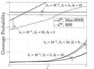
Figure 1: Average coverage probability ${\cal C}^{x}$ vs. $\lambda_{2}$ over $(3,0,0,3)$-order Fox’s ${\mathcal{H}}$ for multipath fading with ${\mathcal{P}}=(0.2,5.5,-,(1.5,0.4,4.5),-,\frac{1}{2}{\bf 1}_{3})$. ${\cal M}=2$, $\alpha=4$, $P_{1}=50$ W, $P_{2}=1$ W, and $\sigma_{1}^{2}=\sigma_{2}^{2}=10^{-6}$, for: (a) both RSS and max-SINR CA schemes and $x=\cal{U}$, and (b) max-SINR CA and $x\in\{\cal{U},\cal{B}\}$..

Figure 2: Average coverage probability ${\cal C}^{x}$ vs. $\lambda_{2}$ over $(3,0,0,3)$-order Fox’s ${\mathcal{H}}$ for multipath fading with ${\mathcal{P}}=(0.2,5.5,-,(1.5,0.4,4.5),-,\frac{1}{2}{\bf 1}_{3})$. ${\cal M}=2$, $\alpha=4$, $P_{1}=50$ W, $P_{2}=1$ W, and $\sigma_{1}^{2}=\sigma_{2}^{2}=10^{-6}$, for: (a) both RSS and max-SINR CA schemes and $x=\cal{U}$, and (b) max-SINR CA and $x\in\{\cal{U},\cal{B}\}$..

V Conclusion

Using a general form, namely the Fox’s $\mathcal{H}$ variate of stochastic variables, we developed a unifying framework to characterize HetNet communication under both RSS and Max-SINR CA rules. Our work systemises the use of the Fox’s $\mathcal{H}$-function to incorporate prominent fading distributions and bounded path-loss models. We proposed generic closed-form expressions for the coverage probability that reveal the actual impact of densification in conjunction with the path-loss model, the fading parameters, and the SINR thresholds.

VI Appendix A: Proof of Proposition 1

Definition 2 (Fox’s ${\mathcal{H}}$ Transform [12]): The ${\mathcal{H}}$-transform of a function $f(x)={\mathcal{H}}_{p_{1},q_{1}}^{m_{1},n_{1}}(x;{\mathcal{P}_{1}}=(\kappa_{1},c_{1},a_{1},b_{1},A_{1},B_{1}))$ is defined by

$$\!\!\!\!\!\!{\mathcal{H}}_{p,q}^{m,n}\left\{f(t);{\mathcal{P}}\right\}(s)\!\!\! = \!\!\!\!\int_{0}^{\infty}\!\!\!\!{\mathcal{H}}_{p,q}^{m,n}(t;{\cal P})f(ts)dt,$$ (17)

$$= \!\!\!\!\frac{1}{s}{\mathcal{H}}_{p+q_{1},q+p_{1}}^{m+n_{1},n+m_{1}}(s^{-1};{\mathcal{P}}\odot{\mathcal{P}_{1}}),$$

where

$${\mathcal{P}}\odot{\mathcal{P}_{1}}\!\!\!\!\! \triangleq \!\!\!\!\!\!\bigg{(}\frac{{\mathcal{\kappa}}{\mathcal{\kappa}}_{1}}{c_{1}},\frac{c}{c_{1}},(1\!-\!b_{1}\!-\!B_{1},a),(b^{1:m},1-a_{1}-A_{1},$$ (18)

$$\!\!\!\!b^{m+1:q}),(B_{1},A),(B^{1:m},A_{1},B^{m+1:q})\!\bigg{)}.$$

Proof: Follows from the Mellin transform of the product of two ${\mathcal{H}}$-functions [12, Eq. (2.3)].

Resorting to [4, Theorem 1] and [5, Eq. (39)] under the independency of $\{\Phi_{j}\}$ and then applying the Fox’s $\mathcal{H}$-transform in (17), we have

$${\cal C}^{\cal U}(r_{k}) = \int_{0}^{\infty}\frac{1}{\sqrt{\xi}}~{}{\cal L}^{-1}\left\{\frac{1}{\sqrt{s}}{\mathcal{H}}_{p,q}^{m,n}\left\{f(t);{\mathcal{P}}\right\}(s\xi);s;{\cal\beta}_{k}\right\}$$ (19)

$$e^{-\sigma^{2}_{k}\xi\frac{r_{k}^{\alpha}}{P_{k}}}\prod_{j\in{\cal M}}{\cal L}_{{\cal I}_{j}}\left(\xi\frac{r_{k}^{\alpha}}{P_{k}}\right)d\xi,$$

where $f(t)=\sqrt{t}{\mathcal{J}}_{1}\left(2\sqrt{st\xi}\right)$, ${\mathcal{J}}_{1}(x)={\mathcal{H}}_{0,2}^{1,0}\left(\frac{x^{2}}{4};(1,1,\frac{1}{2},-\frac{1}{2},1,1)\right)$ is the Bessel function of the first kind [15, Eq. (8.402)], and ${\cal L}^{-1}$ is the inverse Laplace transform. Moreover in (23), ${\cal L}_{{\cal I}_{j}}$ is the Laplace transform of the aggregate interference from the $j$-th tier evaluated as in [5, Eq. (43)] as

$${\cal L}_{{\cal I}_{j}}(\xi)\!=\!\exp\left(\!-\pi\delta\lambda_{j}\frac{\xi r_{k}^{2-\alpha}}{\left(1-\delta\right)}{\mathcal{H}}_{p,q}^{m,n}\left\{g(t);{\mathcal{P}}\right\}(\xi)\!\right),$$ (20)

where $g(t)=t~{}{\rm{}_{2}F_{2}}\left(1,1-\delta;2;2-\delta;-\xi tr^{-\alpha}\right)=t{\mathcal{H}}_{2,3}^{1,2}\left(t;{\cal P}_{1}\right)$, ${\cal P}_{1}=(1-\delta,\xi r^{-\alpha},(0,\delta),(0,-1,\delta-1),{\bf 1}_{2},{\bf 1}_{3})$, and ${\rm{}_{p}F_{q}}(\cdot)$ is the generalized hypergeometric function of [15, Eq. (9.14.1)]. Finally, applying [12, Eq. (1.58)], the ${\mathcal{H}}$-transform in (17) and the inverse Laplace transform of the Fox’s $\mathcal{H}$-function [12, Eq. (2.21)] given by

$${\cal L}^{-1}\{x^{-\rho}{\mathcal{H}}_{p,q}^{m,n}(x;{\cal P});x;t\}=t^{-\rho-1}{\mathcal{H}}_{p+1,q}^{m,n}\left(\frac{1}{t};{\cal P}_{l}\right),$$ (21)

where ${\cal P}_{l}=(\kappa,c,(a,\rho),b,(A,1),B)$, the desired result is obtained after applying the Fox’s ${\mathcal{H}}$ reduction formulae in [12, Eq. (1.57)]. The coverage probability over Fox’s $\mathcal{H}$-fading​ with unbounded path-loss model for a receiver connecting to a $k$-th tier BS located at $x_{k}$ is given by

$${\cal C}^{\cal U}(r_{k})\!\! = \!\!\int_{0}^{\infty}\frac{1}{\xi^{2}}{\mathcal{H}}_{q,p+1}^{n,m}\left(\xi;{\cal P}^{k}_{\cal U}\right)\exp\Bigg{(}-\frac{\sigma^{2}_{k}}{P_{k}}\xi r_{k}^{\alpha}$$ (22)

$$\!\!\!\!\!\!\!\!\!\!\!\!-\pi\delta\sum_{j\in{\cal M}}r_{k}^{2}\lambda_{j}\widetilde{P}_{j}^{\delta}\xi{\mathcal{H}}_{q+2,p+3}^{n+1,m+2}\left(\xi;{\cal P}^{{\cal I}}_{\cal U}\right)\Bigg{)}d\xi,$$

where $\widetilde{P}_{j}=\frac{P_{j}}{P_{k}}$, $\delta=\frac{2}{\alpha}$, and the parameter sequences ${\cal P}^{k}_{\cal U}=\!\!\left(\kappa{\cal\beta}_{k},\frac{1}{c{\cal\beta}_{k}},1\!-\!b,(1\!-\!a,1),\mathcal{B},(A,1)\right),$ and ${\cal P}^{{\cal I}}_{\cal U}=\bigg{(}\frac{\kappa}{c^{2}},\frac{1}{c},(1\!-\!b\!-\!2B,0,\delta),(0,1\!-\!a\!-\!2A,-1,\delta\!-\!1),$ $(\mathcal{B},1,1),(1,A,1,1)\bigg{)}$. Recall under the RSS CA that the PDF of the link’s distance $r_{k}$ in HetNets is given by $f_{r_{k}}(x)=\frac{2\pi\lambda_{k}}{\theta_{k}}x\exp\left(-\sum_{j\in{\cal M}}\pi x^{2}\lambda_{j}\widetilde{P}_{j}^{\delta}\right)$ [1]. Then recognizing that $\exp(-x)={\mathcal{H}}_{0,1}^{1,0}(x;{1,1,0,1,1,1})$ [12, Eq. (1.125)] in (22), we apply (17) to obtain the average coverage probability in (4) after some manipulations.

VII Appendix B: Proof of Proposition 2

The proof of this Proposition relies on the very same approach adopted in Appendix A, yielding

$${\cal C}^{\cal B}(r_{k})\!\!\!\! = \!\!\!\!\int_{0}^{\infty}\frac{1}{\sqrt{\xi}}~{}{\cal L}^{-1}\left\{\frac{1}{\sqrt{s}}{\mathcal{H}}_{p,q}^{m,n}\left\{f(t);{\mathcal{P}}\right\}(s\xi);s;{\cal\beta}_{k}\right\}$$ (23)

$$e^{-\sigma^{2}_{k}\xi\frac{(1+r_{k})^{\alpha}}{P_{k}}}\prod_{j\in{\cal M}}{\cal L}_{{\cal I}_{j}}\left(\xi\frac{(1+r_{k})^{\alpha}}{P_{k}}\right)d\xi,$$

where rearranging [5, Eq. (39)] after carrying out the change of variable relabeling $(1+x)^{-\alpha}$ as $x$, we have

$$\!{\cal L}_{{\cal I}_{j}}(\xi)\!\!\!\! = \!\!\!\!\exp\!\!\Bigg{(}\!\!\!-\pi\delta\lambda_{j}\xi\Bigg{(}\!\!\frac{(1\!+\!r_{k})^{2-\alpha}}{\left(1-\delta\right)}{\mathcal{H}}_{p,q}^{m,n}\!\!\left\{g_{1}(t);{\mathcal{P}_{1}}\right\}(\xi)-$$ (24)

$$\frac{(1+r_{k})^{1-\alpha}}{\left(1-\frac{\delta}{2}\right)}{\mathcal{H}}_{p,q}^{m,n}\left\{g_{2}(t);{\mathcal{P}}\right\}(\xi)\Bigg{)}\Bigg{)},$$

where $g_{1}(t)=t~{}{\rm{}_{2}F_{2}}\left(1,1-\delta;2;2-\delta;-\xi t(1+r_{k})^{-\alpha}\right)$ and $g_{2}(t)=t~{}{\rm{}_{2}F_{2}}\left(1,1-\frac{\delta}{2};2;2-\frac{\delta}{2};-\xi t(1+r_{k})^{-\alpha}\right)$. Finally applying (17) and plugging the obtained result back into (23), Proposition 2 then follows after some manipulations.

VIII Appendix C: Proof of Proposition 3

Referring to [5], the Laplace transform of the ICI from tier $j$ under max-SINR CA is evaluated as ${\cal L}_{{\cal I}_{j}}(\xi)=\exp\left(-\pi\lambda_{j}\xi^{\delta}\Gamma\left(1-\delta\right){\cal E}[H^{\delta}]\right)$, where ${\cal E}[H^{\delta}]$ is the Mellin transform of the Fox’s-${\mathcal{H}}$ function obtained as ${\cal E}[H^{\delta}]=\Lambda^{m,n}_{p,q}$ [12, Eq. (2.8)]. Then following the same lines developed in Appendix A yields

$${\cal C}^{\cal U}(r_{k}) = \int_{0}^{\infty}\frac{1}{\xi^{2}}{\mathcal{H}}_{q,p+1}^{n,m}\left(\xi;{\cal P}^{k}_{\cal U}\right)\exp\Bigg{(}-\frac{\sigma^{2}_{k}}{P_{k}}\xi r_{k}^{\alpha}$$ (25)

$$\!\!\!\!\!\!\!\!\!\!\!\!-\sum_{j\in{\cal M}}r_{k}^{2}\pi\lambda_{j}\widetilde{P}^{\delta}_{j}\left(\frac{\xi}{c}\right)^{\delta}\Gamma(1-\delta)\Lambda^{m,n}_{p,q}\Bigg{)}d\xi.$$

Finally, substituting (25) into (10) and applying (17) along with [12, Eq. (1.59)] yield

$$\!\!\!{\cal C}^{\cal U}\!\!\!\! = \!\!\!\!\!\sum_{k\in{\cal M}}\lambda_{k}{\mathcal{H}}_{1,1}^{1,1}\left(1;\tilde{{\cal P}}_{k}\right)\int_{0}^{\infty}\frac{1}{\xi^{\delta+2}}{\mathcal{H}}_{q,p+1}^{n,m}\left(\xi;{\cal P}^{k}_{\cal U}\right)d\xi$$ (26)

$$= \sum_{k\in{\cal M}}\frac{\lambda_{k}}{\beta_{k}^{\delta}}~{}{\mathcal{H}}_{1,1}^{1,1}\left(1;\tilde{{\cal P}}_{k}\right)\widetilde{\Lambda}^{n,m}_{q,p+1},$$

where

$$\widetilde{\Lambda}^{n,m}_{q,p+1} = \frac{\kappa}{c^{\delta+1}\Gamma(2+\delta)}$$ (27)

$$\!\!\!\!\!\!\!\!\!\!\!\!\!\!\!\!\!\!\!\!\!\!\!\!\!\!\!\!\!\!\frac{\prod_{j=1}^{n}\Gamma\left(1-a_{j}-(1+\delta)A_{j}\right)\prod_{j=1}^{m}\Gamma\left(b_{j}+(1+\delta)B_{j}\right)}{\prod_{j=n+1}^{p}\left(a_{j}+(1+\delta)A_{j}\right)\prod_{j=m+1}^{q}\Gamma\left(1-b_{j}-(1+\delta)A_{j}\right)}$$

$$= \frac{\Lambda^{n,m}_{p,q}}{\Gamma(1+\delta)}.$$

Figure 3: Central Manuscript Submission Cover Page.

References

• [1] C. Li, J. Zhang, J. G. Andrews, and K. B. Letaief, ”Success probability and area spectral efficiency in multiuser MIMO HetNets,” IEEE Trans. Commun., vol. 64, no. 4, pp. 1544-1556, Apr. 2016.
• [2] J. G. Andrews, F. Baccelli, and R. K. Ganti, ”A tractable approach to coverage and rate in cellular networks,” IEEE Trans. Commun., vol. 59, no. 11, pp. 3122-3134, Nov. 2011.
• [3] H. S. Dhillon, R. K. Ganti, F. Baccelli, and J. G. Andrews, ”Modeling and analysis of K-tier downlink heterogeneous cellular networks,” IEEE J. Select. Areas Commun., vol. 30, no. 3, pp. 550–560, Apr. 2012.
• [4] I. Trigui, S. Affes, and B. Liang, ”Unified stochastic geometry modeling and analysis of cellular networks in LOS/NLOS and shadowed fading,” IEEE Trans. Commun., vol. 5, no. 99, pp. 1-16, July 2017.
• [5] I. Trigui and S. Affes, ”Unified analysis and optimization of D2D communications in cellular Networks over fading channels”, IEEE Trans. Commun., early access, July 2018.
• [6] M.G. Khoshkholgh and V. C. M. Leung, ”Coverage analysis of max-SIR cell association in hetNets under nakagami fading”, IEEE Trans. Vehic. Techn., vol. 67, no. 3, pp. 2420-2438. Mar. 2018.
• [7] A. K. Gupta, H. S. Dhillon, S. Vishwanath, and J. G. Andrews, ”Downlink multi-antenna heterogeneous cellular network with load balancing,” IEEE Trans. Commun., vol. 62, no. 11, pp. 4052-4067, Nov. 2014.
• [8] S. K. Yoo, S. Cotton, P. Sofotasios, M. Matthaiou, M. Valkama, and G. Karagiannidis, ”The Fisher-Snedecor F distribution: A simple and accurate composite fading model,” IEEE Commun. Letters, vol. 21, no. 7, pp. 1661-1664, July 2017.
• [9] Y. A. Rahama , M. H. Ismail, and M. S. Hassan, ”On the sum of sndependent Fox’s H-function variates with applications”, IEEE Trans. Vehic. Techn., vol. 67, no. 8, pp. 6752-6760, Aug. 2018.
• [10] Y. J. Chun, S. L. Cotton, H. S. Dhillon, A. Ghrayeb, and M. O. Hasna, ”A stochastic geometric analysis of device-to-device communications operating over generalized fading channels,” IEEE Trans. Wireless Commun., vol. 16, no. 7, pp. 4151-4165, Jul. 2017
• [11] F. Yilmaz and M.-S. Alouini, ”A novel unified expression for the capacity and bit error probability of wireless communication systems over generalized fading channels,” IEEE Trans. Commun., vol. 60, no. 7, pp. 1862-1876, Jul. 2012
• [12] A. M. Mathai, R. K. Saxena, and H. J. Haubol, The H-function: Theory and Applications, Springer Science & Business Media, 2009.
• [13] A. Kilbas and M. Saigo, H-Transforms: Theory and Applications, CRC Press, 2004.
• [14] J. Liu, M. Sheng, L. Liu, and J. Li, ”Effect of densification on cellular network performance with bounded path-loss model,” IEEE Commun. Lett., vol. 21, no. 2, pp. 346-349, Feb. 2017.
• [15] I. S. Gradshteyn and I. M. Ryzhik, Table of Integrals, Series and Products, 5th ed., Academic Publisher, 1994.
Refer to caption