Advisor:	Prof. Carlo Oleari
Co-advisor:	Prof. Paolo Nason
Coordinator:	Prof. Marta Calvi
	Academic year: 2017/2018

Declaration

This dissertation is a result of my own efforts. The work to which it refers is based on my PhD research projects:

1. “A Theoretical Study of Top-Mass Measurements at the LHC Using NLO+PS Generators of Increasing Accuracy,” with T. Ježo, P. Nason and C. Oleari,
   Eur.Phys.J. C78 (2018) no.6, 458 [arXiv:1801.03944v2 [hep-ph]]

2. “All-orders behaviour and renormalons in top-mass observables” with P. Nason and C. Oleari,
   JHEP 1901 (2019) 203 [arXiv:1801.10931 [hep-ph]]

I hereby declare that except where specific reference is made to the work of others, the contents of this dissertation are original and have not been submitted in whole or in part for consideration for any other degree or qualification in this, or any other university.

Silvia Ferrario Ravasio,

31^st October 2018

Abstract

In this thesis we focus on the theoretical subtleties of the top-quark mass ($m_{t}$) determination, issue which persists in being highly controversial.

Typically, in order to infer the top mass, theoretical predictions dependent on $m_{t}$ are employed. The parameter $m_{t}$ is the physical mass, that is connected with the bare mass though a renormalization procedure. Several renormalization schemes are possible and the most natural seems to be the pole-mass one. However, the pole mass is not very well defined for a coloured object like the top quark. The pole mass is indeed affected by the presence of infrared renormalons. They manifest as factorially growing coefficients that spoil the convergence of the perturbative series, leading to ambiguities of order of $\Lambda_{\mathchoice{\displaystyle}{\scriptstyle}{\scriptscriptstyle}{\scriptscriptstyle}\rm QCD}$. On the other hand, short-distance mass schemes, like the $\overline{\rm MS}$, are known to be free from such renormalons. Luckily, the renormalon ambiguity seems to be safely below the quoted systematic errors on the pole-mass determinations, so these measurements are still valuable. In the first part of the thesis, we investigate the presence of linear renormalons in observables that can be employed to determine the top mass. We considered a simplified toy model to describe $W^{*}\rightarrow t\bar{b}\to Wb\bar{b}$. The computation is carried out in the limit of a large number of flavours ($n_{f}$), using a new method that allows to easily evaluate any infrared safe observable at order $\alpha_{\mathchoice{\displaystyle}{\scriptstyle}{\scriptscriptstyle}{\scriptscriptstyle}\rm S}(\alpha_{\mathchoice{\displaystyle}{\scriptstyle}{\scriptscriptstyle}{\scriptscriptstyle}\rm S}n_{f})^{n}$ for any $n$. The observables we consider are, in general, affected by two sources of renormalons: the pole-mass definition and the jet requirements. We compare and discuss the predictions obtained in the usual pole scheme with those computed in the $\overline{\rm MS}$ one. We find that the total cross section without cuts, when expressed in terms of the $\overline{\rm MS}$ mass, does not exhibit linear renormalons, but, as soon as selection cuts are introduced, jet-related linear renormalons arise in any mass scheme. In addition, we show that the reconstructed mass is affected by linear renormalons in any scheme. The average energy of the $W$ boson (that we consider as a simplified example of leptonic observable) has a renormalon in the narrow-width limit in any mass scheme, that is however screened at large orders for finite top widths, provided the top mass is in the $\overline{\rm MS}$ scheme.

The most precise determinations of the top mass are the direct ones, i.e. those that rely upon the reconstruction of the kinematics of the top-decay products. Direct determinations are heavily based on the use of Monte Carlo event generators. The generators employed must be as much accurate as possible, in order not to introduce biases in the measurements. To this purpose, the second part of the thesis is devoted to the comparison of several NLO generators, implemented in the POWHEG BOX framework, that differ by the level of accuracy employed to describe the top decay. The impact of the shower Monte Carlo programs, used to complete the NLO events generated by POWHEG BOX, is also studied. In particular, we discuss the two most widely used shower Monte Carlo programs, i.e. Pythia8.2 and Herwig7.1, and we present a method to interface them with processes that contain decayed emitting resonances. The comparison of several Monte Carlo programs that have formally the same level of accuracy is, indeed, a mandatory step towards a sound estimate of the uncertainty associated with $m_{t}$.

Contents

1. Introduction
2. I Renormalons and all-orders behaviour in top-mass sensitive observables
   1. 1 Introduction
   2. 2 Generalities on divergent series and on the renormalon concept
      1. 2.1 Dyson’s argument
      2. 2.2 Divergent series
      3. 2.3 QCD infrared renormalons
   3. 3 The large-$\boldsymbol{n_{f}}$ limit
      1. 3.1 The dressed gluon propagator
      2. 3.2 Pole-$\overline{\rm MS}$ mass conversion
      3. 3.3 Realistic large-$b_{0}$ approximation
   4. 4 Description of the calculation
      1. 4.1 The ${\Delta\sigma_{q\bar{q}}}$ contribution
      2. 4.2 The ${\sigma_{g^{*}}}$ contribution
         1. 4.2.1 The gluon contribution
         2. 4.2.2 The ${q\bar{q}}$ contribution
         3. 4.2.3 Combination of the gluon and the $q\bar{q}$ contributions
      3. 4.3 The ${\sigma_{\rm v}}$ contribution
      4. 4.4 Combining the virtual and the real contributions
      5. 4.5 Calculation summary
      6. 4.6 Infrared-safe observables
      7. 4.7 Changing the mass scheme
   5. 5 Evaluation of the linear sensitivity in top-mass dependent observables
      1. 5.1 Inclusive cross section
         1. 5.1.1 Selection cuts
         2. 5.1.2 Total cross section without cuts
         3. 5.1.3 Total cross section with cuts
      2. 5.2 Reconstructed-top mass
      3. 5.3 $W$ boson energy
   6. 6 All-order expansions in $\boldsymbol{\alpha_{\mathchoice{\displaystyle}{\scriptstyle}{\scriptscriptstyle}{\scriptscriptstyle}\rm S}}$
      1. 6.1 Mass-conversion formula
      2. 6.2 The total cross section
         1. 6.2.1 Total cross section without cuts
         2. 6.2.2 Total cross section with cuts
      3. 6.3 Reconstructed-top mass
      4. 6.4 ${W}$ boson energy
   7. 7 Summary and conclusions
3. II Top-quark mass extraction with Monte Carlo event generators
   1. 8 Introduction
   2. 9 POWHEG BOX generators for top-pair production
   3. 10 Phenomenological analysis setup
      1. 10.1 Physics objects
      2. 10.2 Methodology
   4. 11 Anatomy of the reconstructed-top mass distribution
      1. 11.1 Les Houches event level comparison of the generators
      2. 11.2 Shower effects
      3. 11.3 Hadronization and underlying events
   5. 12 Reconstructed-top mass distribution
      1. 12.1 $m_{Wb_{j}}^{\max}$ extraction
      2. 12.2 Comparison among different NLO+PS generators
         1. 12.2.1 Matching uncertainties
         2. 12.2.2 Scale, PDF and strong-coupling variations
         3. 12.2.3 Radius dependence
      3. 12.3 Comparison with Herwig7.1
         1. 12.3.1 Alternative settings in Herwig7.1
   6. 13 The energy of the $\boldsymbol{b}$ jet
      1. 13.1 Comparison among different NLO+PS generators
      2. 13.2 Comparison with Herwig7.1
   7. 14 Leptonic observables
   8. 15 Summary and outlook
   9. 16 Conclusions
4. III Appendix
   1. A Radiative corrections to quark lines
      1. A.1 One-loop radiative corrections to heavy quark lines
      2. A.2 Mass counterterm
         1. A.2.1 Non-vanishing gluon mass
         2. A.2.2 Massless gluon
         3. A.2.3 Large gluon mass
      3. A.3 External field normalization
         1. A.3.1 Massless gluon
         2. A.3.2 Massive gluon
      4. A.4 Radiative corrections to external massless quark lines
   2. B A useful dispersive relation
   3. C Single-top production in the narrow-width approximation
      1. C.1 Production cross section
      2. C.2 Top decay width
      3. C.3 Considerations
   4. D Cancellation of the linear sensitivity in the total cross section and in leptonic observables
      1. D.1 Old-fashioned perturbation theory
      2. D.2 Landau singularities
      3. D.3 The specific case
   5. E The POWHEG BOX framework
      1. E.1 NLO computations in the POWHEG BOX (RES)
      2. E.2 NLO events with the POWHEG method
      3. E.3 NLO+PS matching
         1. E.3.1 Interface to shower generators
         2. E.3.2 Pythia8.2
         3. E.3.3 Herwig7.1
   6. F The treatment of remnants for multiple-emission processes
      1. F.1 Sensitivity of the results on hdamp

Introduction

The top quark is the heaviest elementary particle in the Standard Model (SM) that has been observed so far. It thus appears clear that its phenomenology is driven by the large value of its mass $m_{t}$. Indeed, the top is the only quark that decays before hadronizing. This provides us the unique occasion to study the properties of a “bare” quark. For these reasons an accurate determination of $m_{t}$ is part of the Large Hadron Collider (LHC) physics program.

Through radiative corrections, the top-quark mass has a non-negligible impact on many parameters of the Standard Model, like the masses of the electroweak bosons and the Higgs self-coupling. Thus, the value of the $Z$ (or the $W$) mass is sensitive to the value of the top-quark one. For this reason, the electroweak data enable us to have a simultaneous determination of the top and of the $Z$-boson masses and the strong coupling $\alpha_{\mathchoice{\displaystyle}{\scriptstyle}{\scriptscriptstyle}{\scriptscriptstyle}\rm S}(M_{Z})$. The extracted value of $m_{t}$ is $176.7\pm 2.1$ GeV [1], which is in slight tension with the value of $173.34\pm 0.76$ GeV, i.e. the latest Tevatron and the LHC combined results [2]. In addition the top-quark mass is one key ingredient to address the issue of vacuum stability [3, 4, 5, 6]. Under the assumption that there is no new physics up to the Planck scale, the Higgs self coupling $\lambda(\mu)$ is always positive during its renormalization-group flow for each scale $\mu$ adopted, if $m_{t}<171$ GeV. If instead $171<m_{t}<176$ GeV, we are in the metastability region, since $\lambda(\mu)$ becomes negative only at scales of the order of the Planck scale. Thus, there is no indication of new physics below the Planck scale coming from the requirement of vacuum stability.

The most precise determinations of $m_{t}$ are the so called “direct measurements”, which rely upon the full or partial reconstruction of the top momentum out of its decay products. Kinematic distributions sensitive to the top-quark mass are compared to Monte Carlo predictions and the $m_{t}$ value that fits the data the best is the extracted top-quark mass. The ATLAS and CMS measurements of Refs. [7] and [8], yielding the values $m_{t}=172.84\pm 0.34\leavevmode\nobreak\ {\rm(stat)}\pm 0.61$ (syst) GeV and $m_{t}=172.44\pm 0.13\leavevmode\nobreak\ {\rm(stat)}\pm 0.47$ (syst) GeV respectively, fall into this broad category. Of course this kind of determinations is affected by theoretical errors that must be carefully assessed. If the Monte Carlo used to simulate the distributions is not accurate enough, it introduces a bias in the determination of $m_{t}$. For this reason, many efforts have been done in order to implement next-to-leading-order (NLO) generators capable to handle processes containing a decayed emitting resonance, like the top quark is. We will discuss this issue in the second part of the thesis.

However, in contrast with the increasing experimental precision of the top-mass measurements at the LHC, the theoretical interpretation is still matter of debate. In Ref. [9] it was argued that the Monte Carlo mass parameter does not coincide with the top-pole mass and their difference is unavoidable due to the intrinsic ambiguity of the pole-mass definition. Indeed, since the top is quark is always colour-connected with another particle, an isolated top-quark cannot exist. This leads to a renormalon in the relation of the pole to the $\overline{\rm MS}$ mass [10, 11]. Nevertheless, the renormalon ambiguity does not seem severe for the specific case of the top quark, since recent studies [12, 13] have shown that it is in fact well below the current experimental error. In any case non-perturbative corrections to top-mass observables (not necessarily related to the mass renormalon) are present and must be carefully assessed. The top-quark mass renormalon and its interplay with the renormalon arising from the use of jets [14] is discussed in the first part of the thesis.

Part I Renormalons and all-orders behaviour in top-mass sensitive observables

Chapter 1 Introduction

The top mass is measured quite precisely at the LHC by both the ATLAS [15] and the CMS [16] Collaborations. Up to now, the methods that yield the most accurate results are the so called “direct” methods, where kinematic distribution obtained reconstructing fully or partially the top decay products are compared to templates produced with Monte Carlo event generators.

Current uncertainties are now near 500 MeV [7, 8], so that one can worry whether QCD non-perturbative effects may substantially affect the result. In fact, the experimental collaborations estimate these and other effects by varying parameters in the generators, and eventually comparing different generators. This method has been traditionally used in collider physics to estimate theoretical uncertainties due to the modelling of hadronization and underlying events, and also to estimate uncertainties related to higher perturbative orders, as produced by the shower algorithms. We perform a similar study in the second part of the thesis. This is a valuable strategy, as long as all the generators under comparison can reproduce faithfully the data. However, it should not be forgotten that it may only provide a lower bound on the associated errors. However, it should not be forgotten that this statement is true only if all the generators under comparison. It is thus important, at the same time, to investigate the associated uncertainties from a purely theoretical point of view. In consideration of our poor knowledge of non-perturbative QCD, these investigations can at most have a qualitative value, but may help us to understand sources of uncertainties that we might have missed. One such work is presented in Ref. [17], where the authors attempt to relate a theoretically well-defined mass parameter with a corresponding shower Monte Carlo one, using as observable the jet mass of a highly boosted top.

We consider the interplay of non-perturbative effects with the behaviour of perturbative QCD at large orders in the coupling constant, focusing in particular upon observables that, although quite simple, may be considered of the kind used in “direct measurements”.

It is known that, in renormalizable field theories, the renormalization group flow of the couplings leads to the so called renormalons, i.e. to the factorial growth of the coefficients of the perturbative expansion as a function of the order [18, 19, 20, 21, 22, 23, 24, 25]. Renormalons lead to a divergence of the perturbative expansion, that thus becomes asymptotic. In particular, in the case of infrared renormalons in asymptotically-free field theories, the ambiguity in the summation of the series corresponds to a power suppressed effect.

Renormalons were originally found in two-point function diagrams [18, 19, 26]. These contributions are sometimes identified with renormalons in the so-called large (and negative) number of flavour $n_{f}$ limit. We consider a fictitious process $W^{*}\rightarrow t\bar{b}\to Wb\bar{b}$, where the $W$ boson has only a vector coupling to quarks, and examine the behaviour of the cross section, of the reconstructed-top mass and of the energy of the $W$ boson, order by order in the strong coupling expansion, taking the large-$n_{f}$ limit. We consider up to one gluon exchange, or emission, and dress this gluon with an arbitrary number of fermion vacuum-polarization insertions. Furthermore, we also consider final states where the gluon has undergone a splitting into a fermion-antifermion pair, corresponding to a cut vacuum polarization diagram. We assume a finite width for the top quark.

We have devised a method that allowed us to compute in principle any observable in our process, without further approximations, making use of simple numerical techniques. We can thus compute the perturbative expansion at any finite order and infer its asymptotic nature for any observable, with the only limitation of the numerical precision.

We focus for simplicity upon simple top-mass observables, such as the production cross section with or without cuts, the reconstructed-top mass, defined as the mass of a system comprising the $W$ and a $b$ (not $\bar{b}$) jet, and, as a simplified example of leptonic observable, the average value of the energy of the final-state $W$ boson. As discussed earlier, we consider our reconstructed-top mass as an oversimplified representation of observables of the kind used in the so called“direct” measurements. We also stress that we consider the kinematic region where the top energy is not much larger than its mass, that is the region typically used in direct measurements.

We know that there are renormalons arising in the computation of the position of the pole in the top propagators, and we also know that there must be renormalons associated to jets requirements. Since in our framework we can compute the perturbative expansion order by order in perturbation theory, we are in the position to determine explicitly the effects of renormalons in the perturbative expansion.

Our results can be given in terms of the top mass expressed either in the pole or in the $\overline{\rm MS}$ mass scheme. We know that the expression of the pole mass in terms of the $\overline{\rm MS}$ mass has a linear renormalon. If the $\overline{\rm MS}$ mass is considered a fundamental parameter of the theory, this is to be interpreted as an uncertainty of the order of a typical hadronic scale associated to the position of the pole in the top propagator. One may wonder whether the pole mass could instead be used as a fundamental parameter of the theory, which would imply that the $\overline{\rm MS}$ mass has an uncertainty of the order of a hadronic scale. In fact, it is well known and clear (but nevertheless we wish to stress it again) that this last point of view is incorrect. QCD is characterized by a short distance Lagrangian, and its defining parameters are short distance parameters. Thus, if we compute an observable in terms of the $\overline{\rm MS}$ mass, and we find that it has no linear renormalons, we can conclude that the observable has no physical linear renormalons, since its perturbative expansion in terms of the parameters of the short distance Lagrangian has no linear renormalons. On the other end, in the opposite case of an observable that has no linear renormalons if expressed in terms of the pole mass, we must conclude that this observable has a physical renormalon, that is precisely the one that is contained in the pole mass. We also stress that it is the $\overline{\rm MS}$ mass that should enter more naturally in the electroweak fits [1, 27, 28] and in the calculations relative to the stability of the vacuum [3, 4, 5, 6], although in practice the pole mass is often used also in these contexts.

The outline of the first part of the thesis is the following. In Chap. 2 we describe some notions strictly connected with the renormalon issues. In particular we present the physical argument given by Dyson to show that perturbation expansions are not convergent in quantum field theory. We then give a formal definition of asymptotic series and of the Borel transform. In Chap. 3 we discuss the large-$n_{f}$ limit, where higher order corrections are accessible up to all orders in the coupling. As first application, we illustrate the computation of the relation between the pole and the $\overline{\rm MS}$ mass scheme. We also present a possible solution to move from the large-$n_{f}$ limit, that portrays QCD as an Abelian theory, to a more realistic large-$b_{0}$ limit, where $b_{0}$ is the first coefficient of the full QCD $\beta$ function, in order to recover the asymptotic freedom behaviour of the theory. In Chap. 4 we explicitly illustrate the steps for the computation of the fictitious process $W^{*}\rightarrow t\bar{b}\to Wb\bar{b}$ in the large number of flavours limit, using the complex pole mass scheme [29, 30] for the normalization of the top mass. We also show how to rearrange the expression in terms of the $\overline{\rm MS}$ mass, that can be considered as a proxy for all short-distances mass schemes. In Chap. 5 we discuss the presence of infrared linear renormalons in the inclusive cross section, the reconstructed top-mass and the energy of the final-state $W$ boson. We also compare the small-momentum behaviour of such observables computed in the pole scheme with the behaviour achieved by expressing them in terms of a short-distance mass. In Chap. 6 we present the coefficients of the perturbative expansion in $\alpha_{\mathchoice{\displaystyle}{\scriptstyle}{\scriptscriptstyle}{\scriptscriptstyle}\rm S}$ of the above-mentioned observables. Finally, we draw our conclusions in Chap. 7. Some technical details are discussed in Appendices.

The results we present in this first part of the thesis can be found also in Ref. [31].

Chapter 2 Generalities on divergent series and on the renormalon concept

We now illustrate some basic concepts relative to the physics of infrared renormalons.

2.1 Dyson’s argument

Dyson in 1952 showed, with a simple and intuitive physical argument, that perturbative expansions cannot converge in quantum field theory [32].

We can consider, for example,a generic observable in QED given by a perturbation expansion in $e^{2}$:

$$O(e^{2})=\sum_{n=n_{\rm min}}^{\infty}r_{n}\,(e^{2})^{n}.$$ (2.1)

The expansion is performed around the value $e^{2}=0$. If the series converges, then there would be a radius of convergence around $e^{2}=0$. This implies a convergent result also for small and negative values of $e^{2}$. Negative values of $e^{2}$ would correspond to a force that is repulsive for opposite charges and attractive for equal charges. “By creating a large number $N$ of electron-positron pairs, bringing the electrons together in one region of space and the positrons in another separate region, it is easy to construct a “pathological” state in which the negative potential energy of the Coulomb forces is much greater than the total rest energy and kinetic energy of the particles” [32]. This corresponds to a state with unbounded negative energy, that implies the absence of a stable vacuum.

We thus conclude that, since a convergence for negative $e^{2}$ is impossible because the corresponding theory is meaningless, the radius of convergences of the series is zero.

2.2 Divergent series

As we have seen in Sec. 2.1, perturbative series are divergent in quantum field theory. In particular, one may ask whether is possible to assign a “sum” to the series. We consider an observable $O$ written in powers of $\alpha$

$$O\sim\sum_{n=0}^{\infty}c_{n}\alpha^{n+1}.$$ (2.2)

We interpret the series as an asymptotic series in a region $\mathcal{C}$ of the complex $\alpha$-plane if for each order $N$ there are numbers $K_{N}$ that satisfy

$$\left|O-\sum_{n=0}^{N-1}c_{n}\alpha^{n+1}\right|<K_{N}\alpha^{N+1}$$ (2.3)

for all $\alpha$ in $\mathcal{C}$. Let us consider a factorially divergent series

$$c_{n}\xrightarrow{n\to\infty}\mathcal{N}a^{n}\Gamma(1+b+n)\,,$$ (2.4)

with $\mathcal{N}$, $a$ and $b$ constant. When small values of $n$ are concerned, the terms $c_{n}\,\alpha^{n+1}$ decrease for increasing $n$. However, for large values of $n$ the coefficients $c_{n}$ behaves as in (2.4). When a large value $N^{\prime}$ is reached such that

$$\left|c_{N^{\prime}-1}\alpha^{N^{\prime}}\right|\approx\left|c_{N^{\prime}}\alpha^{N^{\prime}+1}\right|,$$ (2.5)

i.e. for

$$N^{\prime}\approx\frac{1}{|a|\alpha},$$ (2.6)

the series of $c_{n}\alpha^{n+1}$ reaches its minimum and then starts growing. The best approximation of the sum of the series is provided when the truncation error is minimum, i.e.

$$c_{N^{\prime}}\alpha^{N^{\prime}+1} = \mathcal{N}\alpha(\alpha\,a)^{\frac{1}{|a|\alpha}}\Gamma\left(1+b+\frac{1}{|a|\alpha}\right)$$ (2.7)

$$\approx \mathcal{N}\alpha\,\left(|a|\alpha\right)^{-b-\frac{1}{2}}\exp\left(-\frac{1}{|a|\alpha}\right)\,.$$

To improve this approximation, we can employ the Borel summation technique. Given the series in eq. (2.2) with $\alpha>0$, its Borel transform is given by

$$B\left[O\right](t)=\sum_{n=0}\frac{c_{n}}{n!}t^{n}$$ (2.8)

and the Borel integral is defined as

$$\widetilde{O}=\int_{0}^{+\infty}\mathrm{d}t\,e^{-t/\alpha}B\left[O\right](t)=\alpha\int_{0}^{+\infty}\mathrm{d}t\,e^{-t}B\left[O\right](\alpha\,t).$$ (2.9)

It can be shown that the Borel integral has the same $\alpha$-expansion of (2.2) and thus, if $\widetilde{O}$ exists, it can be interpreted as the sum of the divergent series. This is particularly useful for alternate sign factorially growing series. We consider the following series and its Borel integral:

$$O=\mathcal{N}\sum_{i=0}^{\infty}a^{n}\,\Gamma(1+b+n)\,\alpha^{n+1}\rightarrow(a\,\alpha)^{-b}\,\frac{\mathcal{N}}{a}\int_{0}^{+\infty}\mathrm{d}t\,e^{-t}\,\Gamma(1+b)\left[\frac{1}{a\,\alpha}-t\right]^{-1-b}.$$ (2.10)

where we have assumed non negative $b$ values. The integral is well defined if $a<0$, i.e. for an alternated-sign series. For positive $a$ values there is a pole on the integration path at $t=-1/a\alpha$. We stress that the location of the pole is independent from the value of $b$. We can give a meaning to the integral by deforming the integration path above or below the pole, that thus acquires an imaginary part equal to

$$\mp\frac{\pi\mathcal{N}}{a}(a\alpha)^{-b}\exp\left(-\frac{1}{a\alpha}\right),$$ (2.11)

where the sign depends on whether the integration is taken in the upper or lower complex plane. The ambiguity can be estimated as $1/2\pi$ times the difference between the two imaginary parts, i.e.

$$\frac{\mathcal{N}}{a}(a\alpha)^{-b}\exp\left(-\frac{1}{a\alpha}\right).$$ (2.12)

By comparing eqs. (2.12) and (2.7) we notice that, in case of same sign factorially divergent series, a small ambiguity proportional to $\exp\left[-1/a\alpha\right]$ is unavoidable.

2.3 QCD infrared renormalons

Infrared renormalons [20, 21] provide a connection between the behaviour of the perturbative expansion at large orders in the coupling constant and non-perturbative effects. They arise when the last loop integration in the $(n+1)$-loop order of the the perturbative expansion acquires the form (see e.g.[24, 25])

$$\alpha_{\mathchoice{\displaystyle}{\scriptstyle}{\scriptscriptstyle}{\scriptscriptstyle}\rm S}^{n+1}(Q)\frac{1}{Q^{p}}\int^{Q}\!\mathrm{d}k\,k^{p-1}\,b_{0}^{n}\,\left(\log\frac{Q^{2}}{k^{2}}\right)^{n}=\frac{n!}{p}\,\left(\frac{2b_{0}}{p}\right)^{n}\alpha_{\mathchoice{\displaystyle}{\scriptstyle}{\scriptscriptstyle}{\scriptscriptstyle}\rm S}^{n+1}(Q)\equiv c_{n}\,\alpha_{\mathchoice{\displaystyle}{\scriptstyle}{\scriptscriptstyle}{\scriptscriptstyle}\rm S}^{n+1}(Q)\,,$$ (2.13)

where $Q$ is the typical scale involved in the process and $b_{0}$ is the first coefficient of the QCD beta function

$$b_{0}=\frac{11\,C_{\mathchoice{\displaystyle}{\scriptstyle}{\scriptscriptstyle}{\scriptscriptstyle}\rm A}}{12\pi}-\frac{n_{f}\,T_{\mathchoice{\displaystyle}{\scriptstyle}{\scriptscriptstyle}{\scriptscriptstyle}\rm R}}{3\pi}\,.$$ (2.14)

The coefficient $b_{0}$ arises because the running coupling is the source of the logarithms in eq. (2.13). A naive justification of the behaviour illustrated in eq. (2.13) can be given by considering the calculation of an arbitrary dimensionless observable, characterized by a scale $Q$, including the effect of the exchange or emission of a single gluon with momentum $k$, leading to a correction that, for small $k$, takes the form

$$\frac{1}{Q^{p}}\int^{Q}\!\mathrm{d}k\,k^{p-1}\alpha_{\mathchoice{\displaystyle}{\scriptstyle}{\scriptscriptstyle}{\scriptscriptstyle}\rm S},$$ (2.15)

where $p$ is an integer greater than zero for the result to be infrared-finite. Assuming that higher order corrections will lead to the replacement of $\alpha_{\mathchoice{\displaystyle}{\scriptstyle}{\scriptscriptstyle}{\scriptscriptstyle}\rm S}$ with the running coupling evaluated at the scale $l$, given by the geometric expansion

$$\alpha_{\mathchoice{\displaystyle}{\scriptstyle}{\scriptscriptstyle}{\scriptscriptstyle}\rm S}(k)=\frac{1}{b_{0}\log\frac{k^{2}}{\Lambda_{\mathchoice{\displaystyle}{\scriptstyle}{\scriptscriptstyle}{\scriptscriptstyle}\rm QCD}^{2}}}=\frac{\alpha_{\mathchoice{\displaystyle}{\scriptstyle}{\scriptscriptstyle}{\scriptscriptstyle}\rm S}(Q)}{1-\alpha_{\mathchoice{\displaystyle}{\scriptstyle}{\scriptscriptstyle}{\scriptscriptstyle}\rm S}(Q)\,b_{0}\log\frac{Q^{2}}{k^{2}}}=\sum_{0}^{\infty}\alpha_{\mathchoice{\displaystyle}{\scriptstyle}{\scriptscriptstyle}{\scriptscriptstyle}\rm S}^{n+1}(Q)\,b_{0}^{n}\,\log^{n}\frac{Q^{2}}{k^{2}}\,,$$ (2.16)

substituting eq. (2.16) into eq. (2.15), we obtain the behaviour of eq. (2.13).

The coefficients of the perturbative expansion displays a factorial growth. The series then is not convergent and can at most be interpreted as an asymptotic series. As anticipated in Sec. 2.2, the terms of the series are smaller and smaller for low values of $n$, until they reach a minimum and then they start to diverge with the order. The minimum is reached when

$$c_{n-1}\,\alpha_{\mathchoice{\displaystyle}{\scriptstyle}{\scriptscriptstyle}{\scriptscriptstyle}\rm S}^{n}(Q)\approx c_{n}\,\alpha_{\mathchoice{\displaystyle}{\scriptstyle}{\scriptscriptstyle}{\scriptscriptstyle}\rm S}^{n+1}(Q)\,,$$ (2.17)

that correspond to $n\approx p/(2b_{0}\alpha_{\mathchoice{\displaystyle}{\scriptstyle}{\scriptscriptstyle}{\scriptscriptstyle}\rm S}(Q))$, and the size of the minimal term is

$$\frac{n!}{p}\left(\frac{2b_{0}}{p}\right)^{n}\alpha_{\mathchoice{\displaystyle}{\scriptstyle}{\scriptscriptstyle}{\scriptscriptstyle}\rm S}^{n+1}(Q) \approx \frac{Q^{p}}{p}\,\alpha_{\mathchoice{\displaystyle}{\scriptstyle}{\scriptscriptstyle}{\scriptscriptstyle}\rm S}(Q)\,n^{-n}\left(n^{n+1/2}e^{-n}\right)$$ (2.18)

$$\approx \alpha_{\mathchoice{\displaystyle}{\scriptstyle}{\scriptscriptstyle}{\scriptscriptstyle}\rm S}(Q)\,\frac{n^{\frac{1}{2}}}{p}\exp\left(-\frac{p}{2\,b_{0}\,\alpha_{\mathchoice{\displaystyle}{\scriptstyle}{\scriptscriptstyle}{\scriptscriptstyle}\rm S}(Q)}\right)\approx\sqrt{\frac{\alpha_{\mathchoice{\displaystyle}{\scriptstyle}{\scriptscriptstyle}{\scriptscriptstyle}\rm S}(Q)}{2b_{0}\,p}}\left(\frac{\Lambda_{\mathchoice{\displaystyle}{\scriptstyle}{\scriptscriptstyle}{\scriptscriptstyle}\rm QCD}}{Q}\right)^{p}\!\!.\qquad$$

If we resum the series whose terms are given in (2.16) using the Borel summation, we will get an ambiguity

$$\frac{1}{2\,b_{0}}\left(\frac{\Lambda_{\mathchoice{\displaystyle}{\scriptstyle}{\scriptscriptstyle}{\scriptscriptstyle}\rm QCD}}{Q}\right)^{p},$$ (2.19)

where we have used eq. (2.12) with $\mathcal{N}=1/p$, $b=0$ and $a=\frac{2b_{0}}{p}$. The value of $p$ depends upon the process under consideration. In this paper, we are interested in linear IR renormalons, corresponding to $p=1$, that can lead to ambiguities in the measured mass of the top quark of relative order $\Lambda_{\mathchoice{\displaystyle}{\scriptstyle}{\scriptscriptstyle}{\scriptscriptstyle}\rm QCD}/m_{t}$, i.e. ambiguities of order $\Lambda_{\mathchoice{\displaystyle}{\scriptstyle}{\scriptscriptstyle}{\scriptscriptstyle}\rm QCD}$ in the top mass. Larger values of $p$ lead to corrections of relative order $\Lambda_{\mathchoice{\displaystyle}{\scriptstyle}{\scriptscriptstyle}{\scriptscriptstyle}\rm QCD}^{p}/m_{t}^{p}$, that are totally negligible.

We will see in Sec. 3 that the behaviour of the perturbative series in eq. (2.13) arises when considering the large number of flavours limit. However, if we include more refinements, the expected behaviour [24, 25] becomes more complicate:

$$c_{n+1}\,\alpha_{\mathchoice{\displaystyle}{\scriptstyle}{\scriptscriptstyle}{\scriptscriptstyle}\rm S}^{n+1}(Q)\propto\Gamma(1+b+n)\left(\frac{2b_{0}}{p}\right)^{n}\alpha_{\mathchoice{\displaystyle}{\scriptstyle}{\scriptscriptstyle}{\scriptscriptstyle}\rm S}^{n+1}(Q)$$ (2.20)

being $b$ a positive number. As we have seen in Sec. 2.2, this does not change the location of the singularity in the Borel plane and still leads to an ambiguity of the resummed series proportional to $\exp\left(-\frac{p}{2\,b_{0}\,\alpha_{\mathchoice{\displaystyle}{\scriptstyle}{\scriptscriptstyle}{\scriptscriptstyle}\rm S}(Q)}\right)\approx\left(\frac{\Lambda_{\mathchoice{\displaystyle}{\scriptstyle}{\scriptscriptstyle}{\scriptscriptstyle}\rm QCD}}{Q}\right)^{p}$. Thus our reasoning is not modified.

Chapter 3 The large-$\boldsymbol{n_{f}}$ limit

The full renormalon structure of QCD is not known. There is however a fully consistent simplified model where higher order corrections are accessible up to all orders in the coupling, namely the large number of flavours, $n_{f}$, limit of QCD. In this limit, the only higer-order contributions that must be considered are the insertion of fermion loops in a gluon propagator, since they involve powers of $n_{f}\alpha_{\mathchoice{\displaystyle}{\scriptstyle}{\scriptscriptstyle}{\scriptscriptstyle}\rm S}$. Examples of computations performed in this limit can be found in Refs. [33, 34].

Unfortunately, the large-$n_{f}$ limit of QCD does not yield to an asymptotically free theory, since the first coefficient of the $\beta$ function would be positive if we neglect self-gauge interactions.

However, it is believed that tracing the fermionic contribution to the $\beta$ function, and, at the end of the computation, making the replacement

$$n_{f}\to-\frac{11C_{\mathchoice{\displaystyle}{\scriptstyle}{\scriptscriptstyle}{\scriptscriptstyle}\rm A}}{4T_{\mathchoice{\displaystyle}{\scriptstyle}{\scriptscriptstyle}{\scriptscriptstyle}\rm R}}+n_{l}\,,$$ (3.1)

where $C_{\mathchoice{\displaystyle}{\scriptstyle}{\scriptscriptstyle}{\scriptscriptstyle}\rm A}=3$, $T_{\mathchoice{\displaystyle}{\scriptstyle}{\scriptscriptstyle}{\scriptscriptstyle}\rm R}=1/2$ and $n_{l}$ is the number of light flavours, one recovers the correct results. In this way, the first coefficient of the $\beta$ function computed in the large-$n_{f}$, $b_{0}$, is matched with its full expression:

$$b_{0}=\frac{11}{3\pi}C_{\mathchoice{\displaystyle}{\scriptstyle}{\scriptscriptstyle}{\scriptscriptstyle}\rm A}-\frac{4}{3\pi}T_{\mathchoice{\displaystyle}{\scriptstyle}{\scriptscriptstyle}{\scriptscriptstyle}\rm F}\,,$$ (3.2)

with $T_{\mathchoice{\displaystyle}{\scriptstyle}{\scriptscriptstyle}{\scriptscriptstyle}\rm F}=T_{\mathchoice{\displaystyle}{\scriptstyle}{\scriptscriptstyle}{\scriptscriptstyle}\rm R}n_{l}$. Since there is no formal proof of this statement, this is just a working hypothesis. Our strategy to retain the full QCD $\beta$ function is slightly different from the one above mentioned and it is described in Sec. 3.3.

3.1 The dressed gluon propagator

In this section we address more technical details about the dressed gluon propagator to all orders in the large-$n_{f}$ limit.

The insertion of an infinite number of self-energy corrections

$$\Pi^{\mu\nu}(k,\mu)=(-g^{\mu\nu}k^{2}+k^{\mu}k^{\nu})\,i\,\Pi(k^{2},\mu^{2})\,,$$ (3.3)

where $i\eta$ is a small imaginary part coming from the Feynman prescription to integrate around the poles, along a gluon propagator of momentum $k$, gives rise to

$$\frac{-i}{k^{2}+i\eta}\,g^{\mu\nu}+\frac{-i}{k^{2}+i\eta}\,\Pi^{\mu\nu}(k,\mu)\,\frac{-i}{k^{2}+i\eta}+\ldots=-\frac{i}{k^{2}+i\eta}\,g^{\mu\nu}\frac{1}{1+\Pi(k^{2},\mu^{2})}\,,$$ (3.4)

where we have dropped all the longitudinal terms. The derivation of the exact $d$-dimensional expression of $\Pi(k^{2},\mu^{2})$ can be found e.g. in Ref. [35]. In the limit of large number of flavours, i.e. considering only light-quark loops, $\Pi(k^{2},\mu^{2})$ is given by

$$\Pi\left(k^{2},\mu^{2}\right) =\frac{\alpha_{\mathchoice{\displaystyle}{\scriptstyle}{\scriptscriptstyle}{\scriptscriptstyle}\rm S}T_{\mathchoice{\displaystyle}{\scriptstyle}{\scriptscriptstyle}{\scriptscriptstyle}\rm F}}{\pi}e^{\epsilon{\gamma_{\mathchoice{\displaystyle}{\scriptstyle}{\scriptscriptstyle}{\scriptscriptstyle}E}}}\frac{\Gamma(1+\epsilon)\,\Gamma^{2}(1-\epsilon)}{\Gamma(1-2\epsilon)}\frac{1-\epsilon}{(3-2\epsilon)(1-2\epsilon)}\,\frac{1}{\epsilon}\left(\frac{-k^{2}}{\mu^{2}}\right)^{-\epsilon},$$ (3.5)

$$=\frac{\alpha_{\mathchoice{\displaystyle}{\scriptstyle}{\scriptscriptstyle}{\scriptscriptstyle}\rm S}T_{\mathchoice{\displaystyle}{\scriptstyle}{\scriptscriptstyle}{\scriptscriptstyle}\rm F}}{\pi}\left[\frac{1}{\epsilon}-\log\left(\frac{-k^{2}}{\mu^{2}}\right)+\frac{5}{3}\right]+\mathcal{O}(\epsilon),$$ (3.6)

where $T_{\mathchoice{\displaystyle}{\scriptstyle}{\scriptscriptstyle}{\scriptscriptstyle}\rm F}=n_{f}T_{\mathchoice{\displaystyle}{\scriptstyle}{\scriptscriptstyle}{\scriptscriptstyle}\rm R}$, ${\gamma_{\mathchoice{\displaystyle}{\scriptstyle}{\scriptscriptstyle}{\scriptscriptstyle}E}}$ is the Euler-Mascheroni constant and we implicitly assume $\alpha_{\mathchoice{\displaystyle}{\scriptstyle}{\scriptscriptstyle}{\scriptscriptstyle}\rm S}=\alpha_{\mathchoice{\displaystyle}{\scriptstyle}{\scriptscriptstyle}{\scriptscriptstyle}\rm S}(\mu)$. Eq. (3.5) can be obtained replacing

$$\mu^{2}\to\mu^{2}\frac{e^{\epsilon{\gamma_{\mathchoice{\displaystyle}{\scriptstyle}{\scriptscriptstyle}{\scriptscriptstyle}E}}}}{4\pi}$$ (3.7)

in eq. (4.21) of Ref. [35], according to the $\overline{\rm MS}$ prescription.

If $k^{2}>0$, we must replace $k^{2}\to k^{2}+i\eta$, where $i\eta$ is a small imaginary part coming from the Feynman prescription. As a consequence, $\Pi(k^{2},\mu^{2})$ develops an imaginary part equal to

$${\rm Im}\,\Pi(k^{2},\mu^{2})=\frac{\alpha_{\mathchoice{\displaystyle}{\scriptstyle}{\scriptscriptstyle}{\scriptscriptstyle}\rm S}T_{\mathchoice{\displaystyle}{\scriptstyle}{\scriptscriptstyle}{\scriptscriptstyle}\rm F}}{3}.$$ (3.8)

The replacement in eq. (3.7) is particularly convenient since it enables us to absorb in the counterterm only the (UV) divergent part of $\Pi$

$$\Pi_{\operatorname{ct}}=\frac{\alpha_{\mathchoice{\displaystyle}{\scriptstyle}{\scriptscriptstyle}{\scriptscriptstyle}\rm S}T_{\mathchoice{\displaystyle}{\scriptstyle}{\scriptscriptstyle}{\scriptscriptstyle}\rm F}}{3\pi}\frac{1}{\epsilon}\,.$$ (3.9)

The renormalized gluon propagator dressed with the sum of all quark-loop insertion is then given by

$$-\frac{i}{k^{2}+i\eta}\,g^{\mu\nu}\frac{1}{1+\Pi(k^{2},\mu^{2})-\Pi_{\operatorname{ct}}}\,,$$ (3.10)

where

$$\Pi(k^{2},\mu^{2})-\Pi_{\operatorname{ct}} = \frac{\alpha_{\mathchoice{\displaystyle}{\scriptstyle}{\scriptscriptstyle}{\scriptscriptstyle}\rm S}T_{\mathchoice{\displaystyle}{\scriptstyle}{\scriptscriptstyle}{\scriptscriptstyle}\rm F}}{3\pi}\left[\frac{5}{3}-\log\left(\frac{|k^{2}|}{\mu^{2}}\right)+i\pi\,\theta(k^{2})\right]+{\cal O}(\epsilon)$$ (3.11)

$$= \alpha_{\mathchoice{\displaystyle}{\scriptstyle}{\scriptscriptstyle}{\scriptscriptstyle}\rm S}\,b_{0,f}\left[\log\left(\frac{|k^{2}|}{\mu^{2}\,e^{C}}\right)-i\pi\theta\left(k^{2}\right)\right]+{\cal O}(\epsilon),$$ (3.12)

and we have defined

$$b_{0,f}\equiv-\frac{T_{\mathchoice{\displaystyle}{\scriptstyle}{\scriptscriptstyle}{\scriptscriptstyle}\rm F}}{3\pi}\,,$$ (3.13)

and $C=5/3$.

Sometimes it is useful to introduce a fictitious light quark mass $m_{q}$ to regulate the behaviour of $\Pi(0,\mu^{2})$. The $\overline{\rm MS}$-renormalized vacuum polarization with a massive quark reads

$$\Pi(k^{2},m_{q}^{2},\mu^{2})-\Pi_{\rm ct}=$$ (3.14)

$$\alpha_{\mathchoice{\displaystyle}{\scriptstyle}{\scriptscriptstyle}{\scriptscriptstyle}\rm S}\,b_{0,f}\times\begin{cases}\displaystyle{\log\left(\frac{\mu^{2}}{m_{q}^{2}}\right)}&k^{2}=0\,,\\[14.22636pt] \displaystyle{\left[\log\left(\frac{\mu^{2}}{m_{q}^{2}}\right)+\frac{5}{3}+\rho-\left(1+\frac{\rho}{2}\right)\sqrt{\rho-1}\left(\pi-2\arctan\sqrt{\rho-1}\right)\right]}&0<k^{2}\leq 4m_{q}^{2},\\[14.22636pt] \displaystyle{\left\{\log\left(\frac{\mu^{2}}{m_{q}^{2}}\right)+\frac{5}{3}+\rho+\left(1+\frac{\rho}{2}\right)\sqrt{1-\rho}\left[\log\bigg{|}\frac{1-\sqrt{1-\rho}}{1+\sqrt{1-\rho}}\bigg{|}+i\pi\theta\left(k^{2}-4m_{q}^{2}\right)\right]\right\}}\\[1.42262pt] &k^{2}<0\,\mbox{ and }k^{2}>4m_{q}^{2},\end{cases}$$

where we have defined

$$\rho=\frac{4\,m_{q}^{2}}{k^{2}}.$$ (3.15)

It develops an imaginary part for $k^{2}>4m_{q}^{2}$ equal to

$${\rm Im}\,\Pi(k^{2},m_{q}^{2},\mu^{2})=\alpha_{\mathchoice{\displaystyle}{\scriptstyle}{\scriptscriptstyle}{\scriptscriptstyle}\rm S}\,b_{0,f}\,\pi\left(1+\frac{\rho}{2}\right)\sqrt{1-\rho}.$$ (3.16)

3.2 Pole-$\overline{\boldsymbol{\rm MS}}$ conversion

As first example, we compute the difference between the pole mass $m$ and the $\overline{\rm MS}$ mass $\overline{m}(\mu)$ at all orders in $\alpha_{\mathchoice{\displaystyle}{\scriptstyle}{\scriptscriptstyle}{\scriptscriptstyle}\rm S}(\alpha_{\mathchoice{\displaystyle}{\scriptstyle}{\scriptscriptstyle}{\scriptscriptstyle}\rm S}n_{f})^{n}$. The coupling $\alpha_{\mathchoice{\displaystyle}{\scriptstyle}{\scriptscriptstyle}{\scriptscriptstyle}\rm S}$ is always meant to be evaluated at the scale $\mu$.

At $\mathcal{O}(\alpha_{\mathchoice{\displaystyle}{\scriptstyle}{\scriptscriptstyle}{\scriptscriptstyle}\rm S})$, the self-energy correction evaluated for the eigenvalue of $\not{p}$ equal to $m$ takes the form

$${i\,\Sigma^{(1)}(m,m)}=-i\,g^{2}\,C_{\mathchoice{\displaystyle}{\scriptstyle}{\scriptscriptstyle}{\scriptscriptstyle}\rm F}\left(\frac{\mu^{2}}{4\pi}{\rm e}^{{\gamma_{\mathchoice{\displaystyle}{\scriptstyle}{\scriptscriptstyle}{\scriptscriptstyle}E}}}\right)^{\epsilon}\int\frac{\mathrm{d}^{d}k}{(2\pi)^{d}}\frac{\gamma^{\alpha}(\not{p}+\not{k}+m)\gamma_{\alpha}}{\left[k^{2}+i\eta\right]\left[(k+p)^{2}-m^{2}+i\eta\right]}\Bigg{|}_{\not{p}=m}\,,$$ (3.17)

being $k$ the gluon momentum. The details of computation of $\Sigma^{(1)}(m,m)$ can be found in Appendix  A.2.2 and the result is given by eq. (A.36). The mass counterterms defined in the pole and in the $\overline{\rm MS}$ schemes (see Sec. A) are given by

$$m^{c} = -i\,\Sigma^{(1)}\!\left(m,m\right)$$ (3.18)

$$= -\frac{\alpha_{\mathchoice{\displaystyle}{\scriptstyle}{\scriptscriptstyle}{\scriptscriptstyle}\rm S}}{4\pi}\,C_{\mathchoice{\displaystyle}{\scriptstyle}{\scriptscriptstyle}{\scriptscriptstyle}\rm F}\,e^{\epsilon{\gamma_{\mathchoice{\displaystyle}{\scriptstyle}{\scriptscriptstyle}{\scriptscriptstyle}E}}}\,\Gamma(\epsilon)\,m\,\left(\frac{\mu^{2}}{m^{2}}\right)^{\epsilon}\,\frac{3-2\epsilon}{1-2\epsilon}$$

$$= -\frac{\alpha_{\mathchoice{\displaystyle}{\scriptstyle}{\scriptscriptstyle}{\scriptscriptstyle}\rm S}}{4\pi}\,C_{\mathchoice{\displaystyle}{\scriptstyle}{\scriptscriptstyle}{\scriptscriptstyle}\rm F}\,m\,\left[\frac{3}{\epsilon}+3\log\left(\frac{\mu^{2}}{m^{2}}\right)+4\right]\,+\mathcal{O}(\epsilon)\,,$$

$$\overline{m}^{c}(\mu) = \left[-i\,\Sigma^{(1)}\!\left(\overline{m}(\mu),\overline{m}(\mu)\right)\right]^{\rm(d)}$$ (3.19)

$$= -\frac{\alpha_{\mathchoice{\displaystyle}{\scriptstyle}{\scriptscriptstyle}{\scriptscriptstyle}\rm S}}{4\pi}\,C_{\mathchoice{\displaystyle}{\scriptstyle}{\scriptscriptstyle}{\scriptscriptstyle}\rm F}\,\overline{m}^{c}(\mu)\,\frac{3}{\epsilon},$$

respectively, where (d) denotes the divergent part according to the $\overline{\rm MS}$ definition. Neglecting terms of the order $\alpha_{\mathchoice{\displaystyle}{\scriptstyle}{\scriptscriptstyle}{\scriptscriptstyle}\rm S}^{2}$, the mass difference is given by the finite part of $i\,\Sigma^{(1)}\!\left(m,m\right)$:

$$m-\overline{m}(\mu)=\left[i\,\Sigma^{(1)}\!\left(m,m\right)\right]^{\rm(f)}=\frac{\alpha_{\mathchoice{\displaystyle}{\scriptstyle}{\scriptscriptstyle}{\scriptscriptstyle}\rm S}}{4\pi}\,C_{\mathchoice{\displaystyle}{\scriptstyle}{\scriptscriptstyle}{\scriptscriptstyle}\rm F}\,m\,\left[3\log\left(\frac{\mu^{2}}{m^{2}}\right)+4\right]\,.$$ (3.20)

According to Sec. A, to evaluate $m-\overline{m}(\mu)$ beyond NLO, we need to compute

$$i\Sigma(\not{p},m_{b})\Big{|}_{\not{p}=m}\,,\quad i\Sigma(\not{p},m_{b})\Big{|}_{\not{p}=\overline{m}(\mu)},$$ (3.21)

being $m_{b}$ the bare mass. Since up to $\alpha_{\mathchoice{\displaystyle}{\scriptstyle}{\scriptscriptstyle}{\scriptscriptstyle}\rm S}$ corrections

$$m_{b}\approx m\approx\overline{m}(\mu)$$ (3.22)

and $\Sigma(\not{p},m_{b})$ already contains a factor $\alpha_{\mathchoice{\displaystyle}{\scriptstyle}{\scriptscriptstyle}{\scriptscriptstyle}\rm S}$, in the large-$n_{f}$ limit we can just calculate

$$i\Sigma(\not{p},m)\Big{|}_{\not{p}=m}=i\Sigma(m,m).$$ (3.23)

Indeed, if we replace $m$ with $m_{b}$ or $\overline{m}(\mu)$ in contributions that are $\mathcal{O}(\alpha_{\mathchoice{\displaystyle}{\scriptstyle}{\scriptscriptstyle}{\scriptscriptstyle}\rm S})$, we produce variations of the order $\alpha_{\mathchoice{\displaystyle}{\scriptstyle}{\scriptscriptstyle}{\scriptscriptstyle}\rm S}^{2}(\alpha_{\mathchoice{\displaystyle}{\scriptstyle}{\scriptscriptstyle}{\scriptscriptstyle}\rm S}n_{f})^{n}$, that are totally negligible in our context.

The all-orders expression of $i\,\Sigma(m,m)$ is obtained by replacing the free gluon propagator of eq. (3.17) with the dressed one, as shown in eq. (3.4). We thus obtain

$${i\,\Sigma(m,m)}=-i\,g^{2}\,C_{\mathchoice{\displaystyle}{\scriptstyle}{\scriptscriptstyle}{\scriptscriptstyle}\rm F}\left(\frac{\mu^{2}}{4\pi}{\rm e}^{{\gamma_{\mathchoice{\displaystyle}{\scriptstyle}{\scriptscriptstyle}{\scriptscriptstyle}E}}}\right)^{\epsilon}\int\frac{\mathrm{d}^{d}k}{(2\pi)^{d}}\frac{\gamma^{\alpha}(\not{p}+\not{k}+m)\gamma_{\alpha}}{k^{2}\left[(k+p)^{2}-m^{2}\right]}\frac{1}{1+\Pi(k^{2},\mu^{2})-\Pi_{\rm ct}}\Bigg{|}_{\not{p}=m}.$$ (3.24)

By using eq. (B.10), we can write

$$i\,\Sigma(m,m)=-\frac{i}{\pi}\int_{0^{-}}^{+\infty}\mathrm{d}\lambda^{2} \left\{-\,g^{2}\,C_{\mathchoice{\displaystyle}{\scriptstyle}{\scriptscriptstyle}{\scriptscriptstyle}\rm F}\left(\frac{\mu^{2}}{4\pi}{\rm e}^{{\gamma_{\mathchoice{\displaystyle}{\scriptstyle}{\scriptscriptstyle}{\scriptscriptstyle}E}}}\right)^{\epsilon}\int\frac{\mathrm{d}^{d}k}{(2\pi)^{d}}\frac{\gamma^{\alpha}(\not{p}+\not{k}+m)\gamma_{\alpha}}{\left[k^{2}-\lambda^{2}\right]\left[(k+p)^{2}-m^{2}\right]}\right\}$$

$$\times{\rm Im}\left[\frac{1}{\lambda^{2}}\,\frac{1}{1+\Pi(\lambda^{2},\mu^{2})-\Pi_{\operatorname{ct}}}\right]$$ (3.25)

where we set $m_{q}=0$ since IR divergences are absent. The expression in the curly brackets of eq. (3.25) is the one-loop self-energy of a quark of mass $m$, computed with a gluon of mass $\lambda$, that we denote by $\Sigma^{(1)}_{\lambda}(m,m)$, whose $\mathcal{O}(\epsilon)$ expression is given in eq. (A.28). For ease of notation we introduce

$$\widetilde{r}(\epsilon,\lambda) = \frac{i\,\Sigma^{(1)}_{\lambda}(m,m)}{m}\;=\;\frac{\alpha_{\mathchoice{\displaystyle}{\scriptstyle}{\scriptscriptstyle}{\scriptscriptstyle}\rm S}}{4\pi}C_{\mathchoice{\displaystyle}{\scriptstyle}{\scriptscriptstyle}{\scriptscriptstyle}\rm F}\left[\frac{3}{\epsilon}+3\log\left(\frac{\mu^{2}}{m^{2}}\right)+4\right.$$ (3.26)

$$\left.\hskip 14.22636pt+\frac{\lambda^{2}}{m^{2}}\left(1+\log\left(\frac{\lambda^{2}}{m^{2}}\right)\right)+\left(2+\frac{\lambda^{2}}{m^{2}}\right)H\left(\frac{\lambda^{2}}{m^{2}}\right)\right]+\mathcal{O}(\epsilon)\,,\phantom{aaaa}$$

$$\widetilde{r}(\epsilon,0) = \frac{i\,\Sigma^{(1)}_{0}(m,m)}{m}=\frac{\alpha_{\mathchoice{\displaystyle}{\scriptstyle}{\scriptscriptstyle}{\scriptscriptstyle}\rm S}}{4\pi}\,C_{\mathchoice{\displaystyle}{\scriptstyle}{\scriptscriptstyle}{\scriptscriptstyle}\rm F}\,e^{\epsilon{\gamma_{\mathchoice{\displaystyle}{\scriptstyle}{\scriptscriptstyle}{\scriptscriptstyle}E}}}\,\Gamma(\epsilon)\,\left(\frac{\mu^{2}}{m^{2}}\right)^{\epsilon}\frac{3-2\epsilon}{1-2\epsilon}\,,$$ (3.27)

$$\widetilde{r}^{\infty}(\epsilon,\lambda) = \frac{i\,\Sigma^{(1)}_{\lambda_{\infty}}(m,m)}{m}=\frac{\alpha_{\mathchoice{\displaystyle}{\scriptstyle}{\scriptscriptstyle}{\scriptscriptstyle}\rm S}}{4\pi}\,C_{\mathchoice{\displaystyle}{\scriptstyle}{\scriptscriptstyle}{\scriptscriptstyle}\rm F}\,e^{\epsilon{\gamma_{\mathchoice{\displaystyle}{\scriptstyle}{\scriptscriptstyle}{\scriptscriptstyle}E}}}\,\Gamma(\epsilon)\,\left(\frac{\mu^{2}}{\lambda^{2}}\right)^{\epsilon}\frac{2(3-2\epsilon)}{(1-\epsilon)(2-\epsilon)}\,,$$ (3.28)

where the function $H$ is defined in eq. (A.25) and we have used the expressions of $\Sigma^{(1)}_{\lambda}(m,m)$, $\Sigma^{(1)}_{0}(m,m)$ and $\Sigma_{\lambda_{\infty}}^{(1)}(m,m)$ given by eqs (A.28), (A.35) and (A.46). The parametric dependence on $m$, $\mu$ and $\alpha_{\mathchoice{\displaystyle}{\scriptstyle}{\scriptscriptstyle}{\scriptscriptstyle}\rm S}$ of the integrand functions $\widetilde{r}(\epsilon,\lambda)$, $\widetilde{r}(\epsilon,0)$ and $\widetilde{r}^{\infty}(\epsilon,\lambda)$ is kept implicit for ease of notation. We thus have

$$\frac{i\,\Sigma(m,m)}{m}=-\frac{1}{\pi}\int_{0^{-}}^{+\infty}\mathrm{d}\lambda^{2}\,\widetilde{r}(\epsilon,\lambda)\times{\rm Im}\left[\frac{1}{\lambda^{2}+i\eta}\,\frac{1}{1+\Pi(\lambda^{2},\mu^{2})-\Pi_{\operatorname{ct}}}\right].$$ (3.29)

Since $\widetilde{r}(\epsilon,\lambda)$ contains a single pole in $\epsilon$ and does not vanish for large $\lambda$, we need to evaluate the integrand in $d=4-2\epsilon$ dimensions, in order to extract its finite part. We can express $\widetilde{r}(\epsilon,\lambda)$ as the sum of the following two terms

$$\widetilde{r}_{d}\!\left(\epsilon,\lambda\right) = \frac{\mu^{2}}{\mu^{2}+\lambda^{2}}\,\widetilde{r}(\epsilon,0)+\frac{\lambda^{2}}{\mu^{2}+\lambda^{2}}\,\widetilde{r}^{\infty}\!\left(\epsilon,\lambda\right)\,,$$ (3.30)

$$\widetilde{r}_{f}\!\left(\lambda\right) = \widetilde{r}\!\left(\epsilon,\lambda\right)-\widetilde{r}_{d}\!\left(\epsilon,\lambda\right).$$ (3.31)

We dropped the $\epsilon$ dependence in $\widetilde{r}_{f}$ since we can safely perform the $\epsilon\to 0$ limit, indeed it does not contain any UV $\epsilon$-pole and

$$\lim_{\lambda\to\infty}\widetilde{r}_{f}\!\left(\lambda\right) = \mathcal{O}\left(\frac{m^{2}}{\lambda^{2}}\right)\,,$$ (3.32)

$$\lim_{\lambda\to 0}\widetilde{r}_{f}\!\left(\lambda\right) = -\alpha_{\mathchoice{\displaystyle}{\scriptstyle}{\scriptscriptstyle}{\scriptscriptstyle}\rm S}\frac{C_{\mathchoice{\displaystyle}{\scriptstyle}{\scriptscriptstyle}{\scriptscriptstyle}\rm F}}{2}\frac{\lambda}{m}+\mathcal{O}\left(\frac{\lambda^{2}}{m^{2}}\right)\,,$$ (3.33)

so that we can write

$$\widetilde{r}_{f}\!\left(\lambda\right) = \frac{\alpha_{\mathchoice{\displaystyle}{\scriptstyle}{\scriptscriptstyle}{\scriptscriptstyle}\rm S}C_{\mathchoice{\displaystyle}{\scriptstyle}{\scriptscriptstyle}{\scriptscriptstyle}\rm F}}{4\pi}\left\{-3\log\!\left(\frac{m^{2}}{\mu^{2}}\right)+\frac{\lambda^{2}}{m^{2}}\left(1+\log\frac{\lambda^{2}}{m^{2}}\right)+4+\left(2+\frac{\lambda^{2}}{m^{2}}\right)H\left(\frac{\lambda^{2}}{m^{2}}\right)\right.$$ (3.34)

$$\left.-\frac{\mu^{2}}{\mu^{2}+\lambda^{2}}\,\left[-3\log\!\left(\frac{m^{2}}{\mu^{2}}\right)+4\right]-\frac{\lambda^{2}}{\mu^{2}+\lambda^{2}}\,\left[-3\log\!\left(\frac{\lambda^{2}}{\mu^{2}}\right)+\frac{5}{2}\right]\right\}\,.\phantom{aaaaa}$$

We thus rewrite eq. (3.29) as

$$\frac{i\,\Sigma(m,m)}{m} =r_{f}(m,\mu,\alpha_{\mathchoice{\displaystyle}{\scriptstyle}{\scriptscriptstyle}{\scriptscriptstyle}\rm S})+r_{d}(m,\mu,\alpha_{\mathchoice{\displaystyle}{\scriptstyle}{\scriptscriptstyle}{\scriptscriptstyle}\rm S})\,,$$ (3.35)

$$r_{f}(m,\mu,\alpha_{\mathchoice{\displaystyle}{\scriptstyle}{\scriptscriptstyle}{\scriptscriptstyle}\rm S}) \equiv-\frac{1}{\pi}\int_{0-}^{\infty}\mathrm{d}\lambda^{2}\,\widetilde{r}_{f}\!\left(\lambda\right){\rm Im}\left[\frac{1}{\lambda^{2}+i\eta}\,\frac{1}{1+\Pi(\lambda^{2},\mu^{2})-\Pi_{\operatorname{ct}}}\right],$$ (3.36)

$$r_{d}(m,\mu,\alpha_{\mathchoice{\displaystyle}{\scriptstyle}{\scriptscriptstyle}{\scriptscriptstyle}\rm S}) \equiv-\frac{1}{\pi}\int_{0-}^{\infty}\mathrm{d}\lambda^{2}\,\widetilde{r}_{d}\!\left(\epsilon,\lambda\right){\rm Im}\left[\frac{1}{\lambda^{2}+i\eta}\,\frac{1}{1+\Pi(\lambda^{2},\mu^{2})-\Pi_{\operatorname{ct}}}\right],$$ (3.37)

where we have made explicit the dependence on $m$, $\mu$ and $\alpha_{\mathchoice{\displaystyle}{\scriptstyle}{\scriptscriptstyle}{\scriptscriptstyle}\rm S}$ of the terms $r_{f}(m,\mu,\alpha_{\mathchoice{\displaystyle}{\scriptstyle}{\scriptscriptstyle}{\scriptscriptstyle}\rm S})$ and $r_{d}(m,\mu,\alpha_{\mathchoice{\displaystyle}{\scriptstyle}{\scriptscriptstyle}{\scriptscriptstyle}\rm S})$.

We manipulate $r_{f}(m,\mu,\alpha_{\mathchoice{\displaystyle}{\scriptstyle}{\scriptscriptstyle}{\scriptscriptstyle}\rm S})$ as follows. The lower boundary can be moved from $0^{-}$ to $0$, since $\widetilde{r}_{f}(0)=0$. We also have

$$\frac{1}{\lambda^{2}+i\eta}\,\frac{1}{1+\Pi(\lambda^{2},\mu^{2})-\Pi_{\operatorname{ct}}}=\frac{1}{\alpha_{\mathchoice{\displaystyle}{\scriptstyle}{\scriptscriptstyle}{\scriptscriptstyle}\rm S}\,b_{0,f}}\,\frac{\mathrm{d}\ }{\mathrm{d}\lambda^{2}}\log\left[1+\Pi\left(\lambda^{2},\mu^{2}\right)-\Pi_{\operatorname{ct}}\right],$$ (3.38)

so that

$$r_{f}(m,\mu,\alpha_{\mathchoice{\displaystyle}{\scriptstyle}{\scriptscriptstyle}{\scriptscriptstyle}\rm S})= -\frac{1}{\alpha_{\mathchoice{\displaystyle}{\scriptstyle}{\scriptscriptstyle}{\scriptscriptstyle}\rm S}\,b_{0,f}}\int_{0}^{\infty}\frac{\mathrm{d}\lambda}{\pi}\,\widetilde{r}_{f}\!\left(\lambda^{2}\right){\rm Im}\left\{\,\frac{\mathrm{d}\ }{\mathrm{d}\lambda^{2}}\log\left[1+\Pi\left(\lambda^{2},\mu^{2}\right)-\Pi_{\operatorname{ct}}\right]\right\}$$

$$= \frac{1}{\alpha_{\mathchoice{\displaystyle}{\scriptstyle}{\scriptscriptstyle}{\scriptscriptstyle}\rm S}\,b_{0,f}}\int_{0}^{\infty}\frac{\mathrm{d}\lambda}{\pi}\,\frac{\mathrm{d}\ }{\mathrm{d}\lambda}\left[\widetilde{r}_{f}\!\left(\lambda\right)\right]{\rm Im}\left\{\log\left[1+\Pi\left(\lambda^{2},\mu^{2}\right)-\Pi_{\operatorname{ct}}\right]\right\}\qquad$$

$$= -\frac{1}{\alpha_{\mathchoice{\displaystyle}{\scriptstyle}{\scriptscriptstyle}{\scriptscriptstyle}\rm S}\,b_{0,f}}\int_{0}^{\infty}\frac{\mathrm{d}\lambda}{\pi}\,\frac{\mathrm{d}\ }{\mathrm{d}\lambda}\left[\widetilde{r}_{f}\!\left(\lambda\right)\right]\arctan\left[\frac{\alpha_{\mathchoice{\displaystyle}{\scriptstyle}{\scriptscriptstyle}{\scriptscriptstyle}\rm S}\,\pi\,b_{0,f}}{1+\alpha_{\mathchoice{\displaystyle}{\scriptstyle}{\scriptscriptstyle}{\scriptscriptstyle}\rm S}\,b_{0,f}\,\log\left(\frac{\lambda^{2}}{\mu^{2}e^{C}}\right)}\right],$$ (3.39)

that can be evaluated numerically. We notice that $r_{f}(m,\mu,\alpha_{\mathchoice{\displaystyle}{\scriptstyle}{\scriptscriptstyle}{\scriptscriptstyle}\rm S})$ contains a linear infrared renormalon since the behaviour of $\widetilde{r}_{f}(\lambda)$ for small $\lambda$ is given by eq. 3.33.

As far as the integral in eq. (3.37) is concerned, we can split it into two terms, according to eq. (3.30),

$$r_{d}(m,\mu,\alpha_{\mathchoice{\displaystyle}{\scriptstyle}{\scriptscriptstyle}{\scriptscriptstyle}\rm S})= r_{d}^{0}(m,\mu,\alpha_{\mathchoice{\displaystyle}{\scriptstyle}{\scriptscriptstyle}{\scriptscriptstyle}\rm S})+r_{d}^{\infty}(m,\mu,\alpha_{\mathchoice{\displaystyle}{\scriptstyle}{\scriptscriptstyle}{\scriptscriptstyle}\rm S})\,,$$ (3.40)

$$r_{d}^{0}(m,\mu,\alpha_{\mathchoice{\displaystyle}{\scriptstyle}{\scriptscriptstyle}{\scriptscriptstyle}\rm S})\equiv -\frac{1}{\pi}\int_{0-}^{\infty}\mathrm{d}\lambda^{2}\,\frac{\mu^{2}}{\mu^{2}+\lambda^{2}}\,\widetilde{r}(\epsilon,0)\,{\rm Im}\left[\frac{1}{\lambda^{2}+i\eta}\,\frac{1}{1+\Pi(\lambda^{2},\mu^{2})-\Pi_{\operatorname{ct}}}\right],$$ (3.41)

$$\!\!\!r_{d}^{\infty}(m,\mu,\alpha_{\mathchoice{\displaystyle}{\scriptstyle}{\scriptscriptstyle}{\scriptscriptstyle}\rm S})\equiv -\frac{1}{\pi}\int_{0^{-}}^{\infty}\mathrm{d}\lambda^{2}\,\frac{\lambda^{2}}{\mu^{2}+\lambda^{2}}\,\widetilde{r}^{\infty}\!\left(\epsilon,\lambda\right)\,{\rm Im}\left[\frac{1}{\lambda^{2}+i\eta}\,\frac{1}{1+\Pi(\lambda^{2},\mu^{2})-\Pi_{\operatorname{ct}}}\right].\!\!\!$$ (3.42)

Since the integrand function in $r_{d}^{0}(m,\mu,\alpha_{\mathchoice{\displaystyle}{\scriptstyle}{\scriptscriptstyle}{\scriptscriptstyle}\rm S})$ vanishes for large $\lambda$, the integral of the imaginary part can be replaced with the closed path integral depicted in Fig. B.1. Applying the residue theorem, we have

$$r_{d}^{0}(m,\mu,\alpha_{\mathchoice{\displaystyle}{\scriptstyle}{\scriptscriptstyle}{\scriptscriptstyle}\rm S})=\widetilde{r}(\epsilon,0)\,\frac{1}{1+\Pi(-\mu^{2},\mu^{2})-\Pi_{\operatorname{ct}}}=\widetilde{r}(\epsilon,0)\sum_{n=0}^{\infty}\Big{[}\Pi_{\operatorname{ct}}-\Pi\left(-\mu^{2},\mu^{2}\right)\Big{]}^{n}.$$ (3.43)

In order to deal with the integral in $r_{d}^{\infty}(m,\mu,\alpha_{\mathchoice{\displaystyle}{\scriptstyle}{\scriptscriptstyle}{\scriptscriptstyle}\rm S})$, we need to expose the $\lambda$ dependence of the integrand. From eq. (3.28), we can write

$$\widetilde{r}^{\infty}\!\left(\epsilon,\lambda\right)=\left(\frac{\lambda^{2}}{\mu^{2}}\right)^{\epsilon}R^{\infty}(\epsilon)\,,$$ (3.44)

where $R^{\infty}(\epsilon)$ depends only on $\epsilon$ and no longer on $\lambda$. Similarly, using eq. (3.5), we have

$$\Pi\left(\lambda^{2},\mu^{2}\right) = \frac{\alpha_{\mathchoice{\displaystyle}{\scriptstyle}{\scriptscriptstyle}{\scriptscriptstyle}\rm S}T_{\mathchoice{\displaystyle}{\scriptstyle}{\scriptscriptstyle}{\scriptscriptstyle}\rm F}}{\pi}e^{\epsilon{\gamma_{\mathchoice{\displaystyle}{\scriptstyle}{\scriptscriptstyle}{\scriptscriptstyle}E}}}\frac{\Gamma(1+\epsilon)\,\Gamma^{2}(1-\epsilon)}{\Gamma(1-2\epsilon)}\frac{1-\epsilon}{(3-2\epsilon)(1-2\epsilon)}\,\frac{1}{\epsilon}\left(\frac{\lambda^{2}}{\mu^{2}}\right)^{-\epsilon}e^{i\epsilon\pi}$$ (3.45)

$$= \Pi\left(-\mu^{2},\mu^{2}\right)\left(\frac{\lambda^{2}}{\mu^{2}}\right)^{-\epsilon}e^{i\epsilon\pi},$$

and performing a Taylor expansion we can write

$$\!\!\!\!\!\!\!r_{d}^{\infty}(m,\mu,\alpha_{\mathchoice{\displaystyle}{\scriptstyle}{\scriptscriptstyle}{\scriptscriptstyle}\rm S})=-\frac{R^{\infty}(\epsilon)}{\pi}\int_{0}^{\infty}\mathrm{d}\lambda^{2}\,\frac{1}{\mu^{2}+\lambda^{2}}\left(\frac{\lambda^{2}}{\mu^{2}}\right)^{-\epsilon}\,{\rm Im}\left[\frac{1}{1+\Pi(\lambda^{2},\mu^{2})-\Pi_{\operatorname{ct}}}\right]$$

$$=-\frac{R^{\infty}(\epsilon)}{\pi}\,\sum_{n=0}^{\infty}\,\int_{0}^{\infty}\mathrm{d}\lambda^{2}\,\frac{1}{\mu^{2}+\lambda^{2}}\left(\frac{\lambda^{2}}{\mu^{2}}\right)^{-\epsilon}\,{\rm Im}\left[\Pi_{\operatorname{ct}}-\Pi\left(-\mu^{2},\mu^{2}\right)\left(\frac{\lambda^{2}}{\mu^{2}}\right)^{-\epsilon}e^{i\epsilon\pi}\right]^{n}$$

$$=-\frac{R^{\infty}(\epsilon)}{\pi}\,\sum_{n=1}^{\infty}\,\int_{0}^{\infty}\mathrm{d}z\,\frac{z^{-\epsilon}}{1+z}\,{\rm Im}\Big{[}\Pi_{\operatorname{ct}}-\Pi\left(-\mu^{2},\mu^{2}\right)z^{-\epsilon}e^{i\epsilon\pi}\Big{]}^{n}\,.$$ (3.46)

By computing the imaginary part of the $n$-th power of the term in the square brackets, we are let to evaluate integrals of the form

$$\int_{0}^{\infty}\mathrm{d}z\frac{z^{-h}}{1+z}=\Gamma(1-h)\,\Gamma(h),$$ (3.47)

where $h$ is a real number, so that $r_{d}^{\infty}(m,\mu,\alpha_{\mathchoice{\displaystyle}{\scriptstyle}{\scriptscriptstyle}{\scriptscriptstyle}\rm S})$ can be straightforwardly evaluated by computer algebraic means at any fixed order in $\alpha_{\mathchoice{\displaystyle}{\scriptstyle}{\scriptscriptstyle}{\scriptscriptstyle}\rm S}$. We emphasize that $r_{d}(m,\mu,\alpha_{\mathchoice{\displaystyle}{\scriptstyle}{\scriptscriptstyle}{\scriptscriptstyle}\rm S})$ has no linear renormalon. Indeed if we perform an $\epsilon$ expansion and we consider the small-$\lambda$ contribution, by writing $\mathrm{d}\lambda^{2}=2\lambda\mathrm{d}\lambda$, we notice that the integrand behaves as $\lambda\log^{n}(\lambda)$. This signals the absence of linear renormalons, that come from terms of the type $\log^{n}(\lambda)$, without any power of $\lambda$ in front.

As a check, we observe that, at $\mathcal{O}(\alpha_{\mathchoice{\displaystyle}{\scriptstyle}{\scriptscriptstyle}{\scriptscriptstyle}\rm S})$, $r_{f}(m,\mu,\alpha_{\mathchoice{\displaystyle}{\scriptstyle}{\scriptscriptstyle}{\scriptscriptstyle}\rm S})$ and $r_{d}^{\infty}(m,\mu,\alpha_{\mathchoice{\displaystyle}{\scriptstyle}{\scriptscriptstyle}{\scriptscriptstyle}\rm S})$ do not contribute and we recover the correct NLO result

$$\left[\frac{i\,\Sigma(m,m)}{m}\right]_{\mathcal{O}(\alpha_{\mathchoice{\displaystyle}{\scriptstyle}{\scriptscriptstyle}{\scriptscriptstyle}\rm S})}=\widetilde{r}(\epsilon,0)=\frac{i\,\Sigma_{0}^{(1)}(m,0)}{m}=\frac{i\,\Sigma^{(1)}(m,m)}{m}\,.$$ (3.48)

From eqs. (A.3) and (A.14), and neglecting $\mathcal{O}(\alpha_{\mathchoice{\displaystyle}{\scriptstyle}{\scriptscriptstyle}{\scriptscriptstyle}\rm S}^{2}(\alpha_{\mathchoice{\displaystyle}{\scriptstyle}{\scriptscriptstyle}{\scriptscriptstyle}\rm S}n_{f})^{n})$ contributions, we have

$$m^{c}=-i\,\Sigma(m,m)=-\,m\,\left[r_{f}(m,\mu,\alpha_{\mathchoice{\displaystyle}{\scriptstyle}{\scriptscriptstyle}{\scriptscriptstyle}\rm S})+r_{d}(m,\mu,\alpha_{\mathchoice{\displaystyle}{\scriptstyle}{\scriptscriptstyle}{\scriptscriptstyle}\rm S})\right]\,,$$ (3.49)

$$\overline{m}^{c}(\mu)=-i\,\Sigma^{\rm(d)}\!\left(m,m\right)=-m\,r^{\rm(d)}_{d}(m,\mu,\alpha_{\mathchoice{\displaystyle}{\scriptstyle}{\scriptscriptstyle}{\scriptscriptstyle}\rm S})\,,$$ (3.50)

where the superscript (d) denotes the divergent part according to the $\overline{\rm MS}$ scheme. Thus

$$m-\overline{m}(\mu)=-\left[m^{c}-\overline{m}^{c}(\mu)\right]=m\left[r_{f}(m,\mu,\alpha_{\mathchoice{\displaystyle}{\scriptstyle}{\scriptscriptstyle}{\scriptscriptstyle}\rm S})+\tilde{r}^{\rm(f)}_{d}(m,\mu,\alpha_{\mathchoice{\displaystyle}{\scriptstyle}{\scriptscriptstyle}{\scriptscriptstyle}\rm S})\right],$$ (3.51)

with (f) denoting the finite part. We can expand the result of eq. (3.51) in series of $\alpha_{\mathchoice{\displaystyle}{\scriptstyle}{\scriptscriptstyle}{\scriptscriptstyle}\rm S}(\mu)$

$$r_{f}(m,\mu,\alpha_{\mathchoice{\displaystyle}{\scriptstyle}{\scriptscriptstyle}{\scriptscriptstyle}\rm S})+r^{\rm(f)}_{d}(m,\mu,\alpha_{\mathchoice{\displaystyle}{\scriptstyle}{\scriptscriptstyle}{\scriptscriptstyle}\rm S})=\sum_{i=1}c_{i}(m,\mu)\,\alpha_{\mathchoice{\displaystyle}{\scriptstyle}{\scriptscriptstyle}{\scriptscriptstyle}\rm S}^{i}(\mu)$$ (3.52)

$$m-\overline{m}(\mu)=m\,\sum_{i=1}c_{i}(m,\mu)\,\alpha_{\mathchoice{\displaystyle}{\scriptstyle}{\scriptscriptstyle}{\scriptscriptstyle}\rm S}^{i}(\mu).$$ (3.53)

This expression can be employed to evaluate the difference $m-\overline{m}(\mu)$ for an arbitrary real value of $\mu$. Furthermore, it can be used both for a complex or a real pole mass.

The authors of Ref. [36] performed the same computation, with a slightly different strategy, for the case of $m$ real and $\mu=m$. They define

$$\frac{m-\overline{m}(m)}{m}=\frac{4}{3}\frac{\alpha_{\mathchoice{\displaystyle}{\scriptstyle}{\scriptscriptstyle}{\scriptscriptstyle}\rm S}(m)}{\pi}\left[1+\sum_{i=1}^{\infty}d_{i}\left(b_{0,f}\,\alpha_{\mathchoice{\displaystyle}{\scriptstyle}{\scriptscriptstyle}{\scriptscriptstyle}\rm S}(m)\right)^{i}\right].$$ (3.54)

We rearrange eq. (3.53) to put it into a form similar to eq. (3.54)

$$\frac{m-\overline{m}(m)}{m} = \alpha_{\mathchoice{\displaystyle}{\scriptstyle}{\scriptscriptstyle}{\scriptscriptstyle}\rm S}(m)\,c_{1}(m,m)\left[1+\sum_{i=1}^{\infty}\frac{c_{i+1}(m,m)}{c_{1}(m,m)}\alpha_{\mathchoice{\displaystyle}{\scriptstyle}{\scriptscriptstyle}{\scriptscriptstyle}\rm S}^{i}(m)\right]$$ (3.55)

$$= \frac{4}{3}\frac{\alpha_{\mathchoice{\displaystyle}{\scriptstyle}{\scriptscriptstyle}{\scriptscriptstyle}\rm S}(m)}{\pi}\left[1+\sum_{i=1}^{\infty}\frac{c_{i+1}(m,m)}{c_{1}(m,m)}\frac{1}{b_{0,f}^{i}}\left(b_{0,f}\,\alpha_{\mathchoice{\displaystyle}{\scriptstyle}{\scriptscriptstyle}{\scriptscriptstyle}\rm S}(m)\right)^{i}\,\right].$$

Thus the coefficients $d_{i}$ in eq. (3.54) are given by

$$d_{i}=\frac{c_{i+1}(m,m)}{c_{1}(m,m)}\frac{1}{b_{0,f}^{i}}\,.$$ (3.56)

Given our choice $\mu=m$, the coefficients $c_{i}$ and $d_{i}$ are independent from the value of $m$. We checked numerically that our results reproduce exactly the coefficients $d_{i}$ reported in the first column of Tab. 2 of Ref. [36].

3.3 Realistic large-$\boldsymbol{b_{0}}$ approximation

In order to recover the full QCD one loop $\beta$ function, we will add to eq. (3.5)

$$\Pi_{g}\left(k^{2},\mu^{2}\right)=-\alpha_{\mathchoice{\displaystyle}{\scriptstyle}{\scriptscriptstyle}{\scriptscriptstyle}\rm S}\frac{11\,C_{\mathchoice{\displaystyle}{\scriptstyle}{\scriptscriptstyle}{\scriptscriptstyle}\rm A}}{12\pi}e^{\epsilon{\gamma_{\mathchoice{\displaystyle}{\scriptstyle}{\scriptscriptstyle}{\scriptscriptstyle}E}}}\frac{\Gamma(1+\epsilon)\,\Gamma^{2}(1-\epsilon)}{\Gamma(1-2\epsilon)}\left(1+\epsilon\,C_{g}\right)\frac{1}{\epsilon}\left(\frac{-k^{2}}{\mu^{2}}\right)^{-\epsilon}\,,$$ (3.57)

where $C_{g}$ is an arbitrary constant. Thus we have

$$\Pi\left(k^{2},\mu^{2}\right) = \frac{\alpha_{\mathchoice{\displaystyle}{\scriptstyle}{\scriptscriptstyle}{\scriptscriptstyle}\rm S}}{\pi}e^{\epsilon{\gamma_{\mathchoice{\displaystyle}{\scriptstyle}{\scriptscriptstyle}{\scriptscriptstyle}E}}}\frac{\Gamma(1+\epsilon)\,\Gamma^{2}(1-\epsilon)}{\Gamma(1-2\epsilon)}\,\frac{1}{\epsilon}\left(\frac{-k^{2}}{\mu^{2}}\right)^{-\epsilon}$$ (3.58)

$$\times\left[n_{l}T_{\mathchoice{\displaystyle}{\scriptstyle}{\scriptscriptstyle}{\scriptscriptstyle}\rm R}\frac{1-\epsilon}{(3-2\epsilon)(1-2\epsilon)}-\frac{11C_{\mathchoice{\displaystyle}{\scriptstyle}{\scriptscriptstyle}{\scriptscriptstyle}\rm A}}{12}\left(1+\epsilon\,C_{g}\right)\right],$$

where we have restored the correct number of light flavour $n_{l}$. In order to cancel the $1/\epsilon$ pole of $\Pi$, the counterterm must be given by

$$\Pi_{\rm ct}=-\alpha_{\mathchoice{\displaystyle}{\scriptstyle}{\scriptscriptstyle}{\scriptscriptstyle}\rm S}\frac{b_{0}}{\epsilon}\,,$$ (3.59)

that allows us to write, adding an infinitesimal positive imaginary part to $k^{2}$,

$$\Pi\left(k^{2},\mu^{2}\right)-\Pi_{\rm ct} = \alpha_{\mathchoice{\displaystyle}{\scriptstyle}{\scriptscriptstyle}{\scriptscriptstyle}\rm S}b_{0}\left[\log\left(\frac{|k^{2}|}{\mu^{2}}\right)-i\pi\,\theta(k^{2})\right]+\frac{\alpha_{\mathchoice{\displaystyle}{\scriptstyle}{\scriptscriptstyle}{\scriptscriptstyle}\rm S}}{\pi}\left[\frac{n_{l}T_{\mathchoice{\displaystyle}{\scriptstyle}{\scriptscriptstyle}{\scriptscriptstyle}\rm R}}{3}\frac{5}{3}-\frac{11\,C_{\mathchoice{\displaystyle}{\scriptstyle}{\scriptscriptstyle}{\scriptscriptstyle}\rm A}}{12}\,C_{g}\right]\qquad\qquad$$ (3.60)

$$= \alpha_{\mathchoice{\displaystyle}{\scriptstyle}{\scriptscriptstyle}{\scriptscriptstyle}\rm S}b_{0}\left[\log\left(\frac{|k^{2}|}{\mu^{2}e^{C}}\right)-i\pi\,\theta(k^{2})\right]$$ (3.61)

with

$$C=\frac{1}{b_{0}}\left[-\frac{n_{l}\,T_{\mathchoice{\displaystyle}{\scriptstyle}{\scriptscriptstyle}{\scriptscriptstyle}\rm R}}{3\pi}\frac{5}{3}+\frac{11\,C_{\mathchoice{\displaystyle}{\scriptstyle}{\scriptscriptstyle}{\scriptscriptstyle}\rm A}}{12\pi}C_{g}\right]\,.$$ (3.62)

In this way, we also get that, for positive $k^{2}$,

$${\rm Im}\,\Pi(k^{2},\mu^{2})=-\alpha_{\mathchoice{\displaystyle}{\scriptstyle}{\scriptscriptstyle}{\scriptscriptstyle}\rm S}\,b_{0}\,\pi\,.$$ (3.63)

If we choose

$$C_{g}=\frac{67-3\pi^{2}}{33}\approx 1.133,$$ (3.64)

the constant $C$ becomes

$$C=\frac{1}{2\pi\,b_{0}}K_{g}\,,\qquad\mbox{where }K_{g}=\left(\frac{67}{18}-\frac{\pi^{2}}{6}\right)C_{\mathchoice{\displaystyle}{\scriptstyle}{\scriptscriptstyle}{\scriptscriptstyle}\rm A}-\frac{10}{9}n_{l}T_{\mathchoice{\displaystyle}{\scriptstyle}{\scriptscriptstyle}{\scriptscriptstyle}\rm R}.$$ (3.65)

Our choice is rather arbitrary and motivated by the fact that the final expression for the total cross section (or for any infrared safe obsarvable) computed in the large-$b_{0}$ limit, that we will derive in Chap. 4, contains a factor

$$\alpha_{\mathchoice{\displaystyle}{\scriptstyle}{\scriptscriptstyle}{\scriptscriptstyle}\rm S}(k\,e^{-C/2})=\frac{\alpha_{\mathchoice{\displaystyle}{\scriptstyle}{\scriptscriptstyle}{\scriptscriptstyle}\rm S}(k)}{1-\frac{K_{g}}{2\pi}\alpha_{\mathchoice{\displaystyle}{\scriptstyle}{\scriptscriptstyle}{\scriptscriptstyle}\rm S}(k)}\approx\alpha_{\mathchoice{\displaystyle}{\scriptstyle}{\scriptscriptstyle}{\scriptscriptstyle}\rm S}(k)\left[1+\frac{K_{g}}{2\pi}\alpha_{\mathchoice{\displaystyle}{\scriptstyle}{\scriptscriptstyle}{\scriptscriptstyle}\rm S}(k)\right]\equiv\alpha_{\mathchoice{\displaystyle}{\scriptstyle}{\scriptscriptstyle}{\scriptscriptstyle}\rm S}^{\rm MC}(k),$$ (3.66)

where MC denotes the Monte Carlo scheme, also known as the CMW scheme, introduced in Ref. [37]. Thus, with our choice of $C_{g}$, our formula becomes appropriate to describe a QCD effective coupling.

Furthermore, one can in principle replace the term $C_{g}$ with

$$C_{g}\to C_{g}+\epsilon\,C_{g}^{\prime}+\epsilon^{2}\,C_{g}^{\prime\prime}\ldots$$ (3.67)

As we will discuss in Sec. 4, the additional terms would not contribute to the all-orders amplitude computed in the pole scheme, since there are no UV divergences once the counterterm $\Pi_{\rm ct}$ is introduced, and thus we are in position to perform the $\epsilon\to 0$ limit. On the other hand, as we have seen in Sec. 3.2, to evaluate the $m-\overline{m}(\mu)$ difference we need the exact $\epsilon$ dependence of $\Pi$. However, the leading contribution to this difference, namely $r_{f}(m,\mu,\alpha_{\mathchoice{\displaystyle}{\scriptstyle}{\scriptscriptstyle}{\scriptscriptstyle}\rm S})$ of eq. (3.2), is computed in $d=4$ dimensions, so that terms $\epsilon C_{g}^{\prime}+\epsilon^{2}\,C_{g}^{\prime\prime}\ldots$ are dropped. These terms are instead contained in $r_{d}(m,\mu,\alpha_{\mathchoice{\displaystyle}{\scriptstyle}{\scriptscriptstyle}{\scriptscriptstyle}\rm S})$ of eq. (3.37), but this contribution is subleading, since it does not involve any infrared renormalon.

Chapter 4 Description of the calculation

We want to compute the process $W^{*}\to t\,\bar{b}\to Wb\,\bar{b}$, where the $W$ boson has only a vector coupling to the quarks, at all orders in the large-number-of-flavour limit. The parameters we choose are

$$m_{\mathchoice{\displaystyle}{\scriptstyle}{\scriptscriptstyle}{\scriptscriptstyle}0} = 172.5\,{\rm GeV},$$ (4.1)

$$\Gamma_{t} = 1.3279\,{\rm GeV},$$ (4.2)

$$m = \sqrt{m_{\mathchoice{\displaystyle}{\scriptstyle}{\scriptscriptstyle}{\scriptscriptstyle}0}^{2}-im_{\mathchoice{\displaystyle}{\scriptstyle}{\scriptscriptstyle}{\scriptscriptstyle}0}\Gamma_{t}},$$ (4.3)

$$m_{\mathchoice{\displaystyle}{\scriptstyle}{\scriptscriptstyle}{\scriptscriptstyle}W} = 80.419\,{\rm GeV},$$ (4.4)

$$E_{\mathchoice{\displaystyle}{\scriptstyle}{\scriptscriptstyle}{\scriptscriptstyle}\rm CM} = 300\,{\rm GeV},$$ (4.5)

$$\mu = m_{\mathchoice{\displaystyle}{\scriptstyle}{\scriptscriptstyle}{\scriptscriptstyle}0}\,.$$ (4.6)

A sample of Feynman diagrams contributing to this process is depicted in Fig. 4.1. The dashed blob represents the summation of all self-energy insertion in the large-$n_{f}$ limit.

(a)

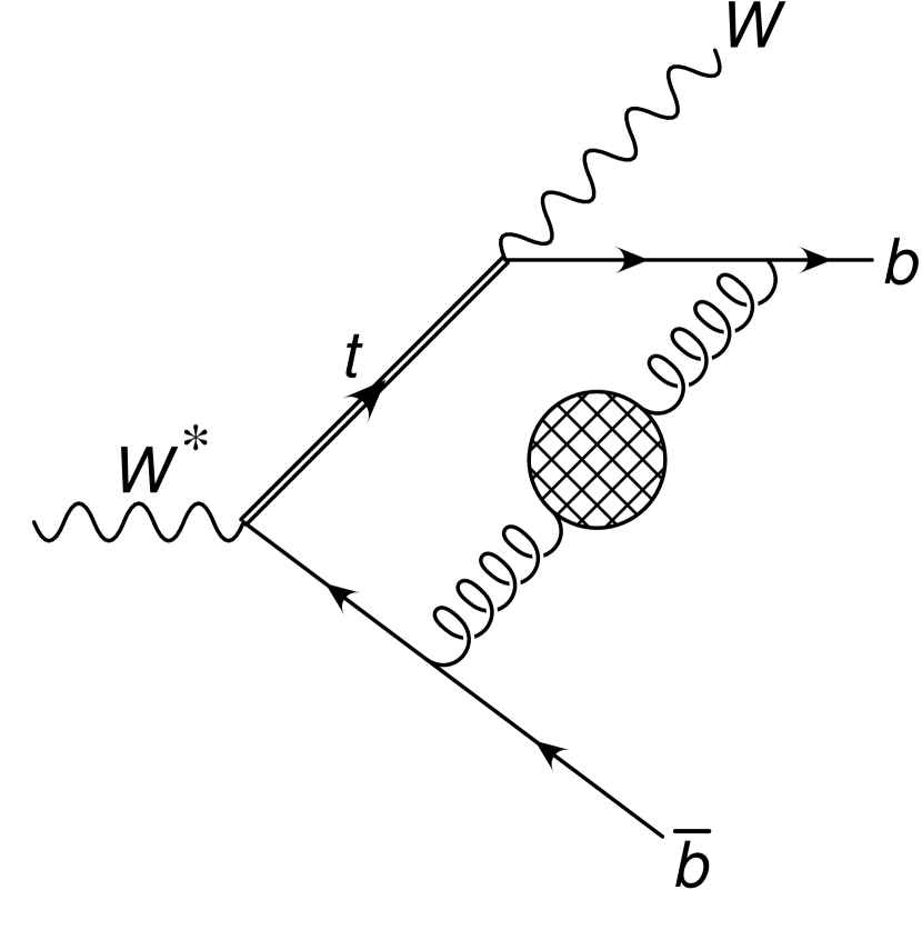
(b)

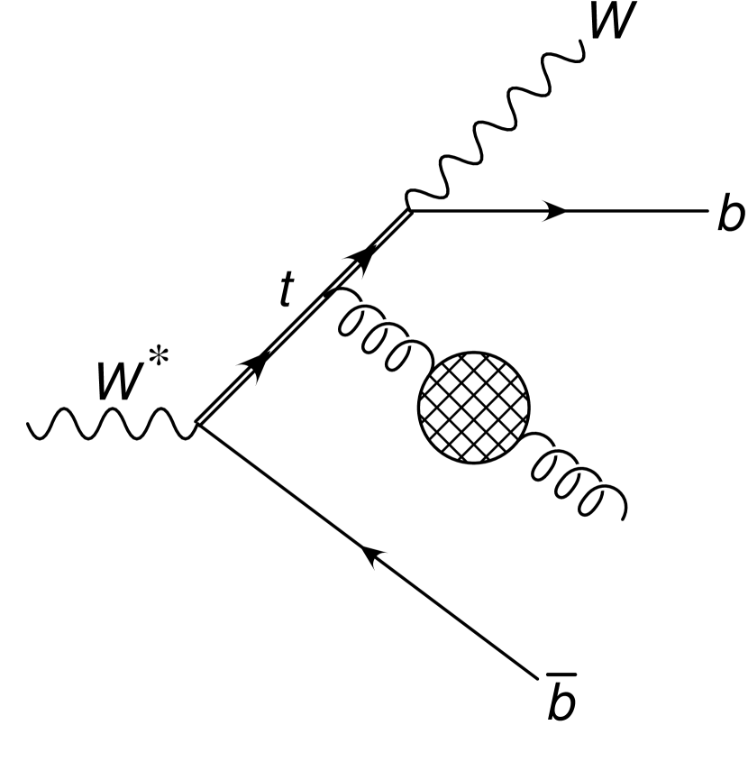
(c)

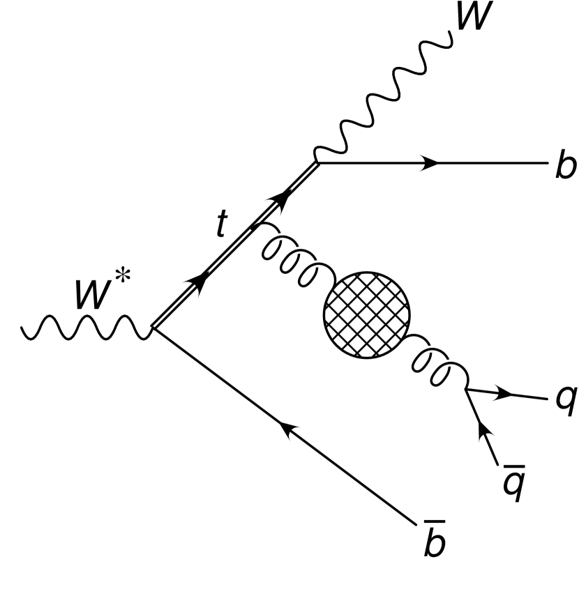
(d)

(e)

Figure 4.1: Feynman diagram for the Born $W^{*}\to Wb\bar{b}$ process (a), and samples of Feynman diagrams for the virtual contribution (b), for the real-emission contribution (c) and for $W^{*}\to Wb\bar{b}q\bar{q}$ production (d).

We now describe how we compute the total cross section. We use the complex pole scheme definition for the top mass. We assume the eventual presence of a set of cuts $\Theta(\Phi)$, function of the final state kinematics $\Phi$. The integrated cross section reads

$$\sigma = \int\mathrm{d}\Phi_{\operatorname{b}}\,\frac{\mathrm{d}\sigma_{\operatorname{b}}(\Phi_{\operatorname{b}})}{\mathrm{d}\Phi_{\operatorname{b}}}\,\Theta(\Phi_{\operatorname{b}})+\int\mathrm{d}\Phi_{\operatorname{b}}\,\frac{\mathrm{d}\sigma_{\operatorname{v}}(\Phi_{\operatorname{b}})}{\mathrm{d}\Phi_{\operatorname{b}}}\,\Theta(\Phi_{\operatorname{b}})+\int\mathrm{d}\Phi_{g}\,\frac{\mathrm{d}\sigma_{g}(\Phi_{g})}{\mathrm{d}\Phi_{g}}\,\Theta(\Phi_{g})$$ (4.7)

$$\hskip 19.91684pt+\int\mathrm{d}\Phi_{q\bar{q}}\,\frac{\mathrm{d}\sigma_{q\bar{q}}(\Phi_{q\bar{q}})}{\mathrm{d}\Phi_{q\bar{q}}}\,\Theta(\Phi_{q\bar{q}}),$$

where first term represents the Born contribution, the second the virtual one, the third term represents the contribution due to the emission of a real gluon and the fourth term represents the contribution with the real production of $n_{f}$ $q\bar{q}$ pairs. The last three contributions are potentially divergent. Equation (4.7) implicitly defines our notation for the different phase space integration volumes.

We always imply that the gluon propagators, in the last three contributions, include the sum of all vacuum polarization insertions of light quark loops.

We rewrite the total cross section as sum of four contributions:

$$\sigma = \sigma_{\operatorname{b}}+\sigma_{\operatorname{v}}+\sigma_{g^{*}}+\Delta\sigma_{q\bar{q}}\,,$$ (4.8)

$$\sigma_{\operatorname{b}} \equiv \int\mathrm{d}\Phi_{\operatorname{b}}\,\frac{\mathrm{d}\sigma_{\operatorname{b}}(\Phi_{\operatorname{b}})}{\mathrm{d}\Phi_{\operatorname{b}}}\,\Theta(\Phi_{\operatorname{b}})\,,$$ (4.9)

$$\sigma_{\operatorname{v}} \equiv \int\mathrm{d}\Phi_{\operatorname{b}}\,\frac{\mathrm{d}\sigma_{\operatorname{v}}(\Phi_{\operatorname{b}})}{\mathrm{d}\Phi_{\operatorname{b}}}\,\Theta(\Phi_{\operatorname{v}})\,,$$ (4.10)

$$\sigma_{g^{*}} \equiv \int\mathrm{d}\Phi_{g}\,\frac{\mathrm{d}\sigma_{g}(\Phi_{g})}{\mathrm{d}\Phi_{g}}\,\Theta(\Phi_{g})+\int\mathrm{d}\Phi_{q\bar{q}}\frac{\mathrm{d}\sigma_{q\bar{q}}(\Phi_{q\bar{q}})}{\mathrm{d}\Phi_{q\bar{q}}}\,\Theta(\Phi_{g^{*}})\,,$$ (4.11)

$$\Delta\sigma_{q\bar{q}} \equiv \int\mathrm{d}\Phi_{q\bar{q}}\,\frac{\mathrm{d}\sigma_{q\bar{q}}(\Phi_{q\bar{q}})}{\mathrm{d}\Phi_{q\bar{q}}}\left[\Theta(\Phi_{q\bar{q}})-\Theta(\Phi_{g^{*}})\right]\,,$$ (4.12)

where the selection cuts $\Theta(\Phi_{g^{*}})$ are evaluated with the same kinematics of the $Wb\bar{b}q\bar{q}$ events but with the $q\bar{q}$ pair clustered in a single jet ($g^{*}$).

4.1 The $\boldsymbol{\Delta\sigma_{q\bar{q}}}$ contribution

In this section we illustrate how to calculate the term $\Delta\sigma_{q\bar{q}}$ of eq. (4.8). $\Delta\sigma_{q\bar{q}}$ receives contributions only from the real graphs with a final state $Wb\bar{b}q\bar{q}$, where $q\bar{q}$ is a pair of light quarks, as depicted in Fig. 4.1 (d).

Starting from the ${\cal O}(\alpha_{\mathchoice{\displaystyle}{\scriptstyle}{\scriptscriptstyle}{\scriptscriptstyle}\rm S}^{2})$ tree-level cross section for the process $W^{*}\to Wb\bar{b}q\bar{q}$, that we indicate as $\mathrm{d}\sigma^{(2)}_{q\bar{q}}$, with no vacuum polarization insertions in the gluon propagator, we obtain the differential cross section $\mathrm{d}\sigma_{q\bar{q}}$ with the insertion of all the light-quark bubbles by simply replacing the bare gluon propagator with the dressed one of eq. (3.10)

$$\frac{\mathrm{d}\sigma_{q\bar{q}}(\Phi_{q\bar{q}})}{\mathrm{d}\Phi_{q\bar{q}}}=\frac{\mathrm{d}\sigma^{(2)}_{q\bar{q}}(\Phi_{q\bar{q}})}{\mathrm{d}\Phi_{q\bar{q}}}\left|\frac{1}{1+\Pi(k^{2},\mu^{2})-\Pi_{\operatorname{ct}}}\right|^{2},$$ (4.13)

where $k^{2}$ is the virtuality of the $q\bar{q}$ pair arising after the gluon splitting. In order to compute $\Delta\sigma_{q\bar{q}}$, we insert this equation into (4.12), and we get

$$\Delta\sigma_{q\bar{q}}=\int\mathrm{d}\lambda^{2}\,\delta(k^{2}-\lambda^{2})\,\int\mathrm{d}\Phi_{q\bar{q}}\,\frac{\mathrm{d}\sigma^{(2)}_{q\bar{q}}(\Phi_{q\bar{q}})}{\mathrm{d}\Phi_{q\bar{q}}}\,\Big{[}\Theta(\Phi_{q\bar{q}})-\Theta(\Phi_{g^{*}})\Big{]}\,\left|\frac{1}{1+\Pi(\lambda^{2},\mu^{2})-\Pi_{\operatorname{ct}}}\right|^{2},$$ (4.14)

where we have added the dummy integration $\int\mathrm{d}\lambda^{2}\,\delta(k^{2}-\lambda^{2})=1$. We remark that, thanks to the subtraction in the square parenthesis in eq. (4.14), $\Delta\sigma_{q\bar{q}}$ is finite as $\lambda^{2}\rightarrow 0$. In fact, if $\lambda^{2}\rightarrow 0$ in the collinear sense, the first clustering of the jet algorithm is the one of the $q\bar{q}$ pair into a $g^{*}$ (since $\Phi_{q\bar{q}}\rightarrow\Phi_{g^{*}}$), unless the gluon three-momentum just happens to lay on the jet cone. But, in this case, the direction of the pair must be closer to the cone than the pair aperture, and this leads to a suppression of the cross section of the order of the pair separation. The finiteness in the case of soft $\lambda$ is obvious, since the reconstructed mass is insensitive to soft particles. Notice that the integral is finite in the sense that the integrand goes like $1/\lambda$, and it is integrated in $\mathrm{d}\lambda^{2}$. For large $\lambda$, the integrand is zero for kinematic constraints, thus the integral is finite.

In order to make contact to other contributions we are going to compute, we write the absolute square of the dressed propagator in terms of the derivative of an imaginary part. We can perform the following manipulation

$$\left|\frac{1}{1+\Pi(\lambda^{2},\mu^{2})-\Pi_{\operatorname{ct}}}\right|^{2} = -\frac{1}{{\rm Im}\,\Pi(\lambda^{2},\mu^{2})}\,{\rm Im}\left[\frac{1}{1+\Pi(\lambda^{2},\mu^{2})-\Pi_{\operatorname{ct}}}\right]$$ (4.15)

$$= \frac{1}{\alpha_{\mathchoice{\displaystyle}{\scriptstyle}{\scriptscriptstyle}{\scriptscriptstyle}\rm S}\,\pi\,b_{0}}\,\operatorname{Im}\left[\frac{1}{1+\Pi(\lambda^{2},\mu^{2})-\Pi_{\operatorname{ct}}}\right]$$

$$= \frac{\lambda^{2}}{\alpha_{\mathchoice{\displaystyle}{\scriptstyle}{\scriptscriptstyle}{\scriptscriptstyle}\rm S}\,\pi\,b_{0}}\,{\rm Im}\left[\frac{1}{\lambda^{2}+i\eta}\frac{1}{1+\Pi(\lambda^{2},\mu^{2})-\Pi_{\operatorname{ct}}}\right].\qquad$$

since this factor multiplies an expression that is regular for $\lambda=0$, and thus the $\delta(\lambda)$ arising from the imaginary part (see eq. (B.9)) does not contribute. Using eq. (3.38) we are lead to

$$\left|\frac{1}{1+\Pi(\lambda^{2},\mu^{2})-\Pi_{\operatorname{ct}}}\right|^{2} = \frac{\lambda^{2}}{\alpha_{\mathchoice{\displaystyle}{\scriptstyle}{\scriptscriptstyle}{\scriptscriptstyle}\rm S}^{2}\,\pi\,b_{0,f}^{2}}\,\frac{\mathrm{d}\ }{\mathrm{d}\lambda^{2}}\,{\rm Im}\left\{\log\left[1+\Pi\left(\lambda^{2},\mu^{2}\right)-\Pi_{\operatorname{ct}}\right]\right\}$$ (4.16)

Equation (4.14) becomes

$$\Delta\sigma_{q\bar{q}} = \int\frac{\mathrm{d}\lambda^{2}}{\pi}\,\delta(k^{2}-\lambda^{2})\int\mathrm{d}\Phi_{q\bar{q}}\,\frac{\mathrm{d}\sigma^{(2)}_{q\bar{q}}(\Phi_{q\bar{q}})}{\mathrm{d}\Phi_{q\bar{q}}}\,\Big{[}\Theta(\Phi_{q\bar{q}})-\Theta(\Phi_{g^{*}})\Big{]}$$ (4.17)

$$\phantom{\int}\times\frac{\lambda^{2}}{\alpha_{\mathchoice{\displaystyle}{\scriptstyle}{\scriptscriptstyle}{\scriptscriptstyle}\rm S}^{2}\,b_{0,f}^{2}}\,\frac{\mathrm{d}}{\mathrm{d}\lambda^{2}}\,{\rm Im}\left\{\log\left[1+\Pi(\lambda^{2}+i\eta,\mu^{2})-\Pi_{\operatorname{ct}}\right]\right\}.$$

Defining

$$\Delta\!\left(\lambda\right)\equiv-\frac{\lambda^{2}}{\alpha_{\mathchoice{\displaystyle}{\scriptstyle}{\scriptscriptstyle}{\scriptscriptstyle}\rm S}\,b_{0,f}}\int\delta(k^{2}-\lambda^{2})\,\mathrm{d}\Phi_{q\bar{q}}\,\frac{\mathrm{d}\sigma^{(2)}_{q\bar{q}}(\Phi_{q\bar{q}})}{\mathrm{d}\Phi_{q\bar{q}}}\,\Big{[}\Theta(\Phi_{q\bar{q}})-\Theta(\Phi_{g^{*}})\Big{]},$$ (4.18)

and integrating by parts eq. (4.17), we are lead to

$$\Delta\sigma_{q\bar{q}}=\frac{1}{\alpha_{\mathchoice{\displaystyle}{\scriptstyle}{\scriptscriptstyle}{\scriptscriptstyle}\rm S}\,b_{0,f}}\int_{0}\frac{\mathrm{d}\lambda}{\pi}\,\frac{\mathrm{d}\ }{\mathrm{d}\lambda}\!\left[\Delta\!\left(\lambda\right)\right]\,{\rm Im}\left\{\log\left[1+\Pi(\lambda^{2}+i\eta,\mu^{2})-\Pi_{\operatorname{ct}}\right]\right\},$$ (4.19)

where the integrand function is identically 0 for $\lambda\geq\sqrt{s}-m_{\mathchoice{\displaystyle}{\scriptstyle}{\scriptscriptstyle}{\scriptscriptstyle}W}$. We remind the reader that the cross section $\sigma^{(2)}_{q\bar{q}}$ and $b_{0,f}$ are both proportional to $n_{f}$, that thus cancels in the definition of $\Delta(\lambda)$, so when we will move from the large-$n_{f}$ to the large-$b_{0}$ limit, $\Delta(\lambda)$ will not change.

4.2 The $\boldsymbol{\sigma_{g^{*}}}$ contribution

The ${\sigma_{g^{*}}}$ term of eq. (4.11) receives contributions from final states with both a single real gluon or a $q\bar{q}$ pair. Both these contributions have collinear divergences related to the $q\bar{q}$ splitting that cancel when integrating the latter over $\lambda^{2}$ and summing them up.

4.2.1 The gluon contribution

The first contribution of eq. (4.11) can be computed starting from $\sigma_{g}^{(1)}$, the tree-level cross section for the emission of a single gluon. The sum over all the polarization insertions gives rise to the the following identity

$$\int\mathrm{d}\Phi_{g}\,\frac{\mathrm{d}\sigma_{g}(\Phi_{g})}{\mathrm{d}\Phi_{g}}\,{O}(\Phi_{g})=\int\mathrm{d}\Phi_{g}\,\frac{\mathrm{d}\sigma_{g}^{(1)}(\Phi_{g})}{\mathrm{d}\Phi_{g}}\,{O}(\Phi_{g})\,\frac{1}{1+\Pi(0,\mu^{2})-\Pi_{\operatorname{ct}}}.$$ (4.20)

Since $\Pi(0,\mu^{2})$ is not well-defined, it is convenient to assign to the quarks in the polarization bubbles a small mass $m_{q}$. We indicate the self-energy correction with a massive quark with $\Pi(0,m_{q}^{2},\mu^{2})$. Indeed it can be easily shown that

$$\Pi(0,m_{q}^{2},\mu^{2})=\frac{\alpha_{\mathchoice{\displaystyle}{\scriptstyle}{\scriptscriptstyle}{\scriptscriptstyle}\rm S}T_{\mathchoice{\displaystyle}{\scriptstyle}{\scriptscriptstyle}{\scriptscriptstyle}\rm F}}{3\pi}\left[\frac{1}{\epsilon}-\log\left(\frac{m_{q}^{2}}{\mu^{2}}\right)\right]+{\cal O}(\epsilon)\,,$$ (4.21)

that is well defined and real. The analytic expression of $\Pi(k^{2},m_{q}^{2},\mu^{2})-\Pi_{\rm ct}$ for an arbitrary $k^{2}$ value is given in eq. (3.14). We can then write

$$\int\mathrm{d}\Phi_{g}\,\frac{\mathrm{d}\sigma_{g}(\Phi_{g})}{\mathrm{d}\Phi_{g}}\,\Theta(\Phi_{g})=\int\mathrm{d}\Phi_{g}\,\frac{\mathrm{d}\sigma_{g}^{(1)}(\Phi_{g})}{\mathrm{d}\Phi_{g}}\,{O}(\Phi_{g})\,\frac{1}{1+\Pi(0,m_{q}^{2},\mu^{2})-\Pi_{\operatorname{ct}}}.$$ (4.22)

4.2.2 The $\boldsymbol{q\bar{q}}$ contribution

In order to treat the second term of eq. (4.11), we first discuss the relation between $\sigma^{(2)}_{q\bar{q}}$, the cross section for the production of $n_{f}$ $q\bar{q}$ pairs with invariant mass $\lambda$, and $\sigma^{(1)}_{g^{*}}$, the cross section for the production of a massive gluon whose four-momentum $k^{\mu}$ is equal to the sum of the $q$ and $\bar{q}$ momenta. We have

$$\frac{\mathrm{d}\sigma^{(1)}_{g^{*}}(\lambda,\Phi_{g^{*}})}{\mathrm{d}\Phi_{g^{*}}} = \frac{1}{2s}\mathcal{M}_{g^{*}}^{\mu}(\Phi_{g^{*}})\mathcal{M}_{g^{*}}^{\nu*}(\Phi_{g^{*}})\sum_{\rm pol}\epsilon_{\mu}\left(\lambda\right)\epsilon^{*}_{\nu}\left(\lambda\right)$$ (4.23)

$$= \frac{1}{2s}\mathcal{M}_{g^{*}}^{\mu}(\Phi_{g^{*}})\mathcal{M}_{g^{*}}^{\nu*}(\Phi_{g^{*}})\left[-g_{\mu\nu}+\frac{k_{\mu}k_{\nu}}{\lambda^{2}}\right]$$

where $1/2s$ is the flux factor and $\mathcal{M}_{g^{*}}^{\mu}(\Phi_{g^{*}})$ is the amplitude for the production of a massive gluon $g^{*}$ of momentum $k^{\mu}$, not contracted with its polarization vector $\epsilon^{\mu}(k)$. The real phase space $\Phi_{q\bar{q}}$ can be written as the product of the phase space for the production of a gluon with virtuality $k^{2}$, that we call $\mathrm{d}\Phi_{g^{*}}$, and its decay into a $q\bar{q}$ pair, $\mathrm{d}\Phi_{\operatorname{dec}}$

$$\mathrm{d}\Phi_{q\bar{q}}=\frac{\mathrm{d}k^{2}}{2\pi}\,\mathrm{d}\Phi_{g^{*}}\,\mathrm{d}\Phi_{\operatorname{dec}}\,.$$ (4.24)

Applying the optical theorem we have

$$\int_{4m_{q}^{2}}\mathrm{d}k^{2}\int\mathrm{d}\Phi_{\operatorname{dec}} \,\frac{\mathrm{d}\sigma^{(2)}_{q\bar{q}}(\Phi_{q\bar{q}})}{\mathrm{d}\Phi_{q\bar{q}}}\,\delta(k^{2}-\lambda^{2})$$

$$=2\left[\frac{\mathcal{M}_{g^{*}}^{\mu}(\Phi_{g^{*}})\mathcal{M}_{g^{*}}^{\nu,*}(\Phi_{g^{*}})}{2s}\frac{1}{\lambda^{4}}\,{\rm Im}\,\Pi(\lambda^{2},m_{q}^{2},\mu^{2})\left(-\lambda^{2}\,g_{\mu\nu}+k_{\mu}k_{\nu}\right)\right]$$

$$=\frac{\mathrm{d}\sigma^{(1)}_{g^{*}}(\lambda,\Phi_{g^{*}})}{\mathrm{d}\Phi_{g^{*}}}\frac{2\,{\rm Im}\left[\Pi(\lambda^{2},m_{q}^{2},\mu^{2})\right]}{\lambda^{2}},$$ (4.25)

where the imaginary part vanishes for $k^{2}\leq 4m_{q}^{2}$. Using eqs. (4.14) and (4.25) enables us to rewrite the $q\bar{q}$ splitting term as

$$\int\mathrm{d}\Phi_{q\bar{q}}\,\frac{\mathrm{d}\sigma_{q\bar{q}}(\Phi_{q\bar{q}})}{\mathrm{d}\Phi_{q\bar{q}}}\,\Theta(\Phi_{g^{*}})=\int_{4m_{q}^{2}}\mathrm{d}\lambda^{2}\,\delta(k^{2}-\lambda^{2})\int\mathrm{d}\Phi_{q\bar{q}}\,\frac{\mathrm{d}\sigma_{q\bar{q}}(\Phi_{q\bar{q}})}{\mathrm{d}\Phi_{q\bar{q}}}\,\Theta(\Phi_{g^{*}})$$

$$\hskip 14.22636pt=\int_{4m_{q}^{2}}\frac{\mathrm{d}\lambda^{2}}{2\pi}\int\mathrm{d}\Phi_{g^{*}}\int\mathrm{d}\Phi_{\rm dec}\,\frac{\mathrm{d}\sigma^{(2)}_{q\bar{q}}(\Phi_{q\bar{q}})}{\mathrm{d}\Phi_{q\bar{q}}}\frac{1}{\left|1+\Pi(\lambda^{2}+i\eta,m_{q}^{2},\mu^{2})-\Pi_{\operatorname{ct}}\right|^{2}}\,\Theta(\Phi_{g^{*}})$$

$$\hskip 14.22636pt=\frac{1}{\pi}\int_{4m_{q}^{2}}\frac{\mathrm{d}\lambda^{2}}{\lambda^{2}}\int\mathrm{d}\Phi_{g^{*}}\,\frac{\mathrm{d}\sigma_{g^{*}}^{(1)}(\lambda,\Phi_{g^{*}})}{\mathrm{d}\Phi_{g^{*}}}\,\frac{{\rm Im}\,\Pi(\lambda^{2},m_{q}^{2},\mu^{2})}{\left|1+\Pi(\lambda^{2}+i\eta,m_{q}^{2},\mu^{2})-\Pi_{\operatorname{ct}}\right|^{2}}\,\Theta(\Phi_{g^{*}})\,.\phantom{aaaaaaa}$$ (4.26)

4.2.3 Combination of the gluon and $\boldsymbol{q\bar{q}}$ contributions

Defining

$$R(\lambda)=\int\mathrm{d}\Phi_{g^{*}}\,\frac{\sigma_{g^{*}}^{(1)}(\lambda,\Phi_{g^{*}})}{\mathrm{d}\Phi_{g^{*}}}\Theta(\Phi_{g^{*}}),$$ (4.27)

we can combine eq. (4.22) and (4.2.2) and get

$$\sigma_{g^{*}}=R^{(\epsilon)}(0)\frac{1}{1+\Pi(0,m_{q}^{2},\mu^{2})-\Pi_{\rm ct}}-\frac{1}{\pi}\int_{4m_{q}^{2}}\frac{\mathrm{d}\lambda^{2}}{\lambda^{2}}R(\lambda)\,{\rm Im}\frac{1}{1+\Pi(\lambda^{2},m_{q}^{2},\mu^{2})-\Pi_{\rm ct}}\,.$$ (4.28)

With the notation $R^{(\epsilon)}(0)$ we remind the reader that for $\lambda=0$ there are infrared divergences in $R$ that are regulated in dimensional regularization.

4.3 The $\boldsymbol{\sigma_{\rm v}}$ contribution

The NLO differential virtual cross-section can be represented as

$$\frac{\mathrm{d}\sigma^{(1)}_{\rm v}(\Phi_{\rm b})}{\mathrm{d}\Phi_{\rm b}}=\int\frac{\mathrm{d}^{d}k}{(2\pi)^{d}}\frac{F_{\rm virt}(k,\Phi_{\rm b})}{k^{2}+i\eta}\,,$$ (4.29)

where $k^{2}$ is the loop momentum and $d=4-2\epsilon$. By replacing the free gluon propagator with the dressed one, we obtain the all-orders expression $\sigma_{\rm v}(\Phi_{\rm b})$

$$\frac{\mathrm{d}\sigma_{\rm v}(\Phi_{\rm b})}{\mathrm{d}\Phi_{\rm b}}=\int\frac{\mathrm{d}^{d}k}{(2\pi)^{d}}\frac{F_{\rm virt}(k,\Phi_{\rm b})}{k^{2}+i\eta}\frac{1}{1+\Pi(k^{2},\mu^{2})-\Pi_{\rm ct}}\,.$$ (4.30)

If we use eq. (B.8), we obtain

$$\frac{\mathrm{d}\sigma_{\rm v}(\Phi_{\rm b})}{\mathrm{d}\Phi_{\rm b}} = -\frac{1}{\pi}\int_{4m_{q}^{2}}^{+\infty}\frac{\mathrm{d}\lambda^{2}}{\lambda^{2}}\int\frac{\mathrm{d}^{d}k}{(2\pi)^{d}}\frac{F_{\rm virt}(k,\Phi_{\rm b})}{k^{2}-\lambda^{2}+i\eta}\,{\rm Im}\left\{\frac{1}{\Pi(\lambda^{2},m_{q}^{2},\mu^{2})-\Pi_{\rm ct}}\right\}\!\!$$ (4.31)

$$+\int\frac{\mathrm{d}^{d}k}{(2\pi)^{d}}\frac{F_{\rm virt}(k,\Phi_{\rm b})}{k^{2}+i\eta}\frac{1}{\Pi(0,m_{q}^{2},\mu^{2})-\Pi_{\rm ct}},$$

where $m_{q}$ is the light quark mass that has been introduced to regulate the bad behaviour of $\Pi(0,\mu^{2})$. We define

$$V(\lambda)\equiv\int\mathrm{d}\Phi_{\rm b}\Theta(\Phi_{\rm b})\int\frac{\mathrm{d}^{d}k}{(2\pi)^{d}}\frac{F_{\rm virt}(k,\Phi_{\rm b})}{k^{2}-\lambda^{2}+i\eta}=\int\mathrm{d}\Phi_{\rm b}\Theta(\Phi_{\rm b})\,\frac{\mathrm{d}\sigma^{(1)}_{\rm v}\left(\lambda,\Phi_{\rm b}\right)}{\mathrm{d}\Phi_{\rm b}}\,,$$ (4.32)

where $\mathrm{d}\sigma^{(1)}_{\rm v}(\lambda,\Phi_{\rm b})$ is the differential virtual cross section computed with a gluon of mass $\lambda$. The ${\sigma_{\rm v}}$ of eq. (4.10) can be finally rewritten as

$$\sigma_{\rm v}=V^{(\epsilon)}(0)\frac{1}{1+\Pi(0,m_{q}^{2},\mu^{2})-\Pi_{\rm ct}}\,-\,\frac{1}{\pi}\int\frac{\mathrm{d}\lambda^{2}}{\lambda^{2}}V(\lambda)\,{\rm Im}\frac{1}{1+\Pi(\lambda^{2},m_{q}^{2},\mu^{2})-\Pi_{\rm ct}}\,,$$ (4.33)

where the notation $V^{(\epsilon)}(0)$ signals the presence of the leftover IR divergences for $\lambda=0$, that are handled in dimensional regularization. If a finite gluon mass $\lambda$ is employed, IR singularities are regulated by single and double logarithms of $\lambda$. If we choose the pole mass scheme, $V(\lambda)\to\frac{1}{\lambda^{2}}$ for large $\lambda$. Furthermore, $V(\lambda)/\alpha_{\mathchoice{\displaystyle}{\scriptstyle}{\scriptscriptstyle}{\scriptscriptstyle}\rm S}$ does not depend on $\mu$. This signals that there are no UV divergences. Thus $V(\lambda)$, with $\lambda>0$, can be evaluated performing the $\epsilon\to 0$ limit since the integral in eq. (4.33) is finite.

4.4 Combining the virtual and the real contributions

We define

$$S(\lambda)\equiv R(\lambda)+V(\lambda)\,,$$ (4.34)

with $R$ and $V$ given by eqs. (4.27) and (4.32) respectively. As long as $\lambda$ is not zero, $R$ and $V$ are separately well defined in $d=4$ dimensions, but they are IR divergent for $\lambda\to 0$. However, as required by the KLN theorem, their sum $S$ is finite in that limit, indeed

$$S(0)=\lim_{\lambda\to 0}\Big{[}R(\lambda)+V(\lambda)\Big{]}=\lim_{\epsilon\to 0}\left[R^{(\epsilon)}(0)+V^{(\epsilon)}(0)\right]=\sigma^{(1)},$$ (4.35)

being $\sigma^{(1)}$ the integrated NLO cross section. Thus, summing eqs. (4.33) and (4.28), we have

$$\sigma_{\rm v}+\sigma_{g^{*}} = S(0)\frac{1}{1+\Pi(0,m_{q}^{2},\mu^{2})-\Pi_{\operatorname{ct}}}$$ (4.36)

$$-\frac{1}{\pi}\int_{4m_{q}^{2}}^{+\infty}\frac{\mathrm{d}\lambda^{2}}{\lambda^{2}}\,S(\lambda)\,{\rm Im}\left[\frac{1}{1+\Pi(\lambda^{2},m_{q}^{2},\mu^{2})-\Pi_{\operatorname{ct}}}\right]$$

$$= -\int_{0^{-}}^{+\infty}\frac{\mathrm{d}\lambda^{2}}{\pi}\,S(\lambda)\,{\rm Im}\left[\frac{1}{\lambda^{2}+i\eta}\,\frac{1}{1+\Pi(\lambda^{2},m_{q}^{2},\mu^{2})-\Pi_{\operatorname{ct}}}\right],\phantom{aaaa}$$

where in the last line we have used eq. (B.9) and the fact that the limit $\lambda\to 0$ is well defined for $S$, while this was not the case for $V$ and $R$ separately. We can check that at $\mathcal{O}(\alpha_{\mathchoice{\displaystyle}{\scriptstyle}{\scriptscriptstyle}{\scriptscriptstyle}\rm S})$ we recover the NLO result

$$\left[\sigma_{\rm v}+\sigma_{g^{*}}\right]_{\mathcal{O}(\alpha_{\mathchoice{\displaystyle}{\scriptstyle}{\scriptscriptstyle}{\scriptscriptstyle}\rm S})}=-\int_{0^{-}}^{+\infty}\frac{\mathrm{d}\lambda^{2}}{\pi}\,S(\lambda)\,{\rm Im}\left[\frac{1}{\lambda^{2}+i\eta}\,\right]=-\int\frac{\mathrm{d}\lambda^{2}}{\pi}\,S(\lambda)\left[-\pi\,\delta(\lambda^{2})\right]=\sigma^{(1)}\,.$$ (4.37)

We now illustrate a procedure to safety take the limit $m_{q}\to 0$ in eq. (4.36). We can write eq. (4.36) by adding and subtracting the same term

$$\sigma_{g}+\sigma_{\operatorname{v}}= -\int_{0^{-}}^{\infty}\frac{\mathrm{d}\lambda^{2}}{\pi}\left[S(\lambda)-S(0)\,\frac{\mu^{2}}{\lambda^{2}+\mu^{2}}\right]{\rm Im}\left[\frac{1}{\lambda^{2}+i\eta}\,\frac{1}{1+\Pi(\lambda^{2},m_{q}^{2},\mu^{2})-\Pi_{\operatorname{ct}}}\right]$$

$$-\int_{0^{-}}^{\infty}\frac{\mathrm{d}\lambda^{2}}{\pi}S(0)\,\frac{\mu^{2}}{\lambda^{2}+\mu^{2}}\,{\rm Im}\left[\frac{1}{\lambda^{2}+i\eta}\frac{1}{1+\Pi(\lambda^{2},m_{q}^{2},\mu^{2})-\Pi_{\operatorname{ct}}}\right],$$ (4.38)

where $\mu^{2}$ is a real positive number. The first integral is regular for $\lambda^{2}\rightarrow 0$ also if $m_{q}=0$, since the term in the square brackets is ${\cal O}(\lambda)$ in this limit. This also enables us to move the lower bound from $0^{-}$ to $0$. Using the identity already employed in eq. (3.38), we are left to

$$\int_{0}^{\infty}\frac{\mathrm{d}\lambda^{2}}{\pi}\left[S(\lambda)-S(0)\,\frac{\mu^{2}}{\lambda^{2}+\mu^{2}}\right]{\rm Im}\left[\frac{1}{\lambda^{2}+i\eta}\,\frac{1}{1+\Pi(\lambda^{2},\mu^{2})-\Pi_{\operatorname{ct}}}\right]$$

$$\hskip 5.69046pt=\int_{0}^{\infty}\frac{\mathrm{d}\lambda^{2}}{\pi}\left[S(\lambda)-S(0)\,\frac{\mu^{2}}{\lambda^{2}+\mu^{2}}\right]{\rm Im}\left\{\frac{1}{\alpha_{\mathchoice{\displaystyle}{\scriptstyle}{\scriptscriptstyle}{\scriptscriptstyle}\rm S}\,b_{0,f}}\,\frac{\mathrm{d}\ }{\mathrm{d}\lambda^{2}}\log\left[1+\Pi\left(\lambda^{2},\mu^{2}\right)-\Pi_{\operatorname{ct}}\right]\right\}$$

$$\hskip 5.69046pt=-\int_{0}^{\infty}\frac{\mathrm{d}\lambda^{2}}{\pi}\frac{\mathrm{d}\ }{\mathrm{d}\lambda^{2}}\left[S(\lambda)-S(0)\,\frac{\mu^{2}}{\lambda^{2}+\mu^{2}}\right]\frac{1}{\alpha_{\mathchoice{\displaystyle}{\scriptstyle}{\scriptscriptstyle}{\scriptscriptstyle}\rm S}\,b_{0,f}}\,{\rm Im}\left\{\log\left[1+\Pi\left(\lambda^{2},\mu^{2}\right)-\Pi_{\operatorname{ct}}\right]\right\},$$

where the boundary terms vanish, since $S(\lambda)$ vanishes for large $\lambda$ (if the pole scheme is adopted), and the difference in the square brackets is zero for $\lambda=0$.

The second integral can be extended below from $0^{-}$ to $-\mu^{2}/2$, since the imaginary part is zero for $\lambda^{2}<0$. We can rewrite

$$\int_{0^{-}}^{\infty}\frac{\mathrm{d}\lambda^{2}}{\pi}S(0)\,\frac{\mu^{2}}{\lambda^{2}+\mu^{2}}\,{\rm Im}\left[\frac{1}{\lambda^{2}+i\eta}\,\frac{1}{1+\Pi(\lambda^{2},m_{q}^{2},\mu^{2})-\Pi_{\operatorname{ct}}}\right]$$

$${}\hskip 14.22636pt=\int_{-\mu^{2}/2}^{\infty}\frac{\mathrm{d}\lambda^{2}}{\pi}S(0)\,\frac{\mu^{2}}{\lambda^{2}+\mu^{2}}\,{\rm Im}\left[\frac{1}{\lambda^{2}+i\eta}\,\frac{1}{1+\Pi(\lambda^{2},m_{q}^{2},\mu^{2})-\Pi_{\operatorname{ct}}}\right]$$

$${}\hskip 14.22636pt=\frac{1}{2i}\oint\frac{\mathrm{d}\lambda^{2}}{\pi}S(0)\,\frac{\mu^{2}}{\lambda^{2}+\mu^{2}}\,\frac{1}{\lambda^{2}}\,\frac{1}{1+\Pi(\lambda^{2},m_{q}^{2},\mu^{2})-\Pi_{\operatorname{ct}}}\,,$$ (4.40)

where the contour is depicted in Fig. 4.2.

Figure 4.2: Integration path.

The integral in the last line is equal to the residue at $\lambda^{2}=-\mu^{2}$, that is well-defined also for $m_{q}=0$. This allows us to safely take the limit $m_{q}\rightarrow 0$. By using eq. (3.38), and integrating by parts, we are lead to

$$\frac{1}{2i}\oint\frac{\mathrm{d}\lambda^{2}}{\pi}S(0)\,\frac{m^{2}}{\lambda^{2}+m^{2}}\,\frac{1}{\lambda^{2}}\,\frac{1}{1+\Pi(\lambda^{2},\mu^{2})-\Pi_{\operatorname{ct}}}$$

$$\hskip 14.22636pt=\frac{1}{2i}\oint\frac{\mathrm{d}\lambda^{2}}{\pi}S(0)\,\frac{m^{2}}{\lambda^{2}+m^{2}}\,\frac{1}{\alpha_{\mathchoice{\displaystyle}{\scriptstyle}{\scriptscriptstyle}{\scriptscriptstyle}\rm S}\,b_{0,f}}\,\frac{\mathrm{d}\ }{\mathrm{d}\lambda^{2}}\log\left[1+\Pi\left(\lambda^{2},\mu^{2}\right)-\Pi_{\operatorname{ct}}\right]$$

$$\hskip 14.22636pt=-\frac{1}{2i}\oint\frac{\mathrm{d}\lambda^{2}}{\pi}S(0)\,\frac{\mathrm{d}\ }{\mathrm{d}\lambda^{2}}\left[\frac{\mu^{2}}{\lambda^{2}+\mu^{2}}\right]\frac{1}{\alpha_{\mathchoice{\displaystyle}{\scriptstyle}{\scriptscriptstyle}{\scriptscriptstyle}\rm S}\,b_{0,f}}\,\log\left[1+\Pi\left(\lambda^{2},\mu^{2}\right)-\Pi_{\operatorname{ct}})\right].\qquad$$ (4.41)

If we set to infinity the larger radius of the boundary in Fig. 4.2, its contribution vanishes. The same holds if the radius around $\lambda^{2}=-m^{2}/2$ becomes infinitesimal. We are thus left with

$$-\frac{1}{2i}\int_{-\mu^{2}/2}^{\infty}\frac{\mathrm{d}\lambda^{2}}{\pi}S(0)\,\frac{\mathrm{d}\ }{\mathrm{d}\lambda^{2}}\left[\frac{\mu^{2}}{\lambda^{2}+\mu^{2}}\right]\frac{1}{\alpha_{\mathchoice{\displaystyle}{\scriptstyle}{\scriptscriptstyle}{\scriptscriptstyle}\rm S}\,b_{0,f}}$$

$$\hskip 42.67912pt\times\Big{\{}\log\left[1+\Pi\left(\lambda^{2}+i\eta,\mu^{2}\right)-\Pi_{\operatorname{ct}}\right]-\log\left[1+\Pi\left(\lambda^{2}-i\eta,\mu^{2}\right)-\Pi_{\operatorname{ct}}\right]\Big{\}}$$

$$\hskip 14.22636pt=-\int_{-\mu^{2}/2}^{\infty}\frac{\mathrm{d}\lambda^{2}}{\pi}S(0)\,\frac{\mathrm{d}\ }{\mathrm{d}\lambda^{2}}\left[\frac{\mu^{2}}{\lambda^{2}+\mu^{2}}\right]\frac{1}{\alpha_{\mathchoice{\displaystyle}{\scriptstyle}{\scriptscriptstyle}{\scriptscriptstyle}\rm S}\,b_{0,f}}\,{\rm Im}\left\{\log\left[1+\Pi\left(\lambda^{2},\mu^{2}\right)-\Pi_{\operatorname{ct}}\right]\right\}$$

$$\hskip 14.22636pt=-\int_{0}^{\infty}\frac{\mathrm{d}\lambda^{2}}{\pi}S(0)\,\frac{\mathrm{d}\ }{\mathrm{d}\lambda^{2}}\left[\frac{\mu^{2}}{\lambda^{2}+\mu^{2}}\right]\frac{1}{\alpha_{\mathchoice{\displaystyle}{\scriptstyle}{\scriptscriptstyle}{\scriptscriptstyle}\rm S}\,b_{0,f}}\,{\rm Im}\left\{\log\left[1+\Pi\left(\lambda^{2},\mu^{2}\right)-\Pi_{\operatorname{ct}}\right]\right\},\phantom{aaaaaa}$$ (4.42)

where in the last step we used the fact that the the imaginary part vanishes for negative values of $\lambda$. Using the results of eqs. (4.4) and (4.42), we can write eq. (4.4) as

$$\sigma_{g}+\sigma_{\operatorname{v}}=\frac{1}{\alpha_{\mathchoice{\displaystyle}{\scriptstyle}{\scriptscriptstyle}{\scriptscriptstyle}\rm S}\,b_{0,f}}\int_{0}^{\infty}\frac{\mathrm{d}\lambda}{\pi}\,\frac{\mathrm{d}\ }{\mathrm{d}\lambda}\!\left[S(\lambda)\right]{\rm Im}\left\{\log\left[1+\Pi\left(\lambda^{2}+i\eta,\mu^{2}\right)-\Pi_{\operatorname{ct}}\right]\right\}.$$ (4.43)

4.5 Calculation summary

Here we summarize our findings. If we combine eqs. (4.43) and (4.19), we have

$$\!\!\!\!\!\!\!\!\!\sigma = \int\mathrm{d}\Phi_{\operatorname{b}}\,\frac{\mathrm{d}\sigma_{\operatorname{b}}(\Phi_{\operatorname{b}})}{\mathrm{d}\Phi_{\operatorname{b}}}\,\Theta(\Phi_{\operatorname{b}})+\int\mathrm{d}\Phi_{\operatorname{b}}\,\frac{\mathrm{d}\sigma_{\operatorname{v}}(\Phi_{\operatorname{b}})}{\mathrm{d}\Phi_{\operatorname{b}}}\,\Theta(\Phi_{\operatorname{b}})+\int\mathrm{d}\Phi_{g}\,\frac{\mathrm{d}\sigma_{g}(\Phi_{g})}{\mathrm{d}\Phi_{g}}\,\Theta(\Phi_{g})$$

$$+\int\mathrm{d}\Phi_{q\bar{q}}\,\frac{\mathrm{d}\sigma_{q\bar{q}}(\Phi_{q\bar{q}})}{\mathrm{d}\Phi_{q\bar{q}}}\,\Theta(\Phi_{q\bar{q}})$$

$$= \sigma_{\rm b}+\frac{1}{\alpha_{\mathchoice{\displaystyle}{\scriptstyle}{\scriptscriptstyle}{\scriptscriptstyle}\rm S}\,b_{0,f}}\int_{0}^{\infty}\frac{\mathrm{d}k}{\pi}\,\frac{\mathrm{d}\ }{\mathrm{d}k}\!\left[T(\lambda)\right]\,{\rm Im}\left\{\log\left[1+\Pi\left(\lambda^{2},\mu^{2}\right)-\Pi_{\operatorname{ct}}\right]\right\}\!$$

$$= \sigma_{\rm b}-\frac{1}{\alpha_{\mathchoice{\displaystyle}{\scriptstyle}{\scriptscriptstyle}{\scriptscriptstyle}\rm S}\,b_{0,f}}\int_{0}^{\infty}\frac{\mathrm{d}\lambda}{\pi}\,\frac{\mathrm{d}\ }{\mathrm{d}\lambda}\!\left[T(\lambda)\right]\,\arctan\left[\frac{\alpha_{\mathchoice{\displaystyle}{\scriptstyle}{\scriptscriptstyle}{\scriptscriptstyle}\rm S}\,\pi\,b_{0,f}}{1+\alpha_{\mathchoice{\displaystyle}{\scriptstyle}{\scriptscriptstyle}{\scriptscriptstyle}\rm S}\,b_{0,f}\log\left(\frac{\lambda^{2}}{\mu^{2}e^{C}}\right)}\right],$$ (4.45)

with

$$\sigma_{\operatorname{b}} = \int\mathrm{d}\Phi_{\operatorname{b}}\,\frac{\mathrm{d}\sigma_{\operatorname{b}}(\Phi_{\operatorname{b}})}{\mathrm{d}\Phi_{\operatorname{b}}}\,\Theta(\Phi_{\operatorname{b}})\,,$$ (4.46)

$$T(\lambda) = V(\lambda)+R(\lambda)+\Delta(\lambda)\,,$$ (4.47)

$$V(\lambda) = \int\mathrm{d}\Phi_{\rm b}\,\frac{\mathrm{d}\sigma^{(1)}_{\rm v}\left(\lambda,\Phi_{\rm b}\right)}{\mathrm{d}\Phi_{\rm b}}\Theta(\Phi_{\rm b})\,,$$ (4.48)

$$R(\lambda) = \int\mathrm{d}\Phi_{g^{*}}\,\frac{\mathrm{d}\sigma^{(1)}_{g^{*}}\left(\lambda,\Phi_{g^{*}}\right)}{\mathrm{d}\Phi_{g^{*}}}\,\Theta(\Phi_{g^{*}})\,,$$ (4.49)

$$\Delta\!\left(\lambda\right) = -\frac{\lambda^{2}}{\alpha_{\mathchoice{\displaystyle}{\scriptstyle}{\scriptscriptstyle}{\scriptscriptstyle}\rm S}\,b_{0,f}}\int\delta(k^{2}-\lambda^{2})\,\mathrm{d}\Phi_{q\bar{q}}\,\frac{\mathrm{d}\sigma^{(2)}_{q\bar{q}}(\Phi_{q\bar{q}})}{\mathrm{d}\Phi_{q\bar{q}}}\,\Big{[}\Theta(\Phi_{q\bar{q}})-\Theta(\Phi_{g^{*}})\Big{]}.$$ (4.50)

To obtain the final expression in eq. (4.45) we have employed the following identity

$${\rm Im}\left\{\log\left[1+\Pi\left(\lambda^{2},\mu^{2}\right)-\Pi_{\operatorname{ct}}\right]\right\}=-\arctan\left[\frac{\alpha_{\mathchoice{\displaystyle}{\scriptstyle}{\scriptscriptstyle}{\scriptscriptstyle}\rm S}\,\pi\,b_{0,f}}{1+\alpha_{\mathchoice{\displaystyle}{\scriptstyle}{\scriptscriptstyle}{\scriptscriptstyle}\rm S}\,b_{0,f}\log\left(\frac{\lambda^{2}}{\mu^{2}e^{C}}\right)}\right],$$ (4.51)

where in the right-hand side we have neglected the contribution

$$-\pi\Theta\left(\mu^{2}\exp\left(-\frac{1}{b_{0}\alpha_{\mathchoice{\displaystyle}{\scriptstyle}{\scriptscriptstyle}{\scriptscriptstyle}\rm S}}+C\right)-\lambda^{2}\right).$$ (4.52)

We stress that the perturbative expansion in $\alpha_{\mathchoice{\displaystyle}{\scriptstyle}{\scriptscriptstyle}{\scriptscriptstyle}\rm S}$ of formula (4.45) is an asymptotic one, and only its coefficients are unambiguously defined, and are the subject of the present work. Thus, for our purposes, eq. (4.45) is defined up to corrections that have a vanishing perturbative expansion in $\alpha_{\mathchoice{\displaystyle}{\scriptstyle}{\scriptscriptstyle}{\scriptscriptstyle}\rm S}$, as are, for instance, the exponentials of the negative inverse of $\alpha_{\mathchoice{\displaystyle}{\scriptstyle}{\scriptscriptstyle}{\scriptscriptstyle}\rm S}$. For this reason, the contribution in eq. (4.52) can be neglected and eq. (4.51) becomes exact, since the left and the right-hand side have the same perturbative expansion in $\alpha_{\mathchoice{\displaystyle}{\scriptstyle}{\scriptscriptstyle}{\scriptscriptstyle}\rm S}$. In ref. [36], eqs. (2.24) and (2.25), the form of the resummed expression for typical euclidean quantities is given by taking the inverse Borel transform of the Borel transform of the perturbatve expansion, with the prescription that the singularities in the Borel integration should be bypassed above the positive real axis. The form of their result is simlar to ours, except for corrections that yield powers of $\exp(-1/(b_{0}\alpha_{\mathchoice{\displaystyle}{\scriptstyle}{\scriptscriptstyle}{\scriptscriptstyle}\rm S}))$.

Eq. (4.45) can be rewritten as

$$\sigma=\sigma_{\rm b}-\frac{1}{b_{0,f}}\int_{0}^{\infty}\frac{\mathrm{d}\lambda}{\pi}\,\frac{\mathrm{d}\ }{\mathrm{d}\lambda}\!\left[\frac{T(\lambda)}{\alpha_{\mathchoice{\displaystyle}{\scriptstyle}{\scriptscriptstyle}{\scriptscriptstyle}\rm S}(\mu)}\right]\,\arctan\left[b_{0,f}\,\pi\,\alpha_{\mathchoice{\displaystyle}{\scriptstyle}{\scriptscriptstyle}{\scriptscriptstyle}\rm S}\left(\lambda\,e^{-C/2}\right)\right].$$ (4.53)

From this expression it is evident that the resummed result does not depend on $\mu$, since the factor $\alpha_{\mathchoice{\displaystyle}{\scriptstyle}{\scriptscriptstyle}{\scriptscriptstyle}\rm S}(\mu)$ cancels in the expression in the squared brackets.

In order to evaluate numerically $T(\lambda)$ we performed the following steps. We computed separately $V(\lambda)$, $R(\lambda)$ and $\Delta(\lambda)$ for several values of $\lambda$, using the POWHEG BOX RES framework [38], to integrate over the phase space. Indeed, as long as $\lambda>0$, these contributions are finite. The $\lambda=0$ point is also computed in the POWHEG BOX RES, that automatically implements the subtraction of infrared singularities in the real cross section. The scalar integrals appearing in the virtual amplitude are evaluated using the COLLIER [39] library. The calculation of the top pole-mass counterterm and of the bottom field normalization constant in presence of a finite gluon mass is detailed in Appendix  A.

In order to obtain the analytic expression of $T$, we performed a polynomial fit for small-$k$ values, specifically for $\lambda<5$ GeV,

$$T(\lambda)=p_{0}\,+\,p_{1}\,\lambda\,+\,p_{2}\,\lambda^{2}\,+\,\ldots\,,$$ (4.54)

while we adopted a cubic spline interpolation for larger values of $\lambda$, imposing that both $T$ and its derivative are continuous for $\lambda=5$ GeV. The fitting functions that we find are seen to represent sufficiently well the numerical results for $T$, with the only caveat that, for small $\lambda$, these have non-negligible errors. These errors strongly affect the coefficient $p_{1}$, and have negligible effects on the other coefficients. In fact, $p_{0}$ is computed directly for massless gluons, and has a totally negligible error. The $p_{2}$ and higher order coefficients are controlled by the larger values of $\lambda$, where our computation has a smaller error. Furthermore, only $p_{1}$ is responsible for the presence of linear renormalons, thus, at higher-orders, it dominates the value of the integral in (4.45). We thus propagated only the error on the $p_{1}$ coefficient to the calculation of the coefficients of the perturbative expansion.

4.6 Infrared-safe observables

We are also interested in evaluating the average value of a generic infrared-safe observable, function of the phase space kinematics, $O(\Phi)$:

$$\langle O\rangle\,=\,N_{\Theta} \left\{\int\mathrm{d}\Phi_{\operatorname{b}}\,\frac{\mathrm{d}\sigma_{\operatorname{b}}(\Phi_{\operatorname{b}})}{\mathrm{d}\Phi_{\operatorname{b}}}\,O_{\Theta}(\Phi_{\operatorname{b}})+\int\mathrm{d}\Phi_{\operatorname{b}}\,\frac{\mathrm{d}\sigma_{\operatorname{v}}(\Phi_{\operatorname{b}})}{\mathrm{d}\Phi_{\operatorname{b}}}\,O_{\Theta}(\Phi_{\operatorname{b}})\right.$$

$$\;\left.+\int\mathrm{d}\Phi_{g}\,\frac{\mathrm{d}\sigma_{g}(\Phi_{g})}{\mathrm{d}\Phi_{g}}\,O_{\Theta}(\Phi_{g})+\int\mathrm{d}\Phi_{q\bar{q}}\,\frac{\sigma_{q\bar{q}}(\Phi_{q\bar{q}})}{\mathrm{d}\Phi_{q\bar{q}}}\,O_{\Theta}(\Phi_{q\bar{q}})\right\},\qquad$$ (4.55)

where

$$O_{\Theta}\left(\Phi\right)=\Theta\left(\Phi\right)\times O\left(\Phi\right)$$ (4.56)

and $N_{\Theta}$ is a normalization factor whose expression is given by

$$N_{\Theta}^{-1}= \int\mathrm{d}\Phi_{\operatorname{b}}\,\frac{\mathrm{d}\sigma_{\operatorname{b}}(\Phi_{\operatorname{b}})}{\mathrm{d}\Phi_{\operatorname{b}}}\,\Theta(\Phi_{\operatorname{b}})+\int\mathrm{d}\Phi_{\operatorname{b}}\,\frac{\mathrm{d}\sigma_{\operatorname{v}}(\Phi_{\operatorname{b}})}{\mathrm{d}\Phi_{\operatorname{b}}}\,\Theta(\Phi_{\operatorname{b}})+\int\mathrm{d}\Phi_{g}\,\frac{\mathrm{d}\sigma_{g}(\Phi_{g})}{\mathrm{d}\Phi_{g}}\,\Theta(\Phi_{g})$$

$$+\int\mathrm{d}\Phi_{q\bar{q}}\,\frac{\sigma_{q\bar{q}}(\Phi_{q\bar{q}})}{\mathrm{d}\Phi_{q\bar{q}}}\,\Theta(\Phi_{q\bar{q}})\,=\,\sigma^{-1}.$$ (4.57)

The factor $N_{\Theta}$ that multiplies the virtual, the real and the $q\bar{q}$ contributions is in fact simply the inverse of the Born cross section, since the quantities it multiplies are already at NLO level. Thus, in these cases,

$$N_{\Theta}\rightarrow N^{(0)}_{\Theta}=\left\{\int\mathrm{d}\Phi_{\operatorname{b}}\,\frac{\mathrm{d}\sigma_{\operatorname{b}}(\Phi_{\operatorname{b}})}{\mathrm{d}\Phi_{\operatorname{b}}}\,\Theta\left(\Phi_{\operatorname{b}}\right)\right\}^{-1}.$$ (4.58)

The factor of $N_{\Theta}$ in front of the Born term, on the other hand, must be expanded in series

$$N_{\Theta} = N^{(0)}_{\Theta}\left\{1-N^{(0)}_{\Theta}\left[\int\mathrm{d}\Phi_{\operatorname{b}}\,\frac{\mathrm{d}\sigma_{\operatorname{v}}(\Phi_{\operatorname{b}})}{\mathrm{d}\Phi_{\operatorname{b}}}\,\Theta(\Phi_{\operatorname{b}})+\int\mathrm{d}\Phi_{g}\,\frac{\mathrm{d}\sigma_{g}(\Phi_{g})}{\mathrm{d}\Phi_{g}}\,\Theta(\Phi_{g})\right.\right.$$ (4.59)

$$\hskip 71.13188pt\left.\left.+\int\mathrm{d}\Phi_{q\bar{q}}\,\sigma_{q\bar{q}}(\Phi_{q\bar{q}})\Theta\left(\Phi_{q\bar{q}}\right)\right]\right\}+\mathcal{O}\left(\alpha_{\mathchoice{\displaystyle}{\scriptstyle}{\scriptscriptstyle}{\scriptscriptstyle}\rm S}^{2}\left(\alpha_{\mathchoice{\displaystyle}{\scriptstyle}{\scriptscriptstyle}{\scriptscriptstyle}\rm S}n_{f}\right)^{n}\right).\qquad\qquad$$

This gives rise to a constant Born term of the form

$${\langle O\rangle_{\rm b}}\equiv N^{(0)}_{\Theta}\int\mathrm{d}\Phi_{\operatorname{b}}\,\frac{\mathrm{d}\sigma_{\operatorname{b}}(\Phi_{\operatorname{b}})}{\mathrm{d}\Phi_{\operatorname{b}}}\,O_{\Theta}(\Phi_{\operatorname{b}})\,,$$ (4.60)

plus an NLO correction equal to

$$-N^{(0)}_{\Theta}\,{\langle O\rangle_{\rm b}}\left[\int\mathrm{d}\Phi_{\operatorname{b}}\,\frac{\mathrm{d}\sigma_{\operatorname{v}}(\Phi_{\operatorname{b}})}{\mathrm{d}\Phi_{\operatorname{b}}}+\int\mathrm{d}\Phi_{g}\,\frac{\mathrm{d}\sigma_{g}(\Phi_{g})}{\mathrm{d}\Phi_{g}}\,+\int\mathrm{d}\Phi_{q\bar{q}}\,\frac{\mathrm{d}\sigma_{q\bar{q}}(\Phi_{q\bar{q}})}{\mathrm{d}\Phi_{q\bar{q}}}\right].$$ (4.61)

In summary, eq. (4.6) becomes

$$\langle O\rangle={\langle O\rangle_{\rm b}} {}+N^{(0)}_{\Theta}\int\mathrm{d}\Phi_{\operatorname{b}}\,\frac{\mathrm{d}\sigma_{\operatorname{v}}(\Phi_{\operatorname{b}})}{\mathrm{d}\Phi_{\operatorname{b}}}\Big{[}O_{\Theta}(\Phi_{\operatorname{b}})-{\langle O\rangle_{\rm b}}\Theta(\Phi_{\operatorname{b}})\Big{]}$$

$${}+N^{(0)}_{\Theta}\int\mathrm{d}\Phi_{g}\,\frac{\mathrm{d}\sigma_{g}(\Phi_{g})}{\mathrm{d}\Phi_{g}}\Big{[}O_{\Theta}(\Phi_{g})-{\langle O\rangle_{\rm b}}\Theta(\Phi_{g})\Big{]}$$

$${}+N^{(0)}_{\Theta}\int\mathrm{d}\Phi_{q\bar{q}}\,\frac{\mathrm{d}\sigma_{q\bar{q}}(\Phi_{q\bar{q}})}{\mathrm{d}\Phi_{q\bar{q}}}\,\Big{[}O_{\Theta}(\Phi_{q\bar{q}})-{\langle O\rangle_{\rm b}}\Theta(\Phi_{q\bar{q}})\Big{]}\,.$$ (4.62)

We notice that eqs. (4.6) and (4.5) are similar: the expression of the higher order corrections of $\langle O\rangle$ can obtained from the the expression of the higher order corrections of the total cross section by replacing

$$\Theta(\Phi)\to N^{(0)}_{\Theta}\big{[}O_{\Theta}(\Phi)-{\langle O\rangle_{\rm b}}\Theta(\Phi)\big{]}.$$ (4.63)

Thus, starting from eqs. (4.45)–(4.50), we can write

$$\langle O\rangle={\langle O\rangle_{\rm b}}{}-\frac{1}{\alpha_{\mathchoice{\displaystyle}{\scriptstyle}{\scriptscriptstyle}{\scriptscriptstyle}\rm S}\,b_{0,f}}\!\int_{0}^{\infty}\!\frac{\mathrm{d}\lambda}{\pi}\,\frac{\mathrm{d}\ }{\mathrm{d}k}\!\left[\widetilde{T}(\lambda)\right]\arctan\left[\frac{\alpha_{\mathchoice{\displaystyle}{\scriptstyle}{\scriptscriptstyle}{\scriptscriptstyle}\rm S}\,\pi\,b_{0,f}}{1+\alpha_{\mathchoice{\displaystyle}{\scriptstyle}{\scriptscriptstyle}{\scriptscriptstyle}\rm S}\,b_{0,f}\,\log\left(\frac{\lambda^{2}}{\mu^{2}e^{C}}\right)}\right],$$ (4.64)

where

$${\langle O\rangle_{\rm b}}{} = N^{(0)}_{\Theta}\int\mathrm{d}\Phi_{\operatorname{b}}\,\sigma_{\operatorname{b}}(\Phi_{\operatorname{b}})\,O(\Phi_{\operatorname{b}})\,\Theta(\Phi_{\operatorname{b}})\,,$$ (4.65)

$$\widetilde{T}(\lambda) = \widetilde{V}(\lambda)+\widetilde{R}(\lambda)+\widetilde{\Delta}(\lambda)$$ (4.66)

$$\widetilde{V}(\lambda) = N^{(0)}_{\Theta}\int\mathrm{d}\Phi_{\rm b}\,\sigma_{\rm v}^{(1)}(\lambda,\Phi_{\rm b})\,\Big{[}O(\Phi_{\operatorname{b}})-{\langle O\rangle_{\rm b}}{}\Big{]}\Theta(\Phi_{\operatorname{b}})\,,$$ (4.67)

$$\widetilde{R}(\lambda) = N^{(0)}_{\Theta}\int\mathrm{d}\Phi_{g^{*}}\,\sigma^{(1)}_{g^{*}}(\lambda,\Phi_{g^{*}})\Big{[}O(\Phi_{g^{*}})-{\langle O\rangle_{\rm b}}{}\Big{]}\Theta(\Phi_{g^{*}})\,,$$ (4.68)

$$\widetilde{\Delta}(\lambda) = -N^{(0)}_{\Theta}\frac{\lambda^{2}}{\alpha_{\mathchoice{\displaystyle}{\scriptstyle}{\scriptscriptstyle}{\scriptscriptstyle}\rm S}\,b_{0,f}}\int\delta(k^{2}-\lambda^{2})\,\mathrm{d}\Phi_{q\bar{q}}\,\frac{\mathrm{d}\sigma^{(2)}_{q\bar{q}}(\Phi_{q\bar{q}})}{\mathrm{d}\Phi_{q\bar{q}}}$$ (4.69)

$$\hskip 28.45274pt\times\Big{\{}\Big{[}O(\Phi_{q\bar{q}})-{\langle O\rangle_{\rm b}}{}\Big{]}\Theta(\Phi_{q\bar{q}})-\Big{[}O(\Phi_{g^{*}})-{\langle O\rangle_{\rm b}}{}\Big{]}\Theta(\Phi_{g^{*}})\Big{\}}\,.\qquad$$

We notice that when computing inclusive quantities or quantities that do not depend upon the jet kinematics, the $\widetilde{\Delta}(\lambda)$ and $\Delta(\lambda)$ terms of eqs. (4.69) and (4.50) are zero. In these cases, our results can just be expressed as functions of the NLO differential cross sections, computed with a non-zero gluon mass. In general, however, the $\widetilde{\Delta}(\lambda)$ and $\Delta(\lambda)$ contributions cannot be neglected, since observables built with the full kinematics may differ from those obtained by clustering the $q\bar{q}$ pair into a massive gluon. This was first discussed in Ref. [34], in the context of $e^{+}e^{-}$ annihilation into jets.

The strategy we adopted to extract the analytic expression of $\widetilde{T}(\lambda)$ is the same we employed for $T(\lambda)$.

4.7 Changing the mass scheme

The relation between the pole mass $m$ and the $\overline{\rm MS}$ mass $\overline{m}$ is given by the formula (see Sec. 3.2)

$$m-\overline{m}(\mu)=m\Big{[}r_{f}(m,\mu,\alpha_{\mathchoice{\displaystyle}{\scriptstyle}{\scriptscriptstyle}{\scriptscriptstyle}\rm S})+r^{\rm(f)}_{d}(m,\mu,\alpha_{\mathchoice{\displaystyle}{\scriptstyle}{\scriptscriptstyle}{\scriptscriptstyle}\rm S})\Big{]}\,,$$ (4.70)

where $r_{f}(m,\mu,\alpha_{\mathchoice{\displaystyle}{\scriptstyle}{\scriptscriptstyle}{\scriptscriptstyle}\rm S})$ and $r_{d}(m,\mu,\alpha_{\mathchoice{\displaystyle}{\scriptstyle}{\scriptscriptstyle}{\scriptscriptstyle}\rm S})$ are defined in eqs. (3.35) and (3.37) respectively and (f) denotes the finite part according to the $\overline{\rm MS}$ prescription. The $r_{f}(m,\mu,\alpha_{\mathchoice{\displaystyle}{\scriptstyle}{\scriptscriptstyle}{\scriptscriptstyle}\rm S})$ term can be manipulated as in eq. (3.2), that we report here for ease of reading,

$$r_{f}(m,\mu,\alpha_{\mathchoice{\displaystyle}{\scriptstyle}{\scriptscriptstyle}{\scriptscriptstyle}\rm S})=-\frac{1}{\alpha_{\mathchoice{\displaystyle}{\scriptstyle}{\scriptscriptstyle}{\scriptscriptstyle}\rm S}b_{0,f}}\int_{0}^{\infty}\frac{\mathrm{d}\lambda}{\pi}\,\frac{\mathrm{d}}{\mathrm{d}\lambda}\left[\widetilde{r}_{f}(\lambda)\right]\arctan\left[\frac{\alpha_{\mathchoice{\displaystyle}{\scriptstyle}{\scriptscriptstyle}{\scriptscriptstyle}\rm S}\,\pi\,b_{0,f}}{1+\alpha_{\mathchoice{\displaystyle}{\scriptstyle}{\scriptscriptstyle}{\scriptscriptstyle}\rm S}\,b_{0,f}\log\left(\frac{\lambda^{2}}{\mu^{2}e^{C}}\right)}\right],$$ (4.71)

where (see eq. (3.33))

$$\widetilde{r}_{f}(\lambda)=-\alpha_{\mathchoice{\displaystyle}{\scriptstyle}{\scriptscriptstyle}{\scriptscriptstyle}\rm S}\frac{C_{\mathchoice{\displaystyle}{\scriptstyle}{\scriptscriptstyle}{\scriptscriptstyle}\rm F}}{2}\frac{\lambda}{m}+{\cal O}(\lambda)\,.$$ (4.72)

As stressed in App. 3.2, the linear dependence of $\widetilde{r}_{f}(\lambda^{2})$ from $\lambda$ is responsible for the presence of a linear renormalon in the expression of the pole mass in terms of the $\overline{\rm MS}$ mass, while $r_{d}(m,\mu,\alpha_{\mathchoice{\displaystyle}{\scriptstyle}{\scriptscriptstyle}{\scriptscriptstyle}\rm S})$ is free from linear renormalons.

In the present work we deal with the finite width of the top by using the complex mass scheme [29, 30]. Thus, in our mass relation, both $m$ and $\overline{m}$ are complex, and also $r_{f}(m,\mu,\alpha_{\mathchoice{\displaystyle}{\scriptstyle}{\scriptscriptstyle}{\scriptscriptstyle}\rm S})$ and $r_{d}(m,\mu,\alpha_{\mathchoice{\displaystyle}{\scriptstyle}{\scriptscriptstyle}{\scriptscriptstyle}\rm S})$.

Given a result for a quantity $Q$ expressed in terms of the pole mass, in order to find its expression in terms of the $\overline{\rm MS}$ mass we need to Taylor-expand its mass dependence in its leading order expression, and multiply it by the appropriate mass correction. In order to do so, we express $Q$ in terms of the pole mass and its complex conjugate, as if they were independent variables (one can think of $m$ appearing in the amplitude, and $m^{*}$ appearing in its complex conjugate). Denoting with $Q_{\rm b}$ the LO prediction, we can write

$$\!\!\!\!Q_{\rm b}(m,m^{*})= \,Q_{\rm b}(\overline{m},\overline{m}^{*})+\left\{\frac{\partial Q_{\rm b}(m,m^{*})}{\partial m}\left(m-\overline{m}\right)+{\rm cc}\right\}+\mathcal{O}\left(\alpha_{\mathchoice{\displaystyle}{\scriptstyle}{\scriptscriptstyle}{\scriptscriptstyle}\rm S}^{2}\left(\alpha_{\mathchoice{\displaystyle}{\scriptstyle}{\scriptscriptstyle}{\scriptscriptstyle}\rm S}n_{f}\right)^{n}\right)$$

$$= \,Q_{\rm b}(\overline{m},\overline{m}^{*})+2\,{\rm Re}\left\{\frac{\partial Q_{\rm b}(m,m^{*})}{\partial m}\left(m-\overline{m}\right)\right\}$$

$$= \,Q_{\rm b}(\overline{m},\overline{m}^{*})+2\,{\rm Re}\left\{\frac{\partial Q_{\rm b}(m,m^{*})}{\partial m}\,m\,\Big{[}r_{f}(m,\mu,\alpha_{\mathchoice{\displaystyle}{\scriptstyle}{\scriptscriptstyle}{\scriptscriptstyle}\rm S})+r_{d}\left(\alpha_{\mathchoice{\displaystyle}{\scriptstyle}{\scriptscriptstyle}{\scriptscriptstyle}\rm S},\mu,m\right)\Big{]}\right\},\!\!\!$$ (4.73)

where cc means complex conjugate. If $Q_{\rm b}=\sigma_{\rm b}$, we have

$$\frac{\partial}{\partial m}\sigma_{\rm b}\left(m,m^{*}\right)=\int\mathrm{d}\Phi_{\operatorname{b}}\,\frac{\partial\sigma_{\operatorname{b}}\left(m,m^{*};\Phi_{\operatorname{b}}\right)}{\partial m}\Theta(\Phi_{\operatorname{b}})\,,$$ (4.74)

that corresponds to the coefficient of the pole-mass counterterm of the interference between the virtual and Born amplitude (before taking two times the real part).

If $Q_{\rm b}={\langle O\rangle_{\rm b}}$ and we explicit the $m$ dependence of the normalization factor $N^{(0)}_{\Theta}$, we obtain

$$\frac{\partial\langle{O}\rangle_{\rm b}\left(m,m^{*}\right)}{\partial m}= \frac{\partial}{\partial m}\left[N^{(0)}_{\Theta}\left(m,m^{*}\right)\int\mathrm{d}\Phi_{\operatorname{b}}\,\sigma_{\operatorname{b}}\left(m,m^{*};\Phi_{\operatorname{b}}\right)\,O(\Phi_{\operatorname{b}})\,\Theta(\Phi_{\operatorname{b}})\right]$$

$$= N^{(0)}_{\Theta}\left(m,m^{*}\right)\int\mathrm{d}\Phi_{\operatorname{b}}\,\frac{\partial\sigma_{\operatorname{b}}\left(m,m^{*};\Phi_{\operatorname{b}}\right)}{\partial m}\,\Big{[}O(\Phi_{\operatorname{b}})-\langle{O}\rangle_{\rm b}\left(m,m^{*}\right)\Big{]}\,\Theta(\Phi_{\operatorname{b}})\,,\qquad\qquad$$ (4.75)

that, again, corresponds to the pole mass counterterm coefficient. Notice that we could have obtained eq. (4.75) from eq. (4.74) by applying the replacement in eq. (4.63). Thus the term

$$2\,{\rm Re}\left\{\frac{\partial Q_{\rm b}(m,m^{*})}{\partial m}\left(m-\overline{m}\right)\right\}=-2\,{\rm Re}\left\{\frac{\partial Q_{\rm b}(m,m^{*})}{\partial m}\left(m^{c}-\overline{m}^{c}(\mu)\right)\right\}$$ (4.76)

in eq. (4.7) tells us to subtract the contribution arising from the insertion of the mass counterterm defined in the pole scheme and add the one computed using the $\overline{\rm MS}$ definition of the counterterm.

Notice that, for the term linear in $\lambda$, we get the simplified form

$$Q_{\rm b}(m,m^{*})\! = \!Q_{\rm b}(\overline{m},\overline{m}^{*})+\left[\frac{\partial Q_{\rm b}(m,m^{*})}{\partial m}+{\rm cc}\right]$$ (4.77)

$$\times \!\!\left\{-\frac{1}{\alpha_{\mathchoice{\displaystyle}{\scriptstyle}{\scriptscriptstyle}{\scriptscriptstyle}\rm S}\,b_{0,f}}\!\int_{0}^{\infty}\!\frac{\mathrm{d}\lambda}{\pi}\,\frac{\mathrm{d}\ }{\mathrm{d}\lambda}\!\left[-\alpha_{\mathchoice{\displaystyle}{\scriptstyle}{\scriptscriptstyle}{\scriptscriptstyle}\rm S}\frac{C_{\mathchoice{\displaystyle}{\scriptstyle}{\scriptscriptstyle}{\scriptscriptstyle}\rm F}}{2}\lambda\right]\arctan\left[\frac{\alpha_{\mathchoice{\displaystyle}{\scriptstyle}{\scriptscriptstyle}{\scriptscriptstyle}\rm S}\,\pi\,b_{0,f}}{1+\alpha_{\mathchoice{\displaystyle}{\scriptstyle}{\scriptscriptstyle}{\scriptscriptstyle}\rm S}\,b_{0}\,\log\left(\frac{\lambda^{2}}{\mu^{2}e^{C}}\right)}\right]\!\!\right\}\!.\phantom{aaaaaaa}$$

Furthermore, we have

$$\left[\frac{\partial Q_{\rm b}(m,m^{*})}{\partial m}+{\rm cc}\right]=\frac{\partial Q_{\rm b}(m,m^{*})}{\partial{\rm Re}(m)}.$$ (4.78)

Thus, when going from the pole to the $\overline{\rm MS}$ mass scheme, the definitions for $T$ and $\widetilde{T}$ are modified for small $\lambda$ into

$$T(\lambda) \to T(\lambda)-\frac{\partial\sigma_{\rm b}(m,m^{*})}{\partial{\rm Re}(m)}\,\frac{C_{\mathchoice{\displaystyle}{\scriptstyle}{\scriptscriptstyle}{\scriptscriptstyle}\rm F}\alpha_{\mathchoice{\displaystyle}{\scriptstyle}{\scriptscriptstyle}{\scriptscriptstyle}\rm S}}{2}\lambda+{\cal O}(\lambda^{2})\,,$$ (4.79)

$$\widetilde{T}(\lambda) \to \widetilde{T}(\lambda)-\frac{\partial{\langle O\rangle_{\rm b}}(m,m^{*})}{\partial{\rm Re}(m)}\,\frac{C_{\mathchoice{\displaystyle}{\scriptstyle}{\scriptscriptstyle}{\scriptscriptstyle}\rm F}\alpha_{\mathchoice{\displaystyle}{\scriptstyle}{\scriptscriptstyle}{\scriptscriptstyle}\rm S}}{2}\lambda+{\cal O}(\lambda^{2})\,.$$ (4.80)

We stress that eqs. (4.80) and (4.79) also apply to any so called “short distance” mass schemes [43, 44, 45, 46, 47, 48, 49]. These schemes are such that no mass renormalon affects their definition, and of course in order for this to be the case, their small-$\lambda$ behaviour should be the same one of the $\overline{\rm MS}$ scheme.

Chapter 5 Evaluation of the linear sensitivity in top-mass dependent observables

As we have seen from eq. (4.45), in order to compute the all-orders total cross section we need to evaluate

$$\sigma-\sigma_{b}=-\frac{1}{\alpha_{\mathchoice{\displaystyle}{\scriptstyle}{\scriptscriptstyle}{\scriptscriptstyle}\rm S}\,b_{0}}\int_{0}^{\infty}\frac{\mathrm{d}\lambda}{\pi}\,\frac{\mathrm{d}\ }{\mathrm{d}\lambda}\!\left[T(\lambda)\right]\,\arctan\left[\frac{\alpha_{\mathchoice{\displaystyle}{\scriptstyle}{\scriptscriptstyle}{\scriptscriptstyle}\rm S}\,\pi\,b_{0}}{1+\alpha_{\mathchoice{\displaystyle}{\scriptstyle}{\scriptscriptstyle}{\scriptscriptstyle}\rm S}\,b_{0}\,\log\left(\frac{\lambda^{2}}{\mu^{2}e^{C}}\right)}\right],$$ (5.1)

where we have performed the adjustments described in Sec. 3.3 to obtain a semi-realistic large-$b_{0}$ expansion. The small-$\lambda$ the contribution to the integral is given by

$$-\frac{1}{\alpha_{\mathchoice{\displaystyle}{\scriptstyle}{\scriptscriptstyle}{\scriptscriptstyle}\rm S}\,b_{0}}\int_{0}^{\mu}\frac{\mathrm{d}\lambda}{\pi}\,\left[T^{\prime}(0)+T^{\prime\prime}(0)\lambda+\cdots\right]$$

$$\quad\times\sum_{m=0}^{\infty}\frac{(-1)^{m}}{2m+1}\left\{\alpha_{\mathchoice{\displaystyle}{\scriptstyle}{\scriptscriptstyle}{\scriptscriptstyle}\rm S}\,\pi\,b_{0}\left[\sum_{n=0}^{\infty}\left(-\alpha_{\mathchoice{\displaystyle}{\scriptstyle}{\scriptscriptstyle}{\scriptscriptstyle}\rm S}\,b_{0}\,\log\left(\frac{\lambda^{2}}{\mu^{2}e^{C}}\right)\right)^{n}\right]\right\}^{2m+1}$$

$$\approx-\int_{0}^{\mu}\mathrm{d}\lambda\,T^{\prime}(0)\sum_{n=0}^{\infty}\left[-2\,\alpha_{\mathchoice{\displaystyle}{\scriptstyle}{\scriptscriptstyle}{\scriptscriptstyle}\rm S}\,b_{0}\log\left(\frac{\lambda}{\mu}\right)\right]^{n}$$

$$=-T^{\prime}(0)\sum_{n=0}^{\infty}\left(2\,\alpha_{\mathchoice{\displaystyle}{\scriptstyle}{\scriptscriptstyle}{\scriptscriptstyle}\rm S}\,b_{0}\right)^{n}n!,$$ (5.2)

where we have neglected subleading powers of $\log(\lambda/\mu)$. The Borel transform of the series in eq. (5.2) is given by

$$\mathcal{B}\left[O\right](t)=-\frac{T^{\prime}(0)}{\alpha_{\mathchoice{\displaystyle}{\scriptstyle}{\scriptscriptstyle}{\scriptscriptstyle}\rm S}}\sum_{n=0}^{\infty}\left(2\,t\,b_{0}\right)^{n}=-\frac{T^{\prime}(0)}{\alpha_{\mathchoice{\displaystyle}{\scriptstyle}{\scriptscriptstyle}{\scriptscriptstyle}\rm S}}\frac{1}{1-2\,t\,b_{0}},$$ (5.3)

and eq. (5.2) can be rewritten as

$$\alpha_{\mathchoice{\displaystyle}{\scriptstyle}{\scriptscriptstyle}{\scriptscriptstyle}\rm S}\int_{0}^{+\infty}\mathrm{d}t\,e^{-t}\,\mathcal{B}[O](\alpha_{\mathchoice{\displaystyle}{\scriptstyle}{\scriptscriptstyle}{\scriptscriptstyle}\rm S}\,t)=-T^{\prime}(0)\int_{0}^{+\infty}\mathrm{d}t\frac{e^{-t}}{1-2\alpha_{\mathchoice{\displaystyle}{\scriptstyle}{\scriptscriptstyle}{\scriptscriptstyle}\rm S}\,t\,b_{0}}.$$ (5.4)

The integrand function has a pole located at $t=1/\left(2\alpha_{\mathchoice{\displaystyle}{\scriptstyle}{\scriptscriptstyle}{\scriptscriptstyle}\rm S}b_{0}\right)$ whose residue is proportional to

$$\exp\left[\frac{-1}{2\,\alpha_{\mathchoice{\displaystyle}{\scriptstyle}{\scriptscriptstyle}{\scriptscriptstyle}\rm S}\,b_{0}}\right]=\frac{\Lambda_{\rm\mathchoice{\displaystyle}{\scriptstyle}{\scriptscriptstyle}{\scriptscriptstyle}QCD}}{\mu}=\frac{\Lambda_{\rm\mathchoice{\displaystyle}{\scriptstyle}{\scriptscriptstyle}{\scriptscriptstyle}QCD}}{m_{0}}.$$ (5.5)

Thus, if $T^{\prime}(0)$ is non zero, we have infrared linear renormalons. A very similar situation appears if we investigate an infrared safe observable, where $T$ is replaced by $\widetilde{T}$.

If the quantity $Q$ is computed in the pole-mass scheme, to obtain the linear sensitivity in the $\overline{\rm MS}$-mass scheme we need to add to $T^{\prime}(0)$ (or to $\widetilde{T}^{\prime}(0)$) the term

$$-\frac{C_{\mathchoice{\displaystyle}{\scriptstyle}{\scriptscriptstyle}{\scriptscriptstyle}\rm F}\alpha_{\mathchoice{\displaystyle}{\scriptstyle}{\scriptscriptstyle}{\scriptscriptstyle}\rm S}}{2}\frac{\partial Q_{b}(m,m^{*})}{\partial{\rm Re}(m)}\,,$$ (5.6)

being $Q_{b}$ the leading order prediction, as it is discussed in Sec. 4.7.

We now investigate the presence of linear terms in the expression of $T/\widetilde{T}$ for the total cross section, for the reconstructed-mass and for the energy of the final-state $W$ boson, expressed in terms of the pole mass and in terms of the $\overline{\rm MS}$ one.

5.1 Inclusive cross section

The formula for the total cross section is given in eq. (4.45). We now study the presence of linear $\lambda$ terms in the expression of $T(\lambda)$ in eq. (4.47), both for the inclusive process or in presence of selection cuts.

5.1.1 Selection cuts

In order to mimic the experimental selections adopted at hadron colliders, at times we introduce selection cuts for our cross sections, requiring the presence of a $b$ jet and a (separated) $\bar{b}$ jet, both having energy greater than 30 GeV. Jets are reconstructed using the Fastjet [50] implementation of the anti-$k_{t}$ algorithm [51] for $e^{+}e^{-}$ collisions, with a variable $R$ parameter.

5.1.2 Total cross section without cuts

In the absence of cuts, the expression for $T(\lambda)$ in eq. (4.47) simplifies, since $\Delta(\lambda)$, given by eq. (4.50) is identically zero. Its small-$\lambda$ behaviour is shown in Fig. 5.1.

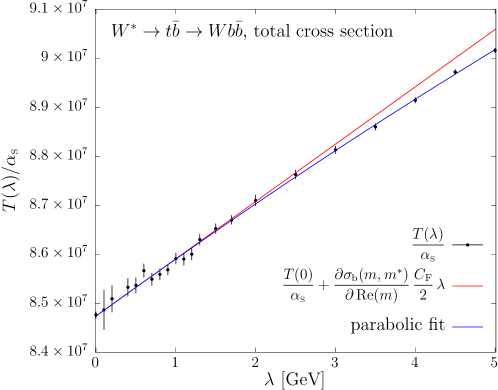
Figure 5.1: Small-$\lambda$ behaviour of $T(\lambda)$ for the total cross section, where $\lambda$ is the gluon mass. In black the data points extracted with our numerical simulations, in red the linear $\lambda$ dependence and in blue the parabolic fit of the points.

As discussed in Sec. 4.7, the same calculation performed in the $\overline{\rm MS}$ mass scheme would yield, for the total cross section, to the replacement given in eq. (4.79)

$$T(\lambda)\to T(\lambda)-\frac{\partial\sigma_{b}}{\partial\,{\rm Re}(m)}\frac{C_{\mathchoice{\displaystyle}{\scriptstyle}{\scriptscriptstyle}{\scriptscriptstyle}\rm F}\alpha_{\mathchoice{\displaystyle}{\scriptstyle}{\scriptscriptstyle}{\scriptscriptstyle}\rm S}}{2}\lambda+{\cal O}(\lambda^{2}).$$ (5.7)

So, in the same figure, we also plot (in red) the expression

$$T(\lambda)=T(0)+\frac{\partial\sigma_{b}}{\partial\,{\rm Re}(m)}\frac{C_{\mathchoice{\displaystyle}{\scriptstyle}{\scriptscriptstyle}{\scriptscriptstyle}\rm F}\alpha_{\mathchoice{\displaystyle}{\scriptstyle}{\scriptscriptstyle}{\scriptscriptstyle}\rm S}}{2}\lambda\,.$$ (5.8)

It is then clear that the $\overline{\rm MS}$ result would have no linear term in $\lambda$ for small $\lambda$, and thus that there is no linear renormalon in this scheme. From the figure it is also clear that this holds for both $\lambda\lesssim\Gamma_{t}$ and for $\lambda\gg\Gamma_{t}$, where $\Gamma_{t}$ is the top width. The $\lambda\lesssim\Gamma_{t}$ behaviour is justified by the fact that, because of the finite width, phase-space points where the top is on shell are never reached (see Appendix D). Thus, no linear renormalon is present unless one uses the pole-mass scheme, that has a linear renormalon in the counterterm.

As far as the $\lambda\gg\Gamma_{t}$ limit, we notice that the $\lambda$ behaviour should be the same as that of the narrow-width approximation (NWA), where the cross section factorizes in terms of the on-shell top-production cross section, and its decay partial width:

$$\sigma\!\left(W^{*}\rightarrow Wb\bar{b}\right)=\sigma\!\left(W^{*}\rightarrow t\bar{b}\right)\frac{\Gamma(t\rightarrow Wb)}{\Gamma_{t}}+\mathcal{O}\left(\frac{\Gamma_{t}}{m}\right).$$ (5.9)

The behaviour of $T(\lambda)$, computed either exactly or in the NWA, is shown in Fig. 5.2.

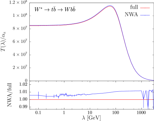
Figure 5.2: $T(\lambda)$ for the NLO total cross section, where $\lambda$ is the gluon mass, computed in the pole-mass scheme using the exact full matrix elements (red) and the narrow-width approximation, NWA (blue).

The factor $\sigma(W^{*}\rightarrow t\bar{b})$ is clearly free of linear renormalons, since it a totally inclusive decay of a colour-neutral system. Although less obvious, this is also the case for the factor $\Gamma(t\rightarrow Wb)$ (see  [10, 52, 33]).

The computation of $T(\lambda)$ using the NWA is discussed in Appendix (C), where we show in Figs. C.1 and C.2 that the linear $\lambda$ behaviour is due to the choice of the pole-mass scheme.

5.1.3 Total cross section with cuts

When the selection cuts discussed earlier are imposed, the cross section depends explicitly upon the jet radius $R$. We expect jets requirement to induce the presence of linear renormalons, and thus linear small-$\lambda$ behaviour of $T$, with a slope that goes like $1/R$ for small $R$ [53, 14].

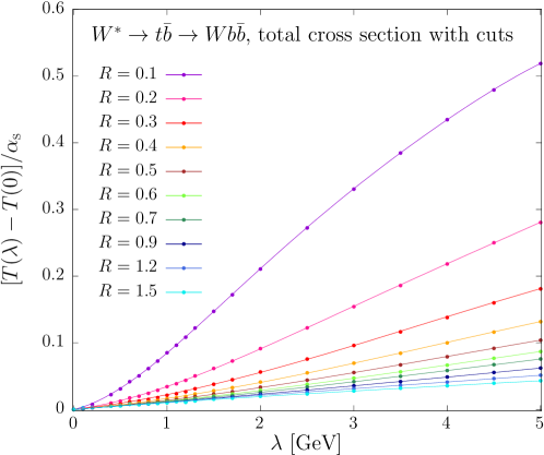
Figure 5.3: Small-$\lambda$ behaviour for $T\!\left(\lambda\right)$ for the total cross section with cuts, for several jet radii. The points represent the data obtained with our numerical calculations, while in solid lines their polynomial fit. The fitting functions are order 5, 4 and 3 polynomials for $R=0.1$, $R=0.2$ and $R\geq 0.3$ radii respectively.

In Fig. 5.3 we display the small-$\lambda$ behaviour for $T(\lambda)$ for the total cross section with cuts, for several jet radii. Together with the results of our simulation, we plot also, for each value of $R$, a polynomial fit to the data.

When changing from the pole to the $\overline{\rm MS}$-mass scheme, we only expect a mild $R$ dependent correction to the slope of $T(\lambda)$ at $\lambda=0$, and thus we cannot expect the same benefit that we observed for the cross section without cuts.

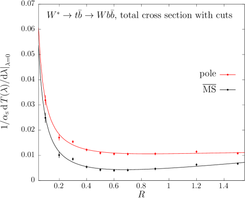
Figure 5.4: $R$ dependence of the slope of $T(\lambda)$ for the total cross section, at $\lambda=0$, using the pole (red) or the $\overline{\rm MS}$ mass scheme (black). The solid lines represent fits of parametric form $a/R+b+c\,R+d\,R^{2}$.

This is illustrated in Fig. 5.4 for several jet radii. The $1/R$ behaviour is clearly visible. In addition, for relatively large-$R$ values, the use of the $\overline{\rm MS}$ scheme brings about some reduction to the slope of the linear term. This may be due to the fact that the cross section with cuts captures a good part of the cross section without cuts, and thus it partially inherits its benefits when changing scheme. However, it is also clear that linear non-perturbative ambiguities remain important also in the $\overline{\rm MS}$ scheme when cuts are involved.

5.2 Reconstructed-top mass

In this section we consider the average value $\langle M\rangle$, where $M$ is the mass of the system comprising the $W$ boson and the $b$ jet. Such an observable is closely related to the top mass, and, on the other hand, is simple enough to be easily computed in our framework. We use the same selection cuts described previously.

We computed $\langle M\rangle$ also in the narrow width limit, by simply setting the top width to 0.001 GeV. In this limit, top production and decay factorize, so that we have an unambiguous assignment of the final state partons to the top decay products. We first compute $\langle M\rangle$ in the narrow width limit, using only the top decay products, and without applying any cuts. We then compute it again, still using only the top decay products, but introducing our standard cuts. Finally we compute it again using all decay products and our standard cuts.

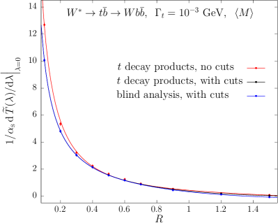
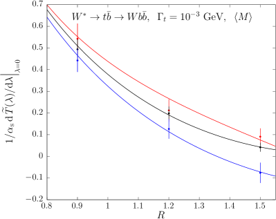
Figure 5.5: $R$ dependence of the slope of $\widetilde{T}(\lambda)$, computed with $\Gamma_{t}=10^{-3}$ GeV, for the averaged reconstructed mass $M$, when using only the top decay products and no cuts (red), when using only the top decay products and applying our cuts (black) and when using all final-state particles and applying our selection cuts (blue). The solid lines are the result of a fit of the form $a/R+b+c\,R+d\,R^{2}$. The black and the blue curves are almost completely overlapping and are indistinguishable in the plot on the left. A blowup of the high-$R$ region is illustrated in the plot on the right.

The results of these calculations are reported in Fig. 5.5, where the slope at $\lambda=0$ of $\widetilde{T}$ for our observable is plotted as a function of the jet radius $R$. As expected we see the shape proportional to $1/R$ for small $R$ [53, 14].

In the case of the calculation of $\langle M\rangle$ performed using only the top decay products, and without any cuts, we expect that, for large values of $R$, the average value of $M$ should get closer and closer to the input top pole mass, irrespective of the value of $\lambda$. Thus, the slope of $\widetilde{T}\!\left(\lambda\right)$ for $\lambda=0$ should become smaller and smaller. We find in this case that, for the largest value of $R$ we are using ($R=1.5$), the slope has a value around 0.09. When cuts are introduced this value becomes even smaller, around 0.04. This curve is fairly close to the one obtained using all final-state particles and including cuts. The large-$R$ value in this case is $-0.08$.

If we change scheme from the pole mass to the $\overline{\rm MS}$ one, the corresponding change of $\widetilde{T}$ is given by eq. (4.80), and for the observable at hand the derivative term it is very near 1. The change in slope when going to the $\overline{\rm MS}$ scheme is roughly $-C_{\mathchoice{\displaystyle}{\scriptstyle}{\scriptscriptstyle}{\scriptscriptstyle}\rm F}/2\approx-0.67$. Thus, if we insisted in using the $\overline{\rm MS}$ mass for the present observable, for large jet-radius parameters, we would get an ambiguity larger than if we used the pole mass scheme. The same holds even if we employ a finite top width. The $R$ dependence of the $\widetilde{T}(\lambda)$ slope for $\Gamma_{t}=1.3279$ GeV is shown in Fig. 5.6.

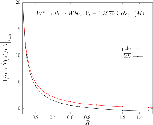
Figure 5.6: $R$ dependence of the slope of $\widetilde{T}(\lambda)$ for the averaged reconstructed mass $M$. The solid lines are the result of a fit of the form $a/R+b+c\,R+d\,R^{2}$.

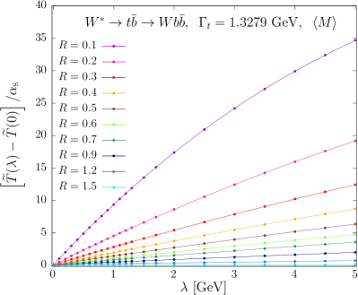
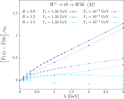
Figure 5.7: Small-$\lambda$ behaviour of $\widetilde{T}(\lambda)$ for the averaged reconstructed-top mass, for several values of the jet radius $R$. In the left pane, the results obtained with $\Gamma_{t}=1.3279$ GeV are shown. The solid lines represent the polynomial fit of the points. For $R\geq 1.2$ a $4^{\rm th}$ order polynomial is adopted, while for the other $R$ values a $5^{\rm th}$ order polynomial is employed. In the right pane, only the results corresponding to large jet radii are displayed, together with the ones obtained with $\Gamma_{t}=10^{-3}$, that are interpolated with a cubic fit (dashed lines).

We notice that, in the present case, for values of $R$ below 1, the $\overline{\rm MS}$ scheme seems to be better, because of a cancellation of the $R$ dependent renormalon and the mass one. From our study, however, it clearly emerges that such cancellation is accidental, and one should not rely upon it to claim an increase in accuracy.

In the left pane of Fig. 5.7 we plot the small-$\lambda$ behaviour of $\widetilde{T}(\lambda)$ for the reconstructed-top mass, computed with the finite top width, for several values of the jet radius $R$. It is clear that our observable is strongly affected by the jet renormalon. The same plot for only the three largest values of $R$ is shown in the right pane. The figure shows clearly that the $\lambda$ slope computed with $\Gamma_{t}=1.3279$ GeV changes when $\lambda$ goes below $1$ GeV, that is to say, when it goes below the top width. This behaviour is expected, since the top width act as a cutoff on soft radiation. In the figure we also report the $\lambda$ behaviour in the narrow-width approximation. It is evident that the slopes computed in this limit are similar to the slopes with $\Gamma_{t}=1.3279$ GeV, for values of $\lambda$ larger than the top width. It is also clear that the slopes that we find here for the largest $R$ value are considerably smaller than the slope change induced by a change to a short distance mass scheme, that amounts to $-0.67$. In other words, the pole mass scheme is more appropriate for this observable, irrespective of finite width effects.

5.3 $\boldsymbol{W}$ boson energy

In this section we study the behaviour of the average value of the $W$ energy, $E_{\mathchoice{\displaystyle}{\scriptstyle}{\scriptscriptstyle}{\scriptscriptstyle}W}$, since this is another top-mass sensitive observable. This observable is chosen since it is a case of an observable that does not depend upon the jet definition. It can thus be considered to be a representative of pure “leptonic” observables in top-mass measurements. In this study, we do not apply any cut, in order to avoid all possible jet or hadronic biases. Our goal is to see if this observable is free of renormalons in some mass scheme.

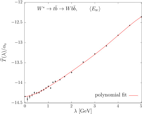
Figure 5.8: Small-$\lambda$ behaviour of $\widetilde{T}(\lambda)$ for $\langle E_{\mathchoice{\displaystyle}{\scriptstyle}{\scriptscriptstyle}{\scriptscriptstyle}W}\rangle$. The solid line represents a $5^{\rm th}$ order polynomial fit.

In order to change scheme, according to eq. (4.80), we need the derivative of the Born value of the observable with respect to the real part of the top mass. We have computed numerically this term and its value is given by

$$\frac{\partial\langle E_{\mathchoice{\displaystyle}{\scriptstyle}{\scriptscriptstyle}{\scriptscriptstyle}W}\rangle_{b}}{\partial\,{\rm Re}(m)}=0.0980\,(8)\,.$$ (5.10)

The small-$\lambda$ dependence of the corresponding $\widetilde{T}$ function is shown in Fig. 5.8: for values of $\lambda$ much larger than the width, the slope of the curve is roughly 0.45. Thus, under these conditions, a renormalon is clearly present whether we use the pole or the $\overline{\rm MS}$ scheme, since the correction in slope due to the use of the latter would be $-0.098\times C_{\mathchoice{\displaystyle}{\scriptstyle}{\scriptscriptstyle}{\scriptscriptstyle}\rm F}/2=-0.065$.

For $\lambda$ below the top width we see a reduction in slope, that is too difficult to estimate because of the lack of statistics. Since the change in slope is clearly related to the top finite width, we carried out the following tests: we run the program with a reduced $\Gamma_{t}$, expecting to see a constant slope extending down to smaller values of $\lambda$. This is illustrated in Fig. 5.9. We clearly see that, as $\Gamma_{t}$ becomes smaller, the slope of the $\lambda$ dependence remains constant, near the value $0.45$ found before, down to smaller values of $\lambda$. Since we have that

$$\frac{\partial\langle E_{\mathchoice{\displaystyle}{\scriptstyle}{\scriptscriptstyle}{\scriptscriptstyle}W}\rangle_{b}}{\partial\,{\rm Re}(m)} = +0.098\,(4)\,,\quad{\rm for}\quad\Gamma_{t}=0.1\leavevmode\nobreak\ {\rm GeV},$$ (5.11)

$$\frac{\partial\langle E_{\mathchoice{\displaystyle}{\scriptstyle}{\scriptscriptstyle}{\scriptscriptstyle}W}\rangle_{b}}{\partial\,{\rm Re}(m)} = +0.10\,(3)\,,\phantom{0}\quad{\rm for}\quad\Gamma_{t}=0.01\leavevmode\nobreak\ {\rm GeV},$$ (5.12)

it is clear that, for a vanishing top width, the $\overline{\rm MS}$ scheme, as well as the pole scheme, is still affected by the presence of a linear renormalon.

We also performed a run with $\Gamma_{t}=10$ GeV and $\Gamma_{t}=20$ GeV, in order to estimate more accurately the value of the slope for $\lambda\ll\Gamma_{t}$. The result is shown in Fig. 5.10. In Tab. 5.1 we illustrate the slopes of $\widetilde{T}(\lambda)$ for small $\lambda$, obtained from the polynomial interpolation displayed in Fig. 5.10, and the corresponding value in the $\overline{\rm MS}$ scheme, obtained by adding $-\frac{C_{\mathchoice{\displaystyle}{\scriptstyle}{\scriptscriptstyle}{\scriptscriptstyle}\rm F}}{2}\frac{\partial\langle E_{\mathchoice{\displaystyle}{\scriptstyle}{\scriptscriptstyle}{\scriptscriptstyle}W}\rangle_{b}}{\partial\,{\rm Re}(m)}$ to the fitted slope. This shows that the linear sensitivity largely cancels in the $\overline{\rm MS}$ scheme.

One may now wonder if the cancellation of the linear sensitivity in the $\overline{\rm MS}$ scheme is exact, or just accidental. In fact, we show in App. D that the cancellation is exact.

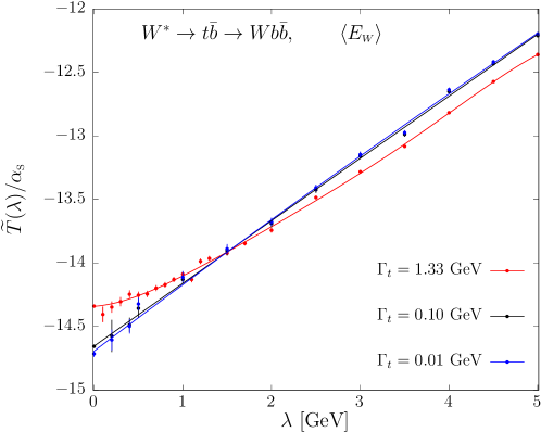
Figure 5.9: Small-$\lambda$ behaviour of $\widetilde{T}(\lambda)$ for $\langle E_{\mathchoice{\displaystyle}{\scriptstyle}{\scriptscriptstyle}{\scriptscriptstyle}W}\rangle$, for increasingly smaller values of $\Gamma_{t}$. The blue and the black solid lines are given by a parabolic fit, the red line is the same one displayed in Fig. 5.8.

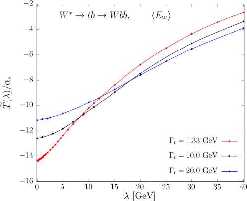
Figure 5.10: Results for the small-$\lambda$ behaviour of $\widetilde{T}$ for $\langle E_{\mathchoice{\displaystyle}{\scriptstyle}{\scriptscriptstyle}{\scriptscriptstyle}W}\rangle$, at different values of $\Gamma_{t}$. The error bar associated to each point computed at a given value of $\lambda$ is also plotted, but is too small to be visible on the scale of the figure. The red line ($\Gamma_{t}=1.33$ GeV) is a $5^{\rm th}$ order polynomial fit for $\lambda\leq 5$ GeV and a spline for larger $\lambda$ values. The blue and the black solid lines, that interpolates the results obtained with $\Gamma_{t}=10$ GeV and $\Gamma_{t}=20$ GeV respectively, are a cubic fit for $\lambda<\Gamma_{t}$ and a spline for $\lambda>\Gamma_{t}$.

$\Gamma_{t}$	slope (pole)	$\displaystyle\frac{\partial\langle E_{\mathchoice{\displaystyle}{\scriptstyle}{\scriptscriptstyle}{\scriptscriptstyle}W}^{\phantom{\big{(}}}\rangle_{b}}{\partial\,{\rm Re}(m)}$	$\displaystyle-\frac{C_{\mathchoice{\displaystyle}{\scriptstyle}{\scriptscriptstyle}{\scriptscriptstyle}\rm F}}{2}\frac{\partial\langle E_{\mathchoice{\displaystyle}{\scriptstyle}{\scriptscriptstyle}{\scriptscriptstyle}W}\rangle_{b}}{\partial\,{\rm Re}(m)}_{\phantom{\big{(}}}$	slope ($\overline{\rm MS}$)
10 GeV	$0.058\,(8)$	$0.0936\,(4)$	$-0.0624\,(3)$	$0.004\,(8)$
20 GeV	$0.061\,(2)$	$0.0901\,(2)$	$-0.0601\,(1)$	$0.001\,(2)$

Table 5.1: Slopes of $\widetilde{T}(\lambda)/\alpha_{\mathchoice{\displaystyle}{\scriptstyle}{\scriptscriptstyle}{\scriptscriptstyle}\rm S}$, evaluated ad $\lambda=0$, computed for $\langle E_{\mathchoice{\displaystyle}{\scriptstyle}{\scriptscriptstyle}{\scriptscriptstyle}W}\rangle$ in the pole-mass scheme and the derivative terms needed to change to the $\overline{\rm MS}$ one, for large top widths.

Chapter 6 All-order expansions in $\boldsymbol{\alpha_{\mathchoice{\displaystyle}{\scriptstyle}{\scriptscriptstyle}{\scriptscriptstyle}\rm S}}$

We will now consider the all-order expansion of various quantities, in order to see how the infrared renormalon affects the large-order behaviour, both in the pole mass scheme and in the $\overline{\rm MS}$ scheme.

One may think that in our framework we may even compare quantities computed in different mass schemes, and thus assess the reliability of the methods used to estimate the resummation of divergent series, and the corresponding ambiguity. In fact, within our large-$n_{f}$ approximation, if the method adopted to resum the perturbative expansion is linear, as is the case of the Borel transform method, we should find identical results (always in the large $n_{f}$ sense) in the $\overline{\rm MS}$ and the pole-mass schemes. This is shown as follows. The relation between the pole and $\overline{\rm MS}$ scheme for a generic observable is given by, following eq. (4.7),

$${\langle O\rangle_{\rm b}}(m,m^{*})+\langle O\rangle^{(1)}(m,m^{*})\alpha_{\mathchoice{\displaystyle}{\scriptstyle}{\scriptscriptstyle}{\scriptscriptstyle}\rm S}=\, {\langle O\rangle_{\rm b}}(\overline{m},\overline{m}^{*})+\bigg{\{}\left[\frac{\partial{\langle O\rangle_{\rm b}}(m,m^{*})}{\partial m}(m-\overline{m})+{\rm cc}\right]$$

$$+\langle O\rangle^{(1)}(m,m^{*})\alpha_{\mathchoice{\displaystyle}{\scriptstyle}{\scriptscriptstyle}{\scriptscriptstyle}\rm S}\bigg{\}}+{\cal O}(\alpha_{\mathchoice{\displaystyle}{\scriptstyle}{\scriptscriptstyle}{\scriptscriptstyle}\rm S}^{2}(\alpha_{\mathchoice{\displaystyle}{\scriptstyle}{\scriptscriptstyle}{\scriptscriptstyle}\rm S}n_{f})^{n}).$$ (6.1)

Neglecting subleading terms, this is an identity, since the expansion of ${\langle O\rangle_{\rm b}}$ in the mass difference stops at the first order in the large-$n_{f}$ limit. When performing the calculation in the pole mass scheme, we need to resum the expansion of $\langle O\rangle^{(1)}$, while if we perform the calculation in the $\overline{\rm MS}$ scheme, we are resumming the expansion of the sum of terms in the curly bracket. If the resummation method is linear this last resummation can be performed on the individual terms inside the curly bracket. This is exactly what we would do on the left-hand side if, after the resummation, we wanted to express the same result in the $\overline{\rm MS}$ scheme. In other words, if one uses the Borel method to perform the resummation, and defines the pole mass to be the sum of the mass relation formula eq. (4.70), all results obtained in the $\overline{\rm MS}$ scheme would be identical to those obtained in the pole mass scheme up to terms of relative order $\alpha_{\mathchoice{\displaystyle}{\scriptstyle}{\scriptscriptstyle}{\scriptscriptstyle}\rm S}C_{\mathchoice{\displaystyle}{\scriptstyle}{\scriptscriptstyle}{\scriptscriptstyle}\rm F}$ or $\alpha_{\mathchoice{\displaystyle}{\scriptstyle}{\scriptscriptstyle}{\scriptscriptstyle}\rm S}C_{\mathchoice{\displaystyle}{\scriptstyle}{\scriptscriptstyle}{\scriptscriptstyle}\rm A}$, provided the same Borel sum method is used also for the observables.

In the following we will try to estimate the terms of the perturbative expansion using our large-$n_{f}$ results. In order to do this, we will perform the replacement $-T_{\mathchoice{\displaystyle}{\scriptstyle}{\scriptscriptstyle}{\scriptscriptstyle}\rm F}/(3\pi)\to b_{0}$ accompanied by some other minor adjustments, as described in Sec. 3.3. Needless to say, with these realistic values, the large-$n_{f}$ approximation breaks down, and terms of relative order $\alpha_{\mathchoice{\displaystyle}{\scriptstyle}{\scriptscriptstyle}{\scriptscriptstyle}\rm S}C_{\mathchoice{\displaystyle}{\scriptstyle}{\scriptscriptstyle}{\scriptscriptstyle}\rm F}$ or $\alpha_{\mathchoice{\displaystyle}{\scriptstyle}{\scriptscriptstyle}{\scriptscriptstyle}\rm S}C_{\mathchoice{\displaystyle}{\scriptstyle}{\scriptscriptstyle}{\scriptscriptstyle}\rm A}$ may be sizeable. We thus expect that by changing scheme we will generate difference of relative orders $\alpha_{\mathchoice{\displaystyle}{\scriptstyle}{\scriptscriptstyle}{\scriptscriptstyle}\rm S}C_{\mathchoice{\displaystyle}{\scriptstyle}{\scriptscriptstyle}{\scriptscriptstyle}\rm F}$ or $\alpha_{\mathchoice{\displaystyle}{\scriptstyle}{\scriptscriptstyle}{\scriptscriptstyle}\rm S}C_{\mathchoice{\displaystyle}{\scriptstyle}{\scriptscriptstyle}{\scriptscriptstyle}\rm A}$, that are not negligible. These differences should not therefore be interpreted as due to large ambiguities related to the choice of mass scheme, but rather to the large-$n_{f}$ approximation.

The procedure we adopt in order to compute the terms of the perturbative expansion follows from eq. (4.64). We fit numerically the $\lambda$ dependence of the appropriate $T$ or $\widetilde{T}$ function, and we take the derivative of the fit. The arctangent factor is instead expanded analytically, and the integration is performed numerically for each perturbative order. In order to have a semi-realistic result for the perturbative coefficients we perform the following replacement

$$\Pi(\lambda^{2}+i\eta,\mu^{2})-\Pi_{\rm ct}=\frac{\alpha_{\mathchoice{\displaystyle}{\scriptstyle}{\scriptscriptstyle}{\scriptscriptstyle}\rm S}T_{\mathchoice{\displaystyle}{\scriptstyle}{\scriptscriptstyle}{\scriptscriptstyle}\rm F}}{3\pi}\left(\frac{5}{3}-\log\frac{\lambda^{2}}{\mu^{2}}+i\pi\right)\equiv\frac{\alpha_{\mathchoice{\displaystyle}{\scriptstyle}{\scriptscriptstyle}{\scriptscriptstyle}\rm S}n_{f}T_{\mathchoice{\displaystyle}{\scriptstyle}{\scriptscriptstyle}{\scriptscriptstyle}\rm R}}{3\pi}\left(\frac{5}{3}-\log\frac{\lambda^{2}}{\mu^{2}}+i\pi\right)$$

$$\to-\frac{\alpha_{\mathchoice{\displaystyle}{\scriptstyle}{\scriptscriptstyle}{\scriptscriptstyle}\rm S}11C_{\mathchoice{\displaystyle}{\scriptstyle}{\scriptscriptstyle}{\scriptscriptstyle}\rm A}}{12\pi}\left(C_{g}-\log\frac{\lambda^{2}}{\mu^{2}}+i\pi\right)+\frac{\alpha_{\mathchoice{\displaystyle}{\scriptstyle}{\scriptscriptstyle}{\scriptscriptstyle}\rm S}n_{l}T_{\mathchoice{\displaystyle}{\scriptstyle}{\scriptscriptstyle}{\scriptscriptstyle}\rm R}}{3\pi}\left(\frac{5}{3}-\log\frac{\lambda^{2}}{\mu^{2}}+i\pi\right),\qquad$$ (6.2)

where $C_{g}$ is given in eq. (3.64). As a consequence, in eqs. (4.64), (4.45), and (3.2) the constant $C$, introduced in eq. (3.12), is replaced with eq. (3.65) and the overall $1/b_{0,f}$ factor with $1/b_{0}=(\frac{\alpha_{\mathchoice{\displaystyle}{\scriptstyle}{\scriptscriptstyle}{\scriptscriptstyle}\rm S}n_{l}T_{\mathchoice{\displaystyle}{\scriptstyle}{\scriptscriptstyle}{\scriptscriptstyle}\rm R}}{3}-\frac{\alpha_{\mathchoice{\displaystyle}{\scriptstyle}{\scriptscriptstyle}{\scriptscriptstyle}\rm S}11C_{\mathchoice{\displaystyle}{\scriptstyle}{\scriptscriptstyle}{\scriptscriptstyle}\rm A}}{12})^{-1}$. For the computation of our observables no further modification is required, since the factors $\Delta(\lambda)$ of eq. (4.69) and $\widetilde{\Delta}(\lambda)$ of eq. (4.69) do not depend on $n_{f}$, that cancels in the ratio $\sigma_{q\bar{q}}^{(2)}/b_{0,f}$.

However, given the fact that the pole-$\overline{\rm MS}$ mass relation involves ultraviolet divergent quantities, it must be carried out in $d=4-2\epsilon$ dimension. For this reason, in this case, we cannot simply use the $\mathcal{O}(\epsilon^{0})$ expansion of $\left[\Pi(\lambda^{2}+i\eta,\mu^{2})-\Pi_{\rm ct}\right]$ given in eq. (6.2) to evaluate eqs. (3.43) and (3.46), but we need to use eqs. (3.58) and (3.59). We remark that these contributions do not contain any infrared renormalon, conversely to $r_{f}(m,\mu,\alpha_{\mathchoice{\displaystyle}{\scriptstyle}{\scriptscriptstyle}{\scriptscriptstyle}\rm S})$, that can be computed in $d=4$ dimensions. For this reason, as already discussed in Sec. 3.3, the presence of a second term $C_{g}^{\prime}\epsilon^{2}$, that accompanies $C_{g}\epsilon$ in eq. (3.58), is totally negligible for the estimate of the leading linear renormalons.

6.1 Mass-conversion formula

The procedure for the calculation of the mass-conversion formula is described in Sec. 3.2. Here we switch to the realistic $b_{0}$ and $C$ values as discussed in the previous section. The expansion of the mass conversion formula reads

$$\overline{m}(\mu)=m\left(1-\sum_{i=1}^{\infty}c_{i}\,\alpha_{\mathchoice{\displaystyle}{\scriptstyle}{\scriptscriptstyle}{\scriptscriptstyle}\rm S}^{i}\right)\,,$$ (6.3)

and the $c_{i}$ coefficients are tabulated in Tab. 6.1, with $\mu^{2}={\rm Re}(m^{2})=m_{0}^{2}$, where $m_{0}$ is given in eq. (4.1).

$\displaystyle\phantom{\Big{|}}m-\overline{m}(\mu)\phantom{\Big{|}}$
$\phantom{\Big{|}}i\phantom{\Big{|}}$	${\rm Re}\left(c_{i}\right)$	${\rm Im}\left(c_{i}\right)$	${\rm Re}\left(m\,c_{i}\,\alpha_{\mathchoice{\displaystyle}{\scriptstyle}{\scriptscriptstyle}{\scriptscriptstyle}\rm S}^{i}\right)$	${\rm Im}\left(m\,c_{i}\,\alpha_{\mathchoice{\displaystyle}{\scriptstyle}{\scriptscriptstyle}{\scriptscriptstyle}\rm S}^{i}\right)$
$\phantom{\Big{|}}1\phantom{\Big{|}}$	$4.244\times 10^{-1}$	$2.450\times 10^{-3}$	$7.919\times 10^{+0}$	$+1.524\times 10^{-2}$
$\phantom{\Big{|}}2\phantom{\Big{|}}$	$6.437\times 10^{-1}$	$2.094\times 10^{-3}$	$1.299\times 10^{+0}$	$-7.729\times 10^{-4}$
$\phantom{\Big{|}}3\phantom{\Big{|}}$	$1.968\times 10^{+0}$	$8.019\times 10^{-3}$	$4.297\times 10^{-1}$	$+9.665\times 10^{-5}$
$\phantom{\Big{|}}4\phantom{\Big{|}}$	$7.231\times 10^{+0}$	$2.567\times 10^{-2}$	$1.707\times 10^{-1}$	$-5.110\times 10^{-5}$
$\phantom{\Big{|}}5\phantom{\Big{|}}$	$3.497\times 10^{+1}$	$1.394\times 10^{-1}$	$8.930\times 10^{-2}$	$+1.240\times 10^{-5}$
$\phantom{\Big{|}}6\phantom{\Big{|}}$	$2.174\times 10^{+2}$	$8.164\times 10^{-1}$	$6.005\times 10^{-2}$	$-5.616\times 10^{-6}$
$\phantom{\Big{|}}7\phantom{\Big{|}}$	$1.576\times 10^{+3}$	$6.133\times 10^{+0}$	$4.709\times 10^{-2}$	$+2.009\times 10^{-6}$
$\phantom{\Big{|}}8\phantom{\Big{|}}$	$1.354\times 10^{+4}$	$5.180\times 10^{+1}$	$4.376\times 10^{-2}$	$-1.031\times 10^{-6}$
$\phantom{\Big{|}}9\phantom{\Big{|}}$	$1.318\times 10^{+5}$	$5.087\times 10^{+2}$	$4.608\times 10^{-2}$	$+4.961\times 10^{-7}$
$\phantom{\Big{|}}10\phantom{\Big{|}}$	$1.450\times 10^{+6}$	$5.572\times 10^{+3}$	$5.481\times 10^{-2}$	$-2.909\times 10^{-7}$

Table 6.1: Real and imaginary parts of the coefficients $c_{i}$ of the mass relation (6.3), up to the tenth order in the strong coupling constant $\alpha_{\mathchoice{\displaystyle}{\scriptstyle}{\scriptscriptstyle}{\scriptscriptstyle}\rm S}(\mu)$, with $\mu^{2}={\rm Re}(m^{2})$ and $m=172.5$ GeV. The numbers shown in the last two columns are expressed in GeV.

Since we are using the complex mass scheme, they are complex, with a small imaginary part, and they have a slight dependence upon the ratio $\Gamma_{t}/{\rm Re}(m)$. For small $\Gamma_{t}$ they become independent on $m$ and $\Gamma_{t}$, and their imaginary part vanishes.

The value of the $\overline{\rm MS}$ mass we adopt in the following is found by truncating the series in eq. 6.3 at the smallest term before the series starts diverging, that corresponds to $i=8$, as shown in Tab. 6.1. We thus find that for a complex pole mass

$$m=(172.50-0.66\,i)\leavevmode\nobreak\ {\rm GeV}$$ (6.4)

the value of the corresponding $\overline{\rm MS}$ complex mass is

$$\overline{m}(\mu)=m\left(1-\sum_{i=1}^{8}c_{i}\,\alpha_{\mathchoice{\displaystyle}{\scriptstyle}{\scriptscriptstyle}{\scriptscriptstyle}\rm S}^{i}\right)\ =(162.44-0.68\,i)\leavevmode\nobreak\ {\rm GeV},$$ (6.5)

with $\mu=\sqrt{{\rm Re}(m^{2})}$.

6.2 The total cross section

In this section we deal with the perturbative expansion of the total cross section, first without cuts, and then with cuts.

6.2.1 Total cross section without cuts

As discussed in Sec. 5.1.2, $T(\lambda)$ (4.47) for the total cross section does not have any term linear in $\lambda$, if expressed in terms of the $\overline{\rm MS}$ mass. It follows that the total cross section computed in the $\overline{\rm MS}$ scheme should not have any $\Lambda_{\mathchoice{\displaystyle}{\scriptstyle}{\scriptscriptstyle}{\scriptscriptstyle}\rm QCD}/\overline{m}$ renormalon and should display a better behavior at large orders.

	$\phantom{\Big{|}}\sigma/\sigma^{\rm nocuts}_{\rm b}(m{})\phantom{\Big{|}}$
	—pole scheme —		$\overline{\rm MS}$ scheme
$\phantom{\Big{|}}i\phantom{\Big{|}}$	$c_{i}$	$c_{i}\,\alpha_{\mathchoice{\displaystyle}{\scriptstyle}{\scriptscriptstyle}{\scriptscriptstyle}\rm S}^{i}$	$c_{i}$	$c_{i}\,\alpha_{\mathchoice{\displaystyle}{\scriptstyle}{\scriptscriptstyle}{\scriptscriptstyle}\rm S}^{i}$
0	1.00000000	1.0000000	0.86841331	0.8684133
1	$5.003\,(0)\times 10^{-1}$	$5.411\,(0)\times 10^{-2}$	$1.480\,(0)\times 10^{0}$	$1.601\,(0)\times 10^{-1}$
2	$-6.20\,(2)\times 10^{-1}$	$-7.25\,(2)\times 10^{-3}$	$4.42\,(2)\times 10^{-1}$	$5.17\,(2)\times 10^{-3}$
3	$-3.03\,(2)\times 10^{0}$	$-3.83\,(3)\times 10^{-3}$	$6.4\,(2)\times 10^{-1}$	$8.1\,(3)\times 10^{-4}$
4	$-1.25\,(2)\times 10^{1}$	$-1.70\,(3)\times 10^{-3}$	$0\,(2)\times 10^{-2}$	$0\,(3)\times 10^{-6}$
5	$-6.4\,(2)\times 10^{1}$	$-9.4\,(3)\times 10^{-4}$	$1\,(2)\times 10^{-1}$	$1\,(3)\times 10^{-5}$
6	$-3.9\,(1)\times 10^{2}$	$-6.2\,(2)\times 10^{-4}$	$0\,(1)\times 10^{0}$	$0\,(2)\times 10^{-6}$
7	$-2.9\,(1)\times 10^{3}$	$-5.0\,(2)\times 10^{-4}$	$0\,(1)\times 10^{1}$	$0\,(2)\times 10^{-6}$
8	$-2.5\,(1)\times 10^{4}$	$-4.6\,(2)\times 10^{-4}$	$0\,(1)\times 10^{2}$	$0\,(2)\times 10^{-6}$
9	$-2.4\,(1)\times 10^{5}$	$-4.9\,(2)\times 10^{-4}$	$0\,(1)\times 10^{3}$	$0\,(2)\times 10^{-6}$
10	$-2.6\,(1)\times 10^{6}$	$-5.8\,(2)\times 10^{-4}$	$0\,(1)\times 10^{4}$	$-1\,(2)\times 10^{-6}$

Table 6.2: Coefficients of the $\alpha_{\mathchoice{\displaystyle}{\scriptstyle}{\scriptscriptstyle}{\scriptscriptstyle}\rm S}$ expansion of the inclusive cross section to all orders, computed in the large-$b_{0}$ limit, normalized to the Born cross section computed in the pole-mass scheme. The errors reported in parenthesis are due to the uncertainty on the linear coefficient of the fit (i.e. $p_{1}$ in eq. (4.54)).

The coefficients $c_{i}$ of the expansion of eq. (4.45) in terms of $\alpha_{\mathchoice{\displaystyle}{\scriptstyle}{\scriptscriptstyle}{\scriptscriptstyle}\rm S}$

$$\sigma=\sigma_{\rm b}^{\rm nocuts}(m)\left(c_{0}+\sum_{i=1}^{\infty}c_{i}\,\alpha_{\mathchoice{\displaystyle}{\scriptstyle}{\scriptscriptstyle}{\scriptscriptstyle}\rm S}^{i}\right)$$ (6.6)

are collected in Tab. 6.2, in the pole (left) and in the $\overline{\rm MS}$ (right) schemes. At large orders, the $\overline{\rm MS}$ total cross section receives much smaller contributions. On the other hand we see that the $\rm N^{3}LO$ contribution to $\sigma(m)$ is already affected by a factorial growth. The minimum of the series is reached for $i=8$ (that corresponds to an $\mathcal{O}(\alpha_{\mathchoice{\displaystyle}{\scriptstyle}{\scriptscriptstyle}{\scriptscriptstyle}\rm S}^{8})$ correction), and it is two orders of magnitude larger than the corresponding contribution computed in the $\overline{\rm MS}$ scheme. We also notice that the $\overline{\rm MS}$ result has an NLO correction larger than the pole mass result, an NNLO correction that is similar, and smaller N³LO and higher order corrections. We also expect that the apparent convergence of the expansion for the first few orders should depend upon the available phase space for radiation.

6.2.2 Total cross section with cuts

As we have seen in Sec. 5.1.3, the presence of selection cuts introduces a renormalon in the total cross section whose magnitude goes like $1/R$.

	$\phantom{\Big{|}}\sigma/\sigma^{\rm nocuts}_{\rm b}(m{})\;\;R=0.1\phantom{\Big{|}}$
	—pole scheme —	$\overline{\rm MS}$ scheme
$\phantom{\Big{|}}i\phantom{\Big{|}}$	$c_{i}\,\alpha_{\mathchoice{\displaystyle}{\scriptstyle}{\scriptscriptstyle}{\scriptscriptstyle}\rm S}^{i}$	$c_{i}\,\alpha_{\mathchoice{\displaystyle}{\scriptstyle}{\scriptscriptstyle}{\scriptscriptstyle}\rm S}^{i}$
0	0.9985836	0.8666708
1	$-7.953\,(0)\times 10^{-2}$	$2.650\,(0)\times 10^{-2}$
2	$-7.22\,(2)\times 10^{-2}$	$-5.98\,(2)\times 10^{-2}$
3	$-3.71\,(2)\times 10^{-2}$	$-3.24\,(2)\times 10^{-2}$
4	$-1.97\,(2)\times 10^{-2}$	$-1.80\,(2)\times 10^{-2}$
5	$-1.13\,(2)\times 10^{-2}$	$-1.04\,(2)\times 10^{-2}$
6	$-7.0\,(2)\times 10^{-3}$	$-6.4\,(2)\times 10^{-3}$
7	$-4.8\,(1)\times 10^{-3}$	$-4.3\,(1)\times 10^{-3}$
8	$-3.6\,(1)\times 10^{-3}$	$-3.1\,(1)\times 10^{-3}$
9	$-3.1\,(1)\times 10^{-3}$	$-2.7\,(1)\times 10^{-3}$
10	$-3.2\,(2)\times 10^{-3}$	$-2.6\,(2)\times 10^{-3}$

	$\phantom{\Big{|}}\sigma/\sigma^{\rm nocuts}_{\rm b}(m{})\;\;R=0.5\phantom{\Big{|}}$
	—pole scheme —	$\overline{\rm MS}$ scheme
$\phantom{\Big{|}}i\phantom{\Big{|}}$	$c_{i}\,\alpha_{\mathchoice{\displaystyle}{\scriptstyle}{\scriptscriptstyle}{\scriptscriptstyle}\rm S}^{i}$	$c_{i}\,\alpha_{\mathchoice{\displaystyle}{\scriptstyle}{\scriptscriptstyle}{\scriptscriptstyle}\rm S}^{i}$
0	0.9783310	0.8511828
1	$-4.992\,(0)\times 10^{-3}$	$9.705\,(0)\times 10^{-2}$
2	$-2.966\,(5)\times 10^{-2}$	$-1.779\,(5)\times 10^{-2}$
3	$-1.267\,(6)\times 10^{-2}$	$-8.22\,(6)\times 10^{-3}$
4	$-5.37\,(6)\times 10^{-3}$	$-3.73\,(6)\times 10^{-3}$
5	$-2.58\,(5)\times 10^{-3}$	$-1.66\,(5)\times 10^{-3}$
6	$-1.44\,(4)\times 10^{-3}$	$-8.5\,(4)\times 10^{-4}$
7	$-9.8\,(4)\times 10^{-4}$	$-5.0\,(4)\times 10^{-4}$
8	$-8.1\,(4)\times 10^{-4}$	$-3.7\,(4)\times 10^{-4}$
9	$-8.0\,(4)\times 10^{-4}$	$-3.4\,(4)\times 10^{-4}$
10	$-9.2\,(5)\times 10^{-4}$	$-3.7\,(5)\times 10^{-4}$

Table 6.3: Values of the $c_{i}\,\alpha_{\mathchoice{\displaystyle}{\scriptstyle}{\scriptscriptstyle}{\scriptscriptstyle}\rm S}^{i}$ terms of the perturbative expansion for the average value of the cross section with cuts, normalized to the inclusive Born cross section computed in the pole-mass scheme (see eq. (6.6)), for two different values of the jet radius ($R=0.1$ in the left pane and $R=0.5$ in the right one). The errors reported in parenthesis are due to the uncertainty on the linear coefficient of the fit (i.e. $p_{1}$ in eq. (4.54)).

In Tab. 6.3 we present the results for the total cross section, in the pole and in the $\overline{\rm MS}$-mass scheme, for a small jet radius, $R=0.1$, and a more realistic value, $R=0.5$. For small radii, the perturbative expansion displays roughly the same bad behaviour, either when we use the pole or the $\overline{\rm MS}$ scheme. For larger values of $R$, the size of the coefficients are typically smaller than the corresponding ones with smaller values or $R$. In particular if we compare the coefficients for $R=0.1$ and $R=0.5$, the second ones are one order of magnitude smaller than the first ones. Furthermore, for $R=0.5$, the coefficients computed in the $\overline{\rm MS}$-mass scheme are roughly half of the ones computed in the pole-mass scheme. As remarked earlier, this reduction is due to an accidental cancellation of the pole-mass associated renormalon and the $1/R$, jet related one, and cannot be used to imply that the $\overline{\rm MS}$ scheme should be favoured in this case.

6.3 Reconstructed-top mass

In this section, we discuss the terms of the perturbative expansion for the average reconstructed mass $\langle M\rangle$

$$\langle M\rangle=\sum_{i=0}^{\infty}c_{i}\,\alpha_{\mathchoice{\displaystyle}{\scriptstyle}{\scriptscriptstyle}{\scriptscriptstyle}\rm S}^{i}\,,$$ (6.7)

for three values of the $R$ parameter. We apply the cuts described in Sec. 5.1 and the results are collected in Tab. 6.4.

	$\langle M\rangle$ [GeV]
	$\phantom{\Big{|}}R=0.1\phantom{\Big{|}}$		$\phantom{\Big{|}}R=0.5\phantom{\Big{|}}$		$\phantom{\Big{|}}R=1.5\phantom{\Big{|}}$
$i$	— pole —	$\overline{\rm MS}$	— pole—	$\overline{\rm MS}$	— pole —	$\overline{\rm MS}$
0	$172.8280$	$163.0146$	$172.8201$	$163.0040$	$172.7533$	$162.9244$
1	$-7.597\,(0)\times 10^{0}$	$2.163\,(0)\times 10^{-1}$	$-2.785\,(0)\times 10^{0}$	$5.030\,(0)\times 10^{0}$	$4.446\,(0)\times 10^{-1}$	$8.268\,(0)\times 10^{0}$
2	$-4.136\,(2)\times 10^{0}$	$-2.852\,(2)\times 10^{0}$	$-1.255\,(1)\times 10^{0}$	$2.9\,(1)\times 10^{-2}$	$1.029\,(8)\times 10^{-1}$	$1.387\,(1)\times 10^{0}$
3	$-2.397\,(2)\times 10^{0}$	$-1.973\,(2)\times 10^{0}$	$-5.96\,(2)\times 10^{-1}$	$-1.72\,(2)\times 10^{-1}$	$1.4\,(1)\times 10^{-2}$	$4.38\,(1)\times 10^{-1}$
4	$-1.505\,(2)\times 10^{0}$	$-1.337\,(2)\times 10^{0}$	$-3.13\,(2)\times 10^{-1}$	$-1.44\,(2)\times 10^{-1}$	$-6\,(1)\times 10^{-3}$	$1.63\,(1)\times 10^{-1}$
5	$-1.038\,(2)\times 10^{0}$	$-9.50\,(2)\times 10^{-1}$	$-1.88\,(2)\times 10^{-1}$	$-1.00\,(2)\times 10^{-2}$	$-9.7\,(9)\times 10^{-3}$	$7.86\,(9)\times 10^{-2}$
6	$-7.94\,(2)\times 10^{-1}$	$-7.35\,(2)\times 10^{-1}$	$-1.33\,(1)\times 10^{-1}$	$-7.3\,(1)\times 10^{-2}$	$-1.05\,(8)\times 10^{-2}$	$4.89\,(8)\times 10^{-2}$
7	$-6.79\,(2)\times 10^{-1}$	$-6.33\,(2)\times 10^{-1}$	$-1.09\,(1)\times 10^{-1}$	$-6.3\,(1)\times 10^{-2}$	$-1.12\,(7)\times 10^{-2}$	$3.53\,(7)\times 10^{-2}$
8	$-6.51\,(2)\times 10^{-1}$	$-6.08\,(2)\times 10^{-1}$	$-1.04\,(1)\times 10^{-1}$	$-6.1\,(1)\times 10^{-2}$	$-1.25\,(7)\times 10^{-2}$	$3.08\,(7)\times 10^{-2}$
9	$-6.99\,(2)\times 10^{-1}$	$-6.54\,(2)\times 10^{-1}$	$-1.12\,(1)\times 10^{-1}$	$-6.7\,(1)\times 10^{-2}$	$-1.47\,(7)\times 10^{-2}$	$3.09\,(7)\times 10^{-2}$
10	$-8.37\,(2)\times 10^{-1}$	$-7.83\,(2)\times 10^{-1}$	$-1.35\,(1)\times 10^{-1}$	$-8.1\,(1)\times 10^{-2}$	$-1.85\,(9)\times 10^{-2}$	$3.57\,(9)\times 10^{-2}$

Table 6.4: Values of the $c_{i}\,\alpha_{\mathchoice{\displaystyle}{\scriptstyle}{\scriptscriptstyle}{\scriptscriptstyle}\rm S}^{i}$ terms of the perturbative expansion for the average value of the reconstructed-top mass, defined in eq. (6.7), for three different jet radii in the pole-mass and $\overline{\rm MS}$-mass scheme. The errors reported in parenthesis are due to the uncertainty on the linear coefficient of the fit (i.e. $p_{1}$ in eq. (4.54)).

From the table we can see that, for very small jet radii, the asymptotic character of the perturbative expansion is manifest in both the pole and $\overline{\rm MS}$ scheme. For the realistic value $R=0.5$, the $\overline{\rm MS}$ scheme seems to behave slightly better. In fact, this is only a consequence of the fact that the jet-renormalon and the mass-renormalon corrections have opposite signs, with the mass correction in the $\overline{\rm MS}$ scheme largely prevailing at small orders, yielding positive effects.

As the radius becomes very large, the jet renormalon becomes less and less pronounced, in the pole-mass scheme, leading to smaller corrections at all orders. This is consistent with the discussion given in Sec. 5.2, where we have seen that, for large radii, the reconstructed mass becomes strongly related to the top pole mass, since it approaches what one would reconstruct from the “true” top decay products.

6.4 $\boldsymbol{W}$ boson energy

The coefficients of the perturbative expansion of the average energy of the $W$ boson in the pole and $\overline{\rm MS}$ schemes

$$\langle E_{\mathchoice{\displaystyle}{\scriptstyle}{\scriptscriptstyle}{\scriptscriptstyle}W}\rangle=\sum_{i=0}^{\infty}c_{i}\,\alpha_{\mathchoice{\displaystyle}{\scriptstyle}{\scriptscriptstyle}{\scriptscriptstyle}\rm S}^{i}.$$ (6.8)

are displayed in Tab. 6.5. We notice that the perturbative expansions are similarly behaved in both schemes up to $i\approx 6$, while, for higher orders, the $\overline{\rm MS}$ scheme result is clearly better convergent. This supports the observation, done in Sec. 5.3, that the top width screens the renormalon effect if the $\overline{\rm MS}$ mass is used. In fact, the $6^{\rm th}$ order renormalon contribution is dominated by scales of order $m_{t}\,e^{-5}\approx 1.16$, as illustrated in Sec. 2.3, very near the top width.

By looking at the $i=0$ row, we notice that a variation of roughly 10 GeV in the value of the top mass, corresponding to the pole-$\overline{\rm MS}$ mass difference, leads to a variation of less than 1 GeV in $\langle E_{\mathchoice{\displaystyle}{\scriptstyle}{\scriptscriptstyle}{\scriptscriptstyle}W}\rangle_{b}$. This implies that the sensitivity of the $W$-boson energy $E_{\mathchoice{\displaystyle}{\scriptstyle}{\scriptscriptstyle}{\scriptscriptstyle}W}$ to the top mass is much weaker than for the reconstructed-top mass $M$. Indeed, in Secs. 5.2 and 5.3 we already noticed that

$$\frac{\partial\langle E_{\mathchoice{\displaystyle}{\scriptstyle}{\scriptscriptstyle}{\scriptscriptstyle}W}\rangle_{b}}{\partial\,{\rm Re}(m)}\approx 0.1\,,\qquad\frac{\partial\langle M\rangle_{b}}{\partial\,{\rm Re}(m)}\approx 1.$$ (6.9)

The value of the $E_{\mathchoice{\displaystyle}{\scriptstyle}{\scriptscriptstyle}{\scriptscriptstyle}W}$ derivative is strongly affected by our choice of the rest frame energy $E=300$ GeV, that corresponds to a boost $\beta_{\mathchoice{\displaystyle}{\scriptstyle}{\scriptscriptstyle}{\scriptscriptstyle}top}=|\vec{p}_{\mathchoice{\displaystyle}{\scriptstyle}{\scriptscriptstyle}{\scriptscriptstyle}top}|/E_{\mathchoice{\displaystyle}{\scriptstyle}{\scriptscriptstyle}{\scriptscriptstyle}top}=0.5$ for an on-shell top-quark. Thus, despite the fact that $E_{\mathchoice{\displaystyle}{\scriptstyle}{\scriptscriptstyle}{\scriptscriptstyle}W}$ is free from physical renormalons, if the top quark has substantial kinetic energy, the weak sensitivity of such observable to the value of the top mass may in practice reduce the precision of the measurement.

	$\displaystyle\langle E_{W}\rangle$    [GeV]
	—pole scheme —		$\overline{\rm MS}$ scheme
$\phantom{\Big{|}}i\phantom{\Big{|}}$	$c_{i}$	$c_{i}\,\alpha_{\mathchoice{\displaystyle}{\scriptstyle}{\scriptscriptstyle}{\scriptscriptstyle}\rm S}^{i}$	$c_{i}$	$c_{i}\,\alpha_{\mathchoice{\displaystyle}{\scriptstyle}{\scriptscriptstyle}{\scriptscriptstyle}\rm S}^{i}$
0	$121.5818$	$121.5818$	$120.8654$	$120.8654$
1	$-1.435\,(0)\times 10^{1}$	$-1.552\,(0)\times 10^{0}$	$-7.192\,(0)\times 10^{0}$	$-7.779\,(0)\times 10^{-1}$
2	$-4.97\,(4)\times 10^{1}$	$-5.82\,(4)\times 10^{-1}$	$-3.88\,(4)\times 10^{1}$	$-4.54\,(4)\times 10^{-1}$
3	$-1.79\,(5)\times 10^{2}$	$-2.26\,(6)\times 10^{-1}$	$-1.45\,(5)\times 10^{2}$	$-1.84\,(6)\times 10^{-1}$
4	$-6.9\,(4)\times 10^{2}$	$-9.4\,(6)\times 10^{-2}$	$-5.7\,(4)\times 10^{2}$	$-7.8\,(6)\times 10^{-2}$
5	$-2.9\,(3)\times 10^{3}$	$-4.4\,(5)\times 10^{-2}$	$-2.4\,(3)\times 10^{3}$	$-3.5\,(5)\times 10^{-2}$
6	$-1.4\,(3)\times 10^{4}$	$-2.2\,(4)\times 10^{-2}$	$-1.0\,(3)\times 10^{4}$	$-1.7\,(4)\times 10^{-2}$
7	$-8\,(2)\times 10^{4}$	$-1.3\,(4)\times 10^{-2}$	$-5\,(2)\times 10^{4}$	$-8\,(4)\times 10^{-3}$
8	$-5\,(2)\times 10^{5}$	$-9\,(4)\times 10^{-3}$	$-2\,(2)\times 10^{5}$	$-4\,(4)\times 10^{-3}$
9	$-3\,(2)\times 10^{6}$	$-7\,(4)\times 10^{-3}$	$-1\,(2)\times 10^{6}$	$-2\,(4)\times 10^{-3}$
10	$-3\,(2)\times 10^{7}$	$-6\,(5)\times 10^{-3}$	$0\,(2)\times 10^{6}$	$-1\,(5)\times 10^{-4}$
11	$-3\,(3)\times 10^{8}$	$-7\,(6)\times 10^{-3}$	$0\,(3)\times 10^{6}$	$0\,(6)\times 10^{-5}$
12	$-4\,(3)\times 10^{9}$	$-9\,(9)\times 10^{-3}$	$0\,(3)\times 10^{8}$	$1\,(9)\times 10^{-3}$

Table 6.5: Coefficients of the perturbative expansion of the average $W$-boson energy in the pole and $\overline{\rm MS}$ schemes (see eq. (6.8)). The errors reported in parenthesis are due to the uncertainty on the linear coefficient of the fit (i.e. $p_{1}$ in eq. (4.54)).

Chapter 7 Summary and conclusions

In this first part of the thesis we have examined non-perturbative corrections related to infrared renormalons relevant to typical top-quark mass measurements, in the simplified context of a $W^{*}\rightarrow t\bar{b}\to Wb\bar{b}$ process, with an on-shell final-state $W$ boson and massless $b$ quarks. As a further simplification, we have considered only vector-current couplings. We have however fully taken into account top finite width effects.

We have investigated non-perturbative corrections that arise from the resummation of light-quark loop insertions in the gluon propagator, corresponding to the so called $\mbox{large-}n_{f}$ limit of QCD. The $\mbox{large-}n_{f}$ limit result can be turned into the so called large-$b_{0}$ approximation, by replacing the large-$n_{f}$ beta function coefficient with the true QCD one. This approximation has been adopted in several contexts for the study of non-perturbative effects (see e.g. Refs. [33, 11, 52, 10, 36, 54]).

In this paper we have developed a method to compute the $\mbox{large-}n_{f}$ results exactly, using a combination of analytic and numerical methods. The latter is in essence the combination of four parton level generators, that allowed us to compute kinematic observables of arbitrary complexity. We stress that, besides being able to study the effect of the leading renormalons, we can also compute numerically the coefficients of the perturbative expansion up and beyond the order at which it starts to diverge.

Although our findings have all been obtained in the simplified context just described, we can safely say that all effects that we have found are likely to be present in the full theory, although we are not in a position to exclude the presence of other effects related to the non-Abelian nature of QCD, or to non-perturbative effects not related to renormalons.

Our findings can be summarized as follows:

• The total cross section for the process at hand is free of physical linear renormalons, i.e. its perturbative expansion in terms of a short distance mass is free of linear renormalons. This result holds both for finite top width and in the narrow-width limit. In the former case, the absence of a linear renormalon is due to the screening effect of the top finite width, while, in the latter case, it is a straightforward consequence of the fact that both the top production cross section and the decay partial width are free of physical linear renormalons.

  By examining the perturbative expansion order by order, we find that, already at the NNLO level, the $\overline{\rm MS}$ scheme result for the cross section is much more accurate than the pole-mass-scheme one.

  We stress that our choice of 300 GeV for the incoming energy corresponds to a momentum of 100 GeV for the top quark, that in turn roughly corresponds to the peak value of the transverse momentum of the top quarks produced at the LHC. Thus, the available phase space for soft radiation at the LHC is similar to the case of the process considered here, so that it is reasonable to assume that our result gives an indication in favour of using the $\overline{\rm MS}$ scheme for the total cross section without cuts at the LHC.

• As soon as jet requirements are imposed on the final state, corrections of order $\Lambda_{\rm\mathchoice{\displaystyle}{\scriptstyle}{\scriptscriptstyle}{\scriptscriptstyle}QCD}$ arise. They have a leading behaviour proportional to $1/R$, where $R$ is the jet radius, for small $R$ [53, 14]. These corrections are present irrespective of the top-mass scheme being used. They are however reduced if the efficiency of the cuts is increased, for example by increasing the jet radius, giving an indication in favour of the use of the $\overline{\rm MS}$ scheme for the total cross section calculation also in the presence of cuts. It should be stressed, however, that with a typical jet radius of 0.5 the behaviour of the perturbative expansion in the $\overline{\rm MS}$ and Pole-mass scheme are very similar, with a rather small advantage of the first one over the latter.

• The reconstructed-top mass, defined as the mass of the system comprising the $W$ and the $b$ jet, has the characteristic power correction due to jets, with the typical $1/R$ dependence. No benefit, i.e. reduction of the power corrections, seems to be associated with the use of a short-distance mass. In particular, at large jet radii, when the jet renormalon becomes particularly small, in the pole mass scheme the linear renormalon coefficient is smaller. This observation is justified if one considers that, in the narrow-width limit, the production and decay processes factorize to all orders in the perturbative expansion, yielding a clean separation of radiation in production and decay. In this limit, the system of the top decay products is well defined, and its mass is exactly equal to the pole mass. Consistently with this observation, we have shown that, for very large jet radii, the linear renormalon coefficient for the reconstructed-top mass is quite small (if the observables is expressed in terms of the pole mass). One may then worry that, when reconstructing the top mass from the full final state, renormalons associated with soft emissions in production from the top and from the $\bar{b}$ quark may affect the reconstructed mass, since these soft emissions may enter the $b$-jet cone. By comparing the reconstructed mass obtained using only the top decay products to the one obtain using all final state particles, we have shown that these effects are in fact small.

  We should also add, however, that the benefit of using very large jet radii cannot be exploited at hadron colliders, since we expect other renormalon effects, due to soft-gluon radiation in production entering the jet cone. This problem can in principle be investigated with our approach, by applying it to the process of $t\bar{t}$ production in hadronic collisions.

• We have considered, as a prototype for a leptonic observable relevant for top mass measurement, the average energy of the $W$ boson. We have found two interesting results:

  • In the narrow-width limit, this observable has a linear renormalon, irrespective of the mass scheme being used for the top. This finding does not support the frequent claim that leptonic observables should be better behaved as far as non-perturbative QCD corrections are concerned. It also reminds us that, even if we wanted to measure the top-production cross section by triggering exclusively upon leptons, we may induce linear power corrections in the result that cannot be eliminated by going to the $\overline{\rm MS}$ scheme.

    The presence of renormalons in leptonic observables seems to be in contrast with what is found in inclusive semileptonic decays of heavy flavours [10, 52]. We have however verified that there is no contradiction with this case. If the average value of the $W$ energy is computed in the top rest frame (which makes it fully analogous to a leptonic observable in $B$ decay) then no renormalon is present if the result is expressed in terms of the $\overline{\rm MS}$ mass.

  • For finite widths, if a short-distance mass is used, there is no linear renormalon. We verified this numerically, and furthermore we were also able to give a formal proof of this finding. What this means in practice is that the perturbative expansion for this quantity will have factorial growth up to an order $n\approx 1+\log(m/\Gamma_{t})$, that will stop for higher orders. In practice, for realistic values of the width, this turns out to be a relatively large order. Thus, although in principle we cannot exclude a useful direct determination of the top short-distance mass from leptonic observables, it seems clear that finite-order calculations should be carried out at relatively high orders (up to the fourth or fifth order) in order to exploit it. Although it seems unlikely that results at these high orders may become available in the foreseeable future, perhaps it is not impossible to devise methods to estimate their leading renormalon contributions, still allowing a viable mass measurement (this assumning that the weaker sensitivity of leptonic obervables to the top-mass value does not prove to be too strong a limitation).

In this work we have made several simplifying assumptions. These assumptions were motivated by the fact that the computational technique is new, and we wanted to make it as simple as possible. Some of these restrictions may be removed in future works. For example, we could consider hadronic collisions, the full left-handed coupling for the $W$, the $W$ finite width and the effects of a finite $b$ mass. Although removing these limitations can lead to interesting results, we should not forget that our calculation does not exhaust all sources of non-perturbative effects that can affect the mass measurement. As an obvious example, we should consider that confinement effects are not present in our large-$b_{0}$ approximation, while, on the other hand, it is not difficult to show that they may give rise to linear power corrections. It is clear that theoretical problems of this sort should be investigated by different means.

Part II Top-quark mass extraction with Monte Carlo event generators

Chapter 8 Introduction

The main results presented in the following sections can be also found in Ref. [55] and refer to the problem of the determination of the theoretical uncertainty associated with the use of Monte Carlo (MC) event generators to infer the top-quark mass.

The question on how precisely we can measure the top mass at hadron colliders is related to our understanding of QCD and collider physics. In view of the large abundance of top-pair production at the LHC, it is likely that precise measurements will be performed with very different methods, and that comparing them will give us confidence in our ability to handle hadron-collider physics problems.

Top-mass measurements are generally performed by fitting $m_{t}$-dependent kinematic distributions to MC predictions. The most precise ones, generally called direct measurements, rely upon the full or partial reconstruction of the system of the top-decay products. The ATLAS and CMS measurements of Refs. [7] and [8], yielding the value $172.84\pm 0.34\leavevmode\nobreak\ {\rm(stat)}\pm 0.61$ (syst) GeV and $m_{t}=172.44\pm 0.13\leavevmode\nobreak\ {\rm(stat)}\pm 0.47$ (syst) GeV respectively, fall into this broad category.

The MC event generators employed for the direct measurements make use of the pole mass that is, as we have seen, affected by non perturbative corrections of order $\Lambda_{\rm QCD}$ due to the presence of infrared renormalons.

The theoretical problems raised upon the top-quark mass measurement issues have induced several theorists to study and propose alternative methods. The total cross section for $t\bar{t}$ production is sensitive to the top mass, and has been computed including NNLO QCD corrections [56], that have been recently combined with NLO electroweak ones [57]. These computations can be employed to extract a top mass value [58, 59, 60]. If it is computed in the $\overline{\rm MS}$ scheme, it has the advantage of being free from the pole-mass renormalons.

In Refs. [61, 62] observables related to the $t{\bar{t}}+{\rm jet}$ kinematics are considered in NWA and with full off-shell matrix elements in the dilepton channel, respectively. The authors of Ref. [63] presented a method based upon the charged-lepton energy spectrum, that is not sensitive to top production kinematics, but only to top decay, arguing that, since this has been computed at NNLO accuracy [64, 65], a very accurate measurement may be achieved. Some authors have advocated the use of boosted top jets (see Ref. [66] and references therein). In Ref. [67], the authors make use of the $b$-jet energy peak position, that is claimed to have a reduced sensitivity to production dynamics. In Ref. [68], the use of lowest Mellin moments of lepton kinematic distributions is discussed. In the leptonic channel, it is also possible to use distributions based on the “stransverse” mass variable [69], which generalizes the concept of transverse mass for a system with two identical decay branches [70, 71]. Some of these methods have in fact been exploited [72, 73, 74, 69, 75] to yield alternative determinations of $m_{t}$.

It turns out, however, that the direct methods yield smaller errors at the moment, and it is likely that alternative methods, when reaching the same precision level, will face similar theoretical problems. Because of this, and given the fact that recent studies [12, 13] have shown that the renormalon ambiguity in the top-mass definition is not as large as previously anticipated, being in fact well below the current experimental error. it is still worthwhile to employ direct measurements and to try to implement more and more accurate MC event generators, to avoid biased measurements.

Recently, many efforts have been done in order to implement NLO+PS generators capable of handling a decayed coloured resonance, like the top quark in the contest of the POWHEG BOX [38] and MadGraph5_aMC@NLO [77]. In these references two alternatives of the standard Frixione-Kunszt-Signer subtraction method [78] are discussed taking as example the case of single top production. In Ref. [79] the same problem, applied to the process of top-pair production, is discussed for the Catani-Seymour subtraction method [80].

In this work, we exploit the availability of the new POWHEG BOX generators for top-pair production, in order to perform a theoretical study of uncertainties in the top-mass determination. In particular, we are in a position to assess whether NLO corrections in top decay and finite width effects, non-resonant contributions and interference of radiation generated in production and decay can lead to sizeable corrections to the extracted value of the top mass. Since the old $hvq$ generator [81], that implements NLO corrections only in production, is widely used by the experimental collaborations in top-mass analyses, we are particularly interested in comparing it with the new generators, and in assessing to what extent it is compatible with them. We will consider variations in the scales, parton distribution functions (PDFs) and the jet radius parameter to better assess the level of compatibility of the different generators.

We are especially interested in effects that can be important in the top-mass determination performed in direct measurements. Thus, the main focus of our work is upon the mass of a reconstructed top, that we define as a system comprising a hard lepton, a hard neutrino and a hard $b$ jet. We will assume that we have access to the particle truth level, i.e. that we can also access the flavour of the $b$ jet, and the neutrino momentum and flavour. We are first of all interested in understanding to what extent the mass peak of the reconstructed top depends upon the chosen NLO+PS generator. This would be evidence that the new features introduced in the most recent generators are mandatory for an accurate mass extraction.

We will also consider the inclusion of detector effects in the form of a smearing function applied to our results. Although this procedure is quite crude, it gives a rough indication of whether the overall description of the process, also outside of the reconstructed resonance peak, affects the measurement.

Besides studying different NLO+PS generators, we have also attempted to give a first assessment of ambiguities associated with shower and non-perturbative effects, by interfacing our NLO+PS generators to two shower MC programs: Pythia8.2 [82] and Herwig7.1 [83, 84]. Our work focuses upon NLO+PS and shower matching. We thus did not consider further variations of parameters and options within the same parton shower (PS), nor variations on the observables aimed at reducing the dependence upon those.

We have also considered two alternative proposals for top-mass measurements: the position of the peak in the $b$-jet energy [67] and the leptonic observables of Ref. [68]. The first proposal is an example of a hadronic observable that should be relatively insensitive to the production mechanism, but may be strongly affected by NLO corrections in decay. The second proposal is an example of observables that depend only upon the lepton kinematics, and that also depend upon production dynamics, thus stronger sensitivity to scale variations and PDFs may be expected. It is also generally assumed that leptonic observables should be insensitive to the $b$-jet modelling. One should remember, however, that jet dynamics affects lepton momenta via recoil effects, so it is interesting to study whether there is any ground to this assumption.

The study presented in this work was triggered by the availability of new NLO+PS generators describing top decay with increasing accuracy. As such, its initial aim was to determine whether and to what extent these new generators, and the associated new effects that they implement, may impact present top-mass measurements. As we will see, had we limited ourselves to the study of the NLO+PS generators interfaced to Pythia8.2, we would have found a fairly consistent picture and a rather simple answer to this question.

Since another modern shower generator that can be interfaced to our NLO+PS calculation is available, namely Herwig7.1, we have developed an appropriate interface to it, and have also carried out our study using it as our shower model. Our results with Herwig7.1 turn out to be quite different from the Pythia8.2 ones, to the point of drastically altering the conclusions of our study. In fact, variations in the extracted top mass values due to switching between Pythia8.2 and Herwig7.1 prevail over all variations that can be obtained within Pythia8.2 by switching among different NLO+PS generators, or by varying scales and matching parameters within them. Moreover, the comparison of the various NLO+PS generators, when using Herwig7.1, does not display the same degree of consistency that we find within Pythia8.2. If, as it seems, the differences found between Pythia8.2 and Herwig7.1 are due to the different shower models (the former being a dipole shower, and the latter an angular-ordered one), the very minimal message that can be drawn from our work is that, in order to assess a meaningful theoretical error in top-mass measurements, the use of different shower models, associated with different NLO+PS generators, is mandatory.

This part is organized as follows. In Chap. 9 we briefly review the features of the POWHEG generators. We also briefly discuss the interfaces to the parton-shower programs Pythia8.2 and Herwig7.1. More details about the NLO+PS matching are discussed in appendix E.3. In Chap. 10, we detail the setup employed for the phenomenological studies presented in the subsequent sections and we describe how we relate the computed value of our observables to the corresponding value of the top mass that would be extracted in a measurement. In Chap. 11, we perform a generic study of the differences of our generators focusing upon the mass distribution of the $W\,b$-jet system. The aim of this section is to show how this distribution is affected by the different components of the generators by examining results at the Born level, after the inclusion of NLO corrections, after the PS, and at the hadron level. In Chap. 12 we consider as our top-mass sensitive observable the peak position in the mass distribution of the $W\,b$-jet system. We study its dependence upon the NLO+PS generator being used, the scale choices, the PDFs, the value of $\alpha_{\mathchoice{\displaystyle}{\scriptstyle}{\scriptscriptstyle}{\scriptscriptstyle}\rm S}$ and the jet radius parameter. Furthermore, we present and compare results obtained with the two shower MC generators Pythia8.2 and Herwig7.1. We repeat these studies for the peak of the $b$-jet energy spectrum [67] in Chap. 13, and for the leptonic observables [68] in Chap. 14. In Chap. 15 we summarize our results, and in Chap. 16 we present our conclusions. In the appendices we give some technical details.

Chapter 9 POWHEG BOX generators for top-pair production

In this section we describe the features of the NLO generators implemented in the POWHEG BOX framework that describe the process of top-pair production and decay, i.e. the $hvq$, the $t\bar{t}dec$ and the $b\bar{b}4\ell$ generators. The POWHEG method is described in Appendix E.

The first top-pair production generator implemented in the POWHEG BOX and the most widely used, up to now, is the $hvq$ program [81]. It describes the process of production of $t\bar{t}$ pairs at NLO. The top decay is introduced in an approximate way according to the method presented in Ref. [89] that makes it possible to take into account approximatively off-shell and spin correlations effects. Radiation off the top-quark decay-products is fully handled by the PS. The ones that we consider, Pythia8.2 and Herwig7.1, implement internally matrix-element corrections (MEC) for top decay. Furthermore, Herwig7.1 also optionally includes a POWHEG-style hardest-radiation generation. Thus, the accuracy in the description of top decay is, for our purposes, equivalent to the NLO level.

The second in time generator implemented is the $t\bar{t}dec$ code [90]. NLO corrections and spin correlations are implemented exactly using the narrow-width method, thus interference of radiation generated in production and decay is not included. Off-shell effects are implemented via a reweighting method, such that the LO cross section includes them exactly. It also contains contributions of associated top-quark and $W$-boson production at LO.

In $t\bar{t}dec$ the POWHEG method was adapted to deal with radiation in resonance decays. As it is discussed in Appendix E.2, this offers the possibility to modify the standard POWHEG single-radiation approach. For the case of $t\bar{t}$ production followed by leptonic top decay, the “resonance aware” POWHEG formalism enables us to generate events that contains up to three emissions: from the production process and from the $b$ and $\bar{b}$ quarks arising after the $t$ and $\bar{t}$ decay. This represents an improvement with respect to the single-emission formalism, where only the hardest emission would have been kept. Indeed, for the $t\bar{t}$ production process, the hardest emission is most likely the one from the production process. This would leave to the PS the task to generate the hardest emission off the top quark, limiting the effective accuracy employed for the description of the top decay. On the other hand, the multi-emission formalism allows to overcome this problem since the hardest emission of each decayed resonance is already included in the LH event.

A general procedure for dealing with decayed emitting resonances has been implemented in a fully general and automatic way in a new version of the POWHEG BOX code, the POWHEG BOX RES [38]. This framework allows for the treatment of off-shell effects, non-resonant subprocesses including full interference, and for the treatment of interference between radiation generated in production and from the resonances decay. Further details are given in Appendix E. The first generator implemented in POWHEG BOX RES is the $b\bar{b}4\ell$ code [91] , that describes the process $pp\to b\bar{b}\,e^{+}\nu_{\mathchoice{\displaystyle}{\scriptstyle}{\scriptscriptstyle}{\scriptscriptstyle}e}\,\mu^{-}\bar{\nu}_{\mathchoice{\displaystyle}{\scriptstyle}{\scriptscriptstyle}{\scriptscriptstyle}\mu}$, that is dominated by top-pair production with leptonic decay, including all QCD NLO corrections in the 4-flavour scheme, i.e. accounting for finite $b$-mass effects. Furthermore, double-top, single-top and non-resonant diagrams are all included with full spin-correlation effects, radiation in production and decays, and their interference.

The interfaces between the POWHEG BOX generators and standard shower MC programs that we have employed, i.e. the Pythia8.2 and Herwig7.1, are detailed in Appendix E.3.

Chapter 10 Phenomenological analysis setup

We simulate the process $p\,p\to b\,\bar{b}\,e^{+}\nu_{\mathchoice{\displaystyle}{\scriptstyle}{\scriptscriptstyle}{\scriptscriptstyle}e}\,\mu^{-}\bar{\nu}_{\mathchoice{\displaystyle}{\scriptstyle}{\scriptscriptstyle}{\scriptscriptstyle}\mu}$, which is available in all the three NLO generators we are investigating. It is dominated by top-pair production, with a smaller contribution by $Wt$ topologies.

The $hvq$ and $t\bar{t}dec$ generators employ the pole-mass scheme for the renormalization of the top mass $m_{t}$, while in $b\bar{b}4\ell$ the complex mass scheme [91] is adopted, with the complex mass defined as $\sqrt{m_{t}^{2}-i\,m_{t}\,\Gamma_{t}}$.

The center-of-mass energy of our simulated sample is $\sqrt{s}=8$ TeV. The parton distribution function (PDF) used is the central member of the MSTW2008nlo68cl set [92]. PDF variations to assess the theoretical uncertainty are also performed. Using the internal reweighting facility of the POWHEG BOX, we produced predictions for the central member of the following PDF sets:

• PDF4LHC15_nlo_30_pdfas [93] , • CT14nlo [94] , • MMHT2014nlo68cl [95] , • NNPDF30_nlo_as_0118 [96] .

We also generated a sample using the central parton-distribution function of the
PDF4LHC15_nlo_30_pdfas set, and, by reweighting, all its members, within the $hvq$ generator. In this case, our error is given by the sum in quadrature of all deviations. We find that the variation band obtained in this way contains the central value results for the different PDF sets that we have considered. It thus makes sense to use this procedure for the estimate of PDF uncertainties. Since reweighting for the 30 members of the set in the $b\bar{b}4\ell$ or in the $t\bar{t}dec$ case is quite time consuming and since the dependence on the PDF is mostly due to the implementation of the production processes, and all our generators describe it at NLO accuracy, we thus assume that the PDF uncertainties computed in the $hvq$ case are also valid for the $b\bar{b}4\ell$ and $t\bar{t}dec$ cases. We have indeed checked that by reweighting to several PDF sets we get very similar variations for all generators.

In the POWHEG BOX, the scale used to generate the real emissions is the transverse momentum of the radiated parton with respect to the emitter. Variations of this scheme can lead to different radiation pattern around the $b$ jet, that can in turn have a non-negligible effect on the reconstructed mass and thus must be evaluated to assess the theoretical uncertainty. Since, at the moment, the POWHEG BOX does not offer the possibility to vary the definition of the scale of the emission, the simplest way at our disposal for studying the sensitivity to the intensity of radiation from the $b$ quark is by varying the value of $\alpha_{\mathchoice{\displaystyle}{\scriptstyle}{\scriptscriptstyle}{\scriptscriptstyle}\rm S}(m_{\mathchoice{\displaystyle}{\scriptstyle}{\scriptscriptstyle}{\scriptscriptstyle}Z})$. To this end we use the NNPDF30_nlo_as115 and NNPDF30_nlo_as121 sets, where $\alpha_{\mathchoice{\displaystyle}{\scriptstyle}{\scriptscriptstyle}{\scriptscriptstyle}\rm S}(m_{\mathchoice{\displaystyle}{\scriptstyle}{\scriptscriptstyle}{\scriptscriptstyle}Z})$=0.115 and $\alpha_{\mathchoice{\displaystyle}{\scriptstyle}{\scriptscriptstyle}{\scriptscriptstyle}\rm S}(m_{\mathchoice{\displaystyle}{\scriptstyle}{\scriptscriptstyle}{\scriptscriptstyle}Z})$=0.121, respectively. In the reweighting procedure, only the inclusive POWHEG cross section is recomputed. The Sudakov form factor is not recomputed, so that the radiated partons retain the same kinematics. For this reason, it can not be employed to evaluate the $\alpha_{\mathchoice{\displaystyle}{\scriptstyle}{\scriptscriptstyle}{\scriptscriptstyle}\rm S}$ dependence since it changes the Sudakov form factor. For this reason, we generated two dedicated samples.

The typical scale of radiation in top decay can be estimated to be 30 GeV, that corresponds to one-half of the typical $b$ energy in the top rest frame. The ratio of the $\alpha_{\mathchoice{\displaystyle}{\scriptstyle}{\scriptscriptstyle}{\scriptscriptstyle}\rm S}(\mu)$ values for the two PDF sets considered is 1.052 at $\mu=m_{\mathchoice{\displaystyle}{\scriptstyle}{\scriptscriptstyle}{\scriptscriptstyle}Z}$ and it becomes 1.06 at $\mu=30$ GeV. On the other hand, a scale variation of a factor of two above and below $30$ GeV yields a variation in $\alpha_{\mathchoice{\displaystyle}{\scriptstyle}{\scriptscriptstyle}{\scriptscriptstyle}\rm S}$ of about 26%. This can be taken as a rough indication that a standard scale variation would yield to a variation in the peak position that is $26/6\approx 4$ times larger than the one obtained by varying $\alpha_{\mathchoice{\displaystyle}{\scriptstyle}{\scriptscriptstyle}{\scriptscriptstyle}\rm S}$.

The central renormalization and factorization scale ($\mu_{\mathchoice{\displaystyle}{\scriptstyle}{\scriptscriptstyle}{\scriptscriptstyle}\mathrm{R}}$ and $\mu_{\mathchoice{\displaystyle}{\scriptstyle}{\scriptscriptstyle}{\scriptscriptstyle}\mathrm{F}}$) is given by the quantity $\mu$, defined, following Ref. [91], as the geometric average of the transverse masses of the top and anti-top

$$\mu=\sqrt[4]{\left(E^{2}_{t}-p_{z,t}^{2}\right)\left(E^{2}_{\bar{t}}-p_{z,\bar{t}}^{2}\right)}\,,$$ (10.1)

where the top and anti-top energies $E_{t/\bar{t}}$ and longitudinal momenta $p_{z,t/\bar{t}}$ are evaluated at the underlying-Born level. In the $b\bar{b}4\ell$ case, there is a tiny component of the cross section given by the topology

$$pp\to Zg\to(W^{+}\to e^{+}\nu_{e})(W^{-}\to\mu^{-}\bar{\nu}_{\mu})(g\to b\bar{b}).$$ (10.2)

In this case $\mu$ is taken as

$$\mu=\frac{\sqrt{p_{\mathchoice{\displaystyle}{\scriptstyle}{\scriptscriptstyle}{\scriptscriptstyle}Z}^{2}}}{2}\,,$$ (10.3)

where $p_{\mathchoice{\displaystyle}{\scriptstyle}{\scriptscriptstyle}{\scriptscriptstyle}Z}=p_{\mu^{-}}+p_{\bar{\nu}_{\mu}}+p_{e^{+}}+p_{\nu_{\mathchoice{\displaystyle}{\scriptstyle}{\scriptscriptstyle}{\scriptscriptstyle}e}}$.

We studied the dependence of our results on $\mu_{\mathchoice{\displaystyle}{\scriptstyle}{\scriptscriptstyle}{\scriptscriptstyle}\mathrm{R}}$ and $\mu_{\mathchoice{\displaystyle}{\scriptstyle}{\scriptscriptstyle}{\scriptscriptstyle}\mathrm{F}}$, that gives an indication of the size of higher-orders corrections. We varied $\mu_{\mathchoice{\displaystyle}{\scriptstyle}{\scriptscriptstyle}{\scriptscriptstyle}\mathrm{R}}$ and $\mu_{\mathchoice{\displaystyle}{\scriptstyle}{\scriptscriptstyle}{\scriptscriptstyle}\mathrm{F}}$ around the central scale $\mu$ defined in eqs. (10.1) and (10.3)

$$\mu_{\mathchoice{\displaystyle}{\scriptstyle}{\scriptscriptstyle}{\scriptscriptstyle}\mathrm{R}}=K_{\mathchoice{\displaystyle}{\scriptstyle}{\scriptscriptstyle}{\scriptscriptstyle}\mathrm{R}}\,\mu\,,\quad\mu_{\mathchoice{\displaystyle}{\scriptstyle}{\scriptscriptstyle}{\scriptscriptstyle}\mathrm{F}}=K_{\mathchoice{\displaystyle}{\scriptstyle}{\scriptscriptstyle}{\scriptscriptstyle}\mathrm{F}}\,\mu\,,$$ (10.4)

where $(K_{\mathchoice{\displaystyle}{\scriptstyle}{\scriptscriptstyle}{\scriptscriptstyle}\mathrm{R}},K_{\mathchoice{\displaystyle}{\scriptstyle}{\scriptscriptstyle}{\scriptscriptstyle}\mathrm{F}})$ are varied over the following combinations

$$\bigg{\{}(1,1),\,(2,2),\,\left(\frac{1}{2},\frac{1}{2}\right),\,(1,2),\,\left(1,\frac{1}{2}\right),\,(2,1),\,\left(\frac{1}{2},1\right)\bigg{\}}.$$ (10.5)

The scale variations have been performed using the reweighting technique.

The parameter hdamp controls the separation of remnants, see eq. (E.21), in the production of $t\bar{t}$ pairs with large transverse momentum. We set it to the value of the top mass.

The central predictions, together with the scale and PDF set variations, for a total of 12 weights, have been obtained for each generator under study for three top mass values: 169.5 GeV, 172.5 GeV, 175.5 GeV. The $\alpha_{\mathchoice{\displaystyle}{\scriptstyle}{\scriptscriptstyle}{\scriptscriptstyle}\rm S}$ variations and the $hvq$ sample containing the 30 members of the PDF4LHC15_nlo_30_pdfas set have been produced only for $m_{t}=172.5$ GeV. The number of events for each generated sample, together with an indicative computational time, are reported in Tab. 10.1.

	Generated samples
	$m_{t}$ [GeV]						$\alpha_{\mathchoice{\displaystyle}{\scriptstyle}{\scriptscriptstyle}{\scriptscriptstyle}\rm S}(m_{\mathchoice{\displaystyle}{\scriptstyle}{\scriptscriptstyle}{\scriptscriptstyle}Z})$
	$172.5$		$169.5$		$175.5$		$0.115$		$0.121$
	—# events	time	# events	time	# events	time	# events	time	# events	time
$hvq$	—12 M	10 h	3M	2.5 h	3 M	2.5 h	12 M	9 h	12 M	9 h
$t\bar{t}dec$	—12 M	46 d	3M	11.5 d	3 M	11.5 d	12 M	25 d	12 M	25 d
$b\bar{b}4\ell$	—20 M	4600 d	1.7M	390 d	1.7 M	390 d	3 M	64 d	3 M	64 d

Table 10.1: Number of events and total CPU time of the generated samples. The samples used for the $\alpha_{\mathchoice{\displaystyle}{\scriptstyle}{\scriptscriptstyle}{\scriptscriptstyle}\rm S}$ variations were obtained in a relatively smaller time, since in this case only the central weight was computed. This leads to a difference that can be sizeable, depending upon the complexity of the virtual corrections.

10.1 Physics objects

In our analyses, we set the $B$ hadrons stable, in order to simplify the definitions of $b$ jets. Jets are reconstructed using the Fastjet [50] implementation of the anti-$k_{\rm\mathchoice{\displaystyle}{\scriptstyle}{\scriptscriptstyle}{\scriptscriptstyle}T}$ algorithm [51] with $R=0.5$. We denote as $B$ (${\bar{B}}$) the hardest (i.e. largest $p_{\perp}$) $b$ ($\bar{b}$) flavoured hadron. The $b$ ($\bar{b}$) jet is the jet that contains the hardest $B$ ($\bar{B}$). It will be indicated as $j_{B}$ ($j_{\bar{B}}$). The hardest $e^{+}$ ($\mu^{-}$) and the hardest $\nu_{e}$ ($\bar{\nu}_{\mu}$) are paired to reconstruct the $W^{+}$ ($W^{-}$). The reconstructed top (anti-top) quark is identified with the corresponding $W^{+}j_{B}$ ($W^{-}j_{\bar{B}}$) pair. In the following we will refer to the mass of this system as $m_{Wb_{j}}$.

We require the presence of a $b$ jet and a separated $\bar{b}$ jet, that satisfy

$$p_{\perp}>30\mbox{\leavevmode\nobreak\ GeV}\,,\qquad|\eta|<2.5\,.$$ (10.6)

These cuts suppress the $Wt$ topologies, that are not included by the $hvq$ generator and included only at LO by $t\bar{t}dec$. The hardest $e^{+}$ and the hardest $\mu^{-}$ must satisfy

$$p_{\perp}>20\mbox{\leavevmode\nobreak\ GeV}\,,\qquad|\eta|<2.4\,.$$ (10.7)

10.2 Methodology

In the following we will focus upon three observables, the peak of the reconstructed-top mass distribution $m_{Wb_{j}}$, the peak of the $b$-jet energy spectrum $E_{b_{j}}$ [67] and the average value of the leptonic observable of Ref. [68], and we will examine several sources of theoretical uncertainty in the top-mass extraction.

Our observables are sensitive to the value of the top-mass and they bear a simple relation with it

$$O=O_{c}+B\left(m_{t}-m_{t,\,c}\right)+{\cal O}\left(\left(m_{t}-m_{t,\,c}\right)^{2}\right),$$ (10.8)

where $m_{t}$ is the input mass parameter in the generator, and $m_{t,\,c}=172.5$ GeV is our reference central value for the top mass. The parameters $O_{c}$ and $B$ can be extracted using a MC generator and in general depend on the generator and the setups employed. Given an experimental result for the observable $O$, $O_{\rm exp}$, the extracted top-mass value is

$$m_{t}=m_{t,\,c}+\frac{O_{\rm exp}-O_{c}}{B}\,.$$ (10.9)

Changing the generator (or its setup), leads to different parameters $O_{\rm c}^{\prime}$ and $B^{\prime}$, and thus to a different value for the top-mass $m^{\prime}_{t}$. The difference between the two extracted masses reads

$${m^{\prime}_{t}-m_{t}}=\frac{O_{\rm c}-O_{\rm c}^{\prime}}{B}+\left(O_{\rm exp}-O_{\rm c}^{\prime}\right)\frac{B-B^{\prime}}{BB^{\prime}}\,,$$ (10.10)

where the second term is parametrically smaller if we assume that at least one of them yields a $m_{t}$ value sufficiently close to $m_{t,\,c}$. If this is the case, we are allowed to write

$$m^{\prime}_{t}-m_{t}\approx\frac{O_{\rm c}-O_{\rm c}^{\prime}}{B}\,.$$ (10.11)

In practice, in the following, we will compute the $B$ parameter using the $hvq$ generator, that is the one that requires less computation time. We also checked that using the other generators for this purpose yields results that differ by at most 10%, confirming the validity of our approximation.

Chapter 11 Anatomy of the reconstructed-top mass distribution

Before comparing the predictions of the several generators employed, we investigate the impact of the several ingredients of a typical NLO+PS on the kinematic distribution of the reconstructed-top mass $m_{Wb_{j}}$. Despite the fact this is a simplified observable, it can be considered a proxy of all top-mass sensitive observables that rely upon the full or partial reconstruction of the top quark. As we will see in Chap. 12, where the extraction of the peak of the distribution is discussed, our very crude approach allows us to concentrate more on theoretical issues rather than experimental ones.

On the perturbative side, we can compare the predictions obtained with our three NLO generators, that describe the top decay with different level of accuracy and assess the impact of the PS employed. On the non-perturbative side, we illustrate the effect of including hadronization and underlying event in the simulation.

11.1 Les Houches event level comparison of the generators

We begin by comparing the three generators at the Les Houches event (LHE) level, i.e. before applying the PS. These events contain only the POWHEG hardest emission(s).

We first compare the LO distributions, i.e. without the inclusion of radiative corrections. This is illustrated in Fig. 11.1, where we see that a non-negligible (although not dramatic) difference in shape is present also at the LO level between the $hvq$ and the other two generators.

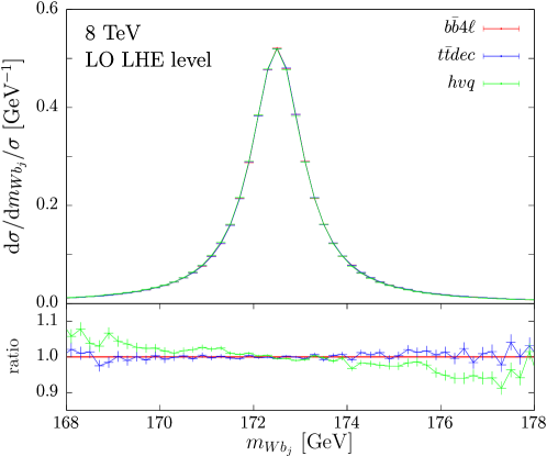
Figure 11.1: ${d\sigma}/{dm_{Wb_{j}}}$ distribution at LO obtained with $b\bar{b}4\ell$ (red), $t\bar{t}dec$ (blue) and $hvq$ (green), normalized to 1 in the displayed range. In the bottom panel the ratio with the $b\bar{b}4\ell$ prediction is shown.

This difference between the $hvq$ and the other two generators is due to the different description of how off-shell effects. The $b\bar{b}4\ell$ and $t\bar{t}dec$ generators are guaranteed to yield the correct top-virtuality distribution at the NLO and LO level, respectively. This is not the case for the $hvq$ generator, where the resonance structure is recovered by a reweighting procedure that does not guarantee LO accuracy.

We now investigate the impact of the POWHEG hardest emission(s) on the LO distributions. In Fig. 11.2 we compare $m_{Wb_{j}}$, normalized to 1 in the displayed range, at LO and NLO accuracy using the $hvq$ (left panel) and the $b\bar{b}4\ell$ (right panel) generators. Since the $hvq$ generator implements NLO corrections only in the production process, the $m_{Wb_{j}}$ distribution is not significantly modified when moving from the LO to the NLO prediction. On the other hand, the $b\bar{b}4\ell$ generator includes radiative corrections also to the decay process. Thus, when comparing the NLO and the LO curves, large differences below the peak region, that can be easily interpreted as due to radiation outside the $b$-jet cone, arise.

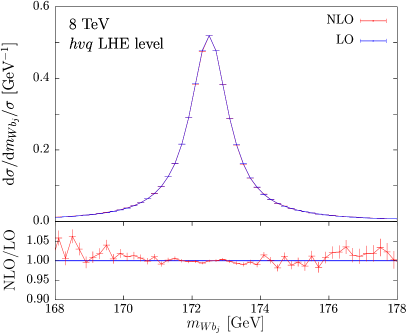
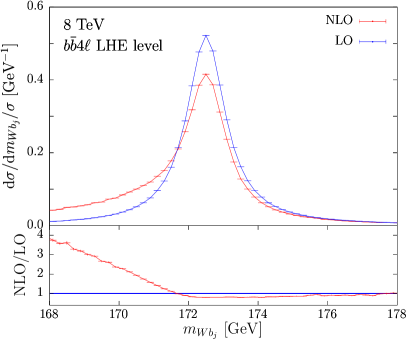
Figure 11.2: ${d\sigma}/{dm_{Wb_{j}}}$ distribution at LO (blue) and at NLO (red) obtained with the $hvq$ (left) and $b\bar{b}4\ell$ (right) generator, normalized to 1 in the displayed range. In the bottom panel the ratio with the LO prediction is shown.

The $t\bar{t}dec$ generator enables us to specify whether NLO accuracy is required both in production and decay (default behaviour), or just in production (by using the nlowhich 1 option). A graphical display of both options is given in Fig. 11.3. As we have already seen, NLO corrections in production leads to a roughly constant $K$-factor, while radiation from top decay affects the shape of the distribution.

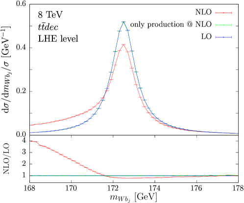
Figure 11.3: ${d\sigma}/{dm_{Wb_{j}}}$ distribution with NLO accuracy in production and decay (red), only in production (green) and with LO accuracy (blue) obtained with the $t\bar{t}dec$ generator, normalized to 1 in the displayed range. In the bottom panel the ratio with the LO prediction is shown.

11.2 Shower effects

We now investigate how the PS, that provides radiations beyond the hardest one, affect the shape of the $m_{Wb_{j}}$ distributions.

In Fig. 11.4 we can see the impact of the PS provided by Pythia8.2 (red) and by Herwig7.1 (blue) on the $hvq$ (left) and $b\bar{b}4\ell$ (right) generators. In $hvq$, we notice a large effect in the low tail of the distribution, since radiation in decay is fully generated by the shower. Conversely for $b\bar{b}4\ell$ we get smaller shower corrections, since the hardest radiation in decay is already included at the LHE level. In both cases, we see an enhancement in the region above the peak. This is attributed to shower radiation that is captured by the $b$-jet cone.

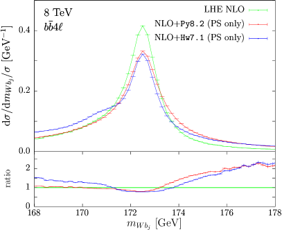
Figure 11.4: ${d\sigma}/{dm_{Wb_{j}}}$ distribution obtained with $hvq$ (left pane) and $b\bar{b}4\ell$ (right pane) at the NLO LHE level (green), and at NLO+shower (in red Pythia8.2 and in blue Herwig7.1), normalized to 1 in the displayed range. In the bottom panel the ratio with the NLO LHE is shown.

We observe that, after shower, the $hvq$ result becomes qualitatively very similar to the $b\bar{b}4\ell$ one, as shown in Fig. 11.5.

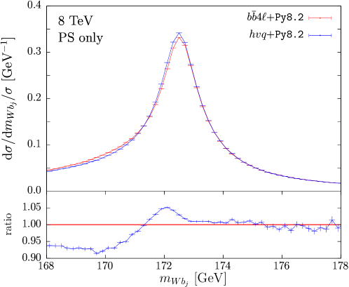
Figure 11.5: ${d\sigma}/{dm_{Wb_{j}}}$ distribution, normalized to 1 in the displayed range, obtained with $b\bar{b}4\ell$ (red) and $hvq$ (blue) at the NLO+PS level using Pythia8.2.

The inclusion of the shower in $t\bar{t}dec$ leads to effects similar to those observed in $b\bar{b}4\ell$.

11.3 Hadronization and underlying events

The effect of hadronization and multi-parton interactions (MPI), as modelled by Pythia8.2 and Herwig7.1, when interfaced to the $hvq$ generator, is showed in Fig. 11.6.

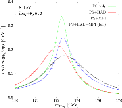
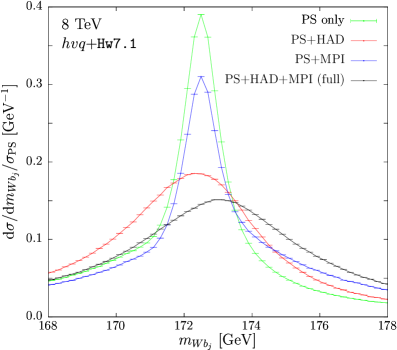
Figure 11.6: ${d\sigma}/{dm_{Wb_{j}}}$ distribution obtained with $hvq$ interfaced with Pythia8.2 (left panel) and Herwig7.1 (right panel). In green, the NLO+PS results; in red, hadronization effects are included; in blue, NLO+PS with multi-parton interactions (MPI); and in black, with hadronization and MPI effects. The curves are normalized using the NLO+PS cross section in the displayed range.

The hadronization (red) has a large impact on the final distributions. It widens the peak for both generators. However, in the Herwig7.1 case, we also observe a clear enhancement of the high mass region, that is not as evident in the Pythia8.2 case. The MPI (blue), that generate particles that can deposit in the $b$-jet cone, raise the tail of the distributions above the peak. In the combined effect of hadronization and MPI (black), Herwig7.1 has a wider peak. On the other hand, the high tail enhancement seems similar in the two generators.

The impact of the several components we have analysed, i.e. radiative corrections, the hadronization and the MPI, strongly depend on the jet-radius parameter $R$. By increasing (or decreasing) $R$, the peak position is shifted to the left (or right) as it is shown in Fig. 11.7.

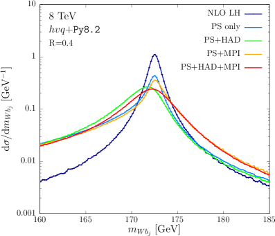
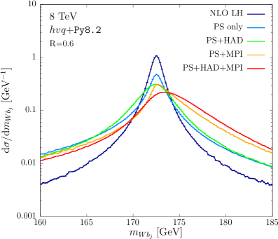
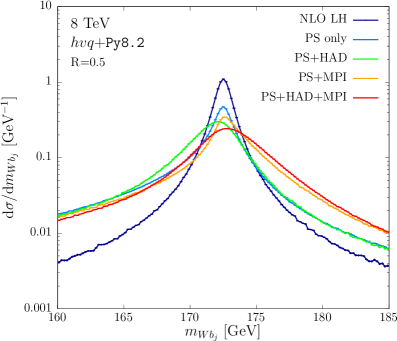
Figure 11.7: ${d\sigma}/{dm_{Wb_{j}}}$ distribution obtained with $hvq$ interfaced with Pythia8.2 for $R=0.4$ (upper-left), $R=0.5$ (down) and $R=0.6$ (upper-right). In blue, the NLO result (LH level); in azure, the PS is included; in green, the PS and the hadronization are included; in orange, the PS and the MPI are included; in red, the full results including PS, hadronization and the underlying event.

Furthermore, as we will see in Chap. 12, differences in the implementation of radiation from the resonances, the hadronization model and the underlying events can also shift the peak, leading eventually to a displacement of the extracted top mass, that should be carefully assessed for a sound estimate of the top-quark mass theoretical uncertainty.

Chapter 12 Reconstructed-top mass distribution

The peak of the reconstructed mass $m_{Wb_{j}}$, defined in Sec. 10.1, is a representative of all the direct measurement methods. To simplify our analysis, we assume we can distinguish between the $b$ and the $\bar{b}$ flavoured jets and that we can fully reconstruct the neutrinos momenta together with their sign. Our approach is very crude but it enables us to focus on theoretical issues rather then experimental ones. Indeed, if we find differences in the extracted mass using our ideal $m_{Wb_{j}}$ observable, we would be forced to conclude that there is an irreducible theoretical error (i.e. an error that cannot be reduced by increasing the experimental accuracy) on the mass measurement.

In order to mimic the experimental systematics, we introduce a Gaussian smearing to the $m_{Wb_{j}}$ distributions. If differences among the generators are found in this latter case, the problem is less severe and may be reduced once experimental resolution is improved.

However, we need to remark that also “irreducible” errors (according to the definition given above) may be reduced in practice. This is the case if one of the generators at hand does not fit satisfactorily measurable distributions related to top production. If we change the allowed range for the parameters of the generator in order to reproduce the data fairly. This procedure can reduce the error associated with top-quark mass measurements.

In Sec. 12.1 we describe the procedure for the extraction of the reconstructed-top mass peak, for both the ideal $m_{Wb_{j}}$ distribution and the smeared one. In Sec. 12.2 we will compare the three POWHEG BOX generators for $t\bar{t}$ production interfaced to Pythia8.2. Scale and PDF variations are also taken into account, together with $\alpha_{\mathchoice{\displaystyle}{\scriptstyle}{\scriptscriptstyle}{\scriptscriptstyle}\rm S}$ variations to investigate the sensitivity to the intensity of radiation from the $b$ quark. In Sec. 12.3 we investigate the differences between the Pythia8.2 and Herwig7.1 predictions and the various alternative settings that the Herwig7.1 program offers.

12.1 $\boldsymbol{m_{Wb_{j}}^{\max}{}}$ extraction

We first fit the $m_{Wb_{j}}$ distribution around the peak region. We call $Y(m_{Wb_{j}})$ the histogram of our distribution, and $y(m_{Wb_{j}},\{a\})$ our fitting functional form, where $\{a\}$ represent the fitting parameters

$$y(m_{Wb_{j}},\{a\})=\frac{a_{2}[1+a_{4}(m_{Wb_{j}}-a_{1})]}{(m_{Wb_{j}}-a_{1})^{2}+a_{3}^{2}}+a_{5}\,.$$ (12.1)

To extract the parameters $\{a\}$ we proceed as follows:

• We find the bin with the highest value, and assign its center to the variable $m_{Wb_{j}}^{\max}$.

• We find all surrounding bins whose value is not less than $Y(m_{Wb_{j}}^{\max})/2$. We assign to the variable $\Delta$ the range covered by these bins divided by two.

• We minimize the $\chi^{2}$ computed from the difference of the integral of $y(m_{Wb_{j}},\{a\})$ in each bin, divided by the bin size, with respect to $Y(m_{Wb_{j}})$, choosing as a range all bins that overlap with the segment $[m_{Wb_{j}}^{\max}-\Delta,m_{Wb_{j}}^{\max}+\Delta]$.

• From the fitted function we extract the maximum position and assign it to $m_{Wb_{j}}^{\max}$.

• If the reduced $\chi^{2}$ of the fit is less than 2, we keep this result. If not, we replace $\Delta\to 0.95\times\Delta$ and repeat the operation until this condition is met.

Once the parameters $\{a\}$ are determined, the extracted peak position $m_{Wb_{j}}^{\max}$ is found by solving

$$\frac{d\,y(m_{Wb_{j}},\{a\})}{dm_{Wb_{j}}}\Big{|}_{m_{Wb_{j}}=\,m_{Wb_{j}}^{\max}}=0\,.$$ (12.2)

Its error is derived by propagating the errors of the parameters $\{a\}$ extracted using our fitting procedures, in the expression of the peak. This procedure is applied to both the ideal $m_{Wb_{j}}$ distribution and the smeared one.

The histogram of the smeared distribution $Y_{\rm s}(m_{Wb_{j}})$ is obtained convoluting $Y(m_{Wb_{j}})$ with a Gaussian of width $\sigma=15$ GeV (that is the typical experimental resolution on the reconstructed top mass)

$$Y(m_{Wb_{j}})=\mathcal{N}\sum_{m_{i}}\Delta m_{i}\;y(m_{i})\exp\left(-\frac{(m_{Wb_{j}}-m_{i})^{2}}{2\sigma^{2}}\right)\,,$$ (12.3)

where $m_{i}$ is the central value of the $i^{\rm th}$ bin and $\Delta m_{i}$ its width. $\mathcal{N}$ is a normalization constant.

The $B$ coefficient of eq. (10.8) that links $m_{Wb_{j}}^{\max}$ and $m_{t}$ is found performing a linear fit for the three values of $m_{t}=$169.5 GeV, 172.5 GeV, 175.5 GeV. Since $m_{Wb_{j}}$ is the mass of the reconstructed top, we expect $B\approx 1$ for the $m_{Wb_{j}}^{\max}$ observable.

The values for the $B$ coefficients that we have obtained with the three generators showered with Pythia8.2 are collected in Tab. 12.1, and confirm our expectation.

	$B$, no smearing	$B$, smearing
$hvq$	$\phantom{\Big{|}}1.002\pm 0.002$	$0.949\pm 0.001$
$t\bar{t}dec$	$\phantom{\Big{|}}1.000\pm 0.002$	$0.957\pm 0.001$
$b\bar{b}4\ell$	$\phantom{\Big{|}}1.008\pm 0.002$	$0.958\pm 0.001$

Table 12.1: Values for the $B$ coefficients of eq. (10.8) for the $m_{Wb_{j}}$ peak position, for the non-smeared and smeared distributions (see Sec. 12.2 for details), obtained with the $hvq$, $t\bar{t}dec$ and $b\bar{b}4\ell$ generators showered with Pythia8.2.

Thus, we can safely assume

$$\Delta m_{t}=-\Delta m_{Wb_{j}}^{\max}{}.$$ (12.4)

12.2 Comparison among different NLO+PS generators

We begin by showing comparisons of our three generators, interfaced with Pythia8.2, for our reference top-mass value of 172.5 GeV.

The $m_{Wb_{j}}$ distributions of the $b\bar{b}4\ell$ and $t\bar{t}dec$ generators are compared in Fig. 12.1, before (left) and after (right) applying the Gaussian smearing.

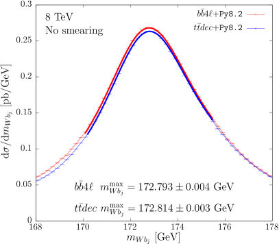
Figure 12.1: ${d\sigma}/{dm_{Wb_{j}}}$ distribution obtained with the $b\bar{b}4\ell$ and $t\bar{t}dec$ generators interfaced with Pythia8.2, for $m_{t}=172.5$ GeV, before (left) and after (right) applying the Gaussian smearing.

In the left plot we see that the two generators yield a very similar shape and the results concerning $m_{Wb_{j}}$ are very similar. This is an indication that interference effects in radiation and other off-shell effects, that are included in $b\bar{b}4\ell$ but not in $t\bar{t}dec$, have a very minor impact on the peak position, at least if we consider a measurement with an ideal resolution. The results obtained applying a 15 GeV smearing on the distribution are shown in the right plot of Fig. 12.1. The smearing procedure correlates points near the peak together with the tails of the $m_{Wb_{j}}$ distribution, increasing the impact on $m_{Wb_{j}}^{\max}$ of the region away from the peak, where there are larger differences between the two generators. This leads to a difference in the peak position of $140$ MeV.

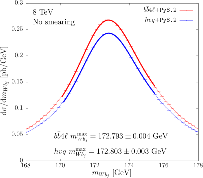
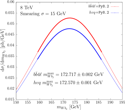
Figure 12.2: ${d\sigma}/{dm_{Wb_{j}}}$ distribution obtained with the $b\bar{b}4\ell$ and $hvq$ generators interfaced with Pythia8.2, for $m_{t}=172.5$ GeV, before (left) and after (right) applying the Gaussian smearing.

In Figs. 12.2 we compare the $b\bar{b}4\ell$ and the $hvq$ generators. We see a negligible difference in the peak position in the non-smeared case, while, in the smeared case, the $hvq$ generator differs from $b\bar{b}4\ell$ by $-147$ MeV, similar in magnitude to the case of $t\bar{t}dec$, but with opposite sign.

Our findings are summarized in Tab. 12.2, where we also include results obtained at the shower level, i.e.  without the inclusion of the underlying event and of the hadronization.

	PS only		— full
	— No smearing	15 GeV smearing	— No smearing	15 GeV smearing
— $b\bar{b}4\ell$	$172.522\pm 0.002$ GeV	$171.403\pm 0.002$ GeV	$172.793\pm 0.004$ GeV	$172.717\pm 0.002$ GeV
—$t\bar{t}dec$ ${}-$ $b\bar{b}4\ell$	$-18\pm 2$ MeV	$+191\pm 2$ MeV	$+21\pm 6$ MeV	$+140\pm 2$ MeV
—$hvq$ ${}-$ $b\bar{b}4\ell$	$-24\pm 2$ MeV	$-89\pm 2$ MeV	$+10\pm 6$ MeV	$-147\pm 2$ MeV

Table 12.2: Differences in the $m_{Wb_{j}}{}$ peak position for $m_{t}$=172.5 GeV for $t\bar{t}dec$ and $hvq$ with respect to $b\bar{b}4\ell$, showered with Pythia8.2, at the NLO+PS level and at the full hadron level.

We notice that $hvq$, even if it does not implement NLO corrections in top decay, yields to results similar to those of the most accurate $b\bar{b}4\ell$ generator. This is due to the inclusion of matrix-element corrections (MEC) in top decay by the Pythia8.2 PS. MEC are indeed equivalent, up to an irrelevant normalization factor, to next-to-leading order corrections in decay. This observation is confirmed by examining Tab. 12.3, where predictions obtained with and without MEC are compared.

	— No smearing		15 GeV smearing
	— MEC	MEC ${}-$ no MEC	MEC	MEC ${}-$ no MEC
—$b\bar{b}4\ell$	$172.793\pm 0.004$ GeV	$-12\pm 6$ MeV	$172.717\pm 0.002$ GeV	$+55\pm 2$ MeV
—$t\bar{t}dec$	$172.814\pm 0.003$ GeV	$-4\pm 5$ MeV	$172.857\pm 0.001$ GeV	$-26\pm 2$ MeV
—$hvq$	$172.803\pm 0.003$ GeV	$+61\pm 5$ MeV	$172.570\pm 0.001$ GeV	$+916\pm 2$ MeV

Table 12.3: $m_{Wb_{j}}{}$ peak position for $m_{t}$=172.5 GeV obtained with the three different generators, showered with Pythia8.2+MEC (default). We also show the differences between Pythia8.2+MEC and Pythia8.2 without MEC.

When MEC are not included, the peak position in the smeared distribution provided by the $hvq$ generator receives a considerable shift, near 1 GeV. On the other hand, the $b\bar{b}4\ell$ and $t\bar{t}dec$ generators, that already include the hardest emission off $b$ quarks, display a reduced sensitivity on the MEC. This leads to the conclusion that the MEC in Pythia8.2 do a decent job in simulating top decay as far as the $m_{Wb_{j}}$ distribution is concerned. The remaining uncertainty of roughly $140$ MeV in the case of both $hvq$ and $t\bar{t}dec$ generators, pulling in opposite directions, is likely to be due to the approximate treatment of off-shell effects.

12.2.1 Matching uncertainties

The FSREmission veto procedure described in Appendix E.3.2 represents the most accurate way to perform the vetoed shower on the POWHEG BOX generated events interfaced with the Pythia8.2, because it uses the POWHEG definition of transverse momentum rather than the Pythia8.2 one.

There is also an alternative, the ScaleResonance procedure, always described in Appendix E.3.2, where the scale of the POWHEG emissions from the $t$ and the $\bar{t}$ are set as initial scales for the showers evolutions. The ScaleResonance procedure can introduce a mismatch that we take as an indication of the size of the matching uncertainties. The extracted peak position for the $b\bar{b}4\ell$ and $t\bar{t}dec$ with the two matching procedures are summarized in Tab. 12.4.

	— No smearing		15 GeV smearing
	— SR	SR ${}{-}$ FSR	— SR	SR ${}{-}$ FSR
—$b\bar{b}4\ell$	$172.816\pm 0.004$ GeV	$+23\pm 6$ MeV	$172.737\pm 0.002$ GeV	$20\pm 2$ MeV
—$t\bar{t}dec$	$172.812\pm 0.004$ GeV	$-1\pm 5$ MeV	$172.878\pm 0.001$ GeV	$21\pm 2$ MeV

Table 12.4: $m_{Wb_{j}}{}$ peak position for $m_{t}$=172.5 GeV obtained with the $b\bar{b}4\ell$ and $t\bar{t}dec$ generators, showered with Pythia8.2, for the ScaleResonance (SR) veto procedure. The differences with FSREmission (FSR), that is our default, are also shown.

We can see that these differences are roughly 20 MeV in $b\bar{b}4\ell$ for both the no-smearing and smearing case, and in $t\bar{t}dec$ they are a few MeV for the no-smearing case, and 20 MeV with smearing.

This is due to the fact that the first emissions of the decayed top has already a small transverse momentum and in the collinear limit the POWHEG and the Pythia8.2 definitions of $p_{\perp}$ are equivalent.

We can also compare the default behaviour for dealing with radiation in the production process with the results obtained with the PowhegHooks veto machinery, that is activated with the setting

POWHEG:veto = 1.

The results are shown in Tab. 12.5.

— PowhegHooks ${}{-}$ no PowhegHooks [MeV]
— observable	$b\bar{b}4\ell$	$t\bar{t}dec$	$hvq$
$\phantom{\Big{|}}m_{Wb_{j}}^{\max}$ no smearing	$35\pm 6$	$18\pm 5$	$17\pm 5$
$\phantom{\Big{|}}m_{Wb_{j}}^{\max}$ smearing	$77\pm 2$	$78\pm 2$	$71\pm 2$

Table 12.5: Differences between the $m_{Wb_{j}}^{\max}$ predictions obtained using the POWHEG:veto = 1 and the POWHEG:veto = 0 settings for the three generators interfaced with Pythia8.2.

A slightly increased dependence on the veto procedure is found concerning radiation in the production process, since it is in general much more harder than the radiation in production and thus the two $p_{\perp}$ definitions may differ. However, we notice that even for the smeared mass distribution the differences between the $m_{Wb_{j}}^{\max}{}$ obtained with PowhegHooks and the default ones are rather small and equivalent for all the NLO generators. Thus, our choice of not using the PowhegHooks settings as default does not alter the comparison among the three codes.

12.2.2 Scale, PDF and strong-coupling variations

	— No smearing				15 GeV smearing
	— $\%$ ${}-{}$ $b\bar{b}4\ell$	$(\mu_{\mathchoice{\displaystyle}{\scriptstyle}{\scriptscriptstyle}{\scriptscriptstyle}\mathrm{R}},\mu_{\mathchoice{\displaystyle}{\scriptstyle}{\scriptscriptstyle}{\scriptscriptstyle}\mathrm{F}})$	PDF	$\alpha_{\mathchoice{\displaystyle}{\scriptstyle}{\scriptscriptstyle}{\scriptscriptstyle}\rm S}$	% ${}-{}$ $b\bar{b}4\ell$	$(\mu_{\mathchoice{\displaystyle}{\scriptstyle}{\scriptscriptstyle}{\scriptscriptstyle}\mathrm{R}},\mu_{\mathchoice{\displaystyle}{\scriptstyle}{\scriptscriptstyle}{\scriptscriptstyle}\mathrm{F}})$	PDF	$\alpha_{\mathchoice{\displaystyle}{\scriptstyle}{\scriptscriptstyle}{\scriptscriptstyle}\rm S}$
—$b\bar{b}4\ell$	$+0$ MeV	${}_{-17}^{+26}$ MeV	-	$\pm 8$ MeV	$+0$ MeV	${}_{-53}^{+86}$ MeV	-	$\pm 64$ MeV
—$t\bar{t}dec$	$+21$ MeV	${}_{-10}^{+2}$ MeV	-	$\pm 8$ MeV	$+140$ MeV	${}_{-6}^{+6}$ MeV	-	$\pm 54$ MeV
—$hvq$	$+10$ MeV	${}_{-6}^{+2}$ MeV	$\pm 3$ MeV	$\pm 2$ MeV	$-147$ MeV	${}_{-7}^{+7}$ MeV	$\pm 5$ MeV	$\pm 9$ MeV

Table 12.6: Theoretical uncertainties associated with the $m_{Wb_{j}}{}$ peak position extraction for $m_{t}$=172.5 GeV for the three different generators, showered with Pythia8.2. The PDF uncertainty on the $b\bar{b}4\ell$ and $t\bar{t}dec$ generators is assumed to be equal to the $hvq$ one, as explained in Chap. 10.

In Tab. 12.6 we summarize the uncertainties due to scale, PDF and strong-coupling variations, connected with the extraction of the $m_{Wb_{j}}$ peak position, for the input mass $m_{t}=172.5$ GeV, for all the generators showered with Pythia8.2.

The upper (lower) error due to scale variation reported in the table is obtained by taking the maximum (minimum) position of the $m_{Wb_{j}}$ peak for each of the seven scales choices of eq. (10.5), minus the one obtained for the central scale.

In the PDF case, as discussed in Chap. 10, we compute the PDF uncertainties only for the $hvq$ generator, and assume that they are the same for $b\bar{b}4\ell$ and $t\bar{t}dec$.

We consider a symmetrized strong-coupling dependence uncertainty, whose expression is given by

$$\Delta{m_{Wb_{j}}\left(\alpha_{\mathchoice{\displaystyle}{\scriptstyle}{\scriptscriptstyle}{\scriptscriptstyle}\rm S}(m_{\mathchoice{\displaystyle}{\scriptstyle}{\scriptscriptstyle}{\scriptscriptstyle}Z})\right)}=\pm\frac{\left|m_{Wb_{j}}\left(\alpha_{\mathchoice{\displaystyle}{\scriptstyle}{\scriptscriptstyle}{\scriptscriptstyle}\rm S}(m_{\mathchoice{\displaystyle}{\scriptstyle}{\scriptscriptstyle}{\scriptscriptstyle}Z})=0.115\right)-m_{Wb_{j}}\left(\alpha_{\mathchoice{\displaystyle}{\scriptstyle}{\scriptscriptstyle}{\scriptscriptstyle}\rm S}(m_{\mathchoice{\displaystyle}{\scriptstyle}{\scriptscriptstyle}{\scriptscriptstyle}Z})=0.121\right)\right|}{2}\,.$$ (12.5)

We stress that these variations have only an indicative meaning. In a realistic analysis, experimental constraints may reduce these uncertainties. We also stress that these are not the only theoretical uncertainties. Others may be obtained by varying MC parameters. Here we focus specifically on those uncertainties that are associated with the NLO+PS generators.

As we have already discussed, the use of the $hvq$ and the $t\bar{t}dec$ generators would lead to a negligible bias in the $m_{Wb_{j}}$ distribution if we were able to measure it without any resolution effects. However, if we introduce a smearing to mimic them, the description of the region away from the peak plays an important role, and the $hvq$ and $t\bar{t}dec$ generators yield predictions for the mass peak position that are shifted by roughly $140$ MeV in the downward and upward direction respectively with respect to $b\bar{b}4\ell$.

We also notice that the $b\bar{b}4\ell$ generator is the most affected by theoretical uncertainties. In particular, the $t\bar{t}dec$ and $hvq$ generators have an unrealistically small scale dependence of the peak shape, due to the way in which off-shell effects are approximately described. The $t\bar{t}dec$ generator displays a non-negligible sensitivity only to the strong-coupling constant. The theoretical errors that we have studied here lead to very small effects for the $hvq$ generator, since it does not include radiative corrections in the top decay. On the other hand, the $hvq$ generator is bound to be more sensitive to variation of parameters in Pythia8.2, that in this case fully controls the radiation from the $b$ quark.

12.2.3 Radius dependence

In this section we investigate the stability of the previous results with respect to the choice of the jet radius. The results are summarized in Tab. 12.7.

	— $R=0.4$		— $R=0.5$		— $R=0.6$
	— No smearing	15 GeV smearing	— No smearing	15 GeV smearing	— No smearing	15 GeV smearing
— $b\bar{b}4\ell$ [GeV]	$172.156\pm 0.004$	$171.018\pm 0.002$	$172.793\pm 0.004$	$172.717\pm 0.002$	$173.436\pm 0.005$	$174.378\pm 0.002$
—$t\bar{t}dec$ ${}-$ $b\bar{b}4\ell$	$+35\pm 5$ MeV	$+195\pm 2$ MeV	$+21\pm 6$ MeV	$+140\pm 2$ MeV	$+1\pm 7$ MeV	$+97\pm 2$ MeV
—$hvq$ ${}-$ $b\bar{b}4\ell$	$+47\pm 5$ MeV	$-113\pm 2$ MeV	$+10\pm 6$ MeV	$-147\pm 2$ MeV	$-7\pm 6$ MeV	$-174\pm 2$ MeV

Table 12.7: $m_{Wb_{j}}$ peak position obtained with the $b\bar{b}4\ell$ generator for three choices of the jet radius. The differences with the $t\bar{t}dec$ and the $hvq$ generators are also shown.

For the distributions without smearing, the differences between the three generators are small and decrease as $R$ increases. For the smeared distributions, the differences between $t\bar{t}dec$ and $b\bar{b}4\ell$ decrease as the radius increases, while the difference between the $hvq$ and the $b\bar{b}4\ell$ generator increases.

The small differences in the $R$ dependence among the three generators in the non-smeared cases can be understood if we consider that differences in the $b$ radiation do not affect much the peak position in the non-smeared distribution, but rather they affect the strength of the tail on the left side of the peak. On the other hand, the peak position is affected by radiation in production and by the underlying-event structure, that is very similar in the three generators.

It should be noticed that the difference between the displacements of the $t\bar{t}dec$ and $hvq$ with respect to $b\bar{b}4\ell$ is less than $55$ MeV and $34$ MeV, respectively, below the current statistical precision of top-mass measurements. Thus, the good agreement found among the three generators persists also for different $R$ values.

12.3 Comparison with Herwig7.1

In order to assess uncertainties due to the shower Monte Carlo (SMC) program, in this section we compare the results obtained using Herwig7.1 and Pythia8.2.

	— No smearing		15 GeV smearing
	— Hw7.1	Py8.2 ${}-$ Hw7.1	— Hw7.1	Py8.2 ${}-$ Hw7.1
—$b\bar{b}4\ell$	$172.727\pm 0.005$ GeV	$+66\pm 7$ MeV	$171.626\pm 0.002$ GeV	$+1091\pm 2$ MeV
—$t\bar{t}dec$	$172.775\pm 0.004$ GeV	$+39\pm 5$ MeV	$171.678\pm 0.001$ GeV	$+1179\pm 2$ MeV
—$hvq$	$173.038\pm 0.004$ GeV	$-235\pm 5$ MeV	$172.319\pm 0.001$ GeV	$+251\pm 2$ MeV

Table 12.8: $m_{Wb_{j}}{}$ peak position for $m_{t}$=172.5 GeV obtained with the three different generators, showered with Herwig7.1 (Hw7.1). The differences with Pythia8.2 (Py8.2) are also shown.

In Tab. 12.8 we compare the $m_{Wb_{j}}$ peak position extracted for the input mass $m_{t}=172.5$ GeV using the three generators showered with Pythia8.2 and Herwig7.1. For the $hvq$ generator, the differences are of the order of $240$ MeV for both the smeared and non-smeared case, but with opposite signs. In the smeared case, both the $t\bar{t}dec$ and $b\bar{b}4\ell$ generators yield much larger differences, of more than 1 GeV.

In Tab. 12.9 we report the differences between the Herwig7.1 and Pythia8.2 predictions for all the generators, at the NLO+PS level and at the full hadron level.

	Pythia8.2 ${}-$ Herwig7.1
	PS only		— full
	— No smearing	15 GeV smearing	— No smearing	15 GeV smearing
—$b\bar{b}4\ell$	$+10\pm 2$ MeV	$+984\pm 2$ MeV	$+66\pm 7$ MeV	$+1091\pm 2$ MeV
—$t\bar{t}dec$	$+5\pm 2$ MeV	$+1083\pm 2$ MeV	$+39\pm 5$ MeV	$+1179\pm 2$ MeV
—$hvq$	$-0\pm 2$ MeV	$+113\pm 2$ MeV	$-235\pm 5$ MeV	$+251\pm 2$ MeV

Table 12.9: Differences between Pythia8.2 and Herwig7.1 in the extracted $m_{Wb_{j}}{}$ peak position for $m_{t}$=172.5 GeV obtained with the three different generators, at the NLO+PS level (PS only) and including also the underlying events, the multi-parton interactions and the hadronization (full).

We notice that at the NLO+PS level and without smearing, the differences between the two parton-shower programs are negligible. For the smeared distributions, at both the NLO+PS and full level, the differences are roughly 1 GeV for the $b\bar{b}4\ell$ and the $t\bar{t}dec$ generator. For $hvq$ the differences are considerably smaller, although not quite negligible.

The origin of these large differences is better understood by looking at the differential cross sections plotted in Figs. 12.3 and 12.4.

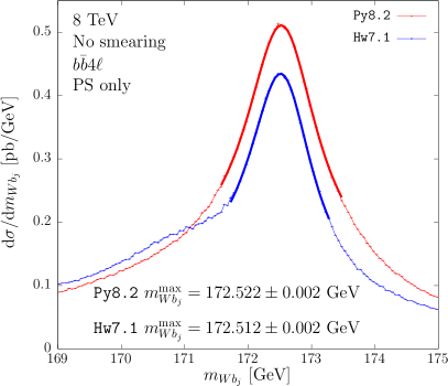
Figure 12.3: ${d\sigma}/{dm_{Wb_{j}}}$ distribution obtained by showering the $b\bar{b}4\ell$ results with Pythia8.2 and Herwig7.1, at parton-shower level (left) and with hadronization and underlying events (right).

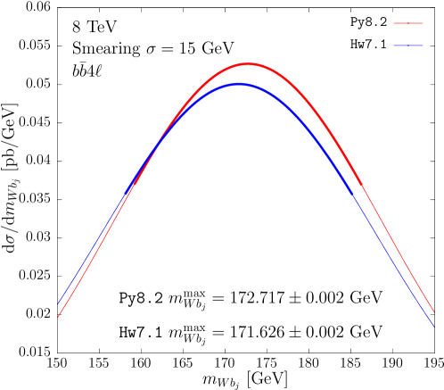
Figure 12.4: Smeared ${d\sigma}/{dm_{Wb_{j}}}$ distribution obtained by matching the $b\bar{b}4\ell$ generator with Pythia8.2 and Herwig7.1.

In Fig. 12.3 we plot the results for the non-smeared case, at the NLO+PS level (left) and at the full hadron level (right): while the peak position is nearly the same for both Pythia8.2 and Herwig7.1, the shape of the curves is very different around the peak, leading to a different mass peak position when smearing is applied, as displayed in Fig. 12.4. We notice that in this last case we see a difference in shape also after smearing. This suggests that at least one of the two generators may not describe the data fairly.

Since we observe such large differences in the value of $m_{Wb_{j}}^{\max}$ in Herwig7.1 and Pythia8.2, we have also studied whether sizeable differences are also present in the $m_{Wb_{j}}^{\max}$ dependence upon the jet radius $R$. The results are shown in Tab. 12.10, and displayed in Fig. 12.5.

	— Pythia8.2 ${}-$ Herwig7.1
	— $R=0.4$		— $R=0.5$		— $R=0.6$
	— No smearing	15 GeV smearing	— No smearing	15 GeV smearing	— No smearing	15 GeV smearing
—$b\bar{b}4\ell$	$-98\pm 7$ MeV	$+830\pm 2$ MeV	$+66\pm 7$ MeV	$+1091\pm 2$ MeV	$+253\pm 8$ MeV	$+1267\pm 2$ MeV
—$t\bar{t}dec$	$-100\pm 5$ MeV	$+979\pm 2$ MeV	$+39\pm 5$ MeV	$+1179\pm 2$ MeV	$+210\pm 6$ MeV	$+1314\pm 2$ MeV
—$hvq$	$-370\pm 5$ MeV	$+73\pm 2$ MeV	$-235\pm 5$ MeV	$+251\pm 2$ MeV	$-31\pm 6$ MeV	$+389\pm 2$ MeV

Table 12.10: Differences in the $m_{Wb_{j}}$ peak position obtained matching the three generators with Pythia8.2 and Herwig7.1, for three choices of the jet radius.

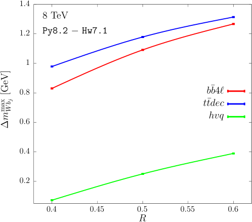
Figure 12.5: Differences of $m_{Wb_{j}}^{\max}$ between the Pythia8.2 and the Herwig7.1 showers, for the three generators, as a function of the jet radius.

In the case of the $b\bar{b}4\ell$ generator, the difference between Pythia8.2 and Herwig7.1 goes from $830$ to $1267$ MeV. Thus, assuming for instance that Pythia8.2 fits the data perfectly, i.e. that it extracts the same value of the mass by fitting the $m_{Wb_{j}}^{\max}$ values obtained with the three different values of $R$, Herwig7.1 would extract at $R=0.6$ a mass value that is larger by $437$ MeV from the one extracted at $R=0.4$. We stress that the differences in the $R$ behaviour of $m_{Wb_{j}}^{\max}$ may have the same origin as the difference in the reconstructed mass value, since both effects may be related to the amount of energy that enters the jet cone, and it is not unlikely that, by tuning one of the two generators in such a way that they both have the same $R$ dependence, their difference in $m_{Wb_{j}}^{\max}$ would also be reduced. It is unlikely, however that this would lead to a much improved agreement, since the difference in slope is much less pronounced than the difference in absolute value.

12.3.1 Alternative settings in Herwig7.1

We have examined several variations in the Herwig7.1 settings, in order to understand whether the Herwig7.1 results are reasonably stable, or depend upon our particular settings.

12.3.1.1 MEC and POWHEG options in Herwig7.1

Herwig7.1 applies matrix-element corrections by default, but it also offers the possibility to replace the MEC with its internal POWHEG method, when available, to achieve NLO accuracy in top decays. These options are activated by the instructions

set ShowerHandler:HardEmission None

or

set ShowerHandler:HardEmission POWHEG

respectively. We have verified that, as expected, switching off the matrix-element corrections does not significantly affect the $b\bar{b}4\ell$ and $t\bar{t}dec$ results. In the case of the $hvq$ generator, we can compare the default case, where MEC is on, with the cases where POWHEG replaces MEC, and with the case where neither MEC nor POWHEG is implemented. The results are shown in Tab. 12.11.

$hvq$	— No smearing	15 GeV smearing
— MEC ${}-$ no MEC	$307\pm 6$ MeV	$1371\pm 2$ MeV
— MEC ${}-$ POWHEG	$244\pm 6$ MeV	$356\pm 2$ MeV

Table 12.11: Differences in the $m_{Wb_{j}}{}$ peak position for the $hvq$ generator showered with Herwig7.1, with MEC switched off (no MEC) or using the Herwig7.1 POWHEG option, with respect to our default setting, that has MEC switched on.

We notice that the inclusion of MEC enhances by more than 1.3 GeV the peak position of the smeared distribution. A similar result was found in Pythia8.2 (see Tab. 12.3), where the difference was slightly less than 1 GeV. The difference between the POWHEG and MEC results is much below the 1 GeV level but not negligible. This fact is hard to understand, since the POWHEG and MEC procedures should only differ by a normalization factor.

We have seen previously that the three NLO+PS generators interfaced to Pythia8.2 yield fairly consistent results for the reconstructed top mass peak. The same consistency is not found when they are interfaced to Herwig7.1. However, the best agreement is found when the internal POWHEG option for top decay is activated in Herwig7.1, as can be seen in Tab. 12.12.

	PS only		— full
	— No smearing	15 GeV smearing	— No smearing	15 GeV smearing
— $b\bar{b}4\ell$	$172.512\pm 0.002$ GeV	$170.419\pm 0.002$ GeV	$172.727\pm 0.005$ GeV	$171.626\pm 0.002$ GeV
—$t\bar{t}dec$ ${}-$ $b\bar{b}4\ell$	$-13\pm 2$ MeV	$+92\pm 2$ MeV	$+48\pm 7$ MeV	$+52\pm 2$ MeV
—$hvq$ ${}-$ $b\bar{b}4\ell$	$-14\pm 2$ MeV	$+782\pm 2$ MeV	$+311\pm 7$ MeV	$+693\pm 2$ MeV
—$hvq$+PWG ${}-$ $b\bar{b}4\ell$	$-16\pm 2$ MeV	$+479\pm 2$ MeV	$+67\pm 7$ MeV	$+337\pm 2$ MeV

Table 12.12: Differences of $hvq$ and $t\bar{t}dec$ with respect to $b\bar{b}4\ell$, all showered with Herwig7.1. The result obtained using the Herwig7.1 internal POWHEG implementation of top decay, rather than MEC, labelled as $hvq$+PWG, is also shown.

The difference between the POWHEG and MEC or POWHEG Herwig7.1 results is puzzling, since they have the same formal accuracy. We will comment about this issue later on.

12.3.1.2 Veto procedures in Herwig7.1

	— No smearing		15 GeV smearing
	— FSV	FSV ${}-$ SV	— FSV	FSV ${}-$ SV
—$b\bar{b}4\ell$	$172.776\pm 0.005$ GeV	$+49\pm 7$ MeV	$171.829\pm 0.002$ GeV	$+203\pm 2$ MeV
—$t\bar{t}dec$	$172.810\pm 0.004$ GeV	$+35\pm 6$ MeV	$171.906\pm 0.001$ GeV	$+228\pm 2$ MeV

Table 12.13: $m_{Wb_{j}}{}$ peak position for $m_{t}$=172.5 GeV for $b\bar{b}4\ell$ and $t\bar{t}dec$ showered with Herwig7.1 using the FullShowerVeto (FSV) procedure. The differences with ShowerVeto (SV), that represents our default, are also shown.

As discussed in Appendix . E.3.3, Herwig7.1 offers two different classes that implement the veto procedure: the ShowerVeto, our default one, where the veto is performed at the emission level, and the FullShowerVeto class, where the veto is performed at the end of the whole showering phase. The corresponding results are summarized in Tab. 12.13. For both the $b\bar{b}4\ell$ and the $t\bar{t}dec$ the two procedures lead to a 200 MeV difference in the peak position for the smeared distributions. The origin of such difference is not fully clear to us. In part it may be ascribed to the fact that when using the ShowerVeto class we mix two different definitions of transverse momentum (the Herwig7.1 and the POWHEG one), and in part may be due to the fact that in the FullShowerVeto class the vetoing is done on the basis of the shower structure after reshuffling has been applied.

12.3.1.3 Truncated showers

In Ref. [98] it was shown that, when interfacing a POWHEG generator to an angular-ordered shower, in order to compensate for the mismatch between the angular-ordered scale and the POWHEG hardness, that is taken equal to the relative transverse momentum in radiation, one should supply appropriate truncated showers. None of our vetoing algorithms take them into account, but it turns out that Herwig7.1 provides facilities to change the settings of the initial showering scale according to the method introduced in Ref. [99], that, in our case, are equivalent to the inclusion of truncated showers (see Appendix E.3.3). The effects this inclusion, performed with the settings of eq. (E.27), for the $b\bar{b}4\ell$ and $t\bar{t}dec$ generators are shown in Tab. 12.14.

	— No smearing		15 GeV smearing
	— TS	TS ${}-$ default	— TS	TS ${}-$ default
—$b\bar{b}4\ell$	$172.730\pm 0.005$ GeV	$+3\pm 8$ MeV	$171.496\pm 0.002$ GeV	$-130\pm 2$ MeV
—$t\bar{t}dec$	$172.786\pm 0.004$ GeV	$+12\pm 6$ MeV	$171.546\pm 0.001$ GeV	$-132\pm 2$ MeV

Table 12.14: $m_{Wb_{j}}{}$ peak position for $m_{t}$=172.5 GeV obtained with the $b\bar{b}4\ell$ and $t\bar{t}dec$ generators showered with Herwig7.1, with the settings of eq. (E.27) (labelled as TS). The differences with the default results are also shown.

As we can see, this does not introduce dramatic changes in the peak position: in fact the differences are negligible in the distributions without smearing, and are roughly $130$ MeV when smearing is applied. It should be noticed that these settings slightly increase the difference with respect to the results obtained with Pythia8.2.

Chapter 13 The energy of the $\boldsymbol{b}$ jet

In Ref. [67] it was proposed to extract $m_{t}$ using the peak of the energy spectrum of the $b$ jet. This method has been investigated by the CMS collaboration in Ref. [73], where it was found

$$m_{t}=172.29\,\pm\,1.17{\rm\,(stat)\,}\pm 2.66{\rm\,(syst)}\leavevmode\nobreak\ {\rm GeV}$$ (13.1)

At leading order, the $b$ jet consists of the $b$ quark alone, and its energy in the top rest frame, neglecting top-width effects, is fixed and given by

$$E_{b_{j}}^{\max}=\frac{m_{t}^{2}-m_{W}^{2}+m_{b}^{2}}{2\,m_{t}}\,,$$ (13.2)

i.e. the spectrum is a delta function in the energy and its value is independent from the top-production mechanism. In the laboratory frame, because of the variable boost that affects the top, the delta function is smeared into a wider distribution, but it can be shown that its peak position remains at $E_{b_{j}}^{\max}$. On the basis of this observation we are led to assume that also after the inclusion of off-shell effects, radiative and non-perturbative corrections, the relation between $E_{b_{j}}^{\max}$ and the top pole-mass $m_{t}$ should be largely insensitive to production dynamics.

We performed a study of the $E_{b_{j}}^{\max}$ observable along the same lines adopted for $m_{Wb_{j}}$ in the previous section. If the range of variations of the top mass around a given central value $m_{t,\,c}$ is small enough, a linear relation between $E_{b_{j}}^{\max}$ and the top mass must hold, so that we can write

$$E_{b_{j}}^{\max}(m_{t})=E_{b_{j}}^{\max}(m_{t,\,c})+B\,(m_{t}-m_{t,\,c})+\mathcal{O}(m_{t}-m_{t,\,c})^{2}.$$ (13.3)

It was suggested in Ref. [73] that the $E_{b_{j}}$ distribution $\mathrm{d}\sigma/\mathrm{d}E_{b_{j}}$ is better fitted in terms of $\log E_{b_{j}}$. Thus, in order to extract the peak position, we fitted the energy distribution with a fourth order polynomial

$$y=a+b(x-x^{\rm max})^{2}+c(x-x^{\rm max})^{3}+d(x-x^{\rm max})^{4}\,,$$ (13.4)

where $x=\log E_{b_{j}}$. The fitting procedure is the same employed to extract $m_{Wb_{j}}^{\max}$, that is described in Sec. 12.1

The parameter $B$ of eq. (13.3), extracted from a linear fit of the three $E_{b_{j}}^{\max}$ values corresponding to the three different values of $m_{t}$ that we have considered (see Tab. 10.1) using the $hvq$ generator showered by Pythia8.2, was found to be

$$B=0.50\pm 0.03\,,$$ (13.5)

compatible with the expected value of 0.5 from eq. (13.2).

13.1 Comparison among different NLO+PS generators

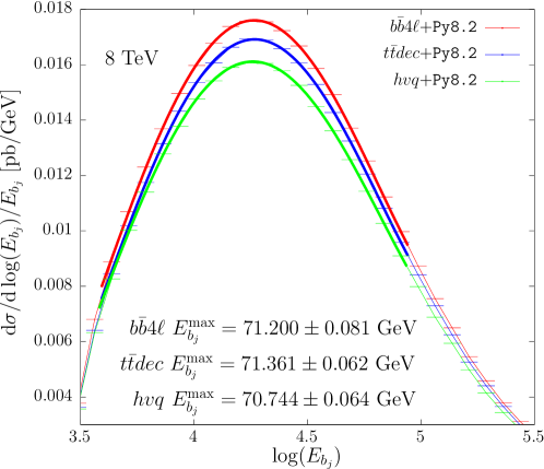
Figure 13.1: Logarithmic energy distribution obtained with the three generators interfaced to Pythia8.2, together with their polynomial fit, in the range displayed in the figure. The value of $E_{b_{j}}^{\max}$ for each generator is also reported.

In Fig. 13.1 we plot the logarithmic energy distribution for the three generators interfaced to Pythia8, together with their polynomial fit. The extracted $E_{b_{j}}$ peaks from the $b\bar{b}4\ell$ and the $t\bar{t}dec$ generators are compatible within the statistical errors. On the other hand, the $hvq$ generator yields a prediction which is roughly $460$ $\pm$ $100$ MeV smaller than the $b\bar{b}4\ell$ one. We thus observe that the jet modelling implemented by Pythia8.2 with MEC seems to yield slightly less energetic jets. An effect going in the same direction was also observed for the $m_{Wb_{j}}$ observable (see Tab. 12.6, the first column of the results with smearing), although to a smaller extent.

	MEC	MEC ${}-$ no MEC
$b\bar{b}4\ell$	$71.200\pm 0.081$ GeV	$+170\pm 115$ MeV
$t\bar{t}dec$	$71.361\pm 0.062$ GeV	$-69\pm 87$ MeV
$hvq$	$70.744\pm 0.064$ GeV	$+1937\pm 92$ MeV

Table 13.1: $E_{b_{j}}$ peak position obtained with the three generators showered with Pythia8.2. The differences between the peak positions extracted by switching on and off the matrix-element corrections are also shown.

In Tab. 13.1 we have collected the values of $E_{b_{j}}^{\max}$ computed with MEC, and the differences between the results with and without MEC. We notice that the MEC setting has little impact in the $b\bar{b}4\ell$ and $t\bar{t}dec$ cases. On the other hand, in the $hvq$ case the absence of MEC would have lead to an $E_{b_{j}}^{\max}$ value about 2 GeV smaller than with MEC. We take this as another indication that the implementation of radiation in top decay using MEC leads to results that are much closer to the NLO+PS ones.

In Tab. 13.2

	$\%$ ${}-$ $b\bar{b}4\ell$	$(\mu_{\mathchoice{\displaystyle}{\scriptstyle}{\scriptscriptstyle}{\scriptscriptstyle}\mathrm{R}},\mu_{\mathchoice{\displaystyle}{\scriptstyle}{\scriptscriptstyle}{\scriptscriptstyle}\mathrm{F}})$	PDF	$\alpha_{\mathchoice{\displaystyle}{\scriptstyle}{\scriptscriptstyle}{\scriptscriptstyle}\rm S}$	stat
$b\bar{b}4\ell$	$+0$ MeV	${}_{-15}^{+22}$ MeV	-	$\pm 35$ MeV	$\pm 81$ MeV
$t\bar{t}dec$	$+161$ MeV	${}_{-24}^{+22}$ MeV	-	$\pm 17$ MeV	$\pm 62$ MeV
$hvq$	$-456$ MeV	${}_{-47}^{+32}$ MeV	$\pm 30$ MeV	$\pm 25$ MeV	$\pm 64$ MeV

Table 13.2: Theoretical uncertainties for the $E_{b_{j}}$ peak position obtained with the three generators showered with Pythia8.2. The last column reports the statistical uncertainty of our results.

we summarize our results together with the scale, PDF and $\alpha_{\mathchoice{\displaystyle}{\scriptstyle}{\scriptscriptstyle}{\scriptscriptstyle}\rm S}$ uncertainties, that are extracted with a procedure analogous to one described for the $m_{Wb_{j}}$ observable. We also report the corresponding statistical errors of our results. We see that scale and PDF variations have negligible impact on our observable, given the small sensitivity on the production dynamics, the only important change being associated with the choice of the NLO+PS generator.

We notice that our errors on scale and PDF variations are much smaller than our statistical errors. On the other hand, these variations are performed by reweighting techniques, that, because of correlations, lead to errors in the differences that are much smaller than the error on the individual term. In view of the small size of these variations, we do not attempt to perform a better estimate of their error. On the other hand, the variation of $\alpha_{\mathchoice{\displaystyle}{\scriptstyle}{\scriptscriptstyle}{\scriptscriptstyle}\rm S}$ do not benefit from this cancellation, and are all below the statistical uncertainties.

As previously done for $m_{Wb_{j}}$, we have also investigated the dependence of the $b$-jet peak positions on the jet radius. The results are summarized in Tab. 13.3.

	$R=0.4$	$R=0.5$	$R=0.6$
$b\bar{b}4\ell$	$67.792\pm 0.089$ GeV	$71.200\pm 0.081$ GeV	$74.454\pm 0.076$ GeV
$t\bar{t}dec$ ${}-$ $b\bar{b}4\ell$	$+365\pm 110$ MeV	$+161\pm 102$ MeV	$+75\pm 97$ MeV
$hvq$ ${}-$ $b\bar{b}4\ell$	$-563\pm 110$ MeV	$-456\pm 103$ MeV	$-323\pm 97$ MeV

Table 13.3: $E_{b_{j}}$ peak position obtained with the $b\bar{b}4\ell$ generator showered with Pythia8.2, for three choices of the jet radius. The differences with the $t\bar{t}dec$ and the $hvq$ generators are also shown.

While we observe a marked change in $E_{b_{j}}^{\max}$, that grows by $3.4$ and $3.3$ GeV when going from $R=0.4$ to $0.5$ and from $0.5$ to $0.6$ respectively, $t\bar{t}dec$ and $hvq$ differ by $b\bar{b}4\ell$ by much smaller amounts. It is not clear whether such small differences could be discriminated experimentally.

According to eqs. (10.11) and (13.5), the uncertainties that affect the value of the extracted top mass are nearly twice the uncertainties on the $b$-jet energy. Considering the difference for $R=0.5$ between $hvq$ and $b\bar{b}4\ell$ in Tab. 13.3, we see that, by using $hvq$ instead of $b\bar{b}4\ell$, the extracted top mass would be roughly 900 MeV larger. This should be compared with the corresponding difference of about 150 MeV, that is shown in Tab. 12.7, for the smeared $m_{Wb_{j}}$ case. In any case, these difference are much more smaller than the statical error of 2.66 GeV quoted by CMS in Ref. [73].

As before, we have checked the sensitivity of our result to variations in the matching procedure in Pythia8.2, by studying the difference between ScaleResonance and FSREmission options. The differences turn out to be of the order of the statistical error.

13.2 Comparison with Herwig7.1

In this section, we study the dependence of our results on the shower MC program, comparing Herwig7.1 and Pythia8.2 predictions. We extract the differences in the $E_{b_{j}}^{\max}$ position for three values of the jet radius: $R=0.4$, 0.5 and 0.6. The results are summarized in Tab. 13.4, where we also show the results at the PS-only level,

	Pythia8.2 ${}-$ Herwig7.1 [MeV]
	$R=0.4$		$R=0.5$		$R=0.6$
	PS only	full	PS only	full	PS only	full
$b\bar{b}4\ell$	$+1297\pm 120$	$+1631\pm 122$	$+1666\pm 117$	$+2150\pm 114$	$+1802\pm 114$	$+2356\pm 113$
$t\bar{t}dec$	$+1786\pm 91$	$+2039\pm 91$	$+2179\pm 88$	$+2332\pm 88$	$+2121\pm 89$	$+2437\pm 87$
$hvq$	$+515\pm 94$	$+762\pm 93$	$+707\pm 90$	$+1028\pm 89$	$+779\pm 87$	$+1188\pm 86$

Table 13.4: Differences in the $E_{b_{j}}$ peak position between the Pythia8.2 and the Herwig7.1 showers applied to the three generators for three choices of the jet radius. The results at the NLO+PS level (PS only) are also shown.

and in Fig. 13.2.

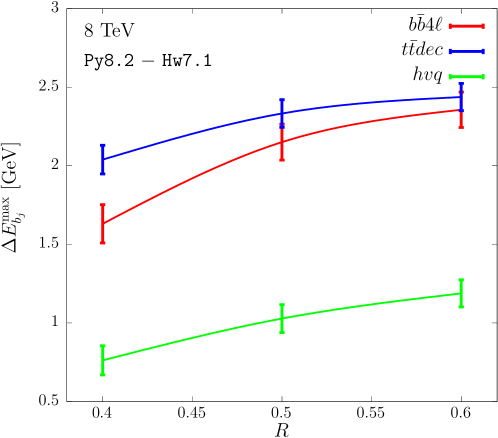
Figure 13.2: Differences of $E_{b_{j}}^{\max}$ between the Pythia8.2 and the Herwig7.1 showers, for the three generators, as a function of the jet radius.

From Tab. 13.4 we clearly see that the $b\bar{b}4\ell$ and the $t\bar{t}dec$ generators display larger discrepancies. For example, for the central value $R=0.5$, we would get $\Delta E_{b_{j}}^{\max}{}\approx 2$ GeV, that roughly corresponds to $\Delta m_{t}=-4$ GeV, much larger than the 2.66 GeV statistical error quoted in Ref. [73]. In the case of the $hvq$ generator the difference is near 1 GeV, implying that the extracted mass using $hvq$+Herwig7.1 would be 2 GeV bigger than the one obtained with $hvq$+Pythia8.2.

We find that the differences between Herwig7.1 and Pythia8.2 increases for larger jet radii. Furthermore, by looking at Fig. 13.2, we notice that the $b\bar{b}4\ell$ generator displays a different $R$ dependence, as we have already observed from Tab. 13.3. Figure 13.2 indicates that $b\bar{b}4\ell$ and $t\bar{t}dec$ are in better agreement for larger values of the jet radius. This was also observed for the peak of the $m_{Wb_{j}}$ smeared distribution (Tab. 12.7).

We notice that, as in the case of the reconstructed mass peak, the predominant contribution to the difference arise at the PS level.

As for the previous cases, we have examined the variations due to a different choice of the matching scheme in Herwig7.1, that we found to be below the 200 MeV level, and thus negligible in the present context.

Chapter 14 Leptonic observables

In this section, we investigate the extraction of the top mass from the leptonic observables introduced in Ref. [68]. This method has been recently studied by the ATLAS collaboration in Ref. [75] that finds

$$m_{t}=173.2\,\pm\,0.9{\rm\,(stat)\,}\pm\,0.8{\rm\,(syst)\,}\pm\,1.2{\rm\,(theo)}\leavevmode\nobreak\ {\rm GeV}.$$ (14.1)

Following Ref. [68], we consider the subsequent five observables

$$\begin{array}[]{l l l }O_{1}=p_{\perp}(\ell^{+}),&O_{2}=p_{\perp}(\ell^{+}\ell^{-}),&O_{3}=m(\ell^{+}\ell^{-}),\\[5.69054pt] O_{4}=E(\ell^{+}\ell^{-}),&O_{5}=p_{\perp}(\ell^{+})+p_{\perp}(\ell^{-}),&\end{array}$$

i.e. the transverse momentum of the positive charged lepton, and the transverse momentum, the invariant mass, the energy and the scalar sum of the transverse momenta of the lepton pair. We compute the average value of the first three Mellin moments for each of the above mentioned observables, $\langle(O_{i})^{j}\rangle$, with $i=1,\dots,5$ and $j=1,2,3$. We assume that, if we do not vary too much the range of the top mass, we can write the linear relation

$$\langle(O_{i})^{j}\rangle=O_{\rm c}^{(ij)}+B^{(ij)}\left[\left(m_{t}\right)^{j}-\left(m_{t,\,c}\right)^{j}\right].$$ (14.2)

For ease of notation, we will refer to $O_{\rm c}^{(ij)}$ and $B^{(ij)}$ as $O_{\rm c}$ and $B$ in the following. Their determination will be discussed later.

We choose as reference sample the one generated with $b\bar{b}4\ell$ matched with Pythia8.2, using $m_{t,\,c}=172.5$ GeV as input mass and the central choices for the PDF and scales. We indicate the values of the observables computed with this generator as ${O}^{b\bar{b}4\ell}$, and with $O_{\rm c}^{\prime}$ the values of the observable computed either with an alternative generator or with different generator settings, but using as input parameter the same reference mass. The mass value that we would extract from the events of the reference sample using the new generator is then given by

$$m_{t}^{\prime}=\left[\left(m_{t,\,c}\right)^{j}-\frac{O^{\prime}_{\rm c}-{O}^{b\bar{b}4\ell}_{\rm c}}{B}\right]^{1/j}\,.$$ (14.3)

Since all the leptonic observables are statistical-correlated among each other, we then performed a weighted average of all the results considering as covariance matrix

$$V_{\alpha\beta}=\min\left[\sigma^{2}\left(m_{t}^{(\alpha)}\right)\,,\;\sigma^{2}\left(m_{t}^{(\beta)}\right)\,,\;C_{\alpha\beta}\,\sigma(m_{t}^{(\alpha)})\,\sigma(m_{t}^{(\alpha)})\right]$$ (14.4)

being $\sigma(m_{t}^{(\alpha)})$ the error on the extracted top-mass relative to the observable $O_{\alpha}$ and

$$C_{\alpha\beta}=\frac{\langle O_{\alpha}\,O_{\beta}\rangle-\langle O_{\alpha}\rangle\langle O_{\beta}\rangle}{\sqrt{\langle O^{2}_{\alpha}-\langle O_{\alpha}\rangle^{2}\rangle\,\langle O^{2}_{\beta}-\langle O_{\beta}\rangle^{2}\rangle}}$$ (14.5)

is the statistical correlation between $O_{\alpha}$ and $O_{\beta}$. This procedure has been taken from Appendix B of Ref. [75].

observable	gen	$\langle O_{\rm c}\rangle$ [GeV]	$\%$ ${}-$ $b\bar{b}4\ell$ [MeV]	$(\mu_{\mathchoice{\displaystyle}{\scriptstyle}{\scriptscriptstyle}{\scriptscriptstyle}\mathrm{F}},\mu_{\mathchoice{\displaystyle}{\scriptstyle}{\scriptscriptstyle}{\scriptscriptstyle}\mathrm{R}})$ [MeV]	PDF [MeV]	$\alpha_{\mathchoice{\displaystyle}{\scriptstyle}{\scriptscriptstyle}{\scriptscriptstyle}\rm S}$ [MeV]
	$b\bar{b}4\ell$	$56.653\pm 0.050$	-	${}_{-86}^{+79}$	-	$\pm 26\,\,(\pm 92)$
$\langle p_{\perp}(\ell^{+})\rangle$	$t\bar{t}dec$	$56.804\pm 0.033$	$+151\pm 60$	${}_{-86}^{+84}$	-	$\pm 41\,\,(\pm 23)$
	$hvq$	$56.738\pm 0.032$	$+85\pm 59$	${}_{-86}^{+82}$	$\pm 130$	$\pm 49\,\,(\pm 23)$
	$b\bar{b}4\ell$	$69.759\pm 0.059$	-	${}_{-444}^{+710}$	-	$\pm 85\,\,(\pm 110)$
$\langle p_{\perp}(\ell^{+}\ell^{-})\rangle$	$t\bar{t}dec$	$69.660\pm 0.040$	$-100\pm 71$	${}_{-361}^{+538}$	-	$\pm 78\,\,(\pm 28)$
	$hvq$	$69.201\pm 0.038$	$-558\pm 71$	${}_{-367}^{+553}$	$\pm 95$	$\pm 95\,\,(\pm 27)$
	$b\bar{b}4\ell$	$108.685\pm 0.099$	-	${}_{-341}^{+234}$	-	$\pm 57\,\,(\pm 191)$
$\langle m(\ell^{+}\ell^{-})\rangle$	$t\bar{t}dec$	$108.812\pm 0.065$	$+127\pm 119$	${}_{-259}^{+244}$	-	$\pm 33\,\,(\pm 46)$
	$hvq$	$109.200\pm 0.064$	$+515\pm 118$	${}_{-265}^{+247}$	$\pm 395$	$\pm 68\,\,(\pm 45)$
	$b\bar{b}4\ell$	$186.803\pm 0.163$	-	${}_{-385}^{+342}$	-	$\pm 540\,\,(\pm 305)$
$\langle E(\ell^{+}\ell^{-})\rangle$	$t\bar{t}dec$	$187.005\pm 0.107$	$+201\pm 195$	${}_{-434}^{+448}$	-	$\pm 474\,\,(\pm 76)$
	$hvq$	$186.809\pm 0.105$	$+6\pm 194$	${}_{-427}^{+441}$	$\pm 1068$	$\pm 559\,\,(\pm 74)$
	$b\bar{b}4\ell$	$113.322\pm 0.095$	-	${}_{-184}^{+165}$	-	$\pm 93\,\,(\pm 178)$
$\langle p_{\perp}(\ell^{+})+p_{\perp}(\ell^{-})\rangle$	$t\bar{t}dec$	$113.598\pm 0.063$	$+276\pm 114$	${}_{-174}^{+165}$	-	$\pm 72\,\,(\pm 44)$
	$hvq$	$113.425\pm 0.062$	$+104\pm 113$	${}_{-177}^{+163}$	$\pm 259$	$\pm 101\,\,(\pm 43)$

Table 14.1: The average values of each leptonic observable computed with $b\bar{b}4\ell$, $t\bar{t}dec$ and $hvq$, showered with Pythia8.2, for $m_{t}$=172.5 GeV, and their variations with respect to $b\bar{b}4\ell$ are shown in the first two columns. The differences with respect to their corresponding central values due to scale and PDF variations are also shown in columns three and four. Their $\alpha_{\mathchoice{\displaystyle}{\scriptstyle}{\scriptscriptstyle}{\scriptscriptstyle}\rm S}$ uncertainties, computed as described in Chap. 10 are displayed in column five. The statistical errors are also reported, except for the scale and PDF variations, where they have been estimated to be below 13% of the quoted values.

observable	gen	$\langle O_{\rm c}\rangle$ [GeV]	$\%$ ${}-$ $b\bar{b}4\ell$ [MeV]	$(\mu_{\mathchoice{\displaystyle}{\scriptstyle}{\scriptscriptstyle}{\scriptscriptstyle}\mathrm{F}},\mu_{\mathchoice{\displaystyle}{\scriptstyle}{\scriptscriptstyle}{\scriptscriptstyle}\mathrm{R}})$ [MeV]	PDF [MeV]	$\alpha_{\mathchoice{\displaystyle}{\scriptstyle}{\scriptscriptstyle}{\scriptscriptstyle}\rm S}$ [MeV]
	$b\bar{b}4\ell$	$56.104\pm 0.049$	-	${}_{-106}^{+92}$	-	$\pm 20\,\,(\pm 91)$
$\langle p_{\perp}(\ell^{+})\rangle$	$t\bar{t}dec$	$56.199\pm 0.047$	$+95\pm 68$	${}_{-105}^{+90}$	-	$\pm 23\,\,(\pm 23)$
	$hvq$	$56.399\pm 0.032$	$+295\pm 59$	${}_{-100}^{+87}$	$\pm 222$	$\pm 45\,\,(\pm 23)$
	$b\bar{b}4\ell$	$68.665\pm 0.059$	-	${}_{-372}^{+587}$	-	$\pm 54\,\,(\pm 108)$
$\langle p_{\perp}(\ell^{+}\ell^{-})\rangle$	$t\bar{t}dec$	$68.632\pm 0.051$	$-33\pm 78$	${}_{-307}^{+452}$	-	$\pm 56\,\,(\pm 28)$
	$hvq$	$68.566\pm 0.038$	$-99\pm 70$	${}_{-312}^{+466}$	$\pm 161$	$\pm 91\,\,(\pm 27)$
	$b\bar{b}4\ell$	$108.497\pm 0.099$	-	${}_{-265}^{+201}$	-	$\pm 24\,\,(\pm 190)$
$\langle m(\ell^{+}\ell^{-})\rangle$	$t\bar{t}dec$	$108.076\pm 0.072$	$-422\pm 122$	${}_{-250}^{+240}$	-	$\pm 2\,\,(\pm 46)$
	$hvq$	$109.056\pm 0.063$	$+559\pm 117$	${}_{-258}^{+247}$	$\pm 683$	$\pm 52\,\,(\pm 45)$
	$b\bar{b}4\ell$	$185.540\pm 0.162$	-	${}_{-380}^{+337}$	-	$\pm 504\,\,(\pm 304)$
$\langle E(\ell^{+}\ell^{-})\rangle$	$t\bar{t}dec$	$185.315\pm 0.118$	$-225\pm 200$	${}_{-416}^{+428}$	-	$\pm 426\,\,(\pm 76)$
	$hvq$	$186.125\pm 0.104$	$+585\pm 192$	${}_{-410}^{+420}$	$\pm 1842$	$\pm 520\,\,(\pm 73)$
	$b\bar{b}4\ell$	$112.280\pm 0.095$	-	${}_{-218}^{+188}$	-	$\pm 52\,\,(\pm 177)$
$\langle p_{\perp}(\ell^{+})+p_{\perp}(\ell^{-})\rangle$	$t\bar{t}dec$	$112.455\pm 0.077$	$+174\pm 122$	${}_{-205}^{+177}$	-	$\pm 36\,\,(\pm 45)$
	$hvq$	$112.796\pm 0.061$	$+516\pm 112$	${}_{-204}^{+176}$	$\pm 444$	$\pm 97\,\,(\pm 43)$

Table 14.2: As in Tab. 14.1 but for Herwig7.1.

We begin by showing in Tabs. 14.1 and 14.2 the average values of the leptonic observables computed with our three NLO+PS generators interfaced with Pythia8.2 and Herwig7.1. We show the central values, the differences with respect to $b\bar{b}4\ell$, and the upper and lower results induced by scale, PDF and $\alpha_{\mathchoice{\displaystyle}{\scriptstyle}{\scriptscriptstyle}{\scriptscriptstyle}\rm S}$ variations.

The scale and PDF variations are performed by reweighting. As a consequence of that, the associated error is much smaller than the statistical error on the cross section. In order to estimate it, we have divided our sample of events in ten sub-samples, computed the observables for each sub-sample, and carried out a straightforward statistical analysis on the ten sets of results. We found errors that never exceed the quoted value by more than 13%.

For the PDF variation, we have verified that differences due to variations in our reference PDF sets (see Chap. 10) are very similar among the different generators. On the other hand, a full error study using the PDF4LHC15_nlo_30_pdfas set was only performed with the $hvq$ generator, and the associated errors exceed by far the variation band that we obtain with our reference sets. Thus, also in this case we quote the PDF variations only for $hvq$, implying that a very similar variation should also be present for the others. It is clear from the tables that the PDF uncertainties are dominant for several observables, and scale variations are also sizeable.

The large variations in the $\alpha_{\mathchoice{\displaystyle}{\scriptstyle}{\scriptscriptstyle}{\scriptscriptstyle}\rm S}$ column are not always conclusive because of the large statistical errors (in parentheses), due to the fact that we cannot perform this variation by reweighting. However, unlike for the $m_{Wb_{j}}$ case, here the PDF dependence is not small, and thus we cannot conclude that the $\alpha_{\mathchoice{\displaystyle}{\scriptstyle}{\scriptscriptstyle}{\scriptscriptstyle}\rm S}$ variation probes mainly the sensitivity to the intensity of radiation in decay, since when we vary $\alpha_{\mathchoice{\displaystyle}{\scriptstyle}{\scriptscriptstyle}{\scriptscriptstyle}\rm S}$ we change also the PDF set.

It is instead useful to look at the effect of MEC on the leptonic observables, displayed in Tab. 14.3.

	MEC ${}-$ no MEC
	$b\bar{b}4\ell$	$t\bar{t}dec$	$hvq$
$\langle p_{\perp}(\ell^{+})\rangle$	$+117\pm 74$ MeV	$+30\pm 47$ MeV	$+342\pm 46$ MeV
$\langle p_{\perp}(\ell^{+}\ell^{-})\rangle$	$+167\pm 89$ MeV	$+41\pm 57$ MeV	$+544\pm 55$ MeV
$\langle m(\ell^{+}\ell^{-})\rangle$	$+171\pm 149$ MeV	$+102\pm 94$ MeV	$+631\pm 91$ MeV
$\langle E(\ell^{+}\ell^{-})\rangle$	$+372\pm 243$ MeV	$+159\pm 153$ MeV	$+1245\pm 150$ MeV
$\langle p_{\perp}(\ell^{+})+p_{\perp}(\ell^{-})\rangle$	$+232\pm 142$ MeV	$+85\pm 89$ MeV	$+699\pm 88$ MeV

Table 14.3: Impact of MEC in Pythia8.2 on the leptonic observables for the different NLO+PS generators.

We observe that in the $b\bar{b}4\ell$ and $t\bar{t}dec$ case the effect of MEC is compatible with the statistical uncertainty. In the $hvq$ case we find instead sizeable effects. This is expected, since large-angle radiation from the $b$ quark, by subtracting energy to the whole $Wb$ system, affects significantly also leptonic observables.

In Ref. [68] it was observed that the observables $p_{\perp}(\ell^{+}\ell^{-})$ and $m(\ell^{+}\ell^{-})$ had larger errors due to a stronger sensitivity to radiative corrections, and were more sensitive to spin-correlation effects. We see a confirmation of this observations in their larger errors due to scale variation, and in the fact that for $hvq$ their central value is shifted with respect to the $b\bar{b}4\ell$ and $t\bar{t}dec$ generators, that treat spin correlations in a better way.

observable	generator	$B$
	$b\bar{b}4\ell$	$0.17\pm 0.04$
$\langle p_{\perp}(\ell^{+})\rangle$	$t\bar{t}dec$	$0.19\pm 0.02$
	$hvq$	$0.19\pm 0.02$
	$b\bar{b}4\ell$	$0.30\pm 0.05$
$\langle p_{\perp}(\ell^{+}\ell^{-})\rangle$	$t\bar{t}dec$	$0.30\pm 0.02$
	$hvq$	$0.29\pm 0.02$
	$b\bar{b}4\ell$	$0.31\pm 0.08$
$\langle m(\ell^{+}\ell^{-})\rangle$	$t\bar{t}dec$	$0.31\pm 0.03$
	$hvq$	$0.33\pm 0.03$
	$b\bar{b}4\ell$	$0.55\pm 0.14$
$\langle E(\ell^{+}\ell^{-})\rangle$	$t\bar{t}dec$	$0.56\pm 0.05$
	$hvq$	$0.56\pm 0.05$
	$b\bar{b}4\ell$	$0.38\pm 0.08$
$\langle p_{\perp}(\ell^{+})+p_{\perp}(\ell^{-})\rangle$	$t\bar{t}dec$	$0.39\pm 0.03$
	$hvq$	$0.39\pm 0.03$

Table 14.4: Extracted $B$ coefficients for the three different generators showered with Pythia8.2.

In Tab. 14.4 we show the extracted values of the $B$ coefficients for the first Mellin moment of each observable. The $B$ values corresponding to the different generators are compatible within the statistical errors. We thus choose the values computed with the $hvq$ generator, that have the smallest error. According to eq. (14.3), we can translate a variation in an observable into a variation of the extracted mass, that for the first Mellin moment is simply obtained applying a $-1/B$ factor. The results are illustrated in Tab. 14.5.

	$m_{t}$ extracted with Pythia8.2			$m_{t}$ extracted with Herwig7.1
observable	$b\bar{b}4\ell$	$t\bar{t}dec$	$hvq$	$b\bar{b}4\ell$	$t\bar{t}dec$	$hvq$
$\langle p_{\perp}(\ell^{+})\rangle$	$172.500_{-0.825}^{+0.845}$	$171.719_{-0.816}^{+0.821}$	$172.060_{-0.811}^{+0.822}$	$175.340_{-1.269}^{+1.298}$	$174.847_{-1.263}^{+1.293}$	$173.817_{-1.244}^{+1.270}$
$\langle p_{\perp}(\ell^{+}\ell^{-})\rangle$	$172.500_{-2.515}^{+1.601}$	$172.848_{-1.915}^{+1.315}$	$174.451_{-1.967}^{+1.334}$	$176.328_{-2.141}^{+1.433}$	$176.442_{-1.689}^{+1.227}$	$176.675_{-1.728}^{+1.235}$
$\langle m(\ell^{+}\ell^{-})\rangle$	$172.500_{-1.419}^{+1.605}$	$172.116_{-1.417}^{+1.441}$	$170.945_{-1.420}^{+1.450}$	$173.068_{-2.171}^{+2.233}$	$174.342_{-2.198}^{+2.208}$	$171.379_{-2.203}^{+2.214}$
$\langle E(\ell^{+}\ell^{-})\rangle$	$172.500_{-2.037}^{+2.061}$	$172.138_{-2.091}^{+2.081}$	$172.490_{-2.086}^{+2.076}$	$174.771_{-3.378}^{+3.393}$	$175.176_{-3.406}^{+3.401}$	$173.720_{-3.401}^{+3.397}$
$\langle p_{\perp}(\ell^{+})+p_{\perp}(\ell^{-})\rangle$	$172.500_{-0.827}^{+0.852}$	$171.791_{-0.806}^{+0.818}$	$172.233_{-0.802}^{+0.821}$	$175.178_{-1.265}^{+1.296}$	$174.730_{-1.246}^{+1.275}$	$173.851_{-1.239}^{+1.267}$
$\langle p_{\perp}^{2}(\ell^{+})\rangle$	$172.500_{-0.960}^{+0.977}$	$171.657_{-1.011}^{+0.998}$	$172.286_{-1.007}^{+0.991}$	$175.816_{-1.502}^{+1.515}$	$175.326_{-1.524}^{+1.541}$	$174.424_{-1.497}^{+1.508}$
$\langle p_{\perp}^{2}(\ell^{+}\ell^{-})\rangle$	$172.500_{-3.375}^{+2.072}$	$172.945_{-2.585}^{+1.716}$	$174.738_{-2.577}^{+1.694}$	$176.673_{-2.725}^{+1.770}$	$176.864_{-2.170}^{+1.533}$	$177.253_{-2.199}^{+1.532}$
$\langle m^{2}(\ell^{+}\ell^{-})\rangle$	$172.500_{-1.643}^{+1.787}$	$172.119_{-1.680}^{+1.687}$	$171.286_{-1.695}^{+1.702}$	$173.511_{-2.569}^{+2.573}$	$174.808_{-2.595}^{+2.571}$	$172.082_{-2.644}^{+2.619}$
$\langle E^{2}(\ell^{+}\ell^{-})\rangle$	$172.500_{-2.462}^{+2.457}$	$172.072_{-2.534}^{+2.490}$	$172.611_{-2.518}^{+2.475}$	$175.005_{-4.067}^{+3.992}$	$175.339_{-4.093}^{+3.996}$	$174.054_{-4.117}^{+4.019}$
$\langle(p_{\perp}(\ell^{+})+p_{\perp}(\ell^{-}))^{2}\rangle$	$172.500_{-1.035}^{+1.076}$	$171.642_{-1.004}^{+1.036}$	$172.198_{-1.008}^{+1.043}$	$175.489_{-1.552}^{+1.608}$	$174.982_{-1.536}^{+1.563}$	$174.145_{-1.539}^{+1.566}$
$\langle p_{\perp}^{3}(\ell^{+})\rangle$	$172.500_{-1.268}^{+1.269}$	$171.558_{-1.302}^{+1.273}$	$172.626_{-1.299}^{+1.262}$	$176.472_{-1.817}^{+1.801}$	$175.877_{-1.872}^{+1.861}$	$175.212_{-1.823}^{+1.798}$
$\langle p_{\perp}^{3}(\ell^{+}\ell^{-})\rangle$	$172.500_{-4.970}^{+2.912}$	$173.092_{-3.825}^{+2.435}$	$175.316_{-3.692}^{+2.333}$	$177.424_{-3.756}^{+2.355}$	$177.691_{-3.038}^{+2.075}$	$178.410_{-3.033}^{+2.046}$
$\langle m^{3}(\ell^{+}\ell^{-})\rangle$	$172.500_{-2.080}^{+2.172}$	$172.416_{-2.099}^{+2.089}$	$171.834_{-2.140}^{+2.124}$	$173.978_{-3.243}^{+3.170}$	$175.662_{-3.219}^{+3.127}$	$172.980_{-3.339}^{+3.237}$
$\langle E^{3}(\ell^{+}\ell^{-})\rangle$	$172.500_{-3.022}^{+2.958}$	$172.003_{-3.107}^{+2.998}$	$172.843_{-3.070}^{+2.963}$	$175.349_{-4.944}^{+4.701}$	$175.515_{-4.972}^{+4.704}$	$174.576_{-5.017}^{+4.744}$
$\langle(p_{\perp}(\ell^{+})\!+\!p_{\perp}(\ell^{-}))^{3}\rangle$	$172.500_{-1.428}^{+1.511}$	$171.431_{-1.374}^{+1.417}$	$172.134_{-1.373}^{+1.422}$	$175.963_{-2.022}^{+2.137}$	$175.379_{-1.995}^{+2.011}$	$174.558_{-2.012}^{+2.029}$
all observables	$\mathbf{172.500_{-0.766}^{+0.784}}$	$\mathbf{171.751_{-0.751}^{+0.751}}$	$\mathbf{172.238_{-0.748}^{+0.754}}$	$\mathbf{175.392_{-1.138}^{+1.045}}$	$\mathbf{175.452_{-1.104}^{+0.962}}$	$\mathbf{174.607_{-1.097}^{+0.961}}$
1st moment	$\mathbf{172.500_{-0.772}^{+0.794}}$	$\mathbf{171.755_{-0.756}^{+0.764}}$	$\mathbf{172.247_{-0.753}^{+0.766}}$	$\mathbf{175.440_{-1.184}^{+1.102}}$	$\mathbf{175.445_{-1.141}^{+1.011}}$	$\mathbf{174.756_{-1.135}^{+1.010}}$

Table 14.5: Extracted mass in GeV for all the generators, showered with Pythia8.2 and Herwig7.1, corresponding to the different leptonic observables, using as reference sample the $b\bar{b}4\ell$ one generated with $m_{t}=172.5$ GeV and showered with Pythia8.2. The quoted errors are obtained by summing in quadrature the scale, PDF and the statistical errors. The weighted average is also shown, for all the observables and considering only their first Mellin moment.

The errors shown have been obtained by summing in quadrature the statistical error and the scale and PDF uncertainties. We have not included the $\alpha_{\mathchoice{\displaystyle}{\scriptstyle}{\scriptscriptstyle}{\scriptscriptstyle}\rm S}$ variation in the error in order to avoid over-counting, since, in the present case, is likely to be largely dominated by the change in the associated PDF.

The overall errors on the last two lines of Tab. 14.5 are obtained with the same procedure adopted in Ref. [68] to account for correlations among the different observables. We do not see excessive differences among our three generators showered with the same MC generator, while the differences between the Pythia8.2 and Herwig7.1 results are considerably large. This is also the case for the $hvq$ generator, that has a much simpler interface to both Pythia8.2 and Herwig7.1.

We observe in Tab. 14.5 that the inclusion of higher moments of the leptonic observables does not modify appreciably the results from the first moments. This is a consequence of the large error on the higher moments, and of the strong correlations among different moments.

The results in Tab. 14.5 are also summarized in Fig. 14.1, where the discrepancy between Pythia8.2 and Herwig7.1 and the mutual consistency of the different observables can be immediately appreciated.

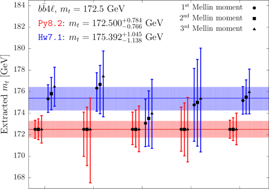
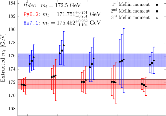
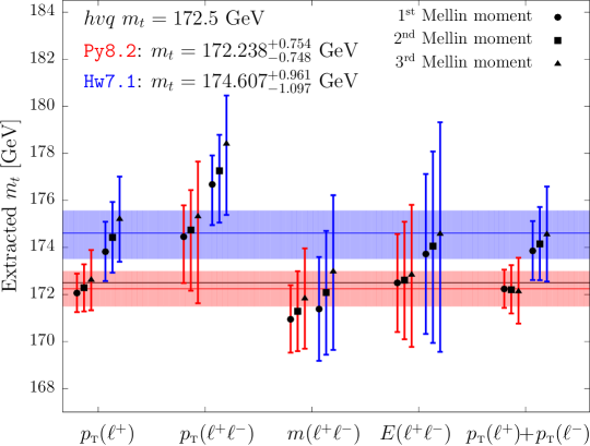
Figure 14.1: Extracted mass for the three generators matched with Pythia8.2 (red) and Herwig7.1 (blue) using the first three Mellin moments of the five leptonic observables. The horizontal band represents the weighted average of the results, and the black horizontal line corresponds to $m_{t}=172.5$ GeV, which is the top mass value used in the $b\bar{b}4\ell$+Pythia8.2 reference sample.

As we did for $m_{Wb_{j}}^{\max}$ and $E_{b_{j}}^{\max}$, also in the present case we have computed the leptonic observables without including hadronization effects, i.e. at parton-shower only level, in order to determine whether the differences between Pythia8.2 and Herwig7.1 are due to the shower or to the hadronization. Our findings are summarized in Tab. 14.6. Most of the differences already arise at the shower level, this is not surprising since the hadronization and the underlying event does not alter the leptons momenta.

As for the previous observables, we have studied the effect of changing the matching scheme in decay, by switching between our two alternative matching schemes with Pythia8.2 and Herwig7.1, and by considering the settings of eq. (E.27) in Herwig7.1. In both cases we find results that are consistent within statistical errors.

We also evaluate the impact of the PowhegHooks veto for radiation in production, the results are presented in Tab. 14.7. Like for the $m_{Wb_{j}}^{\max}$ case, the differences between the two alternatives are very small, in particular, given the present statistical error, it is not negligible only for the $p_{\perp}$ of the lepton pair. Furthermore, the discrepancies are roughly the same for each NLO generator. Thus, our previous conclusions will not be modified by the use of PowhegHooks to deal with radiation in the production process.

		Py8.2 ${}-$ Hw7.1 [MeV]
observable​​	gen	full	PS only
	$b\bar{b}4\ell$	$+549\pm 70$	$+563\pm 71$
$\langle p_{\perp}(\ell^{+})\rangle$	$t\bar{t}dec$	$+605\pm 57$	$+609\pm 48$
	$hvq$	$+340\pm 45$	$+376\pm 46$
	$b\bar{b}4\ell$	$+1094\pm 83$	$+1092\pm 84$
$\langle p_{\perp}(\ell^{+}\ell^{-})\rangle$	$t\bar{t}dec$	$+1027\pm 65$	$+1020\pm 59$
	$hvq$	$+636\pm 54$	$+662\pm 55$
	$b\bar{b}4\ell$	$+188\pm 140$	$+286\pm 142$
$\langle m(\ell^{+}\ell^{-})\rangle$	$t\bar{t}dec$	$+736\pm 97$	$+814\pm 98$
	$hvq$	$+144\pm 90$	$+182\pm 91$
	$b\bar{b}4\ell$	$+1263\pm 229$	$+1342\pm 232$
$\langle E(\ell^{+}\ell^{-})\rangle$	$t\bar{t}dec$	$+1690\pm 160$	$+1712\pm 159$
	$hvq$	$+684\pm 148$	$+719\pm 150$
	$b\bar{b}4\ell$	$+1041\pm 134$	$+1091\pm 136$
$\langle p_{\perp}(\ell^{+})+p_{\perp}(\ell^{-})\rangle$	$t\bar{t}dec$	$+1143\pm 99$	$+1173\pm 92$
	$hvq$	$+629\pm 86$	$+690\pm 88$

Table 14.6: Differences between the Pythia8.2 and Herwig7.1 results for the leptonic observables, at full hadron level and at parton-level only.

— PowhegHooks ${}{-}$ no PowhegHooks [MeV]
— observable	$b\bar{b}4\ell$	$t\bar{t}dec$	$hvq$
$\phantom{\Big{|}}\langle p_{\perp}(\ell^{+})\rangle$	$57\pm 70$	$74\pm 47$	$50\pm 46$
$\phantom{\Big{|}}\langle p_{\perp}(\ell^{+}\ell^{-})\rangle$	$166\pm 84$	$173\pm 56$	$150\pm 54$
$\phantom{\Big{|}}\langle m(\ell^{+}\ell^{-})\rangle$	$25\pm 140$	$16\pm 91$	$-18\pm 90$
$\phantom{\Big{|}}\langle E(\ell^{+}\ell^{-})\rangle$	$145\pm 230$	$143\pm 152$	$123\pm 149$
$\phantom{\Big{|}}\langle p_{\perp}(\ell^{+})+p_{\perp}(\ell^{-})\rangle$	$123\pm 135$	$144\pm 89$	$107\pm 87$

Table 14.7: Differences between the leptonic observables obtained using the POWHEG:veto = 1 and the POWHEG:veto = 0 settings for the three generators interfaced with Pythia8.2.

Chapter 15 Summary and outlook

In this second part of the thesis we have compared generators of increasing accuracy for the production and decay of $t\bar{t}$ pairs considering observables suitable for the measurement of the top mass. The generators that we have considered are:

• The $hvq$ generator [81], that implements NLO corrections in production for on-shell top quarks, and includes finite-width effects and spin correlations only in an approximate way, by smearing the on-shell kinematics with Breit-Wigner forms of appropriate width, and by generating the angular distribution of the decay products according to the associated tree-level matrix elements [89].

• The $t\bar{t}dec$ generator [90], that implements NLO corrections in production and decay in the narrow-width approximation. Spin correlations are included at NLO accuracy. Finite width effects are implemented by reweighting the NLO results using the tree-level matrix elements for the associated Born-level process, including however all finite width non-resonant and interference effects at the Born level for the given final state.

• The $b\bar{b}4\ell$ generator [91], that uses the full matrix elements for the production of the given final state, including all non-resonant diagrams and interference effects. This includes interference of QCD radiation in production and decay.

The main focus has been the study of the mass distribution of a particle-level reconstructed top, consisting of a lepton-neutrino pair and a $b$-quark jet with the appropriate flavour. The peak position of the mass of this system is our observable, that is loosely related to the top mass. We considered its distributions both at the particle level, and by assuming that experimental inaccuracies can be summarized by a simple smearing with a resolution function, a Gaussian with a width of 15 GeV, which is the typical resolution achieved on the top mass by the LHC collaborations. This observable is an oversimplified version of the mass observables that are used in direct top-mass measurements, that are the methods that lead to the most precise mass determinations.

We have found a very consistent picture in the comparison of our three generators when they are interfaced to Pythia8.2, and thus we begin by summarizing our results for this case. We first recall what we expect from such comparison. When comparing the $hvq$ and the $t\bar{t}dec$ generators, we should remember that the latter has certainly better accuracy in the description of spin correlations, since it implements them correctly both at the leading and at the NLO level. However, we do not expect spin correlations to play an important role in the reconstructed top mass. As a further point, the $t\bar{t}dec$ generator implements NLO corrections in decay. In the $hvq$ generator, the decay is handled by the shower, where, by default, Pythia8.2 includes matrix-element corrections (MEC). These differ formally from a full NLO correction only by a normalization factor, that amounts to the NLO correction to the top width. Thus, as long as the MEC are switched on, we do not expect large differences between $hvq$ and $t\bar{t}dec$. As far as the comparison between $t\bar{t}dec$ and $b\bar{b}4\ell$, we expect the difference to be given by NLO off-shell effects, and by interference of radiation in production and decay, since these effects are not implemented in $t\bar{t}dec$. This comparison is particularly interesting, since the interference between production and decay can be considered as a “perturbative precursor” of colour reconnection effects.

The results of these comparisons can be summarized as follows:

• The $t\bar{t}dec$ and the $b\bar{b}4\ell$ generators yield very similar results for most of the observables that we have considered, implying that NLO off-shell effects and interference between production and decay are modest.

• As far as $m_{Wb_{j}}^{\max}$ (the peak of the reconstructed mass distribution) is concerned, the $t\bar{t}dec$ and the $hvq$ generators yield very similar results, confirming the fact that the MEC implementation in Pythia8.2 has an effect very similar to the POWHEG implementation of NLO corrections in decay in the $t\bar{t}dec$. We have also observed that, if we switch off the MEC, the agreement between the two generators is spoiled. More quantitatively, we find that the spread in the peak of the reconstructed mass at the particle level among the three NLO+PS generators is never above 30 MeV. On the other hand, if resolution effects are accounted for with our smearing procedure, we find that the $hvq$ result is 147 MeV smaller, and the $t\bar{t}dec$ result 140 MeV larger than the $b\bar{b}4\ell$ one. These values are safely below currently quoted errors for the top-mass measurements with direct methods.

  If we switch off the MEC in Pythia8.2, we find that the peak position at the particle level in the $hvq$ case is displaced by 61 MeV, while, if smearing effects are included, the shift is of $916$ MeV, a rather large value, that can however be disregarded as being due to the poor accuracy of the collinear approximation in $b$ radiation when MEC corrections are off.

• The jet-energy peak seems to be more sensitive to the modelling of radiation from the $b$ quark. In fact, while the $t\bar{t}dec$ and the $b\bar{b}4\ell$ results are quite consistent with each other, with the peak positions differing by less than 200 MeV, the $hvq$ result differs from them by more than 500 MeV. This would correspond to a difference in the extracted mass of the top quark roughly equal to twice that amount. On the other hand, if the MEC in $hvq$ are switched off, the shift in the $b$-jet energy peak is more than 1.9 GeV. This leads us to conclude that the impact of modelling of $b$ radiation on the $b$-jet peak is much stronger than in the reconstructed top mass peak. We stress, however, that the difference between $hvq$ (with MEC on) and the other two generators is safely below the errors quoted in current measurements [73].

• For the leptonic observables, we generally see a reasonable agreement between the different generators. The largest differences are found in the $hvq$ case, for the $p_{\perp}(\ell^{+}\ell^{-})$ and $m(\ell^{+}\ell^{-})$, larger than 500 MeV with respect to the other two. In Ref. [68] it was noticed that these observables had larger errors due to a stronger sensitivity to radiative corrections, and to spin-correlation effects, that are modelled incorrectly by $hvq$.

Several sources of possible uncertainties have been explored in order to check the reliability of these conclusions. First of all, two different matching procedures for interfacing the $t\bar{t}dec$ and $b\bar{b}4\ell$ generators to Pythia8.2 have been implemented. For example, for the reconstructed mass peak, we have checked that switching between them leads to differences below 20 MeV for both generators. The effect of scales, $\alpha_{s}$ and PDF uncertainties have also been examined, and were found to yield very modest variations in the reconstructed mass peak. It was found, in particular, that scale variations lead to a negligible peak displacement (below 7 MeV) in the $t\bar{t}dec$ and $hvq$ case, while the effect is of ${}^{+86}_{-53}$ MeV for $b\bar{b}4\ell$. The lack of scale dependence in the $hvq$ and $t\bar{t}dec$ is easily understood as being due to the fact that the peak shape is obtained by smearing an on-shell distribution with a Breit-Wigner form, that does not depend upon any scale, and it suggests that, in order to get realistic scale-variation errors, the most accurate $b\bar{b}4\ell$ generator should be used. We have also computed results at the shower level, excluding the effects of hadronization and multi-parton interactions, in order to see if the consistent picture found at the hadron level is also supported by the parton-level results, and we have found that this is indeed the case.

We have thus seen that the overall picture of the comparison of our three NLO+PS generators within the framework of the Pythia8.2 shower is quite simple and consistent. For the most precise observable, i.e. the peak of the reconstructed mass distribution, it leads to the conclusions that the use of the most accurate generator may lead to a shift in the measured mass of at most 150 MeV, which is well below the present uncertainties quoted by the experimental collaborations.

Our study with Herwig7.1 instead reveals several problems. We can summarize our findings as follows:

• The results obtained with Herwig7.1 differ substantially from those obtained with Pythia8.2. In particular, the peak of the reconstructed mass distribution at the particle level is shifted by -66 and -39 MeV in the $b\bar{b}4\ell$ and $t\bar{t}dec$ cases, and by +235 MeV in the $hvq$ case. When the experimental resolution is accounted for, using our smearing procedure, the shift raises to -1091 and -1179 MeV in the $b\bar{b}4\ell$ and $t\bar{t}dec$ cases, and to -251 MeV in the $hvq$ case.

• The results obtained within the Herwig7.1 framework display large differences between the $hvq$ generator with respect to $b\bar{b}4\ell$ and $t\bar{t}dec$ ones. In particular, while the $t\bar{t}dec$ result exceeds the $b\bar{b}4\ell$ one only by about 50 MeV in both the particle level and smeared cases, $hvq$ exceeds $b\bar{b}4\ell$ by 311 MeV at particle level, and by 693 MeV after smearing.

These results are quite alarming. The shifts reach values that are considerably larger than current experimental uncertainties.

In the $hvq$ case, which is the NLO+PS generator currently used for top-mass studies by the experimental collaborations, the difference in the mass-peak position between Herwig7.1 and Pythia8.2, for the smeared distribution, is -251 MeV, uncomfortably large but still below current errors. One would then be tempted to conclude that the large shifts may be linked to some problems concerning the new generators. However, we also notice that the same difference is +235 MeV when no smearing is applied, so it is about as large in magnitude but with the opposite sign. This indicates that the shape of the reconstructed mass distribution is considerably different in the two shower models. Lastly, if we use the internal POWHEG implementation of top decay (rather than the MEC) in Herwig7.1, the difference with respect to Pythia8.2 raises to 607 MeV. Thus, we conclude that in the $hvq$ case the smaller difference between Herwig7.1 and Pythia8.2 is accidental, and is subject to considerable variations depending upon the settings.

Also in this case we checked whether the MEC yield an improved agreement between the $hvq$ and the other two generators, as was observed for Pythia8.2. We find that, by switching off MEC, the $hvq$+Herwig7.1 result decreases by 307 MeV at particle level, and by 1371 MeV in the smeared case. These effects are qualitatively similar to what was observed in Pythia8.2. However, in the present case, when MEC are switched off, the $hvq$ result exceeds the $b\bar{b}4\ell$ one by a negligible amount at the particle level, and is lower than the $b\bar{b}4\ell$ one by 678 MeV in the smeared case.

The discrepancy between $hvq$ and the other two generators is mitigated if, instead of the MEC procedure, the internal POWHEG option of Herwig7.1 for top decay is used. In this case, the discrepancy between $hvq$ and $b\bar{b}4\ell$ is reduced to 244 MeV with no smearing, and to 337 MeV with smearing. We thus see that the consistency of the three NLO+PS generators interfaced to Herwig7.1 is not optimal as in Pythia8.2. It is however acceptable if the internal POWHEG feature is used rather than MEC in Herwig7.1.

We have performed several studies to determine the origin of the difference between Pythia8.2 and Herwig7.1, and to check whether it could be attributed to some problem in our matching procedure. They can be summarized as follows:

• We have shown that the difference is mostly due to the shower model, since it is already largely present at the parton level.

• We have considered the $R$ dependence of the Herwig7.1 result. It differs from the one in Pythia8.2, leading to the hope that both generators may not represent the same set of data well, and tuning them may reduce their differences. However, we have also noticed that the difference in slope is much smaller than the difference in size.

• We have already mentioned that we have also compared results by making use of the internal POWHEG implementation of top decay in Herwig7.1, rather than using MEC. We have found non-negligible differences in this case.

• We have implemented alternative veto procedure in the matching of Herwig7.1 with the NLO+PS generators. We found differences of the order of 200 MeV, not large enough to cover the discrepancy with Pythia8.2.

• When interfacing POWHEG generators to angular-ordered showers, in order to maintain the double-logarithmic accuracy of the shower, one should introduce the so called “truncated showers” [98]. One could then worry that the lack of truncated showers is at the origin of the discrepancies that we found. Fortunately, Herwig7.1 offers some optional settings that are equivalent to the introduction of truncated showers. We found that these options lead to a shift of only 200 MeV in the peak position.

In summary, we found no indication that the discrepancy with Pythia8.2 is due to the specific matching procedure and general settings that we have used in Herwig7.1.

When comparing Herwig7.1 and Pythia8.2 in the computation of the $b$-jet energy peak, we have found even larger differences: when using $b\bar{b}4\ell$ and $t\bar{t}dec$, the shifts are of the order of 2 GeV, while for $hvq$ the shift is around 1 GeV. They correspond to differences in the extracted mass of around 4 GeV in the first two cases, and 2 GeV in the last one. This is not surprising, in view of the stronger sensitivity of the $b$-jet peak to the shower model.

Finally, when considering leptonic observables, we find again large differences between Herwig7.1 and Pythia8.2. Most differences already arise at the shower level. Notice that this is in contrast with the naive view that leptonic observables should be less dependent upon QCD radiation effects and jet modelling. The comparison between Herwig7.1 and Pythia8.2 for leptonic observables can by appreciated by looking at Fig. 14.1, representing the value of the extracted top mass from a sample generated with $b\bar{b}4\ell$ interfaced to Pythia8.2.

Chapter 16 Conclusions

We focus our conclusions on the results obtained for the reconstructed mass peak, since the issues that we have found there apply to the direct top mass measurements, that are the most precise. The experimental collaborations extensively use the $hvq$ generator for this kind of analyses, and since new generators of higher accuracy, the $t\bar{t}dec$ and the $b\bar{b}4\ell$ ones, have become available, we have addressed the question of whether the physics effects not included in $hvq$ may lead to inaccuracies in the top-mass determination. The answer to this question is quite simple and clear when our generators are interfaced to Pythia8.2. The differences that we find are large enough to justify the use of the most accurate generators, but not large enough to drastically overturn the conclusions of current measurements. Notice that, since the $hvq$ generator does not include NLO corrections in decays, we might have expected a very different modelling of the $b$-jet in $hvq$ with respect to the other two generators, leading to important shifts in the extracted top mass value. It turns out, however, that the Pythia8.2 handling of top decay in $hvq$, improved with the matrix-element corrections, does in practice achieve NLO accuracy up to an irrelevant normalization factor.

This nicely consistent picture does not hold anymore if we use Herwig7.1 as shower generator. In particular, it seems that the MEC implemented in Herwig7.1 do not have the same effect as the handling of radiation in decay of our modern NLO+PS generators, leading to values of the extracted top mass that can differ up to about 700 MeV. Furthermore, interfacing our most accurate NLO+PS generator (the $b\bar{b}4\ell$ one) to Herwig7.1 leads to an extracted top mass of up to 1.2 GeV smaller with respect to the corresponding result with Pythia8.2.

At this point we have two options:

• Dismiss the Herwig7.1 results, on the ground that its MEC handling of top decay does not match our modern generators.

• Consider the Herwig7.1 result as a variation to be included as theoretical error.

We believe that the first option is not soundly motivated. In fact, the implementation of MEC in Pythia8.2 is also technically very close to what POWHEG does. The hardest radiation is essentially generated in the same way, and in both cases the subsequent radiation is generated with a lower transverse momentum. Thus the good agreement between the two is not surprising. The case of Herwig7.1 is completely different, since in angular-ordered showers the hardest radiation is not necessarily the first [54]. It is thus quite possible that the differences we found when Herwig7.1 handles the decay with MEC, with respect to the case when POWHEG does, are due to the fact that the two procedures, although formally equivalent (i.e. both leading to NLO accuracy) are technically different. In this last case, their difference should be attributed to uncontrolled higher-order effects, and should thus be considered as a theoretical uncertainty.

A further question that this analysis raises is whether we should consider the variation between the Pythia8.2 and the Herwig7.1 programs as an error that should be added to current top-mass measurements. By doing so, current errors, that are of the order of 500-600 MeV, would become larger than 1 GeV. We believe that our crude modelling of the measurement process does not allow us to draw this conclusion. The analysis procedures used in direct measurements are much more complex, and involve adequate tuning of the MC parameters and jet-energy calibration using hadronic $W$ decays in the same top events. It is not unlikely that these procedures could lead to an increased consistency between the Pythia8.2 and Herwig7.1 results. However, in view of what we have found in our study, it is difficult to trust the theoretical errors currently given in the top quark mass determination if alternative NLO+PS and shower generators combinations are not considered.

Part III Appendix

Appendix A Radiative corrections to quark lines

In this appendix we describe how to treat radiative corrections to external quark lines and how to compute the mass counterterm.

We denote by $\Sigma(\not{p},m_{b})$ the set of all the one-particle-irreducible corrections to an heavy quark line whose bare mass is $m_{b}$. If we include all the possible self-energy $\Sigma(\not{p},m_{b})$ insertions into a free propagator we obtain the expression for the dressed propagator

$$G(\not{p},m_{b}) = \frac{i}{\not{p}-m_{b}}+\frac{i}{\not{p}-m_{b}}\Sigma(\not{p},m_{b})\frac{i}{\not{p}-m_{b}}+\dots$$ (A.1)

$$= \frac{i}{\not{p}-m_{b}}\sum_{i=0}^{\infty}\left[i\Sigma(\not{p})\frac{1}{\not{p}-m_{b}}\right]^{n}\,=\,\frac{i}{\not{p}-m_{b}-i\Sigma(\not{p},m_{b})}\,,$$

where we have used the fact that $\Sigma(\not{p},m_{b})$ commutes with $\not{p}$. The location of the pole of the full propagator, i.e. the pole mass $m$, is equal to eigenvalue of the operator $\not{p}$ that satisfies

$$\left[\not{p}-m_{b}-i\Sigma(\not{p},m_{b})\right]_{\not{p}=m}\rightarrow m=m_{b}+i\Sigma(m,m_{b}).$$ (A.2)

We can introduce a mass counterterm $m^{c}$

$$m^{c}\!\equiv-i\,\Sigma\!\left(m,m_{b}\right),$$ (A.3)

so that we can replace in our Lagrangian

$$m_{b}\to m+m^{c}.$$ (A.4)

The Feynman rule for the mass counterterm is thus defined as the insertion, in the fermion propagator, of the vertex $-im^{c}$.

At order $\mathcal{O}(\alpha_{\mathchoice{\displaystyle}{\scriptstyle}{\scriptscriptstyle}{\scriptscriptstyle}\rm S})$

$$\Sigma\!\left(m,m_{b}\right)\approx\Sigma\!\left(m_{b},m_{b}\right)\approx\Sigma\!\left(m,m\right),$$ (A.5)

so that

$$m^{c}=-i\,\Sigma\!\left(m,m\right)+\mathcal{O}(\alpha_{\mathchoice{\displaystyle}{\scriptstyle}{\scriptscriptstyle}{\scriptscriptstyle}\rm S}^{2}).$$ (A.6)

The dressed propagator expressed in terms of the pole mass is thus given by

$$G^{r}(\not{p},m)=\frac{i}{\not{p}-m-i\Sigma(\not{p},m_{b})-m^{c}},$$ (A.7)

that has a pole for $\not{p}=m$. If we consider eigenvalues of $\not{p}$ slightly different from $m$, the propagator becomes

$$G^{r}(\not{p},m) \approx \frac{i}{\not{p}-m-i\Sigma(m,m_{b})-z\left(\not{p}-m\right)-m^{c}}$$ (A.8)

$$= \frac{i}{\not{p}-m}(1-z)^{-1}\equiv\frac{i}{\not{p}-m}Z,$$

where we have defined

$$z\equiv i\frac{\partial\Sigma(\not{p},m_{b})}{\partial\not{p}}\Big{|}_{\not{p}=m}.$$ (A.9)

If we introduce the rescaled field $\phi_{r}$

$$\phi=Z^{1/2}\phi_{r},$$ (A.10)

we have the effect of the fermion self-energy correction to an external line is equivalent to multiply the leading order amplitude for a factor $Z^{1/2}$. At order $\mathcal{O}(\alpha_{\mathchoice{\displaystyle}{\scriptstyle}{\scriptscriptstyle}{\scriptscriptstyle}\rm S})$

$$Z=(1-z)^{-1}\approx 1+z,\qquad\sqrt{Z}\approx 1+\frac{1}{2}z,$$ (A.11)

where, neglecting orders $\mathcal{O}(\alpha_{\mathchoice{\displaystyle}{\scriptstyle}{\scriptscriptstyle}{\scriptscriptstyle}\rm S}^{2})$, we have

$$z\approx i\frac{\partial\Sigma(\not{p},m)}{\partial\not{p}}\Big{|}_{\not{p}=m}.$$ (A.12)

Thus, the contribution to the virtual amplitude containing radiative corrections to an external quark line is given by

$$\frac{1}{2}z\mathcal{M}_{b},$$ (A.13)

being $\mathcal{M}_{b}$ the LO amplitude.

An alternative to the pole mass scheme is given by the $\overline{\rm MS}$ scheme. The mass counterterm is defined in order to absorb only the divergent part of $\Sigma$ (performing the replacement $\mu^{2}\to\mu^{2}\frac{e^{{\gamma_{\mathchoice{\displaystyle}{\scriptstyle}{\scriptscriptstyle}{\scriptscriptstyle}E}}}}{4\pi}$)

$$\overline{m}^{c}(\mu) \equiv -i\,\Sigma^{\rm(d)}\!\left(\overline{m}(\mu),m_{b}\right)=-i\,\Sigma^{\rm(d)}\!\left(m,m\right)+\mathcal{O}(\alpha_{\mathchoice{\displaystyle}{\scriptstyle}{\scriptscriptstyle}{\scriptscriptstyle}\rm S}^{2})\,,$$ (A.14)

where $\overline{m}(\mu)$ is the $\overline{\rm MS}$ mass evaluated at the scale $\mu$ and (d) denotes the divergent part. We have

$$m_{b}=m+m^{c}=\overline{m}(\mu)+\overline{m}^{c}(\mu),$$ (A.15)

$$m-\overline{m}(\mu)=-\left[m^{c}-\overline{m}^{c}(\mu)\right]=i\,\Sigma^{\rm(f)}\!\left(m,m\right)+\mathcal{O}(\alpha_{\mathchoice{\displaystyle}{\scriptstyle}{\scriptscriptstyle}{\scriptscriptstyle}\rm S}^{2}),$$ (A.16)

where (f) denotes the finite part.

A.1 One-loop radiative corrections to heavy quark lines

In the following we describe how to compute the one-loop on-shell top-quark self energy at order $\alpha_{\mathchoice{\displaystyle}{\scriptstyle}{\scriptscriptstyle}{\scriptscriptstyle}\rm S}$. We give a finite mass $\lambda$ to the gluon, since this result is necessary for the computation of the self energy at all orders in $\alpha_{\mathchoice{\displaystyle}{\scriptstyle}{\scriptscriptstyle}{\scriptscriptstyle}\rm S}(\alpha_{\mathchoice{\displaystyle}{\scriptstyle}{\scriptscriptstyle}{\scriptscriptstyle}\rm S}n_{f})^{n}$, as discussed in Sec. 3.2. Since we adopt the $\overline{\rm MS}$ scheme, in our computation we perform the replacement

$$\mu^{2}\to\mu^{2}\frac{e^{\epsilon{\gamma_{\mathchoice{\displaystyle}{\scriptstyle}{\scriptscriptstyle}{\scriptscriptstyle}E}}}}{4\pi}$$ (A.17)

so that, as we have seen in Sec. 3.1, the $\overline{\rm MS}$ counterterms have a very simple expression since they need to absorb only the UV divergent part of the radiative corrections.

At order $\alpha_{\mathchoice{\displaystyle}{\scriptstyle}{\scriptscriptstyle}{\scriptscriptstyle}\rm S}{}$, the top-quark self-energy expression with a gluon of mass $\lambda$ in $d=4-2\epsilon$ dimensions is given by

$$\!\!\!\!\!\!\!\Sigma^{(1)}_{\lambda}(\not{p},m)= \,-g^{2}C_{\mathchoice{\displaystyle}{\scriptstyle}{\scriptscriptstyle}{\scriptscriptstyle}\rm F}\left(\frac{\mu^{2}}{4\pi}e^{{\gamma_{\mathchoice{\displaystyle}{\scriptstyle}{\scriptscriptstyle}{\scriptscriptstyle}E}}}\right)^{\epsilon}\int\frac{\mathrm{d}^{d}k}{(2\pi)^{d}}\frac{\gamma^{\alpha}(\not{p}+\not{k}+m)\gamma_{\alpha}}{\left[k^{2}-\lambda^{2}\right]\left[(k+p)^{2}-m^{2}\right]}$$

$$= \,-g^{2}C_{\mathchoice{\displaystyle}{\scriptstyle}{\scriptscriptstyle}{\scriptscriptstyle}\rm F}\left(\frac{\mu^{2}}{4\pi}e^{{\gamma_{\mathchoice{\displaystyle}{\scriptstyle}{\scriptscriptstyle}{\scriptscriptstyle}E}}}\right)^{\epsilon}\int\frac{\mathrm{d}^{d}k}{(2\pi)^{d}}\frac{(2-d)\not{p}+d\,m+(2-d)\not{k}}{\left[k^{2}-\lambda^{2}\right]\left[(k+p)^{2}-m^{2}\right]}$$ (A.18)

$$= \,-g^{2}C_{\mathchoice{\displaystyle}{\scriptstyle}{\scriptscriptstyle}{\scriptscriptstyle}\rm F}\left[(2-d)\not{p}\frac{(m^{2}-\lambda^{2}-p^{2})B(p^{2},\lambda^{2},m^{2})+A(\lambda^{2})-A(m^{2})}{2p^{2}}\right.$$

$$\,\phantom{-g^{2}C_{\mathchoice{\displaystyle}{\scriptstyle}{\scriptscriptstyle}{\scriptscriptstyle}\rm F}\bigg{[}}+\left((2-d)\not{p}+d\,m\right)B(p^{2},\lambda^{2},m^{2})\bigg{]}\,,$$ (A.19)

where the suffix $\lambda$ signals the presence of a finite gluon-mass $\lambda$ and $A$ and $B$ are the one-point and two-point Feynmam scalar integrals

$$A(m^{2}) = \left(\frac{\mu^{2}}{4\pi}e^{{\gamma_{\mathchoice{\displaystyle}{\scriptstyle}{\scriptscriptstyle}{\scriptscriptstyle}E}}}\right)^{\epsilon}\int\frac{\mathrm{d}^{d}k}{(2\pi)^{d}}\frac{1}{k^{2}-m^{2}}\,,$$ (A.20)

$$B(p^{2},\lambda^{2},m^{2}) = \left(\frac{\mu^{2}}{4\pi}e^{{\gamma_{\mathchoice{\displaystyle}{\scriptstyle}{\scriptscriptstyle}{\scriptscriptstyle}E}}}\right)^{\epsilon}\int\frac{\mathrm{d}^{d}k}{(2\pi)^{d}}\frac{1}{\left[k^{2}-\lambda^{2}\right]\left[(k+p)^{2}-m^{2}\right]}\,.$$ (A.21)

A.2 Mass counterterm

From eq. (A.6), we see that the pole mass counterterm can be obtained from the self energy evaluated for the eigenvalue of the operator $\not{p}$ equal to $m$. We thus compute $\Sigma_{\lambda}^{(1)}(m,m)$. As it is shown in Sec. 3.2, we also need the exact $d$-dimensional expression for the $\lambda=0$ and $\lambda\gg m$ cases, while for a generic $\lambda$ value it is sufficient the $\mathcal{O}(\epsilon^{0})$ expressions.

A.2.1 Non-vanishing gluon mass

We now calculate $\Sigma^{(1)}_{\lambda}(m,m)$ for a generic value of $\lambda>0$. Eq. (A.19) becomes

$$\Sigma^{(1)}_{\lambda}(m,m) = -g^{2}\,C_{\mathchoice{\displaystyle}{\scriptstyle}{\scriptscriptstyle}{\scriptscriptstyle}\rm F}\,m\,\left[(2-d)\frac{-\lambda^{2}\,B(m^{2},\lambda^{2},m^{2})+A(\lambda^{2})-A(m^{2})}{2m^{2}}\right.$$ (A.22)

$$\phantom{-g^{2}\,C_{\mathchoice{\displaystyle}{\scriptstyle}{\scriptscriptstyle}{\scriptscriptstyle}\rm F}\,m\,\Big{[}}\left.+d\,B(m^{2},\lambda^{2},m^{2})\right]\qquad$$

and the scalar integrals assume the values

$$A(m^{2}) = \frac{i}{(4\pi)^{2}}\,m^{2}\,\left[\frac{1}{\epsilon}+\log\left(\frac{\mu^{2}}{m^{2}}\right)+1\right]+\mathcal{O}(\epsilon),$$ (A.23)

$$B(m^{2},\lambda^{2},m^{2}) = \frac{i}{(4\pi)^{2}}\left[\frac{1}{\epsilon}+2+\log\left(\frac{\mu^{2}}{m^{2}}\right)+H\left(\frac{\lambda^{2}}{m^{2}}\right)\right]+\mathcal{O}(\epsilon),$$ (A.24)

with

$$H(x)=\left\{\begin{array}[]{ll}\displaystyle{-\frac{x}{2}\log{x}-\sqrt{x(4-x)}\,\arctan\sqrt{\frac{4-x}{x}}}&x\leq 4\,,\\[5.69054pt] \displaystyle{-\frac{x}{2}\,\log{x}+\frac{1}{2}\sqrt{x(x-4)}\log\frac{\sqrt{x}+\sqrt{x-4}}{\sqrt{x}-\sqrt{x-4}}}&x>4\,.\end{array}\right.$$ (A.25)

We can check that for small $x$

$$H(x)=-\pi\sqrt{x}+\mathcal{O}(x)\,,$$ (A.26)

while for large $x$

$$H(x)=-1-\log(x)+\frac{1}{x}\left(\frac{1}{2}-\log(x)\right)+\mathcal{O}\left(\frac{1}{x^{2}}\right).$$ (A.27)

Substituting the values of $A$ and $B$ in eq. (A.22), we get

$$\Sigma^{(1)}_{\lambda}(m,m) = -i\,\frac{\alpha_{\mathchoice{\displaystyle}{\scriptstyle}{\scriptscriptstyle}{\scriptscriptstyle}\rm S}}{4\pi}C_{\mathchoice{\displaystyle}{\scriptstyle}{\scriptscriptstyle}{\scriptscriptstyle}\rm F}\,m\left[\frac{3}{\epsilon}+3\log\left(\frac{\mu^{2}}{m^{2}}\right)+4+\frac{\lambda^{2}}{m^{2}}\left(1+\log\left(\frac{\lambda^{2}}{m^{2}}\right)\right)\right.\qquad$$ (A.28)

$$\phantom{-i\,\frac{\alpha_{\mathchoice{\displaystyle}{\scriptstyle}{\scriptscriptstyle}{\scriptscriptstyle}\rm S}}{4\pi}C_{\mathchoice{\displaystyle}{\scriptstyle}{\scriptscriptstyle}{\scriptscriptstyle}\rm F}\,m\Big{[}}\left.+\left(2+\frac{\lambda^{2}}{m^{2}}\right)H\left(\frac{\lambda^{2}}{m^{2}}\right)\right]\,.\qquad$$

For small $\lambda$ we have

$$\Sigma^{(1)}_{\lambda}(m,m)=-i\frac{\alpha_{\mathchoice{\displaystyle}{\scriptstyle}{\scriptscriptstyle}{\scriptscriptstyle}\rm S}}{4\pi}C_{\mathchoice{\displaystyle}{\scriptstyle}{\scriptscriptstyle}{\scriptscriptstyle}\rm F}\,m\left[\frac{3}{\epsilon}+3\log\left(\frac{\mu^{2}}{m^{2}}\right)+4\right]+\alpha_{\mathchoice{\displaystyle}{\scriptstyle}{\scriptscriptstyle}{\scriptscriptstyle}\rm S}\frac{C_{\mathchoice{\displaystyle}{\scriptstyle}{\scriptscriptstyle}{\scriptscriptstyle}\rm F}}{2}\lambda+\mathcal{O}(\lambda^{2})\,,\qquad$$ (A.29)

while for large $\lambda$

$$\Sigma^{(1)}_{\lambda}(m,m)=-i\frac{\alpha_{\mathchoice{\displaystyle}{\scriptstyle}{\scriptscriptstyle}{\scriptscriptstyle}\rm S}}{4\pi}C_{\mathchoice{\displaystyle}{\scriptstyle}{\scriptscriptstyle}{\scriptscriptstyle}\rm F}\,m\left[\frac{3}{\epsilon}+3\log\left(\frac{\mu^{2}}{\lambda^{2}}\right)+\frac{5}{2}\right]+\mathcal{O}\left(\frac{1}{\lambda^{2}}\right)\,.\qquad$$ (A.30)

We thus have that the mass counterterm in the pole scheme, computed keeping a fixed gluon mass $\lambda$, is given by

$$m^{c}_{\lambda} = -i\,\Sigma^{(1)}_{\lambda}(m,m)$$ (A.31)

$$= -\frac{\alpha_{\mathchoice{\displaystyle}{\scriptstyle}{\scriptscriptstyle}{\scriptscriptstyle}\rm S}}{4\pi}C_{\mathchoice{\displaystyle}{\scriptstyle}{\scriptscriptstyle}{\scriptscriptstyle}\rm F}\,m\left[\frac{3}{\epsilon}+3\log\left(\frac{\mu^{2}}{m^{2}}\right)+4+\frac{\lambda^{2}}{m^{2}}\left(1+\log\left(\frac{\lambda^{2}}{m^{2}}\right)\right)\right.$$

$$\phantom{-\frac{\alpha_{\mathchoice{\displaystyle}{\scriptstyle}{\scriptscriptstyle}{\scriptscriptstyle}\rm S}}{4\pi}C_{\mathchoice{\displaystyle}{\scriptstyle}{\scriptscriptstyle}{\scriptscriptstyle}\rm F}\,m\Big{[}}\left.+\left(2+\frac{\lambda^{2}}{m^{2}}\right)H\left(\frac{\lambda^{2}}{m^{2}}\right)\right]\,.$$

A.2.2 Massless gluon

We are now interested in the particular case $\lambda=0$. By setting $\lambda=0$ in eq. (A.22), we find

$$\Sigma^{(1)}_{0}(m,m) = -g^{2}\,C_{\mathchoice{\displaystyle}{\scriptstyle}{\scriptscriptstyle}{\scriptscriptstyle}\rm F}\,m\,\left[-(2-d)\frac{A(m^{2})}{2m^{2}}+d\,B(m^{2},\lambda^{2},m^{2})\right]\,.$$ (A.32)

In this case, it is possible to use the exact $d$ dimensional expressions for the scalar integrals

$$A(m^{2}) = \frac{i}{(4\pi)^{2}}\Gamma(1+\epsilon)\,{\rm e}^{\epsilon{\gamma_{\mathchoice{\displaystyle}{\scriptstyle}{\scriptscriptstyle}{\scriptscriptstyle}E}}}\left(\frac{\mu^{2}}{m^{2}}\right)^{\epsilon}\frac{m^{2}}{\epsilon\,(1-\epsilon)}\,,$$ (A.33)

$$B(m^{2},0,m^{2}) = \frac{i}{(4\pi)^{2}}\Gamma(1+\epsilon)\,{\rm e}^{\epsilon{\gamma_{\mathchoice{\displaystyle}{\scriptstyle}{\scriptscriptstyle}{\scriptscriptstyle}E}}}\left(\frac{\mu^{2}}{m^{2}}\right)^{\epsilon}\frac{m^{2}}{\epsilon\,(1-2\epsilon)}\,,$$ (A.34)

so that we find

$$\Sigma^{(1)}_{0}(m,m)=-i\frac{\alpha_{\mathchoice{\displaystyle}{\scriptstyle}{\scriptscriptstyle}{\scriptscriptstyle}\rm S}}{4\pi}C_{\mathchoice{\displaystyle}{\scriptstyle}{\scriptscriptstyle}{\scriptscriptstyle}\rm F}\,m\left(\frac{\mu^{2}}{m^{2}}\right)^{\epsilon}e^{\epsilon{\gamma_{\mathchoice{\displaystyle}{\scriptstyle}{\scriptscriptstyle}{\scriptscriptstyle}E}}}\frac{\Gamma(1+\epsilon)}{\epsilon}\frac{3-2\epsilon}{1-2\epsilon}\,.$$ (A.35)

By expanding around $\epsilon=0$ we get

$$\Sigma^{(1)}_{0}(m,m) \approx -i\,\frac{\alpha_{\mathchoice{\displaystyle}{\scriptstyle}{\scriptscriptstyle}{\scriptscriptstyle}\rm S}}{4\pi}C_{\mathchoice{\displaystyle}{\scriptstyle}{\scriptscriptstyle}{\scriptscriptstyle}\rm F}\,m\left[\frac{3}{\epsilon}+3\log\left(\frac{\mu^{2}}{m^{2}}\right)+4\right]\,.$$ (A.36)

By comparing this expression with eq. (A.29), we find that the small $\lambda$ result smoothly converges to the massless one. Since $\Sigma^{(1)}_{0}(m,m)$ corresponds to the standard result peformed with massless gluons, we have

$$\Sigma^{(1)}_{0}(m,m)\equiv\Sigma^{(1)}(m,m).$$ (A.37)

The pole mass counterterm is thus given by

$$m^{c}=-i\Sigma^{(1)}(m,m)=-\frac{\alpha_{\mathchoice{\displaystyle}{\scriptstyle}{\scriptscriptstyle}{\scriptscriptstyle}\rm S}}{4\pi}C_{\mathchoice{\displaystyle}{\scriptstyle}{\scriptscriptstyle}{\scriptscriptstyle}\rm F}\,m\left[\frac{3}{\epsilon}+3\log\left(\frac{\mu^{2}}{m^{2}}\right)+4\right]+\mathcal{O}(\alpha_{\mathchoice{\displaystyle}{\scriptstyle}{\scriptscriptstyle}{\scriptscriptstyle}\rm S}^{2}).$$ (A.38)

As shown in eq. (A.14), if we adopt the $\overline{\rm MS}$ scheme, the mass counterterm contains only the divergent part of $\Sigma^{(1)}$:

$$\overline{m}^{c}(\mu)=-\frac{\alpha_{\mathchoice{\displaystyle}{\scriptstyle}{\scriptscriptstyle}{\scriptscriptstyle}\rm S}}{4\pi}C_{\mathchoice{\displaystyle}{\scriptstyle}{\scriptscriptstyle}{\scriptscriptstyle}\rm F}\,\overline{m}(\mu)\,\frac{3}{\epsilon}+\mathcal{O}(\alpha_{\mathchoice{\displaystyle}{\scriptstyle}{\scriptscriptstyle}{\scriptscriptstyle}\rm S}^{2})\,,$$ (A.39)

and

$$m-\overline{m}(\mu)=-\left[m^{c}-\overline{m}^{c}(\mu)\right]=\frac{\alpha_{\mathchoice{\displaystyle}{\scriptstyle}{\scriptscriptstyle}{\scriptscriptstyle}\rm S}}{4\pi}C_{\mathchoice{\displaystyle}{\scriptstyle}{\scriptscriptstyle}{\scriptscriptstyle}\rm F}\,m\left[3\log\left(\frac{\mu^{2}}{m^{2}}\right)+4\right]+\mathcal{O}(\alpha_{\mathchoice{\displaystyle}{\scriptstyle}{\scriptscriptstyle}{\scriptscriptstyle}\rm S}^{2}).$$ (A.40)

A.2.3 Large gluon mass

In order to evaluate the exact $d$ dimensional expression of eq. (A.22) for large $\lambda$ we just need to compute $B(m^{2},\lambda^{2},m^{2})$ neglecting terms of order $\frac{m^{4}}{\lambda^{4}}$

$$B(m^{2},\lambda^{2},m^{2})= \,\left(\frac{\mu^{2}}{4\pi}\,{\rm e}^{{\gamma_{\mathchoice{\displaystyle}{\scriptstyle}{\scriptscriptstyle}{\scriptscriptstyle}E}}}\right)^{\epsilon}\int\frac{\mathrm{d}^{d}k}{(2\pi)^{d}}\frac{1}{(k+p)^{2}-m^{2}+i\eta}\frac{1}{k^{2}-\lambda^{2}+i\eta}$$

$$= \,\frac{i\,e^{\epsilon{\gamma_{\mathchoice{\displaystyle}{\scriptstyle}{\scriptscriptstyle}{\scriptscriptstyle}E}}}\Gamma(\epsilon)}{(4\pi)^{2}}\mu^{2\epsilon}\int_{0}^{1}[-z(1-z)\lambda^{2}+(1-z)\lambda^{2}+zm^{2}]^{-\epsilon}\mathrm{d}z$$

$$= \,\frac{i\,e^{\epsilon{\gamma_{\mathchoice{\displaystyle}{\scriptstyle}{\scriptscriptstyle}{\scriptscriptstyle}E}}}\Gamma(\epsilon)}{(4\pi)^{2}}\mu^{2\epsilon}\int_{0}^{1}[z^{2}m^{2}+(1-z)\lambda^{2}]^{-\epsilon}\mathrm{d}z$$

$$= \,\frac{i}{(4\pi)^{2}}\left(\frac{\mu^{2}}{m^{2}}\right)^{\epsilon}\,e^{\epsilon{\gamma_{\mathchoice{\displaystyle}{\scriptstyle}{\scriptscriptstyle}{\scriptscriptstyle}E}}}\,\Gamma(\epsilon)\int_{0}^{1}(\eta_{+}-z)^{-\epsilon}(\eta_{-}-z)^{-\epsilon}\mathrm{d}z,$$ (A.41)

where we have defined

$$\eta_{+}=\frac{1+\sqrt{1-4\xi}}{2\xi}\approx\frac{1}{\xi}-1,\hskip 20.00003pt\eta_{-}=\frac{1-\sqrt{1-4\xi}}{2\xi}\approx 1+\xi\hskip 10.00002pt,$$ (A.42)

with $\xi=m^{2}/\lambda^{2}$. For small $\xi$ the integral yields

$$\!\!\!\!\!\!\!\!\!\!\!\!\!\!\int_{0}^{1}(\eta_{+}-z)^{-\epsilon}(\eta_{-}-z)^{-\epsilon}\mathrm{d}z\approx \,\xi^{\epsilon}\int_{0}^{1}(1-\xi(1+z))^{-\epsilon}(1-z+\xi)^{-\epsilon}\mathrm{d}z$$

$$\approx \,\xi^{\epsilon}\int_{0}^{1}(1+\epsilon\,\xi(1+z))(1-z+\xi)^{-\epsilon}\mathrm{d}z$$

$$\approx \,\xi^{\epsilon}\left\{\frac{(1+\xi)^{1-\epsilon}-\xi^{1-\epsilon}}{1-\epsilon}+\epsilon\,\xi\int_{0}^{1}(1+z)(1-z)^{-\epsilon}\mathrm{d}z\right\}$$

$$= \,\xi^{\epsilon}\left\{\frac{1+(1-\epsilon)\xi-\xi^{1-\epsilon}}{1-\epsilon}+\epsilon\,\xi\frac{3-\epsilon}{(1-\epsilon)(2-\epsilon)}\right\}$$

$$= \,\xi^{\epsilon}\left\{\frac{1}{1-\epsilon}-\frac{\xi^{1-\epsilon}}{1-\epsilon}+\xi\left(1+\epsilon\frac{3-\epsilon}{(1-\epsilon)(2-\epsilon)}\right)\right\}$$

$$= \,\xi^{\epsilon}\left\{\frac{1}{1-\epsilon}-\frac{\xi^{1-\epsilon}}{1-\epsilon}+\xi\frac{2}{(1-\epsilon)(2-\epsilon)}\right\},$$ (A.43)

so

$$B(m^{2},\lambda^{2},m^{2}) = \frac{i}{(4\pi)^{2}}\left(\frac{\mu^{2}}{\lambda^{2}}\right)^{\epsilon}\,e^{\epsilon{\gamma_{\mathchoice{\displaystyle}{\scriptstyle}{\scriptscriptstyle}{\scriptscriptstyle}E}}}\,\frac{\Gamma(1+\epsilon)}{\epsilon}$$ (A.44)

$$\times\left[\frac{1}{1-\epsilon}-\left(\frac{m^{2}}{\lambda^{2}}\right)^{1-\epsilon}\frac{1}{1-\epsilon}+\frac{m^{2}}{\lambda^{2}}\frac{2}{(1-\epsilon)(2-\epsilon)}\right]\,.\qquad$$

By inserting eqs. (A.44) and (A.33) in eq. (A.22) and neglecting terms of the order $\lambda^{-2}$ we find

$$\Sigma_{\lambda_{\infty}}^{(1)}(m,m)=-i\frac{\alpha_{\mathchoice{\displaystyle}{\scriptstyle}{\scriptscriptstyle}{\scriptscriptstyle}\rm S}}{4\pi}C_{\mathchoice{\displaystyle}{\scriptstyle}{\scriptscriptstyle}{\scriptscriptstyle}\rm F}\,m\left(\frac{\mu^{2}}{\lambda^{2}}\right)^{\epsilon}\frac{\Gamma(1+\epsilon)\,e^{\epsilon{\gamma_{\mathchoice{\displaystyle}{\scriptstyle}{\scriptscriptstyle}{\scriptscriptstyle}E}}}}{\epsilon}\frac{2\,(3-2\epsilon)}{(1-\epsilon)(2-\epsilon)}\,,$$ (A.45)

where the subscript $\infty$ signals that $\Sigma$ has been computed for a large value of $\lambda$ and subleading powers $1/\lambda^{2}$ have been neglected. By expanding $\Sigma_{\lambda_{\infty}}^{(1)}(m,\lambda^{2})$ around $\epsilon=0$ we get

$$\Sigma_{\lambda_{\infty}}^{(1)}(m,m)\approx-i\,\frac{\alpha_{\mathchoice{\displaystyle}{\scriptstyle}{\scriptscriptstyle}{\scriptscriptstyle}\rm S}}{4\pi}C_{\mathchoice{\displaystyle}{\scriptstyle}{\scriptscriptstyle}{\scriptscriptstyle}\rm F}\,m\left[\frac{3}{\epsilon}+3\log\left(\frac{\mu^{2}}{\lambda^{2}}\right)+\frac{5}{3}\right]\,,$$ (A.46)

as we found in eq. (A.30).

A.3 External field normalization

From eqs. (A.11) and (A.12) we have that the external field normalization is given by

$$Z=1+z\,,\qquad{\rm with}\quad z=i\frac{\partial\Sigma(\not{p},m)}{\partial\not{p}}\Big{|}_{\not{p}=m}.$$ (A.47)

We perform this computation at $\mathcal{O}(\alpha_{\mathchoice{\displaystyle}{\scriptstyle}{\scriptscriptstyle}{\scriptscriptstyle}\rm S})$ keeping a finite gluon mass $\lambda$ and, separately, for $\lambda=0$. Conversely to the previous case, the small $\lambda$ limit is not guaranteed to approach smoothly the $\lambda=0$ result, since to compute $z$ we deal both with IR and UV singularities.

We rewrite eq. (A.19) as

$$\Sigma^{(1)}_{\lambda}(\not{p},m)=g^{2}C_{\mathchoice{\displaystyle}{\scriptstyle}{\scriptscriptstyle}{\scriptscriptstyle}\rm F}\left\{\alpha\,B(p^{2},\lambda^{2},m^{2})+\beta\left[A(\lambda^{2})-A(m^{2})\right]\right\}$$ (A.48)

with

$$\alpha=\frac{d-2}{2p^{2}}(m^{2}-\lambda^{2}-p^{2})\not{p}+(d-2)\not{p}-d\lambda,\qquad\qquad\beta=\frac{d-2}{2p^{2}}\not{p}\,.$$ (A.49)

Since $\not{p}\not{p}=p^{2}$, the derivative of with respect $\not{p}$ evaluated at $\not{p}=m$ can be rewritten as

$$\frac{\partial}{\partial\not{p}}\Bigg{|}_{\not{p}=m}=2m\frac{\partial}{\partial p^{2}}\Bigg{|}_{\not{p}=m}.$$ (A.50)

Using eq. (A.50) and

$$\alpha(\not{p}=m)=-m\left[2+(1-\epsilon)\frac{\lambda^{2}}{m^{2}}\right]\,,\quad\frac{\partial\alpha}{\partial\not{p}}\Bigg{|}_{\not{p}=m}=(1-\epsilon)\frac{\lambda^{2}}{m^{2}}\,,\quad\frac{\partial\beta}{\partial\not{p}}\Bigg{|}_{\not{p}=m}=\frac{\epsilon-1}{m^{2}}\,,\quad$$ (A.51)

eq. (A.48) becomes

$$\frac{\partial\Sigma^{(1)}_{\lambda}(\not{p},m)}{\partial\not{p}}\Bigg{|}_{\not{p}=m}= g^{2}\,C_{\mathchoice{\displaystyle}{\scriptstyle}{\scriptscriptstyle}{\scriptscriptstyle}\rm F}\left\{\frac{\lambda^{2}}{m^{2}}(1-\epsilon)B(m^{2},\lambda^{2},m^{2})+\frac{\epsilon-1}{m^{2}}\left[A(\lambda^{2})-A(m^{2})\right]\right.$$

$$\qquad\left.-m\left[2+(1-\epsilon)\frac{\lambda^{2}}{m^{2}}\right]\,2m\,\frac{\partial B(p^{2},\lambda^{2},m^{2})}{\partial p^{2}}\Big{|}_{p^{2}=m^{2}}\right\}.\qquad$$ (A.52)

The calculation of

$$\frac{\partial B(p^{2},\lambda^{2},m^{2})}{\partial m^{2}}\Big{|}_{p^{2}=m^{2}}$$

must be carried out by distinguishing the two cases $\lambda=0$ and $\lambda>0$.

A.3.1 Massless gluon

We need to compute the derivative of $B(p^{2},\lambda^{2},m^{2})$ for $p^{2}=m^{2}$ in order to evaluate the derivative of $\Sigma^{(1)}$. If $\lambda^{2}=0$, we have the well-known result

$$\frac{\partial B(p^{2},0,m^{2})}{\partial p^{2}}\Bigg{|}_{p^{2}=m^{2}} = \frac{i}{(4\pi)^{2}}\left(\frac{\mu^{2}}{m^{2}}\right)^{\epsilon}\frac{1}{m^{2}}\left[-\frac{1}{2\epsilon}-1\right]+\mathcal{O}(\epsilon)$$ (A.53)

$$= \frac{1}{(4\pi)^{2}}\frac{1}{m^{2}}\left[-\frac{1}{2\epsilon}-1-\frac{1}{2}\log\left(\frac{\mu^{2}}{m^{2}}\right)\right]+\mathcal{O}(\epsilon).\qquad$$

Substituting eqs. (A.53), (A.23) and the $\mathcal{O}(\epsilon^{0})$ expansion of eq. (A.34) in eq. (A.52) and setting $\lambda=0$ we find

$$\frac{\partial\Sigma^{(1)}(\not{p},m)}{\partial\not{p}}\Bigg{|}_{\not{p}=m}=i\frac{\alpha_{\mathchoice{\displaystyle}{\scriptstyle}{\scriptscriptstyle}{\scriptscriptstyle}\rm S}}{4\pi}\left[\frac{3}{\epsilon}+4+3\log\left(\frac{\mu^{2}}{m^{2}}\right)\right]\,.$$ (A.54)

So, from eq. (A.12), we get

$$z=i\frac{\partial\Sigma^{(1)}(\not{p},m)}{\partial\not{p}}\Bigg{|}_{\not{p}=m}=-\frac{\alpha_{\mathchoice{\displaystyle}{\scriptstyle}{\scriptscriptstyle}{\scriptscriptstyle}\rm S}}{4\pi}\left[\frac{3}{\epsilon}+4+3\log\left(\frac{\mu^{2}}{m^{2}}\right)\right]\,.$$ (A.55)

A.3.2 Massive gluon

We now compute the derivative of the bubble integral for $\lambda>0$.

$$\frac{\partial B(p^{2},\lambda^{2},m^{2})}{\partial p^{2}}\Bigg{|}_{p^{2}=m^{2}}=\frac{\partial}{\partial p^{2}}\left[\left(\mu^{2}\frac{e^{\epsilon{\gamma_{\mathchoice{\displaystyle}{\scriptstyle}{\scriptscriptstyle}{\scriptscriptstyle}E}}}}{4\pi}\right)^{\epsilon}\int\frac{\mathrm{d}^{d}k}{(2\pi)^{d}}\frac{1}{\left[k^{2}-\lambda^{2}+i\eta\right]\left[(k+p)^{2}-m^{2}+i\eta\right]}\right]$$

$$\qquad=\frac{ie^{\epsilon{\gamma_{\mathchoice{\displaystyle}{\scriptstyle}{\scriptscriptstyle}{\scriptscriptstyle}E}}}}{(4\pi)^{2}}\frac{\Gamma(1+\epsilon)}{\epsilon}\mu^{2\epsilon}\frac{\partial}{\partial p^{2}}\int_{0}^{1}\mathrm{d}x\left(-x(1-x)p^{2}+(1-x)\lambda^{2}+x\,m^{2}+i\eta\right)^{-\epsilon}\Bigg{|}_{p^{2}=m^{2}}$$

$$\qquad=\frac{i}{(4\pi)^{2}}\int_{0}^{1}\frac{\mathrm{d}x\,x(1-x)}{\left[m^{2}\,x^{2}+(1-x)\lambda^{2}-i\eta\right]}+\mathcal{O}(\epsilon).$$ (A.56)

The denominator can be rewritten as

$$m^{2}\,x^{2}+(1-x)\lambda^{2}-i\eta\approx m^{2}\,x^{2}+(1-x)(\lambda^{2}-i\eta)=m^{2}(x-\alpha_{+})(x-\alpha_{-})\,,$$ (A.57)

with

$$\alpha_{\pm}=\frac{(\lambda^{2}+i\eta)\pm\sqrt{(\lambda^{2}+i\eta)-4\,m^{2}(\lambda^{2}+i\eta)}}{2\,m^{2}}.$$ (A.58)

We can suppose $\alpha_{\pm}$ negative thanks to the analytic continuation.

$$\frac{\partial B(p^{2},\lambda^{2},m^{2})}{\partial p^{2}}\Bigg{|}_{p^{2}=m^{2}} = \frac{i}{(4\pi)^{2}}\frac{1}{m^{2}}\int_{0}^{1}\frac{\mathrm{d}x\,x(1-x)}{(x-\alpha_{+})(x-\alpha_{-})}$$ (A.59)

$$= \frac{i}{(4\pi)^{2}}\frac{1}{m^{2}}\frac{1}{\alpha_{+}-\alpha_{-}}\int_{0}^{1}\mathrm{d}x\,x(1-x)\left[\frac{1}{x-\alpha_{+}}-\frac{1}{x-\alpha_{-}}\right]$$

$$= \frac{i}{(4\pi)^{2}}\frac{1}{m^{2}}\frac{1}{\alpha_{+}-\alpha_{-}}\left[I_{1}+I_{2}\right].$$

We have defined

$$I_{1} = \int_{0}^{1}dx\frac{x(1-x)}{x-\alpha_{+}}=\int_{0}^{1}dx\ \frac{x(1-x)-\alpha_{+}(1-\alpha_{+})+\alpha_{+}(1-\alpha_{+})}{x-\alpha_{+}}$$ (A.60)

$$= \int_{0}^{1}dx\ (1-\alpha_{+}-x)+\alpha_{+}(1-\alpha_{+})\int_{0}^{1}dx\frac{1}{x-\alpha_{+}}$$

$$= \frac{1}{2}-\alpha_{+}+\alpha_{+}(1-\alpha_{+})\log\left(\frac{\alpha_{+}-1}{\alpha_{+}}\right)\,,$$

and, similarly,

$$I_{2}=-\frac{1}{2}+\alpha_{-}-\alpha_{-}(1-\alpha_{-})\log\left(\frac{\alpha_{-}-1}{\alpha_{-}}\right).$$ (A.61)

The final result is

$$\frac{\partial B(p^{2},\lambda^{2},m^{2})}{\partial p^{2}}\Bigg{|}_{p^{2}=m^{2}} = \frac{i}{(4\pi)^{2}}\left(\frac{\mu^{2}}{m^{2}}\right)^{\epsilon}\frac{1}{m^{2}}\left[-1+G\left(\frac{\lambda^{2}}{m^{2}}\right)\right]$$ (A.62)

with

$$\!\!\!G(x)=\left\{\begin{array}[]{ll}\displaystyle{-\frac{3-x}{4-x}\sqrt{x(4-x)}\left[\arctan\left(\frac{2-x}{\sqrt{x(4-x)}}\right)+\arctan\left(\sqrt{\frac{x}{4-x}}\right)\right]}&x<4\,,\\[14.22636pt] 0&x=4\,,\\[14.22636pt] \displaystyle{\frac{x-3}{2(x-4)}\sqrt{x(x-4)}\left[\log\left(\frac{x-2-\sqrt{x(x-4)}}{x-2+\sqrt{x(x-4)}}\right)+\log\left(\frac{x-\sqrt{x(x-4)}}{x+\sqrt{x(x-4)}}\right)\right]}&x>4\\ \end{array}\right.$$ (A.63)

We can easily demonstrate that, for small $x$,

$$G(x)=-\frac{1}{2}\log\left(x\right)+\frac{3}{4}\pi\sqrt{x}+\mathcal{O}\left(x^{2}\right).$$ (A.64)

Inserting eqs. (A.62), (A.23) and (A.24) in eq. (A.52) leads to

$$\frac{\partial\Sigma^{(1)}_{\lambda}(\not{p},m)}{\partial\not{p}}\Bigg{|}_{\not{p}=m}= i\frac{\alpha_{\mathchoice{\displaystyle}{\scriptstyle}{\scriptscriptstyle}{\scriptscriptstyle}\rm S}}{4\pi}C_{\mathchoice{\displaystyle}{\scriptstyle}{\scriptscriptstyle}{\scriptscriptstyle}\rm F}\,\left\{\frac{1}{\epsilon}+3\log\left(\frac{\mu^{2}}{m^{2}}\right)+4-4\,G\left(\frac{\lambda^{2}}{m^{2}}\right)\right.+\frac{\lambda^{2}}{m^{2}}\left[\log\left(\frac{\mu^{2}}{m^{2}}\right)\right.$$

$$\left.\left.+3+H\left(\frac{\lambda^{2}}{m^{2}}\right)-2\,G\left(\frac{\lambda^{2}}{m^{2}}\right)-\log\left(\frac{m^{2}}{\lambda^{2}}\right)\right]\right\}.\qquad\qquad$$ (A.65)

From eq. (A.12) we have

$$z_{\lambda} = -\frac{\alpha_{\mathchoice{\displaystyle}{\scriptstyle}{\scriptscriptstyle}{\scriptscriptstyle}\rm S}}{4\pi}C_{\mathchoice{\displaystyle}{\scriptstyle}{\scriptscriptstyle}{\scriptscriptstyle}\rm F}\,\left\{\frac{1}{\epsilon}+3\log\left(\frac{\mu^{2}}{m^{2}}\right)+4-4\,G\left(\frac{\lambda^{2}}{m^{2}}\right)\right.+\frac{\lambda^{2}}{m^{2}}\left[\log\left(\frac{\mu^{2}}{m^{2}}\right)\right.$$ (A.66)

$$\left.\left.+3+H\left(\frac{\lambda^{2}}{m^{2}}\right)-2\,G\left(\frac{\lambda^{2}}{m^{2}}\right)-\log\left(\frac{m^{2}}{\lambda^{2}}\right)\right]\right\}.\qquad\qquad\qquad$$

From eqs. (A.26) and (A.64) we can extract the small $\lambda$ behaviour

$$\!z_{\lambda}=-\frac{\alpha_{\mathchoice{\displaystyle}{\scriptstyle}{\scriptscriptstyle}{\scriptscriptstyle}\rm S}}{4\pi}C_{\mathchoice{\displaystyle}{\scriptstyle}{\scriptscriptstyle}{\scriptscriptstyle}\rm F}\,\left[\frac{1}{\epsilon}+2\log\left(\frac{\mu^{2}}{\lambda^{2}}\right)+3\log\left(\frac{\mu^{2}}{m^{2}}\right)+4+\log\left(\frac{\mu^{2}}{m^{2}}\right)-3\pi\frac{\lambda}{m}\right]+\mathcal{O}\left(\lambda^{2}\right).\!\!\!\!\!$$ (A.67)

A.4 Radiative corrections to external massless quark lines

We now compute the field normalization for a massless $b$ quark. At order $\alpha_{\mathchoice{\displaystyle}{\scriptstyle}{\scriptscriptstyle}{\scriptscriptstyle}\rm S}{}$, the self-energy for a massless quark computed with a gluon of mass $\lambda$ is given by setting $m=0$ in eq. A.19.

$$\Sigma^{(1)}_{\lambda}(\not{p},0)=-g^{2}C_{\mathchoice{\displaystyle}{\scriptstyle}{\scriptscriptstyle}{\scriptscriptstyle}\rm F}(2-d)\not{p}\left[\frac{A(\lambda^{2})+(p^{2}-\lambda^{2})B(p^{2},\lambda^{2},0)}{2\,p^{2}}\right]\,.$$ (A.68)

The tadpole integral is given by eq. (A.23), while the bubble one is given by

$$B(p^{2},\lambda^{2},0) = \frac{i}{(4\pi)^{2}}\left[\frac{1}{\epsilon}+\log\left(\frac{\mu^{2}}{\lambda^{2}}\right)+2-\left(1-\frac{\lambda^{2}}{p^{2}}\right)\log\left(1-\frac{p^{2}}{\lambda^{2}}\right)\right]$$ (A.69)

$$= \frac{i}{(4\pi)^{2}}\left[\frac{1}{\epsilon}+\log\left(\frac{\mu^{2}}{\lambda^{2}}\right)+1+\frac{1}{2}\frac{p^{2}}{m^{2}}\right]+\mathcal{O}\left(\frac{p^{4}}{\lambda^{4}}\right)\,.$$

Thus, for small $p^{2}$

$$\Sigma^{(1)}_{\lambda}(\not{p},0)=i\frac{\alpha_{\mathchoice{\displaystyle}{\scriptstyle}{\scriptscriptstyle}{\scriptscriptstyle}\rm S}}{4\pi}C_{\mathchoice{\displaystyle}{\scriptstyle}{\scriptscriptstyle}{\scriptscriptstyle}\rm F}\not{p}\left[\frac{1}{\epsilon}+\log\left(\frac{\mu^{2}}{\lambda^{2}}\right)-\frac{1}{2}+\mathcal{O}\left(\frac{p^{2}}{\lambda^{2}}\right)\right]\,.$$ (A.70)

We can now compute the mass counterterm and the field normalization constant for a massless $b$ quark

$$m_{\lambda}^{c} = i\Sigma^{(1)}_{\lambda}(0,0)=0\,,$$ (A.71)

$$z_{\lambda} = i\frac{\partial\Sigma^{(1)}_{\lambda}(\not{p},0)}{\partial\not{p}}\Big{|}_{\not{p}=0}=-\frac{\alpha_{\mathchoice{\displaystyle}{\scriptstyle}{\scriptscriptstyle}{\scriptscriptstyle}\rm S}}{4\pi}C_{\mathchoice{\displaystyle}{\scriptstyle}{\scriptscriptstyle}{\scriptscriptstyle}\rm F}\left[\frac{1}{\epsilon}+\log\left(\frac{\mu^{2}}{\lambda^{2}}\right)-\frac{1}{2}\right]\,.$$ (A.72)

The above computation of $z_{\lambda}$ cannot be used to infer the value for $\lambda=0$. Indeed in this case eq. (A.68) becomes

$$\Sigma^{(1)}(\not{p},0) = -g^{2}(d-2)\not{p}\frac{B(p^{2},0,0)}{2}$$ (A.73)

and, since $B(0,0,0)=0$,

$$m^{c}=0,\qquad z=0\,.$$ (A.74)

Appendix B A useful dispersive relation

We want to apply a dispersive relation to the function

$$f(k^{2})=\frac{1}{k^{2}}\frac{1}{1+\Pi(k^{2},m_{q}^{2},\mu^{2})-\Pi_{\operatorname{ct}}}\,,$$ (B.1)

where $k^{2}$ is a complex number far from the real positive axis. The procedure is similar to the one proposed in Ref. [33]. We notice that $f(k^{2})$ has a pole at $k^{2}=0$ and a branch cut for $k^{2}>4m_{q}^{2}$.

Figure B.1: Integration path.

We choose as integration path the closed contour $\Gamma$, depicted in Fig. B.1. Applying the residue theorem we have

$$f(k^{2})=\frac{1}{2\pi i}\oint_{\Gamma}\mathrm{d}\lambda^{2}\frac{1}{\lambda^{2}-k^{2}}\,f(\lambda^{2})=\frac{1}{2\,\pi\,i}\oint_{\Gamma}d\lambda^{2}\frac{1}{\lambda^{2}-k^{2}}\,\frac{1}{\lambda^{2}}\,\frac{1}{1+\Pi(\lambda^{2},m_{q}^{2},\mu^{2})-\Pi_{\operatorname{ct}}},$$ (B.2)

where the path $\Gamma$ is displayed in fig. B.1. Notice that we have ignored the presence of the Landau singularity at

$$\lambda^{2}_{L}=-\mu^{2}\exp\left(-\frac{1}{b_{0}\alpha_{\mathchoice{\displaystyle}{\scriptstyle}{\scriptscriptstyle}{\scriptscriptstyle}\rm S}}+C\right)$$ (B.3)

correponding to the vanishing of the denominator in the expression

$$\frac{1}{1+\Pi(k^{2},m_{q}^{2},\mu^{2})-\Pi_{\rm ct}}=\sum_{i=0}^{\infty}\left(-\Pi(k^{2},m_{q}^{2},\mu^{2})+\Pi_{\rm ct}\right)^{i}\,.$$ (B.4)

This is because we are only interested in the formal power expansion in $\alpha_{\mathchoice{\displaystyle}{\scriptstyle}{\scriptscriptstyle}{\scriptscriptstyle}\rm S}$ of our result, and no such singularity is present in the coefficients of the geometric expansion in eq. (B.4).

The contribution along the circle of radius $R$ in eq. (B.2) goes to zero in the $R\to\infty$ limit. The contribution given by the small circle of radius $r$ is given by

$$I_{r}=\frac{1}{k^{2}}\frac{1}{1+\Pi(0,m_{q}^{2},\mu^{2})}.$$ (B.5)

We are thus left with

$$f(k^{2}) = \frac{1}{2\,\pi\,i}\left[\int_{+\infty}^{0}\frac{\mathrm{d}\lambda^{2}}{\lambda^{2}-k^{2}}f(\lambda^{2}-i\eta)+\int_{0}^{+\infty}\frac{\mathrm{d}\lambda^{2}}{\lambda^{2}-k^{2}}f(\lambda^{2}+i\eta)\right]$$ (B.6)

$$+\frac{1}{k^{2}}\frac{1}{1+\Pi(0,m_{q}^{2},\mu^{2})}$$

where $i\eta$ is an infinitesimal imaginary part that enables us to avoid the branch cut on the real axis. For positive values of $\lambda^{2}$

$$f(\lambda^{2}+i\eta)-f(\lambda^{2}-i\eta)=\frac{2\,i}{\lambda^{2}}\,{\rm Im}\left[\frac{1}{1+\Pi(\lambda^{2},m_{q}^{2},\mu^{2})-\Pi_{\operatorname{ct}}}\right]\,,$$ (B.7)

and the imaginary part vanishes for $k^{2}\leq 4m_{q}^{2}$. We can thus write

$$f(k^{2}) = \frac{1}{k^{2}}\frac{1}{1+\Pi(k^{2},m_{q}^{2},\mu^{2})-\Pi_{\operatorname{ct}}}$$ (B.8)

$$= -\frac{1}{\pi}\int_{4m_{q}^{2}}^{+\infty}\!\!\frac{\mathrm{d}\lambda^{2}}{\lambda^{2}}\,\frac{1}{k^{2}-\lambda^{2}}\,{\rm Im}\left[\frac{1}{1+\Pi(\lambda^{2},m_{q}^{2},\mu^{2})-\Pi_{\operatorname{ct}}}\right]$$

$$+\frac{1}{k^{2}}\frac{1}{1+\Pi(0,m_{q}^{2},\mu^{2})}\,.$$

If $k^{2}$ is a real-positive number, we can still employ eq. (B.8) since we need to include a small positive imaginary part $i\eta$ coming from the Feynman prescription, so that $k^{2}+i\eta$ is indeed a complex number.

Since the imaginary part of $\Pi$ vanishes for $\lambda^{2}<4m_{q}^{2}$ and

$${\rm Im}\left[\frac{1}{\lambda^{2}+i\eta}\frac{1}{1+\Pi(\lambda^{2},m_{q}^{2},\mu^{2})-\Pi_{\operatorname{ct}}}\right]$$

$$\qquad=-\pi\,\delta(\lambda^{2})\,\frac{1}{1+\Pi(0,m_{q}^{2},\mu^{2})}+\frac{1}{\lambda^{2}}\,{\rm Im}\left[\frac{1}{1+\Pi(\lambda^{2},m_{q}^{2},\mu^{2})-\Pi_{\operatorname{ct}}}\right],$$ (B.9)

eq. (B.8) can be rewritten as:

$$f(k^{2}) = \frac{1}{k^{2}}\frac{1}{1+\Pi(k^{2},m_{q}^{2},\mu^{2})-\Pi_{\operatorname{ct}}}$$ (B.10)

$$= -\frac{1}{\pi}\int_{0^{-}}^{+\infty}\!\!d\lambda^{2}\,\frac{1}{k^{2}-\lambda^{2}}\,{\rm Im}\left[\frac{1}{\lambda^{2}+i\eta}\,\frac{1}{1+\Pi(\lambda^{2},m_{q}^{2},\mu^{2})-\Pi_{\operatorname{ct}}}\right],\phantom{aaaaa}$$

where the $0^{-}$ lower boundary underlines the fact that the delta function arising from the imaginary part of $1/(\lambda^{2}+i\eta)$ must be included.

The dispersive relation we presented here is useful to evaluate virtual contributions in which the gluon line has been dressed with the insertion of infinite fermionic bubbles. When IR divergences are not present, the form in eq. (B.10) can be safely employed, since the $\lambda\to 0$ limit is smooth and does not require extra care. Furthermore, in this case, it is also possible to set to zero the quark-mass regulator $m_{q}$. When IR singularities are present, the $\lambda=0$ value must be handled separately, since it requires for example dimensional regularization to deal with soft and collinear divergences. In this case, eq. (B.8) is more appropriate since it shows a clear separation between the $\lambda=0$ and the $\lambda>2m_{q}$ regions.

Appendix C Single-top production in the narrow-width approximation

In this appendix we compute the NLO corrections to the total cross section for the process $W^{*}\to t\,\bar{b}\to W\,b\,\bar{b}$ in the narrow-width approximation (NWA), i.e. for a vanishing top width, keeping a finite gluon mass $k$. The top mass is defined in the on-shell (real) pole scheme. We denote it with $m_{0}$ since we reserve $m$ for the complex top mass. We can write

$$\sigma\!\left(W^{*}\to W\,b\,\bar{b}\right)=\sigma\!\left(W^{*}\to t\,\bar{b}\right)\frac{\Gamma(t\to W\,b)}{\Gamma_{t}}\,,$$ (C.1)

where

$$\Gamma_{t}=1.3279\leavevmode\nobreak\ {\rm GeV}.$$ (C.2)

At one loop, in the NWA,

$$\sigma^{(1)}\!\left(W^{*}\to W\,b\,\bar{b}\right)=\sigma^{(1)}\!\left(W^{*}\to t\,\bar{b}\right)\frac{\Gamma^{(0)}(t\to W\,b)}{\Gamma_{t}}+\sigma^{(0)}\!\left(W^{*}\to t\,\bar{b}\right)\frac{\Gamma^{(1)}(t\to W\,b)}{\Gamma_{t}}\,.$$ (C.3)

As we have shown in eq. (4.45), to compute the all-orders corrections to a physical tree-level quantity in the large-$n_{f}$ limit, we need the expression of its NLO corrections calculated keeping a fixed gluon mass $\lambda$. We denote this quantity with $T(\lambda)$. The linear $\lambda$ dependence of $T$ is responsible for the presence of linear renormalons.

C.1 Production cross section

At LO, neglecting all the couplings, the production cross section is given by

$$\sigma^{(0)}\left(W^{*}\to t\,\bar{b}\right)=\frac{2\left(s-m_{0}^{2}\right)\left(2\,s+m_{0}^{2}\right)}{s}\left(1-\frac{m_{0}^{2}}{s}\right)\frac{1}{16\pi\,s}\,.$$ (C.4)

Its derivative with respect to $m_{0}$ is given by

$$\frac{\partial\sigma^{(0)}\left(W^{*}\to t\,\bar{b}\right)}{\partial m_{0}}=-\frac{3}{4\pi}\frac{m_{0}\left(s-m_{0}^{2}\right)\left(m_{0}^{2}+s\right)}{s^{3}}\,.$$ (C.5)

We computed separately the virtual and the real cross sections for several positive values of the gluon mass $\lambda$ and we denote with $T(\lambda)$ their sum. The external field normalization constant of the $\bar{b}$ and of the $t$ quark, used in the expression of the UV normalized virtual contribution, are given by eqs. (A.72) and (A.66) respectively. We used the COLLIER [39] library for the evaluation of the one-loop scalar integrals. The $\lambda=0$ computation was performed separately within the POWHEG BOX RES framework. In this case the external $b$ normalization constant is 0, while the top one is given in eq. (A.55).

We display our results in Fig. C.1, where we also plot the straight line

$$\frac{1}{\alpha_{\mathchoice{\displaystyle}{\scriptstyle}{\scriptscriptstyle}{\scriptscriptstyle}\rm S}\,\sigma^{(0)}\!\left(W^{*}\to t\,\bar{b}\right)}\left[T(0)+\frac{\partial\sigma^{(0)}\!\left(W^{*}\to t\,\bar{b}\right)}{\partial\,m_{0}}\frac{C_{\mathchoice{\displaystyle}{\scriptstyle}{\scriptscriptstyle}{\scriptscriptstyle}\rm F}}{2}\,\alpha_{\mathchoice{\displaystyle}{\scriptstyle}{\scriptscriptstyle}{\scriptscriptstyle}\rm S}\,\lambda\right],$$ (C.6)

that interpolates fairly well the points we have computed for small-$k$ values. Since to move from the pole to the mass scheme, we can naively replace $T(\lambda)\to T(\lambda)-\frac{\partial\sigma^{(0)}\left(W^{*}\to t\,\bar{b}\right)}{\partial\,m_{0}}\frac{C_{\mathchoice{\displaystyle}{\scriptstyle}{\scriptscriptstyle}{\scriptscriptstyle}\rm F}}{2}\lambda$, we notice that, if the top mass is expressed in terms of the $\overline{\rm MS}$ one, the inclusive cross section is free from linear renormalons. This behaviour is expected, since it is a totally inclusive decay of a colour-neutral system.

Figure C.1: NLO corrections to the cross section for the process $W^{*}\to t\,\bar{b}$ computed with a finite gluon mass $\lambda$.

C.2 Top decay width

At LO, neglecting all the couplings, the decay width of the top quark is given by

$$\Gamma^{(0)}\left(t\to W\,b\right)=m_{0}^{3}\,\left(1-\frac{m_{\mathchoice{\displaystyle}{\scriptstyle}{\scriptscriptstyle}{\scriptscriptstyle}W}^{2}}{m_{0}^{2}}\right)^{2}\left(1+\frac{2m_{\mathchoice{\displaystyle}{\scriptstyle}{\scriptscriptstyle}{\scriptscriptstyle}W}^{2}}{m_{0}^{2}}\right)\frac{1}{8\pi}\,.$$ (C.7)

Its derivative with respect to $m_{0}$ is given by

$$\frac{\partial\Gamma^{(0)}\left(t\to W\,b\right)}{\partial m_{0}}=3\left(m_{0}^{2}-m_{\mathchoice{\displaystyle}{\scriptstyle}{\scriptscriptstyle}{\scriptscriptstyle}W}^{2}\right)\left(m_{0}^{4}+m_{0}^{2}\,m_{\mathchoice{\displaystyle}{\scriptstyle}{\scriptscriptstyle}{\scriptscriptstyle}W}^{2}+2m_{\mathchoice{\displaystyle}{\scriptstyle}{\scriptscriptstyle}{\scriptscriptstyle}W}^{4}\right)\,\frac{1}{8\pi m_{0}^{4}}\,.$$ (C.8)

As we did for the production cross section, we computed the virtual and the real corrections separately keeping a fixed gluon mass $\lambda$ and we denoted with $T(\lambda)$ their sum. From Fig. C.2 it is clear that, if the top mass is expressed in the $\overline{\rm MS}$-mass scheme, the top decay width is free from linear renormalons. Although not obvious, this cancellation is expected since the absence of linear renormalons in the heavy-particles decay-width expressed in terms of the $\overline{\rm MS}$ mass was already shown in Refs. [10, 33, 52].

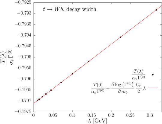
Figure C.2: NLO corrections to the top decay width computed with a finite gluon mass $\lambda$.

C.3 Considerations

We have just seen that both $\sigma(W^{*}\to t\bar{b})$ and $\Gamma\left(t\to W\,b\right)$ are linear-renormalon free if expressed in terms of the $\overline{\rm MS}$ mass, so it is the cross section $\sigma(W^{*}\to t\bar{b}\to W\,b\,\bar{b})$ in NWA. In Sec. 5.1.2 we showed that this behaviour is achieved also for finite top width, since the top quark can never be on-shell if a complex mass scheme is used. A formal demonstration of the cancellation of the linear sensitivity in case of finite top width is given in appendix D.

Appendix D Cancellation of the linear sensitivity in the total cross section and in leptonic observables

In order to discuss the cancellation of the linear sensitivity in the total cross section and in the energy of the $W$ boson, $E_{\mathchoice{\displaystyle}{\scriptstyle}{\scriptscriptstyle}{\scriptscriptstyle}W}$, when finite top-width effects are included, we make use of the old-fashioned perturbation theory. To this purpose, we first briefly summarize the main features of this approach in Appendix D.1 and we recall the conditions for Landau threshold singularities in Appendix D.2. In Appendix D.3 we show that, as long as $\Gamma_{t}>0$, the Landau singularities are not present and thus, if we adopt a short-distance mass, no linear $m_{g}$-term can arise, being $m_{g}$ the mass of the gluon.

D.1 Old-fashioned perturbation theory

In the old-fashioned (time-ordered) perturbation theory the propagator denominators in a Feynman diagram are split into an advanced and a retarded part

$$\frac{i}{k^{2}-m^{2}+i\eta}=\frac{i}{2E_{k,m}}\left[\frac{1}{k^{0}-E_{k,m}+i\eta}+\frac{1}{-k^{0}-E_{k,m}+i\eta}\right],$$ (D.1)

where

$$E_{k,m}=\sqrt{\underline{k}^{2}+m^{2}},$$ (D.2)

and $\underline{k}=|\vec{k}|$. The time Fourier transform of the first term vanishes for negative time, while for the second term it vanishes for positive time

$$\int\frac{\mathrm{d}k^{0}}{2\pi}\frac{i\exp(-ik^{0}t)}{k^{0}-E_{k,m}+i\eta} = \theta(t)\exp\!\left(-iE_{k,m}\,t\right)\,,$$ (D.3)

$$\int\frac{\mathrm{d}k^{0}}{2\pi}\frac{i\exp(-ik^{0}t)}{-k^{0}-E_{k,m}+i\eta} = \theta(-t)\exp\!\left(iE_{k,m}\,t\right)\,.$$ (D.4)

These results can be easily demonstrated by promoting the integration path into a semicircle integral and applying the residue theorem.

We observe that the first term in eq. (D.1), that corresponds to an advanced propagator, propagates positive energies in the future, while the second one, i.e. the retarded one, propagates negative energies in the past.

In presence of an unstable particle, the denominator is given by

$$\frac{i}{k^{2}-m^{2}+im\Gamma}=\frac{i}{2E_{k,m,\Gamma}}\left[\frac{1}{k^{0}-E_{k,m,\Gamma}}+\frac{1}{-k^{0}-E_{k,m,\Gamma}}\right],$$ (D.5)

where

$$E_{k,m,\Gamma}=\sqrt{\underline{k}^{2}+m^{2}-im\Gamma}\,,$$ (D.6)

so that $E_{k,m,\Gamma}$ has a negative imaginary part. As a consequence, we also have

$$\int\frac{\mathrm{d}k^{0}}{2\pi}\frac{i\exp(-ik^{0}t)}{k^{0}-E_{k,m,\Gamma}+i\eta} = \theta(t)\exp\!\left(-iE_{k,m,\Gamma}^{0}\,t\right)\,,$$

$$\int\frac{\mathrm{d}k^{0}}{2\pi}\frac{i\exp(-ik^{0}t)}{-k^{0}-E_{k,m,\Gamma}+i\eta} = \theta(-t)\exp\!\left(iE_{k,m,\Gamma}^{0}\,t\right)\,,$$

and both functions have exponential damping for large positive (negative) time. We notice that the $i\eta$ factor is not necessary in intermediate states containing the unstable particle, because they can never be on-shell.

We can write any Feynman diagram assigning an independent momentum to each propagator, and include a factor $(2\pi)^{4}\delta^{4}\left(\sum k\right)$ to each vertex to ensure four-momentum conservation, where $\sum k$ is the sum of all four-momenta entering the vertex. Furthermore, the time component of the $\delta$ function can be rewritten as

$$(2\pi)^{4}\delta^{4}\left(\sum k\right)=\int_{-\infty}^{+\infty}\mathrm{d}t\exp\left(-it\sum k_{0}\right)\,(2\pi)^{3}\delta^{3}\left(\sum\vec{k}\right).$$ (D.7)

Thus each advanced or retarded propagator will carry the factor

$$\frac{1}{2E_{k,m}}\frac{\exp\!\left[-i(t_{2}-t_{1})k_{0}\right]}{\pm k^{0}-E_{k,m}+i\eta},$$ (D.8)

where $t_{1}$ and $t_{2}$ are the time variables associated with the beginning and the end of the propagator, that are chosen accordingly to the direction of $\vec{k}$. Performing the $k^{0}$ integration, we get

$$\int_{-\infty}^{\infty}\frac{\mathrm{d}k_{0}}{2\pi}\frac{i}{2E_{k,m}}\frac{\exp\!\left[-i(t_{2}-t_{1})k_{0}\right]}{\pm k^{0}-E_{k,m}+i\eta}=\theta(\pm(t_{2}-t_{1}))\exp(\mp iE_{k,m}t)\,\frac{1}{2\,E_{k,m}}\,,$$ (D.9)

with $k^{0}$ replaced by its on shell (positive or negative) value in all other occurrences (i.e. propagator numerators or vertex factors).

By splitting each propagator into an advanced and retarted part, a single Feynman diagram will split into a sum of diagrams with all possible different time orderings for the vertices. We consider a graph with a given ordering, and label the time of each vertex as

$$t_{0}<t_{1}<\ldots<t_{n}\,,$$ (D.10)

and we can collect all exponential in the form

$$\exp(-it_{0}E_{V_{0}})\ldots\exp(-it_{n}E_{V_{n}})\,,$$ (D.11)

where by $E_{V_{i}}$ we mean the total energy entering the $i^{\operatorname{th}}$ vertex. Integrating in $t_{n}$ from $t_{n-1}$ to infinity yields a factor

$$\int_{t_{n-1}}^{+\infty}\mathrm{d}t_{n}\,\exp(-it_{n}E_{V_{n}})=-i\frac{\exp(-it_{n-1}E_{V_{n}})}{E_{V_{n}}-i\eta}.$$ (D.12)

Then, performing the $\mathrm{d}t_{n-1}$ integration yields

$$\frac{-i}{E_{V_{n}}-i\eta}\int_{t_{n-2}}^{+\infty}\mathrm{d}t_{n}\,\exp\left[-it_{n}(E_{V_{n}}+E_{V_{n}-1})\right]=(-i)^{2}\frac{\exp\left[-it_{n-2}(E_{V_{n-1}}+E_{V_{n}})\right]}{(E_{V_{n}}-i\eta)(E_{V_{n-1}}+E_{V_{n}}-i\eta)},$$ (D.13)

and so on. The last integral in $\mathrm{d}t_{0}$ is unrestricted, yielding

$$\frac{(-i)^{n}\,2\pi\,\delta(E_{V_{0}}+E_{V_{1}}+\ldots E_{V_{n}})}{(E_{V_{n}}-i\eta)\ldots(E_{V_{n}}+E_{V_{n-1}}\ldots+E_{V_{1}}-i\eta)},$$ (D.14)

i.e. the total energy entering in all the vertices must be zero. The delta function is usually removed from the amplitude.

In order to have a clearer picture of the resulting graph, we can attach a line coming from $t=-\infty$ to all vertices with an entering external momentum, and a line going to $t=+\infty$ from all vertices with outgoing external momenta. Then we imagine we cut our Feynman graphs with lines at constant time between any pair or time-ordered vertices $i-1,i$. This line defines the intermediate state $S_{i}$. We define the energy of the intermediate state $S_{i}$ as the sum $E_{S_{i}}$ of the energy flowing in all cut lines (including those from $-\infty$ or to $+\infty$) from smaller to larger times. Then, the denominator of the $i^{\operatorname{th}}$ vertex is

$$\frac{i}{E-E_{S_{i}}+i\eta},$$ (D.15)

where $E=E_{S_{-1}}=E_{S_{n+1}}$ is the energy of the intermediate state before all vertices, and the energy of the intermediate state after all vertices, that are equal by momentum conservation. In fact, in general the denominator arising from the $n^{\operatorname{th}}$ vertex is

$$\frac{-i}{E_{V_{n}}-i\eta}.$$ (D.16)

Since $E_{n}$ is the total energy entering the last vertex, it must equal the energy of the $S_{n}$ intermediate state, minus the energy of the $S_{n+1}$ state

$$\frac{-i}{E_{V_{n}}-i\eta}=\frac{-i}{E_{S_{n}}-E-i\eta}=\frac{i}{E-E_{S_{n}}+i\eta}.$$ (D.17)

The denominator arising from the $n-1$ vertex is instead

$$\frac{-i}{E_{V_{n}}+E_{V_{n-1}}-i\eta}.$$ (D.18)

Arguing as before, $E_{V_{n-1}}=E_{S_{n-1}}-E_{S_{n}}$, so

$$\frac{-i}{E_{V_{n}}+E_{V_{n-1}}-i\eta}=\frac{-i}{E_{S_{n}}-E+E_{S_{n-1}}-E_{S_{n}}+i\eta}=\frac{i}{E-E_{S_{n-1}}+i\eta},$$ (D.19)

and so on. Indeed, if we take for example the Feynman diagram of Fig. D.1 and we write the energy entering in each vertex, we have

Figure D.1: Example of time ordered graph.

• $E_{V_{0}}=(E_{-\infty})-(E_{q,1}+E_{\bar{q}})=E_{S_{0}}-E_{S_{1}}=E-E_{S_{1}}$

• $E_{V_{1}}=E_{q,1}-E_{W}-E_{q,2}=(E_{q,1}+E_{\bar{q}})-(E_{W}+E_{q,2}+E_{\bar{q}})=E_{S_{1}}-E_{S_{2}}$;

• $E_{V_{2}}=E_{W}+E_{q,2}-E_{q,3}=(E_{W}+E_{q,2}+E_{\bar{q}})-(E_{q,3}+E_{\bar{q}})=E_{S_{2}}-E_{S_{3}}$;

• $E_{V_{3}}=(E_{q,3}+E_{\bar{q}})-(E_{+\infty})=E_{S_{3}}-E_{S_{4}}=E_{S_{3}}-E$.

We can now formulate the rules for representing a given Feynman graph as the sum of contributions coming from old-fashioned perturbation theory:

1. For a given Feynman graph, consider all possible ordering of its vertices. Write the whole Feynman graph formula without the inclusion of the $i/(k^{2}-m^{2}+i\eta)$ factors.

2. For each line joining two vertices provide the factor

   $$\frac{1}{2E_{k,m}}=\frac{1}{2\sqrt{\underline{k}^{2}+m^{2}}},$$ (D.20)

   where $\underline{k}$ is the modulus of the three-momentum flowing in the graph. Assume that the energy $E_{k,m}$ flowing in propagators from smaller to larger time vertices is positive. This factor indeed multiplies the advanced/retarded propagator in eq. (D.1).

3. In all numerator factors of the Feynman graph, substitute the time component of the momenta flowing in the propagators with its on-shell value, with the sign determined according to the convention of the previous point. This is a consequence of eq. (D.9).

4. Assign 3-momenta as usual, with 3-momentum conservation at each vertex, and

   $$\frac{\mathrm{d}^{3}\vec{k}}{(2\pi)^{3}}$$ (D.21)

   momentum integration.

5. Add lines from $t=-\infty$ to each vertex with entering external momentum.

6. Add lines to $t=\infty$ to each vertex with exiting external momentum.

7. Consider all intermediate states between any pair of nearby vertices. For each intermediate state provide a factor

   $$\frac{i}{E-E_{S_{i}}+i\eta},$$ (D.22)

   where $E$ is the total energy coming from $-\infty$ (or going to $+\infty$) and $E_{S_{i}}$ is the energy of the state $S_{i}$.

Notice that each energy denominator carries a factor of $i$, and so does each vertex. Since the number of energy denominators is equal to the number of vertices minus 1, one $i$ will survive in the product.

D.2 Landau singularities

Landau singularities [100, 101] are naturally explained in the old-fashioned perturbation theory. In general, we have a denominator of the form

$$\frac{1}{E-\sum_{i=1}^{n}\sqrt{|\vec{k}_{i}|^{2}+m_{i}^{2}}+i\eta},\qquad E\sim\sum_{i=1}^{n}m_{i}.$$ (D.23)

The so-called Landau anomalous threshold can arise when a sequel of singular denominators appear at the same time. Let us assume we have a single loop where the 3-momentum $\vec{k}$ flows, and we have a set of denominators

$$\prod_{i=1}^{n}D_{i}=\prod_{i=1}^{n}\frac{1}{E_{i}-\sum_{j_{i}=1}^{n_{i}}\sqrt{(\vec{q}_{j}+\vec{k})^{2}+m_{j}^{2}}+i\eta}.$$ (D.24)

Assuming that the term $E_{i}$ can be different for each denominator amounts to the assumption that we may have external momenta entering at any vertex. We now assume that at some value of $\vec{k}=\vec{k}_{0}$ all denominators vanish at the same time. A necessary and sufficient condition for this to be an avoidable singularity is that upon integrating in any component of $\vec{k}$ all $i\eta$ pole are on the same side of the integration plane near $\vec{k}_{0}$. We expand a energy denominator for $\vec{k}=\vec{k}_{0}+\delta\vec{k}$.

$$D_{i} = \frac{1}{E_{i}-\sum_{j_{i}=1}^{n_{i}}\sqrt{(\vec{q}_{j}+\vec{k}_{0}+\delta\vec{k})^{2}+m_{j}^{2}}+i\eta}$$ (D.25)

$$\approx \frac{1}{E_{i}-\sum_{j_{i}=1}^{n_{i}}\sqrt{(\vec{q}_{j}+\vec{k}_{0})^{2}+m_{j}^{2}}-\delta\vec{k}\cdot\sum_{j=1}^{n_{i}}\frac{\vec{q}_{j}+\vec{k}_{0}}{\sqrt{(\vec{q}_{j}+\vec{k}_{0})^{2}+m_{j}^{2}}}+i\eta}$$

$$= \frac{1}{-\delta\vec{k}\cdot\sum_{j=1}^{n_{i}}\frac{\vec{q}_{j}+\vec{k}_{0}}{\sqrt{(\vec{q}_{j}+\vec{k}_{0})^{2}+m_{j}^{2}}}+i\eta}=\frac{-1}{(\vec{k}-\vec{k_{0}})\cdot\sum_{j=1}^{n_{i}}\frac{\vec{q}_{j}\vec{k}_{0}}{\sqrt{(\vec{q}_{j}+\vec{k}_{0})^{2}+m_{j}^{2}}}-i\eta}.\qquad$$

In one dimension the sign of the imaginary part of the complex pole is given by

$$-{\rm sign}\left(\sum_{j=1}^{n_{i}}\frac{q_{j}+k_{0}}{\sqrt{({q}_{j}+{k}_{0})^{2}+m_{j}^{2}}}\right)\,,$$ (D.26)

so, if this sum has the same sign for all the $D_{i}$, the singularity is avoidable since it lies in the same part of the complex plane for all the denominators. In 3 dimensions, if there is a direction in the 3-dimensional integration space (corresponding to the 3-momenta flowing in the loop) such that, integrating along it, it leaves the singularities of all the $D_{i}$ on the same side of the complex plane, the integration contour can be deformed away from the singularity, so that the denominators cannot contribute to the singularities. This is achieved if there is at least one direction of $\delta\vec{k}$ such that

$$\delta\vec{k}\cdot\sum_{j=1}^{n_{i}}\frac{\vec{q}_{j}+\vec{k}_{0}}{\sqrt{(\vec{q}_{j}+\vec{k}_{0})^{2}+m_{j}^{2}}}$$ (D.27)

have the same sign for all $i$. Thus, all vectors given by the sum in (D.27) have components of the same sign in at least one direction and so no null linear combination

$$\sum_{i=1}^{n}\lambda_{i}\sum_{j=1}^{n_{i}}\frac{\vec{q}_{j}+\vec{k}_{0}}{\sqrt{(\vec{q}_{j}+\vec{k}_{0})^{2}+m_{j}^{2}}}=0$$ (D.28)

must exist for any sequence of $\lambda_{i}>0$. Conversely, if a null linear combination exists, (D.27) cannot be satisfied for any choice of $\delta\vec{k}$. This is the so-called Landau anomalous threshold singularity.

The physical interpretation of eq. (D.28) is quite interesting. We interpret the $\lambda_{i}$ as the time between the first vertex on the left and on the right of the $i^{\operatorname{th}}$ intermediate state. The ratios in the sum in (D.28) are just the velocities of the particles, so, velocities times time equal the displacements. So, the sum of all displacements of internal particles must be zero. Since all internal particles are nearly on-shell (i.e. their displacement can be as large as one likes), this means that their displacements must be compatible with kinematic constraints. This is better illustrated with the example of Fig. D.2.

Figure D.2: Illustration of eq. (D.28).

The condition for the singularity is

$$\left(\vec{v}_{1}+\vec{v}_{2}\right)\lambda_{1}+\left(\vec{v}_{3}+\vec{v}_{2}\right)\lambda_{2}+\left(\vec{v}_{3}+\vec{v}_{4}\right)\lambda_{3}=0,\qquad\mbox{with }\;\vec{v}_{i}=\frac{\vec{k}_{i}}{\sqrt{|\vec{k}_{i}|^{2}+m_{i}^{2}}}\,,$$ (D.29)

for positive $\lambda_{1\ldots 3}$. This is the same as

$$\vec{v}_{1}\lambda_{1}+\vec{v}_{3}(\lambda_{3}+\lambda_{2})=-\vec{v}_{2}(\lambda_{1}+\lambda_{2})-\vec{v}_{4}\lambda_{3},$$ (D.30)

i.e. the displacement of particle 1 between its initial and final vertex, plus the displacement of particle 3 between its initial and final vertex is equal and opposite to the subsequent displacement of particles 2 and 4. In other words, the momenta should be such that the particles meet again after having come apart.

D.3 The specific case

We now consider our $W^{\ast}\rightarrow\bar{b}+(t\rightarrow W+b)$ process. An example of NLO diagram is shown in Fig. D.3.

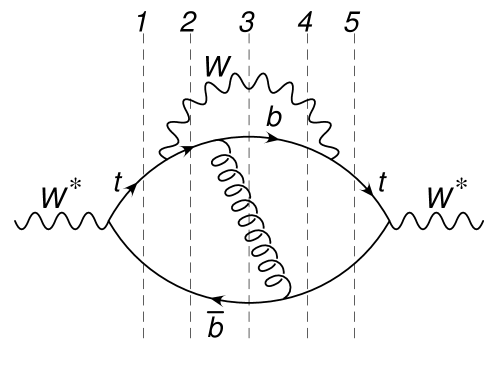
Figure D.3: Example of NLO contribution to the process $W^{\ast}\rightarrow t\bar{b}\rightarrow Wb\bar{b}$.

The corresponding contribution to the cross section is obtained by setting either one of the 2, 3, 4 intermediate states on the energy shell, and changing the sign of the $i\eta$ in the denominators to the right of the cut. We then define

$$D_{1} = \frac{1}{E-E_{t,1}-E_{\bar{b},1}}\,,$$ (D.31)

$$D_{2} = \frac{1}{E-E_{\mathchoice{\displaystyle}{\scriptstyle}{\scriptscriptstyle}{\scriptscriptstyle}W}-E_{b,2}-E_{\bar{b},1}+i\eta}\,,$$ (D.32)

$$D_{3} = \frac{1}{E-E_{\mathchoice{\displaystyle}{\scriptstyle}{\scriptscriptstyle}{\scriptscriptstyle}W}-E_{b,3}-E_{\bar{b},1}-E_{g,3}+i\eta}\,,$$ (D.33)

$$D_{4} = \frac{1}{E-E_{\mathchoice{\displaystyle}{\scriptstyle}{\scriptscriptstyle}{\scriptscriptstyle}W}-E_{b,3}-E_{\bar{b},4}+i\eta}\,,$$ (D.34)

$$D_{5} = \frac{1}{E-E_{t,5}-E_{\bar{b},5}}\,,$$ (D.35)

where

$$E_{t,i} = \sqrt{\vec{k}_{t,i}^{2}+m^{2}-im\Gamma_{t}}\,,$$ (D.36)

$$E_{l,i} = \sqrt{\vec{k}_{l,i}^{2}}\,,\qquad\qquad l=b,\bar{b},g,\,$$ (D.37)

$$E_{\mathchoice{\displaystyle}{\scriptstyle}{\scriptscriptstyle}{\scriptscriptstyle}W} = \sqrt{\vec{k}_{\mathchoice{\displaystyle}{\scriptstyle}{\scriptscriptstyle}{\scriptscriptstyle}W}^{2}+m^{2}}\,.$$ (D.38)

Notice that the top energy has an imaginary part, so that no $i\eta$ is needed in the denominators containing it. We never include the corresponding cuts since the top width prevents this particle from being on-shell. Thus, the only intermediate states contributing to cuts will be the ones that do not include the top. According to the optical theorem, the cross section is given by the imaginary part of a sum of contributions like the one displayed in Fig. D.3. Since we do not include contributions in which the top is on-shell, in the integrand for the cross section we have

$$D_{1}\,\operatorname{Im}[D_{2}D_{3}D_{4}]D_{5}^{*}=D_{1}\big{[}{\rm Im}(D_{2})D_{3}^{*}\,D_{4}^{*}+D_{2}\,{\rm Im}(D_{3})D_{4}^{*}+D_{2}\,D_{3}\,{\rm Im}(D_{4})\big{]}D_{5}^{*}\,.$$ (D.39)

When performing the 3-momentum integral for the loops not including the $W$ line, one can come close to the singularity in the denominators. However, if there is a direction in the 9-dimensional integration space (corresponding to the three 3-momenta flowing in the loops) such that, integrating along it, it leaves the singularities of $D_{2}$, $D_{3}$ and $D_{4}$ on the same side of the complex plane, the integration contour can be deformed away from the singularities, so that the denominators cannot contribute to mass singularities. The singularity for small $\lambda$ will thus be determined only by the remaining factor

$$\frac{\mathrm{d}^{3}k_{g}}{\sqrt{\vec{k}_{g}^{2}+\lambda^{2}}}\,,$$ (D.40)

that gives a quadratic sensitivity to the gluon mass $\lambda$.

As we have already discussed, the only cases when an appropriate deformation of the contour does not exist correspond to Landau singularities.

In order to explore the possible Landau configuration, one can start with the graph of Fig. D.3 with the top lines shrunk to a point. In fact, the top is always off-shell, and it cannot propagate over large distances. The remaining configuration is shown in Fig. D.4.

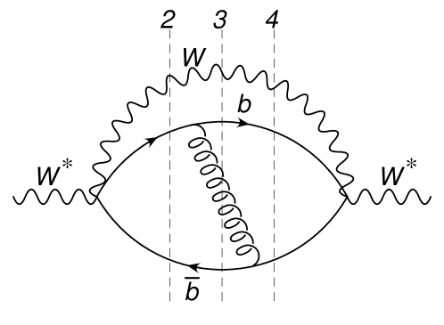
Figure D.4: The reduced graph to look for Landau singularities in the graph of Fig. D.3.

In order for the 2, 3 and 4 intermediate states to be on-shell at the same time, either both the $b$ and the $\bar{b}$ are collinear to the gluon, or the gluon is soft. In the first case, also the two $b$ quarks and the gluon are collinear, and are all travelling in the opposite direction with respect to the $W$. Thus, they cannot meet at the same point on the last vertex to the right. On the other hand, if the gluon is soft, the $b$, the $\bar{b}$ and the $W$ produced at the primary vertex have momenta that sum to zero, so, again their velocities will make them diverge. In both cases eq. (D.28) cannot be satisfied and these configurations lead to an avoidable singularity. One can try to shrink other propagators to a point to see if two intermediate states can be on-shell. Shrinking a $b$ and a $\bar{b}$ line to a point leads to configuration with two massless system (either $b$ quarks of collinear $bg$ systems) and a $W$, that again cannot meet at the same point. Shrinking the $W$, the two $b$ or the two $\bar{b}$ lines to a point shrinks the whole graph to a point, leading to nothing. Thus, no Landau configuration can exist, so one infers that the $m_{g}$ sensitivity of the total cross section is at least quadratic.

We can repeat the same reasoning including a factor $E_{\mathchoice{\displaystyle}{\scriptstyle}{\scriptscriptstyle}{\scriptscriptstyle}W}$ in our Feynman graph. The argument runs as before, and so even for the average energy of the $W$ one expects that the sensitivity to the gluon mass is at least quadratic. Notice that in order for this to work, one needs that the $E_{\mathchoice{\displaystyle}{\scriptstyle}{\scriptscriptstyle}{\scriptscriptstyle}W}$ factor is the same for all cuts, which is in fact the case.

This argument fails if $\Gamma_{t}$ is sent to zero. Indeed in this case $D_{1}$ and $D_{5}^{*}$ can be simultaneously singular but their $i\eta$ have opposite signs. Under these condition, the pinch is clearly unavoidable.

As a last point, we recall that the total cross section is free of linear $m_{g}$ sensitivity also in the limit of zero width. This happens because, in the zero-width limit, the cross section factorizes into a production cross section times a decay width, and both of them are free of linear sensitivity to $m_{g}$ if the mass is in a short-distance scheme. The same, however, does not hold for the average $E_{\mathchoice{\displaystyle}{\scriptstyle}{\scriptscriptstyle}{\scriptscriptstyle}W}$. In fact, the cancellation of mass singularities in $\Gamma_{t}$ cannot be proven in the same fashioned adopted here, since logarithmic divergences are also present in the wave-function renormalization, and cannot be treated in a straightforward way in the old-fashioned perturbation theory.

Appendix E The POWHEG BOX framework

The fixed order computations needed to evaluate the factors $T(\lambda)$ and $\widetilde{T}(\lambda)$ of eqs. (4.45) and (4.64) and the NLO generators described in chap. 9 are implemented in the POWHEG BOX. The POWHEG BOX is a framework that can be used to generate NLO events that can be interfaced to modern parton shower (PS) according to the POWHEG method [98, 102, 103]. The latest release, i.e. the POWHEG BOX RES [38], has been developed to handle processes containing coloured resonances that can emit.

E.1 NLO computations in the POWHEG BOX (RES)

The POWHEG BOX can be used as an integrator for fixed order NLO computations. The user has to provide, according to Ref. [103]:

• the Born squared amplitude;

• the finite part of the virtual squared amplitude;

• the real squared amplitude;

• the Born phase space (in the POWHEG BOX RES it can be generated automatically);

• the flavour structure of the Born and of the real processes;

• the Born colour- and spin-correlated squared amplitudes.

We describe the main features for the computations of a $2\to n$ process at NLO for a generic hadron-hadron collision. We introduce $\mathbb{\Phi}_{n}$ to be the set of variables

$$\mathbb{\Phi}_{n}=\left\{x_{1},x_{2},p_{1},\dots p_{n}\right\},$$ (E.1)

being $x_{1,2}$ the fractions of the hadrons energies carried by the incoming partons and $p_{1},\dots,p_{n}$ the four-momenta of the outgoing particles. We define the luminosity $\mathcal{L}=f_{1}^{i}(x_{1})f_{2}^{j}(x_{2})$, where $f_{1}^{i}(x_{1})$ is the parton distribution function relative to the first hadron and it describes the probability of finding a parton $i$ carrying a fraction $x_{1}$ of the hadron energy. If one of the incoming particle is a lepton, we replace $f_{1}^{i}(x_{1})$ with $\delta(x_{1}-1)$. We also denote with $\mathcal{B}$ the partonic Born cross section, with $\mathcal{V}_{\rm b}$ the partonic UV-renormalized virtual cross section and with $\mathcal{R}$ the partonic real cross section. The total NLO cross section is given by

$$\sigma^{\rm NLO} = \int\mathrm{d}\mathbb{\Phi}_{n}\;\mathcal{L}\left[\mathcal{B}(\mathbb{\Phi}_{n})+\mathcal{V}_{\rm b}(\mathbb{\Phi}_{n})\right]+\int\mathrm{d}\mathbb{\Phi}_{n+1}\;\mathcal{L}\;\mathcal{R}(\mathbb{\Phi}_{n+1})$$

$$+\sum_{i=1}^{2}\int\mathrm{d}\mathbb{\Phi}_{n}\int_{0}^{1}\mathrm{d}{z}\;\mathcal{L}\;\mathcal{G}_{i}(z,\mathbb{\Phi}_{n})\,,$$

where the $\mathcal{G}_{i}$ terms are introduced by the renormalization of $\mathcal{L}$ and they ensure the cancellation of the initial-state collinear singularities contained in $\mathcal{R}$. If the incoming particle $i$ is a lepton, $\mathcal{G}_{i}=0$. For ease of notation, we define

$$\mathcal{V}(\mathbb{\Phi}_{n})=\mathcal{V}_{\rm b}(\mathbb{\Phi}_{n})+\sum_{i=1}^{2}\int_{0}^{1}\mathrm{d}{z}\;\mathcal{G}_{i}(z,\mathbb{\Phi}_{n}).$$ (E.3)

The Kinoshita-Lee-Nauenberg (KLN) [104, 105] theorem guarantees us that the infrared divergences contained in $\mathcal{R}$ and in $\mathcal{V}$ cancel, yielding to a finite prediction for $\sigma^{\rm NLO}$.

In order to handle numerically eq. (E.1), a counterterm $\mathcal{C}(\mathbb{\Phi}_{\rm n+1})$ is introduced, that approaches the real cross section in the soft and collinear limit, such as $\mathcal{R}(\mathbb{\Phi}_{\rm n+1})-\mathcal{C}(\mathbb{\Phi}_{\rm n+1})$ is finite. The phase space $\mathbb{\Phi}_{\rm n+1}$ can be rewritten as

$$\mathbb{\Phi}_{\rm n+1}=\left\{\mathbb{\Phi}_{n},\Phi_{\rm rad}\right\}\,,$$ (E.4)

where $\mathbb{\Phi}_{n}$ is the phase space of the underlying Born configuration and $\Phi_{\rm rad}$ is a set of 3 kinematic variables that describe the phase space of the extra parton emitted in the $n+1$-body configuration. The total cross section now takes the form

$$\sigma^{\rm NLO} = \int\mathrm{d}\mathbb{\Phi}_{n}\;\mathcal{L}\;\mathcal{B}(\mathbb{\Phi}_{n})+\int\mathrm{d}\mathbb{\Phi}_{n}\;\mathcal{L}\left[\mathcal{V}(\mathbb{\Phi}_{n})+\int\mathrm{d}\Phi_{\rm rad}\;\mathcal{C}(\mathbb{\Phi}_{n+1})\right]$$

$$+\int\mathrm{d}\mathbb{\Phi}_{n+1}\;\mathcal{L}\left[\mathcal{R}(\mathbb{\Phi}_{n+1})-\mathcal{C}(\mathbb{\Phi}_{n+1})\right]\,,$$

where the expression in the squared brackets is finite in $d=4$ dimensions and thus can be evaluated numerically.

With this subtraction formalism, we can compute predictions for any generic infrared-safe observable $O$, i.e. such that $O_{n+1}(\mathbb{\Phi}_{n+1})\to O_{n}(\mathbb{\Phi}_{n})$ when one parton becomes soft or collinear to another one. More explicitly, we have

$$O = \int\mathrm{d}\mathbb{\Phi}_{n}\;\mathcal{L}\;\mathcal{B}(\mathbb{\Phi}_{n})\;O_{n}(\mathbb{\Phi}_{n})$$

$$+\int\mathrm{d}\mathbb{\Phi}_{n}\;\mathcal{L}\left[\mathcal{V}(\mathbb{\Phi}_{n})+\int\mathrm{d}\Phi_{\rm rad}\;\mathcal{C}(\mathbb{\Phi}_{n+1})\right]O_{n}(\mathbb{\Phi}_{n})$$

$$+\int\mathrm{d}\mathbb{\Phi}_{n+1}\;\mathcal{L}\left[\mathcal{R}(\mathbb{\Phi}_{n+1})\;O_{n+1}(\mathbb{\Phi}_{n+1})-\mathcal{C}(\mathbb{\Phi}_{n+1})\;O_{n}(\mathbb{\Phi}_{n})\right]\,.$$

In the POWHEG BOX framework, the counterterms $\mathcal{C}$ introduced eq. (E.1) is evaluated using the Frixione-Kunszt-Signer (FKS) subtraction [78] method. The real cross section is written as a sum of terms, each of them containing at most one collinear and one soft singularity associated with one parton (the FKS parton). We label with $i$ the region of the phase space where the parton $i$ becomes soft or collinear to an incoming parton, $ij$ the region where $i$ and $j$ are collinear. We introduce non-negative functions $d_{i}$ and $d_{ij}$, that in the POWHEG BOX are defined as

$$d_{i}=E^{2}_{i}(1-\cos^{2}\theta_{i})\,,\qquad d_{ij}=\frac{2\,E_{i}\,E_{j}}{(E_{i}+E_{j})^{2}}\,p_{i}\cdot p_{j}\,,$$ (E.7)

being $E_{i}$ and $p_{i}$ the energies and the four-momenta of the parton $i$, $\theta_{i}$ the angle between the parton $i$ and the beams axis, everything computed in the partonic rest frame. This enables us to introduce the $\mathcal{S}$ functions defined as

$$\mathcal{S}_{i}=\frac{1}{d_{i}\;\mathcal{D}}\,,\qquad\mathcal{S}_{ij}=\frac{1}{d_{ij}\;\mathcal{D}}.$$ (E.8)

where

$$\mathcal{D}=\sum_{i}\frac{1}{d_{i}}+\sum_{ij}\frac{1}{d_{ij}}\,.$$ (E.9)

The real cross section $\mathcal{R}$ is then split into a sum of contributions associated to the several singular regions:

$$\mathcal{R}=\sum_{i}\mathcal{R}_{i}+\sum_{ij}\mathcal{R}_{ij}\,,$$ (E.10)

with

$$\mathcal{R}_{i}=\mathcal{S}_{i}\mathcal{R}\,,\qquad\mathcal{R}_{ij}=\mathcal{S}_{ij}\mathcal{R}.$$ (E.11)

This decomposition offers us the possibility to choose a different parametrization for the $n+1$-body phase space for each contribution $\alpha=i,ij$.

$$\int\mathrm{d}\mathbb{\Phi}_{n+1}\;\mathcal{L}\left[\mathcal{R}(\mathbb{\Phi}_{n+1})-\mathcal{C}(\mathbb{\Phi}_{n+1})\right]=\sum_{\alpha}\int\mathrm{d}\mathbb{\Phi}^{\alpha}_{n+1}\;\mathcal{L}\left[\mathcal{R}^{\alpha}(\mathbb{\Phi}^{\alpha}_{n+1})-\mathcal{C}^{\alpha}(\mathbb{\Phi}^{\alpha}_{n+1})\right].$$ (E.12)

A fully detailed description of this method can be found in Ref. [102]. What we want to underline is that for each region $\alpha$, we have a subtraction term $\mathcal{C}^{\alpha}$, that approaches $\mathcal{R}^{\alpha}$ when $\alpha$ is singular. The subtraction terms $\mathcal{C}^{\alpha}$ are automatically built by POWHEG BOX from the Born squared amplitude

$$\mathcal{C}^{\alpha}(\mathbb{\Phi}^{\alpha}_{n+1})=\tilde{\mathcal{C}}(\mathbb{\Phi}^{\alpha}_{n},\Phi_{\rm rad})\;\;\mathcal{B}^{\alpha}(\mathbb{\Phi}^{\alpha}_{n})\,$$ (E.13)

and $\tilde{\mathcal{C}}(\mathbb{\Phi}^{\alpha}_{n},\Phi^{\rm\alpha}_{\rm rad})$ is a function that can be easily integrated analytically in $d=4-2\epsilon$ dimensions over the radiation phase space. The underlying Born phase space $\mathbb{\Phi}^{\alpha}_{n}$ associated with $\mathbb{\Phi}^{\alpha}_{n+1}$ is reconstructed using a mapping $M_{\alpha}(\mathbb{\Phi}^{\alpha}_{n+1})$. When the parton $i$ is soft or collinear to the parton $j$, $M_{\alpha}(\mathbb{\Phi}^{\alpha}_{n+1})$ should fulfill the following property:

$$\mathbb{\Phi}^{\alpha}_{n+1}=\left\{x_{1},x_{2},\dots,p_{i},p_{j},\dots\right\}\to\mathbb{\Phi}^{\alpha}_{n}=\left\{x^{\prime}_{1},x^{\prime}_{2},\dots,p_{i}+p_{j},\dots\right\},$$ (E.14)

where the incoming partons energy-fraction differs in case of an initial-state emission. The inverse mapping $M^{-1}_{\alpha}(\mathbb{\Phi}^{\alpha}_{n+1})$ is used to generate the real emission phase space from $\mathbb{\Phi}^{\alpha}_{n}$ and the three radiation variables.

From eq. (E.13) we see that the subtraction term is proportional to the Born and thus it will contains the denominators like $(p^{2}-m^{2})^{2}+\Gamma^{2}m^{2}$, being $m$ and $\Gamma$ the pole mass and the decay width of resonance and $p^{2}$ its virtuality obtained from the momenta of its decay products as computed in the $n$-body kinematic, while $\mathcal{R}^{\alpha}$ contains the same denominators but evaluated using the full $n+1$-body kinematic. In the collinear limit, the momenta of the underlying Born configurations are assigned by merging the two collinear partons and then applying some reshuffling to ensure that all the external particles are on their mass shell. The procedure described in Sec. 5 of Ref. [102] does not preserve $p^{2}$ and the resonance momentum will differ of an amount of order $m^{2}/E$, being $E$ the energy of the resonance. As it is shown in Ref. [38], the cancellation of the divergences contained in $\mathcal{R}^{\alpha}$ and in $\mathcal{C}^{\alpha}$ takes place only if $m^{2}<\Gamma\;E$. We clearly see that for small decay width the convergence is problematic, and it is completely spoiled in the zero-width limit.

To this purpose, a new version of the POWHEG BOX, namely the POWHEG BOX RES [38], has been built. Given a flavour structure all the possible intermediate resonances histories are assigned. The mapping between the real phase space and the underlying Born configuration preserves the virtuality of the assigned intermediate resonances.

A similar procedure, applied to the dipole subtraction formalism, is described in Ref. [79].

E.2 NLO events with the POWHEG method

The POWHEG method, proposed for the first time in Ref. [98], enables to consistently match NLO computations with PS algorithms.

In order to preserve the NLO accuracy of inclusive observables, the events generated according to the POWHEG method have weight

$$\overline{B}(\mathbb{\Phi}_{n})=B(\mathbb{\Phi}_{n})+V(\mathbb{\Phi}_{n})+\int\mathrm{d}\Phi_{\rm rad}\,R(\mathbb{\Phi}_{n+1})\,,$$ (E.15)

where we have introduced

$$B=\mathcal{L\,B}\,,\qquad V=\mathcal{L\,V}\,,\qquad R=\mathcal{L\,R}\,.$$ (E.16)

The Sudakov form factor, that describes the non-emission probability, is defined by

$$\Delta\big{(}p_{\perp},\mathbb{\Phi}_{n}\big{)}=\prod_{\alpha}\Delta_{\alpha}\big{(}p_{\perp},\mathbb{\Phi}_{n}\big{)}$$ (E.17)

with

$$\Delta_{\alpha}\big{(}p_{\perp},\mathbb{\Phi}_{n}\big{)}=\exp\left\{\frac{-\left[\int\mathrm{d}\Phi^{\alpha}_{\rm rad}\,R^{\alpha}(\mathbb{\Phi}^{\alpha}_{n+1})\,\theta\big{(}p_{\perp}-k_{\perp}(\mathbb{\Phi}^{\alpha}_{n+1})\big{)}\right]_{\mathbb{\Phi}^{\alpha}_{n}=\mathbb{\Phi}_{n}}}{B(\mathbb{\Phi}_{n})}\right\},\qquad$$ (E.18)

with $R^{\alpha}=\mathcal{L\,R}^{\alpha}$ and the hardness of the emission $p_{\perp}$ is defined to be the transverse momentum of the emitted parton with respect to the emitter. Thus, the differential cross section for the first emission becomes

$$\mathrm{d}\sigma=\overline{B}(\mathbb{\Phi}_{n})\;\mathrm{d}\mathbb{\Phi}_{n}\Big{[}\Delta(p_{\perp,\rm min},\mathbb{\Phi}_{n})+\frac{R(\mathbb{\Phi}_{n+1})}{B(\mathbb{\Phi}_{n})}\Delta\big{(}p_{\perp}(\mathbb{\Phi}_{n+1}),\mathbb{\Phi}_{n}\big{)}\;\mathrm{d}\Phi_{\rm rad}\;\Big{]}\,.$$ (E.19)

The event generated by POWHEG BOX using eq. (E.19) is then completed by a standard shower MC program, like Pythia or Herwig. The core of a shower MC is represented by the PS that generates the subsequent emissions in the collinear limit. In order not to spoil the NLO accuracy of the result, a veto algorithm is implemented in such a way that all the emissions with a transverse momentum larger that the POWHEG one are discarded. Further details are given in appendix E.3. The SMC provides also a model for the underlying event, that is generally described in terms of multiple-parton interactions (MPI), and for the hadronization. The POWHEG BOX framework offers the possibility to separate the real contribution $R$ in two pieces, one containing all the infrared singularities and one finite for $p_{\perp}\to 0$

$$R=R_{s}+R_{f}$$ (E.20)

with

$$R_{s}=\frac{h^{2}}{p_{\perp}^{2}+h^{2}}R\,,\quad R_{f}=\frac{p_{\perp}^{2}}{p_{\perp}^{2}+h^{2}}R\,,$$ (E.21)

where the parameter $h$ is called hdamp in the POWHEG jargon. Only $R_{s}$ is used in the computation of eq. (E.19), while the $R_{f}$ contribution, that corresponds to high transverse momentum radiation, is evaluated separately and it is employed to generate Born-like events called remnants. It is also possible to have a process that admits real corrections that are not associated with any singular region. Those contributions are handled separately in an analogous way to the remnants. The POWHEG formula thus becomes

$$\mathrm{d}\sigma = \overline{B}(\mathbb{\Phi}_{n})\;\mathrm{d}\mathbb{\Phi}_{n}\Big{[}\Delta(p_{\perp,\rm min},\mathbb{\Phi}_{n})+\frac{R_{s}(\mathbb{\Phi}_{n+1})}{B(\mathbb{\Phi}_{n})}\Delta\big{(}p_{\perp}(\mathbb{\Phi}_{n+1}),\mathbb{\Phi}_{n}\big{)}\;\mathrm{d}\Phi_{\rm rad}\;\Big{]}$$ (E.22)

$$+R_{f}(\mathbb{\Phi}_{n+1})\,\mathrm{d}\mathbb{\Phi}_{n+1}\,,$$

where $\overline{B}$ and $\Delta$ are evaluated only using $R_{s}$ and $R_{f}$ collects the either the remnants or the finite real processes.

In the standard POWHEG formalism, radiation is generated using the Sudakov form factor defined in eq. E.17 and it contains the ratio $R(\mathbb{\Phi}_{n+1})/B(\mathbb{\Phi}_{n})$. If the resonance virtualities are not the same when building the underlying Born phase space, large ratios that badly violate the collinear approximation can arise. The improved version of the FKS method implemented in POWHEG BOX RES overcomes this problem.

Furthermore, the PS that will complete the event should be instructed to preserve the mass of the resonances. In the POWHEG BOX RES framework this is achieved by providing a resonance assignment to radiation.

To each Born configuration a resonance structure $f_{b}$ is assigned. The only contribution $\alpha$ we consider are those where the collinear partons both arises from the same resonance (the production process is considered as a resonance). We label with $i$ all the resonances contained in $f_{b}$ and we denote by $\alpha_{i}$ a singular contribution where an emission is originated from the decay products of $i$. The improved resonance-aware POWHEG formalism allow us to write

$$\mathrm{d}\sigma = \sum_{f_{b}}\overline{B}_{f_{b}}(\mathbb{\Phi}_{n})\;\mathrm{d}\mathbb{\Phi}_{n}\prod_{i\in f_{b}}\Bigg{[}\Delta_{i}(p_{\perp,\rm min})$$ (E.23)

$$+\Delta_{i}\left(p_{\perp}(\mathbb{\Phi}_{n+1}),\mathbb{\Phi}_{n}\right)\sum_{\alpha_{i}}\frac{\left[R_{\alpha_{i}}(\mathbb{\Phi}^{\alpha_{i}}_{n+1})\;\mathrm{d}\Phi^{\alpha_{i}}_{\rm rad}\right]_{\mathbb{\Phi}^{\alpha_{i}}_{n}=\mathbb{\Phi}_{n}}}{B_{f_{b}}(\mathbb{\Phi}_{n})}\Bigg{]}\,.$$

Radiation is now generated according to the POWHEG Sudakov form factor both for the production and for all resonance decays that involve coloured partons. This feature also offers the opportunity to modify the standard POWHEG single-radiation approach: instead of keeping only hardest radiation from one of all possible origins, the POWHEG BOX RES can generate simultaneously the hardest radiation in production and in each resonance decay. The Les Houches (LH) events can thus contain more radiated partons, one for production and one for each resonance.

Multiple-radiation events have to be completed by a shower MC program, that has to generate radiation from each origin without exceeding the hardness of the corresponding POWHEG one, thus requiring an interface that goes beyond the simple Les Houches standard [106]. The two most widely used PS programs, Pythia and Herwig, already implement a veto algorithm for radiation in production in order to guarantee that the POWHEG emission is the hardest, while radiation in decay is left, by default, unrestricted.

E.3 NLO+PS matching

We briefly describe now how the NLO events generated with POWHEG BOX (RES) can be completed by the shower MC programs Pythia8.2 or Herwig7.1.

E.3.1 Interface to shower generators

According to the POWHEG method, the event needs to be completed by a standard shower MC program. The subsequent emissions included by the PS must be softer than the POWHEG generated one. In the standard Les Houches Interface for User Processes (LHIUP) [106], each generated event has a hardness parameter associated with it, called scalup. The POWHEG BOX sets this parameter is set equal to the relative transverse momentum of the generated radiation $p_{\perp}$. By default, radiation in decay is left unrestricted and the starting scale is set to be of the order of the resonance virtuality. The PS preserves the virtuality of the resonance, like the POWHEG BOX RES does when generating the real emission, if its decay products have the resonance as mother particle in the LH event record.

A generic method for interfacing POWHEG processes that include radiation in decaying resonances with PS generators was introduced in Refs. [90] and [91]: radiation from the top decay products is left unrestricted and when the event is completed. A veto is applied a posteriori: if any radiation in the decaying resonance shower is found to be harder than the POWHEG generated one, the event is showered again.

The practical implementation of the veto procedure depends on whether we are using a dipole, as in Pythia8.2, or an angular-ordered shower, as in Herwig7.1. In the following we describe the implementation of our veto procedures. Conversely to the method introduced in Ref. [90], we do not need the whole event to be completed before applying the veto, thus saving a lot of computational time.

E.3.2 Pythia8.2

The Pythia8.2 [82] code implements a $p_{\perp}$ ordered shower. Thus, the matching with POWHEG BOX is natural because it is enough to require that the starting scale of the shower evolution is scalup, i.e. the transverse momentum of the POWHEG emission coming from the production process.

When multiple emissions are concerned, the user can define a starting scale for each resonance, implementing the virtual functions canSetResonanceScale and scaleResonance. In this way also emissions from a resonance can have an upper limit defined by the corresponding POWHEG emission, like it is done by default for radiation from the production process. This solution was adopted for example in Ref. [91].

However, the $p_{\perp}$ definitions employed by Pythia and by the POWHEG BOX are slightly different. To overcome this issue, the Pythia8.2 program offers the possibility to use the PowhegHooks class. Each time an emission takes place, its transverse momentum is re-computed with the POWHEG BOX definition: if it is higher than scalup, the emission is discarded.

We have implemented a new class, PowhegHooksBB4L, that can be used for the case of $t\bar{t}$ production and decay. We rewrote the FSREmission method to guarantee that when an emission is originated from the production process, the PowhegHooks machinery can be employed, otherwise, when it comes from the $t$ (or the $\bar{t}$) the momenta of the emitter and of the emitted particles $i$ and $j$ are boosted in the top frame and the transverse momentum of the radiation is computed using

$$p^{2}_{\perp}=2p_{b}\cdot p_{g}\frac{E_{g}}{E_{b}}\,,$$ (E.24)

if the emitter is a $b$ (or $\bar{b}$) heavy quark, using

$$p^{2}_{\perp}=2p_{i}\cdot p_{j}\frac{E_{i}E_{j}}{(E_{i}+E_{j})^{2}}\,,$$ (E.25)

otherwise. If it is harder than the corresponding POWHEG one, this emission is discarded. The FSREmission veto algorithm represents our default choice for handling radiation in decay.

E.3.3 Herwig7.1

The Herwig7.1 package [83, 84] implements an angular ordered PS. In the collinear limit, the variable $q$ that parametrizes the hardness of the emission is given by

$$q\approx E\theta\,,$$ (E.26)

with $E$ the energy of the emitter before the emission and $\theta$ the angle between the two emitted particles. A brief sketch of the evolution of an angular ordered PS is represented graphically in Fig. E.1. The initial stages are characterized by large-angle soft radiation (green), while the hardest emission, i.e. the one with largest $p_{\perp}$ (red), may appear later.

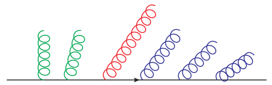
Figure E.1: Angular ordered PS: in green the truncated-vetoed shower, in red the hardest emission and in blue the remaining vetoed shower.

The procedure on how POWHEG-style NLO emissions can be matched with an angular ordered shower is discussed in detail in Ref. [98]. Here we give only a brief summary. The hardest emission originated from a parton $i$ satisfies the following properties:

• it can be found by following the hardest line each time a branching takes place;

• if $i$ is a gluon, the probability that the hardest emission takes place after a $g\to q\bar{q}$ can be neglected, since this splitting is not soft-singular;

• if $i$ is a quark, following the hardest line coincides with following the quark line since the probability that a gluon carries the main part of the energy after a $q\to qg$ splitting is power suppressed.

When matching an event generated with POWHEG BOX with an angular ordered PS, the scale $q$ of the POWHEG emission should be computed. The two partons corresponding to the POWHEG emission should be merged and an angular ordered PS associated with the paired parton, starting from $q_{0}$, the maximum allowed scale, down to $q$, should be implemented. All the emissions with a transverse momentum larger than scalup, i.e. the $p_{\perp}$ of the POWHEG emission, must be vetoed. This shower is called truncated-vetoed shower and corresponds to the green contribution portrayed in Fig E.1. When the scale $q$ is reached, all the subsequent vetoed showers (blue emissions in Fig. E.1) are implemented. Since truncated-vetoed showers are known to give rise only to a little contribution, Herwig7.1 neglects them by default, simply requiring that all the emissions have a transverse momentum smaller than scalup.

However, by doing so, all the large angle emissions with a scale larger than $q$ would be missing. The veto technique introduced in Ref. [99] and activated in Herwig7.1 with the settings

$$\begin{split}&\mbox{\tt set PartnerFinder:PartnerMethod Maximum}\\ &\mbox{\tt set PartnerFinder:ScaleChoice Different}\end{split}$$ (E.27)

performs a task equivalent to the implementation of truncated showers. For example if a $q\to qg$ splitting is the POWHEG hardest emission, the initial angle for radiation from the gluon is taken as the maximum angle between the gluon and its two colour partners, i.e. the incoming and the outgoing quark $q$. This leads to unrestricted radiation from the gluon. However, the colour factor $C_{A}$ associated with this radiation is reduced by a factor of two if the scale of the emission $t^{\prime}$ is larger than the POWHEG one $t$, while it is restored to $C_{A}$ for smaller angles. Since $C_{A}/2\approx C_{F}$ in the large $N_{c}$ limit, we see that this is equivalent to the inclusion of a truncated-vetoed shower from the incoming $q$ quark down to a scale $t$. If not specified, in this work the settings of eq. (E.27) have not been used.

The Herwig7.1 code offers two alternative solutions for the implementation of a veto algorithm that can act on the emissions coming from resonances. The two methods are equivalent at the leading-logarithmic accuracy level, i.e. at all orders in powers of $\alpha_{\mathchoice{\displaystyle}{\scriptstyle}{\scriptscriptstyle}{\scriptscriptstyle}\rm S}\log^{2}(p_{\perp})$.

It is possible to implement the virtual function vetoTimeLike belonging to the ShowerVeto class. We have built the BB4LShowerVeto class that inherits the vetoTimeLike method from ShowerVeto. Each time an emission that has a $t$ or a $\bar{t}$ quark as shower progenitor takes place, it is rejected if its transverse momentum is larger than the one of the corresponding POWHEG emission. This implementation of the veto is the analogous of the default behaviour employed to treat radiation from the production process. The drawback of this method is that we are unable to compute the $p_{\perp}$ of the emission we are inspecting using eqs. (E.24) and (E.25), since the momenta of the emitted particles have not been generated yet, so we must rely on the Herwig7.1 definition of transverse momentum. However, the two definitions are the same at the leading-logarithmic accuracy level.

An alternative is represented by the virtual function vetoShower, which belongs to the FullShowerVeto class. As the name of the class suggests, this veto is applied at the end of the full showering phase, before the hadronization takes place. In our implementation of the BB4LFullShowerVeto class, the hardest emissions of the showers initiated by the coloured (anti-)top decay products, i.e. the (anti-)bottom and eventually a gluon, is searched. If we encounter an emission whose transverse momentum is larger than the corresponding POWHEG one, the event is showered again. This method enables us to use the POWHEG $p_{\perp}$ definition, since we have access to the momenta of the particles. However, since some momentum reshuffling must be applied to keep the external particles on their mass-shell after a $1\to 2$ branching, the transverse momentum of the intermediate emissions turns out to be computed with off-shell partons. This has an impact only beyond the leading-logarithmic accuracy level.

If not specified, we adopted BB4LShowerVeto to perform the veto.

Appendix F The treatment of remnants for multiple-emission processes

As we have seen in Appendix E.2, in POWHEG it is possible to separate the real cross section, in a given singular region $\alpha$, into two contributions $R^{\alpha}_{s}$ and $R^{\alpha}_{f}$, where $R^{\alpha}_{f}$ does not contain any singularities, while $R^{\alpha}_{s}$ is singular. Only $R^{\alpha}_{s}$ is exponentiated in the Sudakov form factor and used for the computation of $\tilde{B}$, while the leftover $R^{\alpha}_{f}$, dubbed the remnant contribution, is finite upon phase space integration [98].

In all our three NLO generators it is possible to achieve this separation for initial-state radiation (ISR) emissions by setting the parameter hdamp in the powheg.input file. Denoting with $\alpha_{\rm\scriptscriptstyle ISR}$ the production region, eq. (E.21) tells us that $R^{\alpha_{\rm\scriptscriptstyle ISR}}_{s}$ and $R^{\alpha_{\rm\scriptscriptstyle ISR}}_{f}$ are defined as

$$R^{\alpha_{\rm\scriptscriptstyle ISR}}_{s}= \frac{({\tt hdamp})^{2}}{({\tt hdamp})^{2}+(p_{\perp}^{\alpha_{\rm\scriptscriptstyle ISR}})^{2}}R^{\alpha_{\rm\scriptscriptstyle ISR}}\,,$$ (F.1)

$$\;\;\;R^{\alpha_{\rm\scriptscriptstyle ISR}}_{f}= \frac{(p_{\perp}^{\alpha_{\rm\scriptscriptstyle ISR}})^{2}}{({\tt hdamp})^{2}+(p_{\perp}^{\alpha_{\rm\scriptscriptstyle ISR}})^{2}}R^{\alpha_{\rm\scriptscriptstyle ISR}}\,,$$ (F.2)

where $p_{\perp}^{\alpha_{\rm\scriptscriptstyle ISR}}$ is the transverse momentum of the emitted parton relative to the beam axis. The scalup variable contained in the Les Houches event, that is used by the parton shower program to veto emissions harder than the POWHEG one, is set equal to $p_{\perp}^{\alpha_{\rm\scriptscriptstyle ISR}}$.

Since remnant events are non-singular, the associated radiation has transverse momenta of the order of the partonic center-of-mass energy. We can thus define scalup as

$${\tt scalup}=\frac{\hat{s}}{2}\,.$$ (F.3)

We have checked that, by using as scalup the default POWHEG scale (i.e. the transverse momentum of the radiated parton) the $m_{Wb_{j}}^{\max}{}$ and the $E_{b_{j}}^{\max}$ values are very close to the ones we have presented in this paper. This is consistent with the expectation that these observables should be relatively insensitive to radiation in production, that in our case is always treated as ISR. The same holds for the leptonic observable $m(\ell^{+}\ell^{-})$. For the remaining ones, a higher sensitivity to ISR effects is not excluded, and in fact the differences of the first Mellin moments reported in Tab. 14.1 with the corresponding ones obtained with the default scalup value, for the $hvq$ generator showered with Pythia8.2, are given by

$$\begin{split}\Delta\langle p_{\perp}(\ell^{+})\rangle&=125\pm 46\leavevmode\nobreak\ {\rm MeV}\,,\\ \Delta\langle p_{\perp}(\ell^{+}+\ell^{-})\rangle&=298\pm 54\leavevmode\nobreak\ {\rm MeV}\,,\\ \Delta\langle E(\ell^{+}\ell^{-})\rangle&=214\pm 149\leavevmode\nobreak\ {\rm MeV}\,,\\ \Delta\langle p_{\perp}(\ell^{+})+p_{\perp}(\ell^{-})\rangle&=219\pm 87\leavevmode\nobreak\ {\rm MeV}\,.\end{split}$$ (F.4)

In comparison with Tab. 14.1, we see that these variations are of the same order or smaller than those arising from scale and PDF uncertainties.

In the $b\bar{b}4\ell$ code, when ISR remnants are generated, no radiation in decay is produced. Thus, in this case, radiation off the resonances is fully handled by the parton shower, without the use of a veto algorithm to limit the $p_{\perp}$ of the radiated partons.

The $t\bar{t}dec$ generator does instead implement radiation in decay also for remnants, and thus in this case vetoing is performed as for the standard events.

The absence of emissions from the $t$ and $\bar{t}$ resonances in remnant events for the $b\bar{b}4\ell$ generator, in contrast with the $t\bar{t}dec$ one, is probably the reason why the former generator displays a slightly larger sensitivity to matrix-element corrections (see Tabs. 12.3, 13.1 and 14.3).

To summarize:

• $hvq$: Emissions in decay are never vetoed. For remnant events the scalup value used to limit radiation in production is set to $\sqrt{\hat{s}}/2$.

• $t\bar{t}dec$: Emissions in decay are always vetoed. For remnant events the scalup value is set to $\sqrt{\hat{s}}/2$.

• $b\bar{b}4\ell$: Emissions in decay are always vetoed except if the event is a remnant, in which case they are never vetoed. For remnant events the scalup value is set to $\sqrt{\hat{s}}/2$.

F.1 Sensitivity of the results on hdamp

For our top-mass studied we have choosen

$${\tt hdamp}=m_{t},$$ (F.5)

being the top mass $m_{t}$ a scale of our hard process. However, since we focus on top-pair production, also

$${\tt hdamp}=2m_{t}$$ (F.6)

seems an equally natural choice. We thus investigate the sensitivity of our result on the value of hdamp. Sice this parameter affects only the treatment of ISR, we restricted our comparison to the $hvq$ generator, on the ground that all the generators under analysis describe ISR with the same accuracy. We thus generated a sample of $10^{6}$ events with the setting in eq. (F.6). The impact of the two choices in eqs. (F.5, F.6) is shown in Tab. F.1.

We notice that all the observables suggest a $m_{t}$ value larger for the ${\tt hdamp}=m_{t}$ case ($\Delta m_{t}=-\Delta O/B$), apart from the energy of the $b$-jet and the mass of the lepton pair where, however, the standard deviation has the same size of the difference. The discrepancy between the two alternatives is in general very small, in particular if we consider the reconstructed mass, where the two predictions differ by 3-4 MeV. The energy of the lepton pair corresponds to a mass shift of $0.45$ GeV, but with an error of $0.33$ GeV. Given our statistical error, the only observable that shows a non-negligible difference is the transverse momentum of the lepton pair, where we find a $m_{t}$ shift of $0.6\pm 0.2$ GeV. In any case, the variations produced by the different choices of hdamp are smaller than those induced by scale and PDF variations (see Tab. 14.1).

$hvq$, pwgveto=0, NLO+PS, GeV
— observable	${\tt hdamp_{1}}=m_{t}$	${\tt hdamp_{2}}=2m_{t}$	${\tt hdamp_{1}}-{\tt hdamp_{2}}$
$\phantom{\Big{|}}m_{Wb_{j}}^{\max}$ no smearing	$172.498\pm 0.001$	$172.501\pm 0.002$	$-0.003\pm 0.002$
$\phantom{\Big{|}}m_{Wb_{j}}^{\max}$ smearing	$171.315\pm 0.001$	$171.319\pm 0.002$	$-0.004\pm 0.002$
$\phantom{\Big{|}}E_{b_{j}}^{\max}$	$69.36\pm 0.06$	$69.24\pm 0.09$	$+0.12\pm 0.11$
$\phantom{\Big{|}}\langle p_{\perp}(\ell^{+})\rangle$	$56.68\pm 0.03$	$56.71\pm 0.04$	$-0.03\pm 0.06$
$\phantom{\Big{|}}\langle p_{\perp}(\ell^{+}\ell^{-})\rangle$	$69.16\pm 0.04$	$69.35\pm 0.05$	$-0.19\pm 0.07$
$\phantom{\Big{|}}\langle m(\ell^{+}\ell^{-})\rangle$	$109.07\pm 0.06$	$109.00\pm 0.09$	$+0.07\pm 0.11$
$\phantom{\Big{|}}\langle E(\ell^{+}\ell^{-})\rangle$	$186.70\pm 0.11$	$186.95\pm 0.14$	$-0.25\pm 0.18$
$\phantom{\Big{|}}\langle p_{\perp}(\ell^{+})+p_{\perp}(\ell^{-})\rangle$	$113.30\pm 0.06$	$113.38\pm 0.08$	$-0.08\pm 0.10$

Table F.1: Differences between the leptonic observables obtained using the hdamp$=m_{t}$ and the hdamp$=2m_{t}$ settings for the $hvq$ generator interfaced with Pythia8.2. The results shown are at the NLO+PS level, i.e. without the inclusion of the hadronization and of the underlying event.

References

- [1] Particle Data Group Collaboration, C. Patrignani et. al., Electroweak model and constraints on new physics, Review of Particle Physics, Chin. Phys. C40 (2016), no. 10 100001.
- [2] ATLAS, CDF, CMS, D0 Collaboration, First combination of Tevatron and LHC measurements of the top-quark mass, 1403.4427.
- [3] G. Degrassi, S. Di Vita, J. Elias-Miro, J. R. Espinosa, G. F. Giudice, G. Isidori, and A. Strumia, Higgs mass and vacuum stability in the Standard Model at NNLO, JHEP 08 (2012) 098, [arXiv:1205.6497].
- [4] D. Buttazzo, G. Degrassi, P. P. Giardino, G. F. Giudice, F. Sala, A. Salvio, and A. Strumia, Investigating the near-criticality of the Higgs boson, JHEP 12 (2013) 089, [arXiv:1307.3536].
- [5] A. Andreassen, W. Frost, and M. D. Schwartz, Scale Invariant Instantons and the Complete Lifetime of the Standard Model, Phys. Rev. D97 (2018), no. 5 056006, [arXiv:1707.0812].
- [6] S. Chigusa, T. Moroi, and Y. Shoji, State-of-the-Art Calculation of the Decay Rate of Electroweak Vacuum in the Standard Model, Phys. Rev. Lett. 119 (2017), no. 21 211801, [arXiv:1707.0930].
- [7] ATLAS Collaboration, M. Aaboud et. al., Measurement of the top quark mass in the dilepton channel from TeV ATLAS data, Phys. Lett. B761 (2016) 350–371, [arXiv:1606.0217].
- [8] CMS Collaboration, V. Khachatryan et. al., Measurement of the top quark mass using proton-proton data at = 7 and 8 TeV, Phys. Rev. D93 (2016), no. 7 072004, [arXiv:1509.0404].
- [9] A. H. Hoang, The Top Mass: Interpretation and Theoretical Uncertainties, in Proceedings, 7th International Workshop on Top Quark Physics (TOP2014): Cannes, France, September 28-October 3, 2014, 2014. arXiv:1412.3649.
- [10] I. I. Y. Bigi, M. A. Shifman, N. G. Uraltsev, and A. I. Vainshtein, The Pole mass of the heavy quark. Perturbation theory and beyond, Phys. Rev. D50 (1994) 2234–2246, [hep-ph/9402360].
- [11] M. Beneke and V. M. Braun, Heavy quark effective theory beyond perturbation theory: Renormalons, the pole mass and the residual mass term, Nucl. Phys. B426 (1994) 301–343, [hep-ph/9402364].
- [12] M. Beneke, P. Marquard, P. Nason, and M. Steinhauser, On the ultimate uncertainty of the top quark pole mass, Phys. Lett. B775 (2017) 63–70, [arXiv:1605.0360].
- [13] A. H. Hoang, C. Lepenik, and M. Preisser, On the Light Massive Flavor Dependence of the Large Order Asymptotic Behavior and the Ambiguity of the Pole Mass, JHEP 09 (2017) 099, [arXiv:1706.0852].
- [14] M. Dasgupta, L. Magnea, and G. P. Salam, Non-perturbative QCD effects in jets at hadron colliders, JHEP 02 (2008) 055, [arXiv:0712.3014].
- [15] B. Pearson, Top quark mass in ATLAS, in 10th International Workshop on Top Quark Physics (TOP2017) Braga, Portugal, September 17-22, 2017, 2017. arXiv:1711.0976.
- [16] CMS Collaboration, A. Castro, Recent Top Quark Mass Measurements from CMS, in 10th International Workshop on Top Quark Physics (TOP2017) Braga, Portugal, September 17-22, 2017, 2017. arXiv:1712.0102.
- [17] Hoang, André H. and Plätzer, Simon and Samitz, Daniel, On the Cutoff Dependence of the Quark Mass Parameter in Angular Ordered Parton Showers, arXiv:1807.0661.
- [18] D. J. Gross and A. Neveu, Dynamical Symmetry Breaking in Asymptotically Free Field Theories, Phys. Rev. D10 (1974) 3235.
- [19] B. E. Lautrup, On High Order Estimates in QED, Phys. Lett. 69B (1977) 109–111.
- [20] G. ’t Hooft, in: THE WHYS OF SUBNUCLEAR PHYSICS. PROCEEDINGS OF THE 1977 INTERNATIONAL SCHOOL OF SUBNUCLEAR PHYSICS, HELD IN ERICE, TRAPANI, SICILY, JULY 23 - AUGUST 10, 1977, editor A. Zichichi, New York, Usa: Plenum Pr.(1979) 1247 P.(The Subnuclear Series, Vol.15) (1979).
- [21] G. Parisi, On Infrared Divergences, Nucl. Phys. B150 (1979) 163–172.
- [22] A. H. Mueller, On the Structure of Infrared Renormalons in Physical Processes at High-Energies, Nucl. Phys. B250 (1985) 327–350.
- [23] A. H. Mueller, The QCD perturbation series, in QCD 20 Years Later: Proceedings, Workshop, Aachen, Germany, June 9-13, 1992, pp. 162–171, 1992.
- [24] G. Altarelli, Introduction to renormalons, in 5th Hellenic School and Workshops on Elementary Particle Physics (CORFU 1995) Corfu, Greece, September 3-24, 1995, pp. 221–236, 1995.
- [25] M. Beneke, Renormalons, Phys. Rept. 317 (1999) 1–142, [hep-ph/9807443].
- [26] G. ’t Hooft, Can We Make Sense Out of Quantum Chromodynamics?, Subnucl. Ser. 15 (1979) 943.
- [27] J. de Blas, M. Ciuchini, E. Franco, S. Mishima, M. Pierini, L. Reina, and L. Silvestrini, Electroweak precision observables and Higgs-boson signal strengths in the Standard Model and beyond: present and future, JHEP 12 (2016) 135, [arXiv:1608.0150].
- [28] Gfitter Group Collaboration, M. Baak, J. Cúth, J. Haller, A. Hoecker, R. Kogler, K. Mönig, M. Schott, and J. Stelzer, The global electroweak fit at NNLO and prospects for the LHC and ILC, Eur. Phys. J. C74 (2014) 3046, [arXiv:1407.3792].
- [29] A. Denner, S. Dittmaier, M. Roth, and L. H. Wieders, Electroweak corrections to charged-current e+ e- —¿ 4 fermion processes: Technical details and further results, Nucl. Phys. B724 (2005) 247–294, [hep-ph/0505042]. [Erratum: Nucl. Phys.B854,504(2012)].
- [30] A. Denner and S. Dittmaier, The Complex-mass scheme for perturbative calculations with unstable particles, Nucl. Phys. Proc. Suppl. 160 (2006) 22–26, [hep-ph/0605312]. [,22(2006)].
- [31] S. Ferrario Ravasio, P. Nason, and C. Oleari, All-orders behaviour and renormalons in top-mass observables, arXiv:1810.1093.
- [32] F. J. Dyson, Divergence of perturbation theory in quantum electrodynamics, Phys. Rev. 85 (1952) 631–632.
- [33] M. Beneke and V. M. Braun, Naive nonAbelianization and resummation of fermion bubble chains, Phys. Lett. B348 (1995) 513–520, [hep-ph/9411229].
- [34] P. Nason and M. H. Seymour, Infrared renormalons and power suppressed effects in e+ e- jet events, Nucl. Phys. B454 (1995) 291–312, [hep-ph/9506317].
- [35] A. Grozin, Lectures on QED and QCD, in 3rd Dubna International Advanced School of Theoretical Physics Dubna, Russia, January 29-February 6, 2005, pp. 1–156, 2005. hep-ph/0508242.
- [36] P. Ball, M. Beneke, and V. M. Braun, Resummation of (beta0 alpha-s)**n corrections in QCD: Techniques and applications to the tau hadronic width and the heavy quark pole mass, Nucl. Phys. B452 (1995) 563–625, [hep-ph/9502300].
- [37] S. Catani, B. R. Webber, and G. Marchesini, QCD coherent branching and semiinclusive processes at large x, Nucl. Phys. B349 (1991) 635–654.
- [38] T. Ježo and P. Nason, On the Treatment of Resonances in Next-to-Leading Order Calculations Matched to a Parton Shower, JHEP 12 (2015) 065, [arXiv:1509.0907].
- [39] A. Denner, S. Dittmaier, and L. Hofer, Collier: a fortran-based Complex One-Loop LIbrary in Extended Regularizations, Comput. Phys. Commun. 212 (2017) 220–238, [arXiv:1604.0679].
- [40] Y. L. Dokshitzer, A. Lucenti, G. Marchesini, and G. P. Salam, Universality of 1/Q corrections to jet-shape observables rescued, Nucl. Phys. B511 (1998) 396–418, [hep-ph/9707532]. [Erratum: Nucl. Phys.B593,729(2001)].
- [41] Y. L. Dokshitzer, A. Lucenti, G. Marchesini, and G. P. Salam, On the universality of the Milan factor for 1 / Q power corrections to jet shapes, JHEP 05 (1998) 003, [hep-ph/9802381].
- [42] M. Beneke, More on ambiguities in the pole mass, Phys. Lett. B344 (1995) 341–347, [hep-ph/9408380].
- [43] A. Czarnecki, K. Melnikov, and N. Uraltsev, NonAbelian dipole radiation and the heavy quark expansion, Phys. Rev. Lett. 80 (1998) 3189–3192, [hep-ph/9708372].
- [44] M. Beneke, A Quark mass definition adequate for threshold problems, Phys. Lett. B434 (1998) 115–125, [hep-ph/9804241].
- [45] A. H. Hoang, Z. Ligeti, and A. V. Manohar, B decay and the Upsilon mass, Phys. Rev. Lett. 82 (1999) 277–280, [hep-ph/9809423].
- [46] A. Pineda, Determination of the bottom quark mass from the Upsilon(1S) system, JHEP 06 (2001) 022, [hep-ph/0105008].
- [47] S. Fleming, A. H. Hoang, S. Mantry, and I. W. Stewart, Jets from massive unstable particles: Top-mass determination, Phys. Rev. D77 (2008) 074010, [hep-ph/0703207].
- [48] A. Jain, I. Scimemi, and I. W. Stewart, Two-loop Jet-Function and Jet-Mass for Top Quarks, Phys. Rev. D77 (2008) 094008, [arXiv:0801.0743].
- [49] A. H. Hoang, A. Jain, I. Scimemi, and I. W. Stewart, Infrared Renormalization Group Flow for Heavy Quark Masses, Phys. Rev. Lett. 101 (2008) 151602, [arXiv:0803.4214].
- [50] M. Cacciari, G. P. Salam, and G. Soyez, FastJet User Manual, Eur. Phys. J. C72 (2012) 1896, [arXiv:1111.6097].
- [51] M. Cacciari, G. P. Salam, and G. Soyez, The Anti-k(t) jet clustering algorithm, JHEP 04 (2008) 063, [arXiv:0802.1189].
- [52] M. Beneke, V. M. Braun, and V. I. Zakharov, Bloch-Nordsieck cancellations beyond logarithms in heavy particle decays, Phys. Rev. Lett. 73 (1994) 3058–3061, [hep-ph/9405304].
- [53] G. P. Korchemsky and G. F. Sterman, Nonperturbative corrections in resummed cross-sections, Nucl. Phys. B437 (1995) 415–432, [hep-ph/9411211].
- [54] M. H. Seymour, Matrix element corrections to parton shower algorithms, Comput. Phys. Commun. 90 (1995) 95–101, [hep-ph/9410414].
- [55] S. Ferrario Ravasio, T. Ježo, P. Nason, and C. Oleari, A theoretical study of top-mass measurements at the LHC using NLO+PS generators of increasing accuracy, Eur. Phys. J. C78 (2018), no. 6 458, [arXiv:1801.0394].
- [56] M. Czakon, P. Fiedler, and A. Mitov, Total Top-Quark Pair-Production Cross Section at Hadron Colliders Through , Phys. Rev. Lett. 110 (2013) 252004, [arXiv:1303.6254].
- [57] M. Czakon, D. Heymes, A. Mitov, D. Pagani, I. Tsinikos, and M. Zaro, Top-pair production at the LHC through NNLO QCD and NLO EW, JHEP 10 (2017) 186, [arXiv:1705.0410].
- [58] CMS Collaboration, V. Khachatryan et. al., Measurement of the t-tbar production cross section in the e-mu channel in proton-proton collisions at sqrt(s) = 7 and 8 TeV, JHEP 08 (2016) 029, [arXiv:1603.0230].
- [59] ATLAS Collaboration, G. Aad et. al., Measurement of the production cross-section using events with b-tagged jets in pp collisions at = 7 and 8 with the ATLAS detector, Eur. Phys. J. C74 (2014), no. 10 3109, [arXiv:1406.5375]. [Addendum: Eur. Phys. J.C76,no.11,642(2016)].
- [60] U. Langenfeld, S. Moch, and P. Uwer, Measuring the running top-quark mass, Phys. Rev. D80 (2009) 054009, [arXiv:0906.5273].
- [61] S. Alioli, P. Fernandez, J. Fuster, A. Irles, S.-O. Moch, P. Uwer, and M. Vos, A new observable to measure the top-quark mass at hadron colliders, Eur. Phys. J. C73 (2013) 2438, [arXiv:1303.6415].
- [62] G. Bevilacqua, H. B. Hartanto, M. Kraus, M. Schulze, and M. Worek, Top quark mass studies with at the LHC, JHEP 03 (2018) 169, [arXiv:1710.0751].
- [63] S. Kawabata, Y. Shimizu, Y. Sumino, and H. Yokoya, Weight function method for precise determination of top quark mass at Large Hadron Collider, Phys. Lett. B741 (2015) 232–238, [arXiv:1405.2395].
- [64] J. Gao, C. S. Li, and H. X. Zhu, Top Quark Decay at Next-to-Next-to Leading Order in QCD, Phys. Rev. Lett. 110 (2013), no. 4 042001, [arXiv:1210.2808].
- [65] M. Brucherseifer, F. Caola, and K. Melnikov, corrections to fully-differential top quark decays, JHEP 04 (2013) 059, [arXiv:1301.7133].
- [66] A. H. Hoang, S. Mantry, A. Pathak, and I. W. Stewart, Extracting a Short Distance Top Mass with Light Grooming, arXiv:1708.0258.
- [67] K. Agashe, R. Franceschini, D. Kim, and M. Schulze, Top quark mass determination from the energy peaks of b-jets and B-hadrons at NLO QCD, Eur. Phys. J. C76 (2016), no. 11 636, [arXiv:1603.0344].
- [68] S. Frixione and A. Mitov, Determination of the top quark mass from leptonic observables, JHEP 09 (2014) 012, [arXiv:1407.2763].
- [69] CMS Collaboration, A. M. Sirunyan et. al., Measurement of the top quark mass in the dileptonic decay channel using the mass observables , , and in pp collisions at TeV, Phys. Rev. D96 (2017), no. 3 032002, [arXiv:1704.0614].
- [70] C. G. Lester and D. J. Summers, Measuring masses of semiinvisibly decaying particles pair produced at hadron colliders, Phys. Lett. B463 (1999) 99–103, [hep-ph/9906349].
- [71] A. J. Barr, B. Gripaios, and C. G. Lester, Transverse masses and kinematic constraints: from the boundary to the crease, JHEP 11 (2009) 096, [arXiv:0908.3779].
- [72] CMS Collaboration, Determination of the normalised invariant mass distribution of jet and extraction of the top quark mass, Tech. Rep. CMS-PAS-TOP-13-006, CERN, Geneva, 2016.
- [73] CMS Collaboration, Measurement of the top-quark mass from the b jet energy spectrum, Tech. Rep. CMS-PAS-TOP-15-002, CERN, Geneva, 2015.
- [74] ATLAS Collaboration, G. Aad et. al., Determination of the top-quark pole mass using + 1-jet events collected with the ATLAS experiment in 7 TeV pp collisions, JHEP 10 (2015) 121, [arXiv:1507.0176].
- [75] ATLAS Collaboration, M. Aaboud et. al., Measurement of lepton differential distributions and the top quark mass in production in collisions at TeV with the ATLAS detector, Eur. Phys. J. C77 (2017), no. 11 804, [arXiv:1709.0940].
- [76] G. S. Bali, C. Bauer, A. Pineda, and C. Torrero, Perturbative expansion of the energy of static sources at large orders in four-dimensional SU(3) gauge theory, Phys. Rev. D87 (2013) 094517, [arXiv:1303.3279].
- [77] R. Frederix, S. Frixione, A. S. Papanastasiou, S. Prestel, and P. Torrielli, Off-shell single-top production at NLO matched to parton showers, JHEP 06 (2016) 027, [arXiv:1603.0117].
- [78] S. Frixione, Z. Kunszt, and A. Signer, Three jet cross-sections to next-to-leading order, Nucl. Phys. B467 (1996) 399–442, [hep-ph/9512328].
- [79] S. Höche, S. Liebschner, and F. Siegert, Resonance-aware subtraction in the dipole method, arXiv:1807.0434.
- [80] S. Catani and M. H. Seymour, A General algorithm for calculating jet cross-sections in NLO QCD, Nucl. Phys. B485 (1997) 291–419, [hep-ph/9605323]. [Erratum: Nucl. Phys.B510,503(1998)].
- [81] S. Frixione, P. Nason, and G. Ridolfi, A Positive-weight next-to-leading-order Monte Carlo for heavy flavour hadroproduction, JHEP 09 (2007) 126, [arXiv:0707.3088].
- [82] T. Sjöstrand, S. Ask, J. R. Christiansen, R. Corke, N. Desai, P. Ilten, S. Mrenna, S. Prestel, C. O. Rasmussen, and P. Z. Skands, An Introduction to PYTHIA 8.2, Comput. Phys. Commun. 191 (2015) 159–177, [arXiv:1410.3012].
- [83] M. Bahr et. al., Herwig++ Physics and Manual, Eur. Phys. J. C58 (2008) 639–707, [arXiv:0803.0883].
- [84] J. Bellm et. al., Herwig 7.0/Herwig++ 3.0 release note, Eur. Phys. J. C76 (2016), no. 4 196, [arXiv:1512.0117].
- [85] D. Wicke and P. Z. Skands, Non-perturbative QCD Effects and the Top Mass at the Tevatron, Nuovo Cim. B123 (2008) S1, [arXiv:0807.3248].
- [86] T. Sjöstrand, Colour reconnection and its effects on precise measurements at the LHC, 2013. arXiv:1310.8073.
- [87] A. Andreassen and M. D. Schwartz, Reducing the Top Quark Mass Uncertainty with Jet Grooming, JHEP 10 (2017) 151, [arXiv:1705.0713].
- [88] G. Heinrich, A. Maier, R. Nisius, J. Schlenk, M. Schulze, L. Scyboz, and J. Winter, NLO and off-shell effects in top quark mass determinations, arXiv:1709.0861.
- [89] S. Frixione, E. Laenen, P. Motylinski, and B. R. Webber, Angular correlations of lepton pairs from vector boson and top quark decays in Monte Carlo simulations, JHEP 04 (2007) 081, [hep-ph/0702198].
- [90] J. M. Campbell, R. K. Ellis, P. Nason, and E. Re, Top-pair production and decay at NLO matched with parton showers, JHEP 04 (2015) 114, [arXiv:1412.1828].
- [91] T. Ježo, J. M. Lindert, P. Nason, C. Oleari, and S. Pozzorini, An NLO+PS generator for and production and decay including non-resonant and interference effects, Eur. Phys. J. C76 (2016), no. 12 691, [arXiv:1607.0453].
- [92] A. D. Martin, W. J. Stirling, R. S. Thorne, and G. Watt, Parton distributions for the LHC, Eur. Phys. J. C63 (2009) 189–285, [arXiv:0901.0002].
- [93] J. Butterworth et. al., PDF4LHC recommendations for LHC Run II, J. Phys. G43 (2016) 023001, [arXiv:1510.0386].
- [94] S. Dulat, T.-J. Hou, J. Gao, M. Guzzi, J. Huston, P. Nadolsky, J. Pumplin, C. Schmidt, D. Stump, and C. P. Yuan, New parton distribution functions from a global analysis of quantum chromodynamics, Phys. Rev. D93 (2016), no. 3 033006, [arXiv:1506.0744].
- [95] L. A. Harland-Lang, A. D. Martin, P. Motylinski, and R. S. Thorne, Parton distributions in the LHC era: MMHT 2014 PDFs, Eur. Phys. J. C75 (2015), no. 5 204, [arXiv:1412.3989].
- [96] NNPDF Collaboration, R. D. Ball et. al., Parton distributions for the LHC Run II, JHEP 04 (2015) 040, [arXiv:1410.8849].
- [97] G. Corcella, R. Franceschini, and D. Kim, Fragmentation Uncertainties in Hadronic Observables for Top-quark Mass Measurements, Nucl. Phys. B929 (2018) 485–526, [arXiv:1712.0580].
- [98] P. Nason, A New method for combining NLO QCD with shower Monte Carlo algorithms, JHEP 11 (2004) 040, [hep-ph/0409146].
- [99] A. Schofield and M. H. Seymour, Jet vetoing and Herwig++, JHEP 01 (2012) 078, [arXiv:1103.4811].
- [100] R. J. Eden, P. V. Landshoff, D. I. Olive, and J. C. Polkinghorne, The analytic S-matrix. Cambridge Univ. Press, Cambridge, 1966.
- [101] L. D. Landau, On analytic properties of vertex parts in quantum field theory, Nucl. Phys. 13 (1959) 181–192.
- [102] S. Frixione, P. Nason, and C. Oleari, Matching NLO QCD computations with Parton Shower simulations: the POWHEG method, JHEP 11 (2007) 070, [arXiv:0709.2092].
- [103] S. Alioli, P. Nason, C. Oleari, and E. Re, A general framework for implementing NLO calculations in shower Monte Carlo programs: the POWHEG BOX, JHEP 06 (2010) 043, [arXiv:1002.2581].
- [104] T. Kinoshita, Mass singularities of Feynman amplitudes, J. Math. Phys. 3 (1962) 650–677.
- [105] T. D. Lee and M. Nauenberg, Degenerate Systems and Mass Singularities, Phys. Rev. 133 (1964) B1549–B1562. [,25(1964)].
- [106] E. Boos et. al., Generic user process interface for event generators, in Physics at TeV colliders. Proceedings, Euro Summer School, Les Houches, France, May 21-June 1, 2001, 2001. hep-ph/0109068.
- [107] O. Latunde-Dada, S. Gieseke, and B. Webber, A Positive-Weight Next-to-Leading-Order Monte Carlo for e+ e- Annihilation to Hadrons, JHEP 02 (2007) 051, [hep-ph/0612281].
- [108] K. Hamilton, P. Richardson, and J. Tully, A Positive-Weight Next-to-Leading Order Monte Carlo Simulation of Drell-Yan Vector Boson Production, JHEP 10 (2008) 015, [arXiv:0806.0290].
- [109] K. Hamilton, P. Richardson, and J. Tully, A Positive-Weight Next-to-Leading Order Monte Carlo Simulation for Higgs Boson Production, JHEP 04 (2009) 116, [arXiv:0903.4345].
- [110] K. Hamilton, P. Richardson, and J. Tully, A Modified CKKW matrix element merging approach to angular-ordered parton showers, JHEP 11 (2009) 038, [arXiv:0905.3072].
- [111] K. Hamilton, A positive-weight next-to-leading order simulation of weak boson pair production, JHEP 01 (2011) 009, [arXiv:1009.5391].