On the dynamical instability of self-gravitating systems

Abstract

We study the dynamical stability of self-gravitating systems in presence of anisotropy. In particular, we introduce a stability criterion, in terms of the adiabatic local index, that generalizes the stability condition $<\gamma>\geq 4/3$ of the isotropic regime. Also, we discuss some applications of the criterion.

1 Introduction

The object of this work consists in the study of the dynamical stability in self-gravitating systems, through the deduction of a stability criterion. In particular, our aim is to obtain a criterion that extends the validity of the stability condition $<\gamma>\geq 4/3$ to the anisotropic systems.

In Sec. 2 we briefly deduce the stability criterion in Newtonian gravity whereas, in Sec. 3, we discuss some applications of the criterion in order to quantitatively check how much the presence of the anisotropy can affect the onset of the instability. In Sec. 4 we draw some conclusions.

2 Stability criterion in Newtonian gravity

In Newtonian gravity the pulsation equation writes (see Ref.[1, 2])

$$\frac{\partial^{2}\xi}{\partial t^{2}}+\frac{4\xi P^{\prime}_{r}}{r\rho}-\frac{1}{\rho}\Bigl{[}\frac{\gamma_{r}P_{r}}{r^{2}}(r^{2}\xi)^{\prime}\Bigr{]}^{\prime}+\frac{6(P_{r}-P_{t})\xi}{r^{2}\rho}+\frac{2(P_{r}-P_{t})\xi^{\prime}}{r\rho}+\frac{2(\gamma_{t}P_{t}-\gamma_{r}P_{r})(r^{2}\xi)^{\prime}}{r^{3}\rho}=0$$ (1)

where $P_{r}$ and $P_{t}$ are the radial and tangential components of the pressure tensor, respectively, $\rho$ the density, r the radial coordinate, $\xi$ the Lagrangian displacement. The adiabatic local indexes $\gamma_{r}$ and $\gamma_{t}$, along the radial and the trasverse components, are given by

$$\gamma_{r}=\frac{\rho}{P_{r}}\Big{(}\frac{\partial P_{r}}{\partial\rho}\Big{)}_{S}\qquad{\rm and}\qquad\gamma_{t}=\frac{\rho}{P_{t}}\Big{(}\frac{\partial P_{t}}{\partial\rho}\Big{)}_{S}\,,$$ (2)

where the subscript S indicates that the derivatives are performed by keeping the entropy constant. Developing the calculations [2], we easily get the stability criterion

$$\mathcal{Q}=\frac{\int_{\,0}^{\,R}(\gamma_{r}P_{r}+2\gamma_{t}P_{t}\,)r^{2}dr}{\int_{\,0}^{\,R}(P_{r}+2P_{t})\,r^{2}dr}\geq\frac{4}{3}\,.$$ (3)

In the isotropic limit the foregoing expression reduces to $\mathcal{Q}=<\gamma>\geq 4/3$.

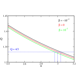
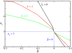
Figure 1: Left panel: representation of the function $\mathcal{Q}=\mathcal{Q}(n)$ [see Eq.(3)], for $N=2$, $L=0$, $\beta=-10^{-3}$ (black line), 0 (red line) and $10^{-3}$ (green line). The plot shows that an unstable configuration in the isotropic limit can become stable if $\beta<0$. Vice versa, when $\beta>0$, a stable configuration in the isotropic limit can become unstable. Right panel: Critical value of the polytropic exponent $n_{c}$ as a function of the anisotropy parameter $\beta$, for $L=0$, 1 and 2.

3 Applications

3.1 Polytropes

Let us apply Eq.(3) to the study of the stability of the polytropic models advanced by Herrera & Barreto [3]. Leaving out the details of the calculations[2], the anisotropic Lane-Emden equation writes

$$\frac{1}{\xi^{2}}\frac{d}{d\xi}\Big{(}\xi^{2}\frac{d\theta}{d\xi}\Big{)}=-\theta^{n}\mathcal{F}(\beta)\,,$$ (4)

where n is the polytropic exponent, $\beta$ the (dimensionless) anisotropy parameter and $\mathcal{F}(\beta)$ is given by

$$\mathcal{F}(\beta)=1-\frac{\beta}{\xi^{2}\theta^{n}}\frac{d}{d\xi}\Big{[}f(\xi)\xi^{N+1}\Big{]}\,.$$ (5)

In the foregoing expression, the exponent N and the function f depend on the model. In the following, we consider $f(\xi)=(1+\xi)^{L}$ (with $L\in\mathbb{R}$). The isotropic Lane-Emden equation is recovered for $\beta=0$ (implying $\mathcal{F}=1$).

In Fig. 1 (left panel) we have represented the $\mathcal{Q}$-factor [see Eq.(3)] as a function of the polytropic exponent n. The diagram shows dissimilar behaviors according to the sign of the anisotropy parameter.

If $\beta<0$, which corresponds to the radial anisotropy (i.e. $P_{t}<P_{r}$, see Ref.[2]), we observe a tendency towards the stability because the critical value $n_{c}$ of the polytropic exponent for the onset of the instability is larger than $n=3$. On the other hand, for $\beta>0$, which corresponds to the tangential anisotropy (i.e. $P_{t}>P_{r}$), we observe that the rising of the dynamical instability is favored (from the plot, we note that $n_{c}<3$).

In the right panel of Fig. 1 we have represented $n_{c}$ as a function of $\beta$, for three values of the exponent L. The plot shows that $n_{c}>3$ for $\beta<0$, in confirmation of the fact that the (presence of) radial anisotropy leads the system to the stability. If $\beta>0$, by contrast, we find $n_{c}<3$, in confirmation of the fact that the tangential anisotropy favors the rising of the instability.

3.2 Anisotropic stars

In this section we consider two models, advanced by Dev & Gleiser[5], conceived as deviations from the homogeneous model (i.e. $\rho=\rho_{0}$). In formulae

$$P_{t}=P_{r}+C\rho r^{2}\,,$$ (6a)

$$P_{t}=P_{r}(1+C\rho r^{2})\,.$$ (6b)

In the foregoing expressions, C estimates the strength of the anisotropy and can be both positive and negative, a priori. Similarly to the case of polytropes, $C>0$ corresponds to the tangential anisotropy and $C<0$ to the radial anisotropy. Integrating the equilibrium equations by using Eqs.(6a) and (6b), we obtain[5]

$$P_{r}=\rho_{0}^{2}\Big{(}\frac{2\pi G}{3}-C\Big{)}(R^{2}-r^{2})\,,$$ (7a)

$$P_{r}=\frac{2\pi G\rho_{0}}{3C}\Big{[}1-e^{C\rho_{0}(r^{2}-R^{2})}\Big{]}\,.$$ (7b)

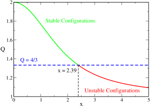
Figure 2: Representation of the function $\mathcal{Q}=\mathcal{Q}(x)$, where x is defined as $x=R\sqrt{C\rho_{0}}$. The plot shows the existence of a critical value $x=\bar{x}$, corresponding to the onset of the dynamical instability. Numerically we find $\bar{x}=2.39$ or, equivalently, $\bar{C}=5.73/(\rho_{0}R^{2})$.

In the previous equations, R and G represent the radius of the star and the gravitational constant, respectively. Concerning the stability, for the ansatz (6a)-(7a), Eq.(3) yields $\mathcal{Q}=2>4/3$, showing that the system is dynamically stable. For the ansatz (6b)-(7b), conversely, we find a more interesting situation. Eq.(3), indeed, takes the form

$$\mathcal{Q}=1+\frac{5}{2x^{2}}-\frac{15}{4x^{4}}+\frac{15D_{+}(x)}{4x^{5}}\geq\frac{4}{3}\,,$$ (8)

where $x=R\sqrt{C\rho_{0}}$ and $D_{+}(x)$ is the Dawson function. In the limit $x\rightarrow 0$, Eq.(8) reduces to $\mathcal{Q}=2>4/3$ that corresponds to the case previously analyzed. On the other hand, for $x\rightarrow+\infty$, we obtain $\mathcal{Q}=1<4/3$ that corresponds to a loss of stability. Consequently, we expect to find a critical value of x allowing the separation between stable and unstable configurations.

In Fig. 2 we have represented Eq.(8) and, as we see, the existence of this critical value is confirmed. Numerically, we find that dynamical instability sets in if $x\geq\bar{x}=2.39$, i.e. if $C\geq\bar{C}=5.73/(\rho_{0}R^{2})$. It is interesting to notice that the stability of the star, rather than the anisotropy parameter, depends on the central density.

3.3 Degenerate fermionic configurations

In this section we focus on the degenerate fermionic configurations, a particular case of a more general study carried out in Ref.[6]. The equation of state (EOS), in a parametric form, is

$$\rho=\frac{4\pi gm^{4}\sigma^{3}}{3h^{3}}\sqrt{W^{3}}\Big{(}1+\frac{2r^{2}}{5r_{a}^{2}}W\Big{)}\,,$$ (9a)

$$P_{r}=\frac{4\pi gm^{4}\sigma^{5}}{15h^{3}}\sqrt{W^{5}}\Big{(}1+\frac{2r^{2}}{7r_{a}^{2}}W\Big{)}\,,$$ (9b)

$$P_{t}=\frac{4\pi gm^{4}\sigma^{5}}{15h^{3}}\sqrt{W^{5}}\Big{(}1+\frac{4r^{2}}{7r_{a}^{2}}W\Big{)}\,.$$ (9c)

In the foregoing expressions, W is the cutoff energy (Fermi energy in this case[6]), $r_{a}$ the anisotropy radius, $\sigma$ the velocity dispersion and the other symbols have their usual meaning. The adiabatic local indexes $\gamma_{r}$ and $\gamma_{t}$ are given by

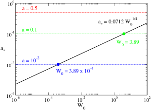
Figure 3: Values of $a_{*}$ as a function of the central density $W_{0}$ [see Eq.(9a)]. The plot shows that, for a given value of a (horizontal lines), there exists a critical value of the central density $W_{0}^{c}$ such that dynamical instabilities set in. For $a=0.5$ (red line) we see that $W_{0}^{c}>>1$ (the system is isotropic and thus stable) whereas, for a $a=0.1$ (green line), we find $W_{0}^{c}=3.89$ and for $a=0.01$ (blue line) we have $W_{0}^{c}=3.89\times 10^{-4}$. This shows that $W_{0}^{c}\rightarrow 0$ for $a\rightarrow 0$ (the system is unstable).

$$\gamma_{r}=\frac{5r_{a}^{2}+2r^{2}W}{7r_{a}^{2}+2r^{2}W}\,\frac{8rW^{2}+7W^{\prime}(5r_{a}^{2}+2r^{2}W)}{8rW^{2}+5W^{\prime}(3r_{a}^{2}+2r^{2}W)}\,,$$ (10a)

$$\gamma_{t}=\frac{5r_{a}^{2}+2r^{2}W}{7r_{a}^{2}+4r^{2}W}\,\frac{16rW^{2}+7W^{\prime}(5r_{a}^{2}+4r^{2}W)}{8rW^{2}+5W^{\prime}(3r_{a}^{2}+2r^{2}W)}\,,$$ (10b)

where $W^{\prime}=dW/dr$. In the isotropic limit $r_{a}\rightarrow+\infty$ the foregoing expressions yield $\gamma_{t}=\gamma_{r}=5/3$. Consequently, according to Eq.(3), we get $\mathcal{Q}=5/3>4/3$ confirming that, in the isotropic limit, degenerate fermionic configurations are stable. Things change in the fully anisotropic regime $r_{a}\rightarrow 0$: we have indeed

$$\gamma_{t}=\gamma_{r}=\frac{4+7y}{4+5y}\,,\quad\mbox{ where }\qquad y=\frac{d\log(W)}{d\log(r)}\,.$$ (11)

As the reader can see, if $-4/5<y<-4/7$, $\gamma_{r}$ and $\gamma_{t}$ are negative. In these conditions, the speed of the two sound waves along the radial and the tangential axis, given by

$$c_{sr}=\sqrt{\frac{\gamma_{r}P_{r}}{\rho}}\,,\quad c_{st}=\sqrt{\frac{\gamma_{t}P_{t}}{\rho}}\,.$$ (12)

become a complex number: the configuration, therefore, is unstable. This feature is a consequence of the trend of density and pressure profiles, which have become “hollow”[6].

Hollow configurations are characterized by the presence of a maximum achieved far from the center. Consequently, the profile is monotonic increasing until the maximum and monotonic decreasing from the maximum until the boundary.

A profile is hollow (and thus unstable) if, for a given value of $W_{0}$, the value of the anisotropy radius $r_{a}$ is below a critical one. To get this critical value, we compute $d^{2}\rho/dr^{2}=0$ at the center and solve for a. Defining the anisotropy parameter as $a=r_{a}/r_{0}$ ($r_{0}$ is a scaling length[6]) and indicating by $a_{*}$ the critical value, we have

$$a_{*}=\frac{r_{a}}{r_{0}}\Big{|}_{critical}=\frac{\sqrt[4]{W_{0}}}{2\pi\sqrt{5}}\,.$$ (13)

In Fig. 3 we have represented the function $a_{*}=a_{*}(W_{0})$. According to the plot, degenerate fermionic configurations are stable if, for a given value of $W_{0}$, $a>a_{*}$ and unstable if $a\leq a_{*}$.

4 Concluding remarks

In this work we have studied the dynamical stability of anisotropic self-gravitating systems. The analysis carried out has shown that, according to the type of anisotropy, the onset of the instability is modified.

In prevalence of radial anisotropy ($P_{r}>P_{t}$), we have observed that the systems have the tendency to evolve towards stable configurations. Unstable configurations in the isotropic limit ($P_{r}=P_{t}$) can become stable. In prevalence of tangential anisotropy ($P_{r}<P_{t}$), by contrast, we have observed that the rising of the instability is favored. Stable configurations in the isotropic limit can become unstable.

In Ref.[2] we have studied the stability of other systems, such as Elliptical Galaxies.

We think that the stability criterion introduced and applied in this work represents a powerful tool for the study of the dynamical stability of a large class of astrophysical systems. The extension of the criterion to General Relativity and other applications will be adressed to forthcoming publications.

References

[1] G. Alberti & M. Merafina, “Proceedings of the Fourteenth Marcel Grossmann Meeting”, 2485 - 2491 (2017)
[2] G. Alberti & M. Merafina, in preparation (2019)
[3] L. Herrera & W. Barreto, Phys. Rev. D 87, 087303 (2013)
[4] F. Shojai, M.R. Fazel, A. Stepanian & M. Kohandel, Eur. Phys. J. C 75, 250 (2015)
[5] K. Dev & M. Gleiser, Gen. Rel. Grav. 35, 1435 (2003)
[6] M. Merafina & G. Alberti, Phys. Rev. D 89, 123010 (2014)