Collisional dynamics of multiple dark solitons in a toroidal Bose-Einstein condensate: Quasiparticle picture

Abstract

We study the collisional dynamics of multiple dark solitons in a Bose-Einstein condensate confined by a toroidal trap. We assume a tight enough confinement in the radial direction to prevent possible dissipative effects due to the presence of solitonic vortices. Analytical expressions for the initial order parameters with imprinted phases are utilized to generate different initial arrays of solitons, for which the time-dependent Gross-Pitaevskii equation is numerically solved. Given that the soliton velocity is conserved due to the lack of dissipation, we are able to apply a simple quasiparticle description of the soliton dynamics. In fact, the trajectory equations are written in terms of the velocities and the angular shifts produced at each collision, in analogy to the infinite one-dimensional system. To calculate the angular shifts, we directly extract them from the trajectories given by the Gross-Pitaevskii simulations and, on the other hand, we show that accurate values can be analytically obtained by adapting a formula valid for the infinite one-dimensional system that involves the healing length, which in our inhomogeneous system must be evaluated in terms of the sound velocity along the azimuthal direction. We further show that very good estimates of such a sound velocity can be directly determined by using the ground state density profile and the values of the imprinted phases. We discuss the possible implementation of the system here proposed using the current experimental techniques.

1 Introduction

Solitons arise as fundamental solutions of nonlinear wave equations ruling in quite diverse systems such as, shallow liquid waves Denardo et al. (1990), magnetic films Chen et al. (1993), complex plasmas Heidemann et al. (2009), and optical fibers Kivshar and Luther-Davies (1998). Particularly, in Bose-Einstein condensates (BECs) solitons are characterized by their form stability under time evolution, even after interacting with other solitons, behaving akin to classical particles. According to the nature of the interatomic interaction occurring in such ultracold gases, that is, an attractive or repulsive one, we may respectively have bright or dark solitons, of which the latter will be in the focus of the present work.

Soliton collisions have been extensively studied in infinite one-dimensional (1D) systems from the theoretical viewpoint Tsuzuki (1971); Zakharov and Shabat (1973); Pitaevskii and Stringari (2003); Konotop (2008); Theocharis et al. (2010). In such systems, solitons collide elastically and continue moving with a constant velocity away from the collision region. Hence, the dynamics of a number of interacting solitons can be described by considering them as quasiparticles moving with constant velocities, whereas the corresponding collisions are regarded as instantaneous shifts in the soliton positions. In a pioneering work, Tsuzuki arrived at a simple relationship between the shifts produced at a collision of two solitary waves Tsuzuki (1971) and later, in Ref. Zakharov and Shabat (1973), an explicit expression for the values of such shifts was obtained. In this formalism each soliton is identified by the corresponding velocity. In a more recent work, it has been shown that very slow solitons, which are identified by their density notches, can be safely regarded as a hard-sphere-like system of particles, which interact through an effective (velocity dependent) repulsive potential Theocharis et al. (2010).

As strictly 1D condensates are impossible to implement experimentally, more realistic soliton systems in atomic BECs confined by different trapping potential geometries have been extensively studied in the last years Frantzeskakis (2010). Recently, renewed interest has arisen from the experimental observation of solitonic vortices in bosonic and fermionic systems Donadello et al. (2014); Ku et al. (2014); Chevy (2014). In such BEC experiments, solitons have been spontaneously created through the Kibble-Zurek mechanism Lamporesi et al. (2013). The so far commonly used candidate to experimentally realize a realistic configuration close to that of the infinite 1D system has been a cigar-shaped condensate. Such a condensate, however, presents the potential drawback of showing a quite different (oscillating) single soliton dynamics. It has been shown that in the Thomas-Fermi approximation a soliton oscillates in a cigar-shaped condensate with the frequency $\omega_{trap}/\sqrt{2}$ Theocharis et al. (2010); Fedichev et al. (1999); Busch and Anglin (2000); Konotop and Pitaevskii (2004); Becker et al. (2008); Wadkin-Snaith and Gangardt (2012), where $\omega_{trap}$ is the angular frequency of the trap in the longitudinal direction. One could avoid, however, such a potentially undesirable effect stemming from the harmonic trap, simply by changing to a toroidal condensate Jezek et al. (2016); Gallucci and Proukakis (2016) .

Experimental setups of toroidal condensates have been extensively utilized for different purposes Ryu et al. (2013); Jendrzejewski et al. (2014); Ryu et al. (2007), particularly, they are currently employed as a fundamental component of test-bed configurations within the emerging field of atomtronics Seaman et al. (2007); Ryu et al. (2013); Jendrzejewski et al. (2014); Eckel et al. (2014). On the other hand, the experimental realization of solitonic initial profiles in such type of condensates could in principle be implemented by standard phase imprinting and/or density manipulation methods, similarly to those applied in cigar-shaped condensates Becker et al. (2008). Actually, an improved phase imprinting protocol for preparing states of given circulation in a toroidal condensate has been recently proposed Kumar et al. (2018). In such work, the authors stated that it would be very interesting to extend these ideas to create multiple solitons with well defined relative velocities. In a recent work Jezek et al. (2016), we have derived an expression for the soliton energy in a toroidal configuration, which depends on the imprinted phases. In particular, we have shown that such an energy turns out to be a decreasing function of the soliton velocity. In such a work, we have studied the dynamics of a pair of symmetrically counter-rotating solitons in a toroidal condensate for a wide range of initial velocities. We note that the soliton velocity $v$ lies between $0$ and $c$ ($0<v<c$), where $c$ is the sound velocity. It has been shown that only for very slow solitons ($v\simeq 0.001c$), the angular velocity remains constant along the evolution except, of course, around the collisions. For larger velocity values, the solitonic profiles are converted in solitonic vortices. In such a work, we were interested in describing the active role that the vortices play in the dynamics. As a consequence of the appearance of solitonic vortices, a continuous increase of the soliton velocities along the evolution was observed, which in turn yields a decrease of the soliton energy that can be interpreted as a dissipative dynamics of the solitonic system. Several other regimes arise from a modulation of the trap parameters Gallucci and Proukakis (2016).

The goal of this work is to study the non dissipative dynamics of gray solitons in a toroidal BEC using a simple quasiparticle picture. We will show that the trajectories, described in terms of the soliton velocities and the angular shifts, can be determined by solely using the density maximum of a Gaussian ground state profile and the imprinted phases. For that purpose, we will model a toroidal condensate tightly enough confined in the radial direction, in order to discard sources of dissipation associated to the presence of solitonic vortices, which may affect the conservation of the soliton velocities. For such trapping parameters, we have found that energy dissipation occurs as the soliton velocity increases during the time evolution. In the present work we will analyze the soliton trajectories arising from time-dependent Gross-Pitaevskii (GP) simulations. In particular, we will demonstrate that the soliton velocities remain constant along the evolution and we will calculate the angular shifts at the collisions. We will show that such shifts can be accurately calculated by only precisely determining the sound velocity for each set of imprinted phases.

It is important to notice that the soliton velocity determines the size of the condensate density notch and hence the “negative” mass of the soliton. Thus, the quasiparticle picture involves solitons with a definite mass. We will show that a rich variety of initial configurations may be reached by implementing certain phase-imprinting protocol.

This paper is organized as follows. In Sec. 2 we introduce the system, particularly the toroidal trap and the set of parameters involved, which are chosen in order to avoid sources of dissipation. In Sec. 3, based on a previous work Jezek et al. (2016), we propose a form of constructing initial arrays of gray solitons with different imprinted velocities. Section 4 is devoted to the study of the soliton dynamics. We first obtain the soliton trajectories along the torus by solving the time-dependent GP equation, showing that in fact, the velocities are conserved, and hence, a simple quasiparticle picture for describing the dynamics can be applied. Within such a picture the quasiparticle collisions are described as angular shifts. A relationship between the angular shifts involved in a collision, analogous to that of the 1D system, is established and, on the other hand, such shifts are evaluated using the trajectories obtained from GP simulations. We also show that very accurate shift values can be analytically obtained by using a few parameters, namely the maximum of the ground state density and the imprinted phases. In addition, we show that the velocity of sound propagating along the angular direction acquires a relevant role in determining the accuracy of the model, and thus we analyze the dependence of such velocity on the imprinted phases. Finally, the conclusions of our study are gathered in Sec. 5.

2 Theoretical framework

We assume a toroidal trapping potential written as the sum of a term depending only on $x$ and $y$, and a term that is harmonic in the $z$ direction:

$$V_{\rm{Trap}}(x,y,z)=V(r)+\frac{1}{2}m\Omega_{z}^{2}z^{2}\,,$$ (1)

where $r^{2}=x^{2}+y^{2}$ and $m$ denotes the atomic mass of ⁸⁷Rb.

The term depending on $r$ is modeled as the following ring-Gaussian potential Murray et al. (2013)

$$V(r)=V_{0}\,\left[1-\exp\left[-\Lambda\left(\frac{r}{r_{0}}-1\right)^{2}\right]\right],$$ (2)

where $V_{0}$ and $r_{0}$ denote the depth and radius of the potential minimum. The dimensionless parameter $\Lambda$ is associated to the $1/e^{2}$ potential width $w=r_{0}\sqrt{\frac{2}{\Lambda}}$.

The trap parameters have been selected to reproduce similar experimental conditions to those described in Ref. Ryu et al. (2013). We have set $V_{0}$=70 nK, $r_{0}$=4 $\mu\rm{m}$, and fixed the particle number to $N=1000$. A high value of $\Omega_{z}=2\pi\times 922$ Hz yields a quasi two-dimensional (2D) condensate which allows a simplified numerical treatment Castin and Dum (1999). Then, the order parameter can be represented as a product of a wave function on the $x$-$y$ plane, $\psi(x,y)$, and a Gaussian wave function along the $z$ coordinate, from which the following 2D interacting parameter can be extracted Castin and Dum (1999)

$$g=g_{3D}\left(\frac{m\Omega_{z}}{2\pi\hbar}\right)^{1/2},$$ (3)

where $g_{3D}=4\pi\hbar^{2}a/m$, being $a=98.98\,a_{0}$ the $s$-wave scattering length of ⁸⁷Rb and $a_{0}$ being the Bohr radius.

In the mean-field approximation, the condensate dynamics is ruled by the time-dependent GP equation

$$i\hbar\frac{\partial\psi}{\partial t}=\left[-\frac{\hbar^{2}}{2m}{\bf\nabla}^{2}+V(r)+g\,|\psi|^{2}\right]\psi,$$ (4)

where $\psi\equiv\psi(x,y,t)$ denotes a 2D order parameter normalized to the number of particles. Finally, as will be discussed in the next section, a high value of the dimensionless parameter $\Lambda=50$ ($w=0.8$ $\mu\rm{m}$) is assumed, in order to assure a condensate confinement in the radial direction that avoids the appearance of solitonic vortices in the dynamics.

3 Initial arrays of gray solitons

In a previous work Jezek et al. (2016), we have shown that for a similar toroidal trap, a dark soliton located along the $x$-axis may be safely modeled through an order parameter with a Gaussian profile of the form,

$$\psi_{G}(r,\theta) = \sqrt{n(X)}\,\exp\left[-\frac{\gamma}{2}\left(1-\frac{r}{r_{0}}\right)^{2}\right]$$

$$\times \left[\sqrt{1-X^{2}}\tanh\left(\sqrt{1-X^{2}}\,{\rm k}r\sin\theta\right)+iX\right],$$

with ${\rm k}=\sqrt{n(X=0)gm}/\hbar$ and $n(X)=n_{0}/(1-\frac{2\sqrt{1-X^{2}}}{\pi{\rm k}r_{0}})$, where $0\leq X\leq 1$, and $n_{0}$ denotes the ground-state density maximum located at $r=r_{0}$. For $X=1$ one recovers the ground state, whereas for $X=0$ a stationary state with a double-notch with vanishing density is obtained, which is referred to as a black soliton. Gray solitons are determined by the intermediate values $0<X<1$, which define the absolute value of the soliton initial velocity in units of the sound speed. Such gray solitons are characterized by having non vanishing density notches. It is important to note that the subsequent dynamics of the gray soliton initial order parameter actually corresponds to a pair of symmetrically counter-rotating solitons, with the soliton initially located across the torus at $x<0$ ($x>0$) moving clockwise (counterclockwise) Jezek et al. (2016). As the number of particles is fixed, $n(X)$ is a decreasing function of $X$, which is due to the fact that for a smaller $X$ more particles are expelled from the density notch. It is easy to propose a generalization of the above ansatz for an initial state consisting of an even number $N_{S}$ of rotating solitons:

$$\psi_{G}(r,\theta) =A\,\exp\left[-\frac{\gamma}{2}\left(1-\frac{r}{r_{0}}\right)^{2}\right]$$ (6)

$$\prod_{j=1}^{N_{S}/2}\left[\sqrt{1-X_{j}^{2}}\tanh\left(\sqrt{1-X_{j}^{2}}\,{\rm k}r\sin(\theta-\alpha_{j})\right)\right.$$

$$+iX_{j}\left.\right],$$

being $A$ a normalization constant and ${\rm k}=\frac{\sqrt{n_{0}gm}}{\hbar}$. Here the pair of gray solitons labeled by the subscript $j$ are assumed to be initially located along an axis forming an angle $\alpha_{j}$ with the $x$-axis, and they move counter-rotationally at an angular speed determined by the parameter $X_{j}$ ($0<X_{j}<1$). We note that the phase between adjacent density notches turns out to be a flat function of $\theta$, i.e., it does not present any gradient around the torus, which would be the case if single-notch solitons were generated for each parameter $X_{j}$ Kumar et al. (2018).

In Fig. 1, we depict the densities corresponding to the stationary solutions of the GP equation for the ground state ($X_{j}=1$) and the four-notch black soliton ($X_{j}=0$), which are very similar to those predicted by the Gaussian model (6) with ${\rm k}=1.95\,\mu$m^-1. It is worthwhile noticing that the density maximum of the four-notch black soliton configuration turns out to be appreciably higher than that of the ground state, because a large number of atoms are expelled from the density notches. Fig. 2 shows the GP order parameter of the four-notch black soliton as a function of the angular coordinate for $r=r_{0}$, which shows a very good agreement with that given by the Gaussian model, as well. Such a profile also quantitatively agrees with the kinks observed in the second-excited stationary analytic solution of a strictly 1D ring ruled by the nonlinear Schrödinger equation Carr et al. (2000), and the same agreement was observed between the double-notch black soliton and the two-node first-excited solution of the 1D ring system Jezek et al. (2016).

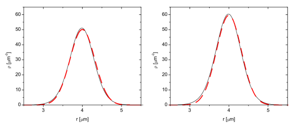
Figure 1: Density profiles $\rho(r,\theta)=|\psi(r,\theta)|^{2}$ as functions of the radial coordinate $r$ for the ground state (left panel), and the four-notch black soliton (right panel) calculated at $\theta=\pi/4$. Black solid lines correspond to the GP density, whereas the red dashed lines correspond to the Gaussian model (6) for $X_{j}=1$ (left panel) and $X_{j}=0$ (right panel) with $\alpha_{1}=0$ and $\alpha_{2}=\pi/2$.

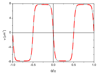
Figure 2: The four-notch black soliton order parameter as a function of the angular coordinate calculated at the potential minimum $r=r_{0}=4\,\mu$m. The black solid line corresponds to the GP solution, whereas the red dashed line corresponds to the Gaussian model (6) for $X_{j}=0$ with $\alpha_{1}=0$ and $\alpha_{2}=\pi/2$.

The value of $\gamma$ in Eq. (6) has been determined by minimizing the energy per particle,

$$E(\gamma) = \frac{1}{N}\int d^{2}{\bf r}\,\,\psi_{G}(r,\theta,\gamma)\left[-\frac{\hbar^{2}}{2m}{\bf\nabla}^{2}+V(r)\right.$$ (7)

$$+ \left.\frac{g}{2}\,|\psi_{G}(r,\theta,\gamma)|^{2}\right]\psi_{G}(r,\theta,\gamma),$$

where $\psi_{G}(r,\theta,\gamma)$ is the order parameter given by Eq. (6) with $X_{j}=1$ and $\gamma$ is used as a variational parameter. We depict in Fig. 3 such an energy as a function of $\gamma$, whose minimum turns out to be around 80. On the other hand, we have found the following analytical approximation valid for $\gamma>>1$,

$$E(\gamma)=\frac{\hbar^{2}}{4Mr_{0}^{2}}\,\gamma+V_{0}\left[1-\sqrt{\frac{\gamma}{\Lambda+\gamma}}\right]+\frac{Ng}{2^{\frac{5}{2}}\pi^{3/2}r_{0}^{2}}\,\gamma^{1/2},$$ (8)

where the first, second and third term on the right-hand side, correspond to the kinetic, trap and interaction energies, respectively. Such an expression shows an excellent agreement with the numerically integrated energy, as seen in Fig. 3. We have found that the error in using such an expression turns out to be less than 0.01 % for $\gamma>30$. Therefore, the value of $\gamma$ for the energy minimum can be safely obtained by using Eq. (8) for our parameter range, which in fact yields $\gamma=80$.

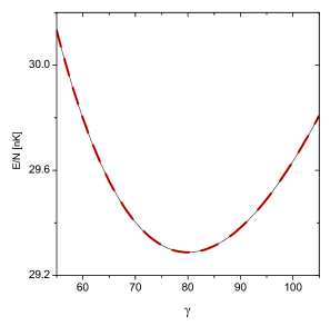
Figure 3: Energy per particle corresponding to the soliton-free order parameter (6) as a function of the Gaussian parameter $\gamma$. The red dashed line corresponds to the analytic expression given by Eq. (8), whereas the black solid line corresponds to a numerical integration of the energy.

The values of the trap parameter $\Lambda$ and the number of particles have been selected according to a recent work by Gallucci and Proukakis Gallucci and Proukakis (2016), where the authors studied the regimes that appear in the dynamics when varying the dimensionless parameter $l_{r}/\zeta_{0}$ for a similar trapping potential, where $l_{r}=\sqrt{\hbar/m\omega_{r}}$ corresponds to the harmonic oscillator length and $\zeta_{0}=\frac{\hbar}{\sqrt{n_{0}gm}}$ denotes the healing length. Three distinct regimes were identified: solitonic (stable), shedding, and snaking (unstable). In particular, the solitonic regime features an internal subdivision around $l_{r}/\zeta_{0}=1$ Gallucci and Proukakis (2016). Here we want to avoid the appearance of solitonic vortices and thus we restrict ourselves to the regime defined by $l_{r}/\zeta_{0}<1$, where radial excitations are suppressed. We have found that with a high $\Lambda=50$ and a number of particles $N=1000$ such a relation is verified. More precisely, the size of the condensate in the radial direction may be directly estimated from the expression of the Gaussian density compared to that of a harmonic oscillator trapping potential:

$$\psi^{2}_{G}(r)=A\,\exp\left[-\gamma\left(1-\frac{r}{r_{0}}\right)^{2}\right]\,=A\,\exp\left[-\frac{\left(r-r_{0}\right)^{2}}{l_{r}^{2}}\right]$$ (9)

leading to $l_{r}=r_{0}/\sqrt{\gamma}=0.447$ $\mu$m. On the other hand, we have $\zeta_{0}=0.51$ $\mu$m for the healing length, which confirms us that we are within the pursued regime. Here it is worthwhile noticing that in our previous work Jezek et al. (2016), these quantities yielded $l_{r}=0.685$ $\mu$m and $\zeta_{0}=0.50$ $\mu$m, consistent with the fact that we were also interested in exploring how the presence of vortices affects the dynamics. In fact, in such a work it was shown that the solitons become accelerated, a signature of dissipative effects that appear when solitonic vortices are formed.

4 The dynamics

4.1 GP numerical simulations

To analyze the soliton dynamics, we have numerically solved the time-dependent GP equation for initial order parameters of the form (6) with different soliton velocities. For all cases we have used $\alpha_{1}=0$ and $\alpha_{2}=-\pi/2$, in order to obtain four well separated initial soliton dips. In Fig. 4, we show snapshots of the density and phase for the case $X_{1}=0.2$ and $X_{2}=0.4$, where the top panels correspond to the initial configuration and the bottom panels illustrate how the phase remains almost constant at both sides of each density dip during the evolution, aside from small fluctuations associated to sound excitations. In particular, it may be seen at the bottom panels that the slower solitons, which exhibit the deeper density notches, have performed half a cycle around the torus, while the faster solitons have almost completed an entire one. We note that such a time turns out to be about 14% smaller than the one corresponding to the same trajectory of noninteracting solitons.

It is worthwhile noticing that initial states of this kind can be experimentally achieved by using a phase imprinting method consisting in illuminating the bottom ($y<0$) and left ($x<0$) half-spaces with different intensities, where, in the case of the top panel of Fig. 4, the former intensity has been assumed to be higher than the latter. The impression of such a distribution of phases can be experimentally implemented by using a Spatial Light Modulator (SLM) Kumar et al. (2018) with different intensities in each quadrant of the $(x,y)$-plane that fulfill the above mentioned condition.

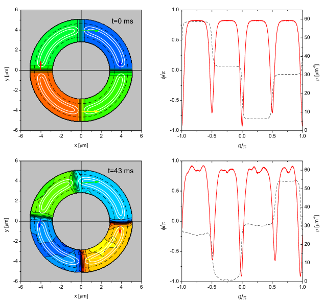
Figure 4: In the left panels we show the phase distribution (colors) and particle density isocontours (white solid lines) for a GP time dependent simulation with an initial condition obtained from Eq. (6) for $X_{1}=0.2$ and $X_{2}=0.4$. The top and bottom panels correspond to snapshots taken at $t=0$ and $t=43$ ms, respectively. A dashed line is also shown at the left panels to denote isocontours corresponding to a 10 percent of the maximum density of the ground state, while the arrows indicate the soliton velocities and their colors identify each soliton. The right panels show angular distributions of the particle density (red solid line) and phase (black dashed line) for the azimuthal angle $\theta$ at the radius $r_{0}=4\,\mu$m. The phase colors at the left panels are linked to the corresponding phase values depicted on the right panels.

The numerical evolutions for three initial arrays are depicted in Fig. 5, where we show the ($k$)-soliton angular position $\theta_{k}(t)$ (left panels) and the corresponding phase difference $\Delta\phi_{k}$ between both sides of the ($k$)-soliton (right panels). We are assigning the prefix value $k=j(-j)$ to the soliton with positive (negative) angular velocity imprinted through the parameter $X_{j}$. In such arrays, the combination of values of the parameters $X_{j}$ have been chosen to cover the distinct behaviors at collisions. It is important to observe that in all cases, each soliton moves with a constant angular velocity, except near collisions, as may be seen in the left panels of Fig. 5. Hence, the quasiparticle picture for describing the dynamics of our soliton system turns out to be plausible. We note that the mass associated with a soliton depends on the depth of the soliton density notch, which in turn depends on its velocity. Then, we may say that each soliton behaves as a quasiparticle with a fixed mass. In contrast to the configuration studied in Ref. Jezek et al. (2016), all the present cases have shown that solitons can undergo many collisions without evidencing any signature of energy dissipation that could be inferred from a velocity increase.

It is worthwhile mentioning that in an experimental work on bright solitons Nguyen et al. (2014), it has been shown that in an asymmetric collision, the solitons pass through one another and emerge from the collision unaltered in shape, amplitude, or velocity, but with a new trajectory. It is important to remark that this behavior is also observed for dark solitons in all the simulations we have performed, as can be seen in Fig. 5. In contrast, such an effect cannot be discerned in the simulations of Ref. Jezek et al. (2016), where only symmetric collisions take place and hence each soliton cannot be distinguished.

We notice that during an asymmetric collision the precise location of the faster soliton could eventually become undetermined, if its density minimum disappears at merging with the deeper density minimum of the slower soliton, when the distance between both density dips becomes smaller than two healing lengths. This is the case for the faster solitons of the middle and bottom left panels of Fig. 5.

The imprinted phase difference can be estimated by considering the asymptotic values $\pm 1$ of the hyperbolic tangent in Eq. (6), which determine the phase at each side of the soliton density notch as the phases of the complex numbers $\pm\sqrt{1-X_{j}^{2}}+iX_{j}$, yielding the initial phase difference

$$\Delta\phi_{\pm j}=\mp\,2\cos^{-1}(X_{j})$$ (10)

for the ($\pm j$)-soliton. It is worthwhile noticing that the above expression can be used in an experiment to obtain the parameters $X_{j}$ by using the values of the imprinted local phases.

In the right panels of Fig. 5, we show the initial values obtained from Eq. (10) as horizontal dashed lines. Note that the mean value of each phase difference remains around its initial value, except near collisions. Such a behavior is also a signature of the lack of dissipation in the soliton system, as the phase difference is directly linked to the soliton velocity through Eq. (10). In particular, from the time evolutions provided by the simulations in Ref. Jezek et al. (2016), it may be seen that whenever the main absolute value of the phase difference decreases, the absolute value of the velocity increases.

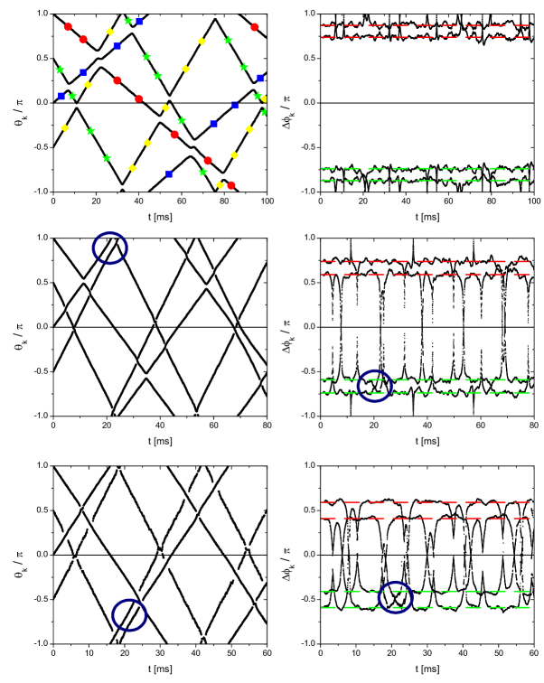
Figure 5: Time evolutions of the soliton angular positions (left panels) and phase differences at both sides of each density minimum (right panels), for the initial order parameter (6) with $\alpha_{1}=0$, $\alpha_{2}=-\pi/2$, and $X_{1}=0.2$ and $X_{2}=0.4$ ( top panel ), $X_{1}=0.4$ and $X_{2}=0.6$ (middle panel), and $X_{1}=0.6$ and $X_{2}=0.8$ (bottom panel). The horizontal red (green) dashed lines on the right panels indicate the initial phase difference given by Eq. (10) for the $j(-j)$-soliton. The empty blue circles in the middle and bottom panels locate the overtaking collisions mentioned in the text. Circles, squares, stars, and diamonds are depicted at the top left panel to guide the eye on the different quasiparticle trajectories. The symbols have the same color of the arrows that distinguish each soliton at the left panels of Fig. 4.

Taking into account the head-on collisions, we can distinguish the following characteristics. In the top right panel of Fig. 5, we may observe that the phase differences at collisions reach $\pm\pi$ for $X_{1}=0.2$ and $X_{2}=0.4$, which is in accordance with that observed in Ref. Jezek et al. (2016) for velocities slower than half the sound speed ( $X_{j}<0.5$). On the other hand, for $X_{1}=0.6$ and $X_{2}=0.8$ (bottom panel), we have both soliton velocities above such a limit and the phase differences vanish at collisions, remaining bounded along the whole evolution, as previously observed for symmetric collisions Jezek et al. (2016). Finally, we may observe in the middle right panel that both behaviors coexist for $X_{1}=0.4$ and $X_{2}=0.6$, as expected.

A different class of soliton interaction, arising only for asymmetric collisions, takes place when an overtaking event occurs. Such overtaking collisions can be viewed for example in the middle and bottom panels of Fig. 5, indicated by the empty circles at $t\simeq 20$ ms and $t\simeq 22$ ms, respectively. Note also in the right panels, the phase difference approaches that can be observed in between adjacent horizontal dashed lines for this kind of collisions, in contrast to the above high velocity head-on collisions, where the phase differences go to zero.

4.2 Quasiparticle picture

In this subsection we will treat the solitons as quasiparticles. In this picture, each quasiparticle has a fixed (negative) mass and can freely move in the angular direction. The interaction between such quasiparticles occurs through a particular type of collision, where both colliding quasiparticles are transmitted through each other without altering their velocity. As a consequence of such a collision, an angular shift on each soliton position is produced. We recall that this behavior has been experimentally observed for bright solitons Nguyen et al. (2014).

By means of the GP numerical simulations, we have shown that the velocity of each soliton remains constant, except around collisions. As a consequence, the depth of the soliton density dip is conserved, which implies that the soliton mass is also conserved. Hence, the quasiparticle description can be safely applied and the trajectory $\theta_{k}(t)$ of a soliton with angular velocity $\omega_{k}$ can be written as,

$$\theta_{k}(t)=\omega_{k}t+\sum_{l}\Delta\theta_{k}(t_{l})\,\,{\cal U}(t-t_{l})+\theta_{k}(0),$$ (11)

where ${\cal U}(t-t_{l})$ denotes the unit step function, $t_{l}$ indicates the time of the $l$-th collision, and $\Delta\theta_{k}(t_{l})$ designates the angular shift produced at such a collision.

We note that the number of collisions, in contrast to the 1D infinite case, is not upper bounded and could take any value, depending on the time interval involved. However, we will see that the shifts could only take a few different values.

As seen in the previous section, we have considered initial configurations with two distinct values of the parameter $X_{j}$, which gives rise to a system of four rotating solitons, each one identified by its corresponding angular velocity $\omega_{k}$. We will see that such a system could yield only six absolute values of the shift. In the next subsections, we will derive a relation between the shifts involved in an asymmetric collision, and we will also evaluate all of them using a numerical method and an analytical approach.

4.2.1 Theoretical treatment of the shifts

In an infinite 1D system, the spatial shifts $\Delta z_{i}$ at a collision have been analytically obtained using the explicit form of the order parameter Zakharov and Shabat (1973) as,

$$|\Delta z_{i}| = \frac{\zeta}{2\sqrt{1-Y_{i}^{2}}}$$ (12)

$$\times \ln\left[\frac{\left(Y_{i}-Y_{j}\right)^{2}+\left(\sqrt{1-Y_{i}^{2}}+\sqrt{1-Y_{j}^{2}}\right)^{2}}{\left(Y_{i}-Y_{j}\right)^{2}+\left(\sqrt{1-Y_{i}^{2}}-\sqrt{1-Y_{j}^{2}}\right)^{2}}\right],$$

where $i=1,2$ and $j=1,2$, with $i\neq j$. Here $Y_{k}=\dot{z}_{k}/c$ represents the velocity (in units of the sound speed $c$) of the corresponding soliton and $\zeta$ denotes the healing length of the homogeneous system. Both shifts have always opposite signs and, as previously demonstrated by Tzusuki Tsuzuki (1971) by analyzing the motion of the soliton mass center during a collision, they fulfill the following relation

$$\Delta z_{1}\sqrt{1-Y_{1}^{2}}+\Delta z_{2}\sqrt{1-Y_{2}^{2}}=0.$$ (13)

In our toroidal configuration, the hypothesis of conservation of the linear momentum does not remain valid, however, by applying the conservation of the angular momentum, we will see that an analogous expression to (13) can still hold. We will assume solitons as point-quasiparticles with masses $M_{i}$ that move at a fixed radius $r_{0}$.

Considering a time interval ($0\leq t\leq t_{f}$) where a single collision takes place, which occurs between the $(1)$- and $(2)$-soliton at $t=t_{c}<t_{f}$, and using Eq. (11), we obtain both soliton angular velocities,

$$\dot{\theta}_{1}(t)=\omega_{1}+\Delta\theta_{1,2}\,\,\frac{d}{dt}{\cal U}(t-t_{c}),$$ (14)

$$\dot{\theta_{2}}(t)=\omega_{2}+\Delta\theta_{2,1}\,\,\frac{d}{dt}{\cal U}(t-t_{c}),$$ (15)

where $\Delta\theta_{1,2}=\Delta\theta_{1}(t_{c})$ denotes the angular shift on $\theta_{1}$ produced by the collision with the ($2$)-soliton. Hereafter, all the angular shifts will be identified by the subscripts of the solitons involved in the corresponding collision.

Multiplying the above angular velocities by the square of the radius $r^{2}_{0}$ and the corresponding soliton mass $M_{i}$, we can write the expressions for each soliton angular momentum as,

$$\vec{L}_{1}=M_{1}r^{2}_{0}\,\omega_{1}\hat{z}+\frac{d}{dt}\left[M_{1}r^{2}_{0}\Delta\theta_{1,2}\,\,{\cal U}(t-t_{c})\right]\hat{z},$$ (16)

$$\vec{L}_{2}=M_{2}r^{2}_{0}\,\omega_{2}\hat{z}+\frac{d}{dt}\left[M_{2}r^{2}_{0}\Delta\theta_{2,1}\,\,{\cal U}(t-t_{c})\right]\hat{z},$$ (17)

where $\hat{z}$ denotes the $z$-coordinate unit vector. Now, assuming that the total angular momentum $\vec{L}=\vec{L}_{1}+\vec{L}_{2}$ must be conserved, the sum of the second terms of Eqs. (16) and (17), should at least be bounded. Rearranging such a sum we have,

$$\frac{d}{dt}\left[r^{2}_{0}(M_{1}\Delta\theta_{1,2}\,+M_{2}\Delta\theta_{2,1})\,\,{\cal U}(t-t_{c})\right]$$ (18)

and hence, applying to this quantity the condition of being bounded leads to,

$$M_{1}\Delta\theta_{1,2}+M_{2}\Delta\theta_{2,1}=0.$$ (19)

On the other hand, the negative mass of the soliton Becker et al. (2008); Wadkin-Snaith and Gangardt (2012) can be estimated by using Eq. (6) to calculate the number of particles expelled from the core, yielding

$$M_{i}=-2mA^{2}\frac{\sqrt{1-X_{i}^{2}}}{k}\int dr\frac{r}{r_{0}}\,\exp\left[-\gamma\left(1-\frac{r}{r_{0}}\right)^{2}\right],$$ (20)

which replaced in (19) leads to the following expression analogous to (13),

$$\Delta\theta_{1,2}\sqrt{1-X_{1}^{2}}+\Delta\theta_{2,1}\sqrt{1-X_{2}^{2}}=0$$ (21)

for our toroidal configuration.

Given that our condensate is not a 1D ring, we do not have analytical solutions of our solitonic system, and hence we cannot derive an analogous formula to (12) for the shift values. Nevertheless, in the next section we will show that accurate values can be obtained by adapting (12) in a convenient manner. We want to note that, being our system non homogeneous, the way we adopt for evaluating the healing length becomes crucial to guarantee such an accuracy in the values of the shifts.

4.2.2 Numerical and analytical determination of the angular shifts

In order to numerically determine the angular shifts, we have run a GP simulation for an initial condition with $X_{1}=0.6$ and $X_{2}=0.2$, where, as seen in Fig. 6, it is clearly shown that there exist four different types of collisions. By measuring each slope of the four numerically obtained trajectories $\theta_{k}(t)$ ($k=\pm 1,\pm 2$), we have determined the soliton angular velocities $\omega_{1}=(0.060\pm 0.001)\,\pi\,\rm{ms}^{-1}$ and $\omega_{2}=(0.020\pm 0.001)\,\pi\,\rm{ms}^{-1}$, being $\omega_{-k}=-\omega_{k}$. Here it is important to notice that, in analogy to the infinite 1D case, where $X_{j}=v_{j}/c$, with $v_{j}$ the soliton (linear) speed, we may write $c(X_{1},X_{2})=\omega_{1}r_{0}/X_{1}=\omega_{2}r_{0}/X_{2}$. Thus, we can utilize such a proportionality to extract an estimate of the linear speed of sound azimuthally propagating along our ring-shaped condensate, yielding $c\simeq\,1.26\,\mu$m/ms.

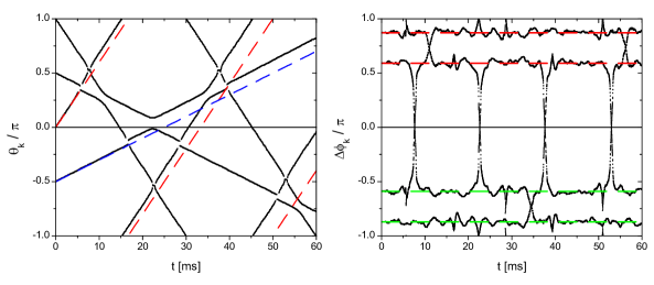
Figure 6: Same as Fig. 5 for $X_{1}=0.6$ and $X_{2}=0.2$. The dashed lines in the left panel indicate noninteracting trajectories for the (1)-soliton (red) and the (2)-soliton (blue).

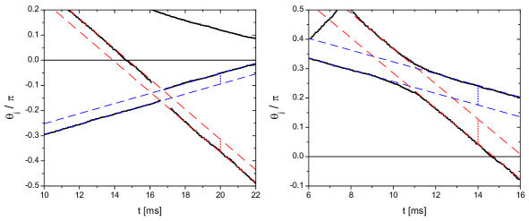
Figure 7: Enlarged graphs of both kinds of asymmetric collisions represented at the left panel of Fig. 6. The left (right) panel shows a head-on (overtaking) collision with dashed lines tangent to the trajectories before and after the collisions, while the vertical dotted lines indicate the corresponding shifts.

To illustrate the way we have calculated the angular shifts, in Fig. 7 we show close-ups of both kinds of asymmetric collisions displayed at the left panel of the previous figure, drawing the tangent lines to the soliton trajectories before and after the collisions, with slopes corresponding to the aforementioned angular velocities. This in turn determines the shifts denoted by the vertical dashed lines. Due to the Cartesian grid, the error in the determination of the angular shifts is about $0.003\pi$. Particularly, for the head-on collision Stellmer et al. (2008); Huang et al. (2001) which involves the ($-1$)- and ($2$)-soliton, depicted in the left panel, we obtained for the angular shift on the $(-1)$-soliton $|\Delta\theta_{-1,2}|=0.051\pi$ and for the angular shift on the $(2)$-soliton $|\Delta\theta_{2,-1}|=0.042\pi$. So, the quotient turns out to be $|\Delta\theta_{2,-1}/\Delta\theta_{-1,2}|=0.82\pm 0.07$, which yields a good agreement with the result
$\sqrt{1-X_{1}^{2}}/\sqrt{1-X_{2}^{2}}=0.81$, in accordance with Eq. (21). We note that a collision between the $(1)$- and the $(-2)$-soliton yields the same preceding absolute values of the angular shifts, i.e, $|\Delta\theta_{1,-2}|=|\Delta\theta_{-1,2}|$ and $|\Delta\theta_{-2,1}|=|\Delta\theta_{2,-1}|$.

On the other hand, for the overtaking collision shown on the right panel of Fig. 7 that involves the ($-1$)- and ($-2$)-soliton, we obtained $|\Delta\theta_{-1,-2}|=0.084\pi$ and
$|\Delta\theta_{-2,-1}|=0.067\pi$, which yields a quotient
$|\Delta\theta_{-2,-1}/\Delta\theta_{-1,-2}|=0.80\pm 0.07$ that again equals
$\sqrt{1-X_{1}^{2}}/\sqrt{1-X_{2}^{2}}$, within the predicted error. Once more, the ($1$)- and ($2$)-soliton would yield the same shift values.

We have calculated in a similar fashion the shifts in the symmetric collisions, which yielded $|\Delta\theta_{1,-1}|=|\Delta\theta_{-1,1}|=0.030\pi$ and $|\Delta\theta_{2,-2}|=|\Delta\theta_{-2,2}|=0.076\pi$.

In summary, for our particular four-soliton system only six different absolute values of the angular shifts are obtained, which are given in Table 1. In particular, we have two symmetric collisions, each one involving a single absolute value of the shift, and two types of asymmetric collisions which give rise to the remaining four absolute values.

In view of the analogy between Eqs. (13) and (21), it becomes evident that one could also try to adapt formula (12) to our present toroidal geometry. Thus, taking into account that the parameters $X_{j}$ are defined as positive quantities, we may obtain the absolute values of the different angular shifts as,

$$|\Delta\theta_{-i,\pm j}|/\pi=\frac{\zeta^{*}/(\pi r_{0})}{2\sqrt{1-X_{i}^{2}}}$$

$$\times\ln\left[\frac{\left(X_{i}\pm X_{j}\right)^{2}+\left(\sqrt{1-X_{i}^{2}}+\sqrt{1-X_{j}^{2}}\right)^{2}}{\left(X_{i}\pm X_{j}\right)^{2}+\left(\sqrt{1-X_{i}^{2}}-\sqrt{1-X_{j}^{2}}\right)^{2}}\right],$$ (22)

where $i=1,2$ and $j=1,2$. The sign $+$ ($-$) corresponds to head-on (overtaking) collisions. Here it is important to recall that, as our system is non homogeneous, the value of the healing length would depend on the density of the selected point at which it is calculated. Conversely, the value of the sound speed, obtained in the previous section, only depends on well defined quantities: $X_{j}$ and the ($j$)-soliton velocity. Hence, we have utilized the expression $\zeta^{*}=\hbar/(mc)$ for calculating the healing length with our above estimate of the sound speed, $c=\,1.26\,\mu$m/ms, which yields $\zeta^{*}=0.575\,\mu$m. The corresponding results arising from Eq. (22), which agree very well with those obtained from numerical simulations, are summarized in Table 1. Also it is worth noting that the use of other common estimates of the healing length, such as that derived for a homogeneous system at the density maximum, would have yielded an underestimated shift in about a 20 percent.

Table 1: Absolute value of the angular shifts (in units of $\pi$) produced at the collisions.

Type of collision	$X_{k}$	Simulation	Eq. (22)
Head-on asymmetric	$0.6$	$0.051$	$0.050$
	$0.2$	$0.042$	$0.041$
Overtaking asymmetric	$0.6$	$0.084$	$0.082$
	$0.2$	$0.067$	$0.067$
Head-on symmetric	$0.6$	$0.030$	$0.029$
	$0.2$	$0.076$	$0.076$

4.2.3 Sound velocity

Given the importance that the sound velocity acquires for determining the angular shifts, we have obtained its numerical values when varying the imprinted phases by using the relationship $c(X_{1},X_{2})=\omega_{j}r_{0}/X_{j}$. Such values are depicted as solid circles in Fig. 8, as a function of the square root of the soliton density maximum. On the other hand, we have theoretically derived an analytic formula for the sound velocity in terms of our soliton 2D density maximum. With such a purpose, we have used the result that the sound propagation speed in an elongated condensate reads $c=\sqrt{g\bar{n}/m}$ Kavoulakis and Pethick (1998), where $\bar{n}$ is the averaged density in the transversal direction. Then, we have considered a 2D elongated condensate with a density profile in the transversal direction defined by the coordinate $r$ that emulates the density profile of our solitonic system far from the density notches, which, using (6) can be modeled as,

$$n(r)=n_{max}\,\exp\left[-\gamma\left(1-\frac{r}{r_{0}}\right)^{2}\right],$$ (23)

where $n_{max}$ denotes the density maximum. Such a maximum changes with the imprinted phases and hence it depends on $X_{1}$ and $X_{2}$. An analytical expression for
$n_{max}(X_{1},X_{2})$ will be derived below. Using the above profile, we have calculated the mean value $\bar{n}=\int n^{2}dr/\int ndr$, which yields $\bar{n}=n_{max}/\sqrt{2}$ and hence $c=\sqrt{gn_{max}/\sqrt{2}m}$. It is worthwhile recalling that in the three-dimensional case, the value $\bar{n}=n_{max}/2$ is obtained Kavoulakis and Pethick (1998). It can be seen in Fig. 8 that the curve $c=\sqrt{gn_{max}/\sqrt{2}m}$ is in a very good accordance with the set of points obtained from the time dependent simulations. On the other hand, the upper curve $c=\sqrt{gn_{max}/m}$ represents the velocity that should be used to calculate the healing length by employing its analytical expression as a function of the local density $\zeta=\hbar/\sqrt{n_{max}gm}$. For completeness we have also depicted the function $c=\sqrt{gn_{max}/2m}$ (lower line), which represents the expression for a three-dimensional density.

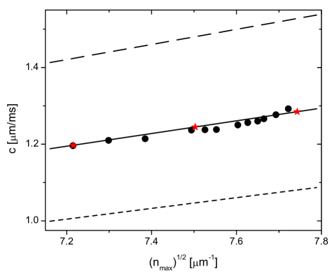
Figure 8: Sound velocity as a function of the square root of the density maximum $n_{max}$. The solid line corresponds to $c=\sqrt{gn_{max}/\sqrt{2}m}$, which has been extracted by using the Gaussian density profile. The dashed (dotted) line corresponds to $c=\sqrt{gn_{max}/m}$ ($c=\sqrt{gn_{max}/2m}$). The black solid circles have been obtained from GP simulations in the manner outlined in Sec. 4.2.2. The red stars correspond to the sound velocity derived in Sec. 4.2.3, with the densities obtained from Eq. (24) for $(X_{1},X_{2})=(0.9,1),(0.7,0.8)$, and $(0.1,0.2)$, from left to right.

As we are dealing with a fixed total number of particles, the value of $n_{max}$ increases with the imprinted phase difference. In particular, $n_{max}(X_{1},X_{2})$ aquires its maximum value when $X_{1}=X_{2}=0$, which corresponds to a black soliton. We can go further and obtain an analytical expression for such a quantity by evaluating the amount of particles expelled from the place where each soliton density notch is formed, instead of using $n_{max}=A^{2}$ of Eq. (6). Thus we obtain,

$$n_{max}(X_{1},X_{2})=\frac{n_{0}}{1-\frac{2\sqrt{1-X_{1}^{2}}}{\pi{\rm k}r_{0}}-\frac{2\sqrt{1-X_{2}^{2}}}{\pi{\rm k}r_{0}}}$$ (24)

where $n_{0}=n_{max}(X_{1}=1,X_{2}=1)$ is the ground state density maximum. We have found that with such an estimate, the sound velocity is obtained within a relative error of $2$ percent. We have plotted as red stars in Fig. 8 some representative points obtained by using this simplified protocol. The nearest black solid circles, obtained from the time dependent simulations, correspond to the same set of parameters $X_{1}$ and $X_{2}$. From these results, we may conclude that a good quasiparticle description can be achieved by solely using the ground state density and the imprinted phases. It is worthwhile noticing that, given that the experimental images correspond to integrated densities along the direction through which the condensate is viewed, yielding thus images proportional to 2D densities, our result could also be applicable to such configurations.

4.2.4 Accumulative shift effect

Here it is important to note that, although each individual shift at a collision may not be expected to lie within the reach of the available experimental resolution Stellmer et al. (2008), an accumulative effect of the shifts during one period could in principle be experimentally detectable. The magnitude of such an effect can be viewed in Fig. 6, where one can observe that the collisions cause a sizable advance on the soliton dynamics, as compared to the trajectories of ideally noninteracting solitons, which are depicted as dashed lines. We can analytically estimate this effect by using the velocities and the angular shifts. For instance, the period for the noninteracting trajectory starting at $\theta=0$ turns out to be 33.3 ms, whereas the shifts produced at each collision bring about that this time becomes effectively reduced. In particular, we may see that the corresponding (1)-soliton undergoes two asymmetric and two symmetric collisions during such a time interval, with an estimated reduction in time $|\Delta\theta_{1,k}/\omega_{1}|$ at each collision with another $(k)$-soliton, which yields a reduction in the whole period of about 2.7 ms ($\sim 10\%$). On the other hand, for the trajectory that starts at $\theta=-\pi/2$ that corresponds to the (2)-soliton, we obtain that its half-period becomes reduced in 4.7 ms with respect to the noninteracting one (50 ms), which means again about a $10\%$. It is worthwhile noticing that only in this case a negative shift is produced in the evolution, which comes from the overtaking collision ( see left panel of Fig. 6 for $t\simeq 35$ ms). Such analytical calculations are in accordance with the deviations between the trajectories of noninteracting solitons and GP simulations observed in Fig. 6.

5 Conclusions

By choosing a suitable trapping potential, we have furnished a toroidal condensate, whose soliton dynamics is appropiate for being described as a quasiparticle system with constant energy. More specifically, each soliton trajectory can be described in terms of a constant velocity plus the angular shifts produced at each collision.

The soliton states are created by proposing a variational ground state Gaussian profile in the radial direction and next imprinting phase differences through the parameters $X_{j}$, with the same structure in the angular direction as that obtained for infinite 1D systems. In fact, we have shown that introducing different configurations with such initial states into the time dependent GP equation, the solitons evolve conserving their velocities except around collisions.

In order to analyze the values of the angular shifts involved in the dynamics, we have numerically determined by means of GP simulations the six different shifts arising in a four-soliton system. In addition, we have derived in a first step a relationship between the shifts produced in a particular collision, assuming both solitons as massive quasiparticles that collide conserving the angular momentum. Next, we show that very accurate shift values can be analytically obtained by adapting the corresponding expression of an infinite 1D system to our present toroidal geometry. It is important to recall that such a formula depends on the healing length, whose determination in an inhomogeneous system becomes vague. However, we have successfully overcome this drawback by using the sound velocity propagating in the angular direction. We have shown that the sound velocity can be calculated either by employing the relationship between the soliton velocity and the parameter $X_{j}$, or by using a prescription we have derived, which employs solely the ground state density. Such a procedure have yielded very accurate results, as compared to those arising from GP simulations.

We emphasize the fact that the value of the sound speed azimuthally propagating along the toroidal condensate acquires a crucial role in our calculations, so we have paid special attention to its determination.

To conclude we first recall that toroidal condensates are used in current experiments Seaman et al. (2007); Ryu et al. (2013); Jendrzejewski et al. (2014); Eckel et al. (2014). We believe that the phase imprinting method that we have outlined in Sec. 4.1, which consists in simultaneously illuminating different half-spaces with distinct intensities, could be experimentally applied. Then, using Eq. (10) the parameters $X_{j}=\cos(\Delta\phi_{j}/2)$ could be extracted from the imprinted phases. On the other hand, by fitting the 2D ground state density obtained from experimental images with a Gaussian profile and following the procedure explained in Sec. 4.2.3, the sound velocity could be accurately determined for each set of imprinted phases, as shown in Fig. 8. Therefore, having the values of the sound velocity $c$ and the parameters $X_{j}$, the quasiparticle picture should be completely defined.

Finally, in case that the individual shifts could not be measured for lying out of the current experimental resolution Stellmer et al. (2008), we have proposed to determine them by using long enough evolutions, where the shift values are accumulated. To conclude such a process, just a set of linear equations should remain to be solved. In particular, we have shown that in our simulations the soliton trajectories turn out to be advanced in about a $10\%$ of a time period with respect to the ideally noninteracting ones.

Author contribution statement

Both authors were equally involved in the preparation of the manuscript.

References

- Denardo et al. (1990) B. Denardo, W. Wright, S. Putterman, and A. Larraza, Phys. Rev. Lett. 64, 1518 (1990).
- Chen et al. (1993) M. Chen, M. A. Tsankov, J. M. Nash, and C. E. Patton, Phys. Rev. Lett. 70, 1707 (1993).
- Heidemann et al. (2009) R. Heidemann, S. Zhdanov, R. Sütterlin, H. M. Thomas, and G. E. Morfill, Phys. Rev. Lett. 102, 135002 (2009).
- Kivshar and Luther-Davies (1998) Y. S. Kivshar and B. Luther-Davies, Phys. Rep. 298, 81 (1998).
- Tsuzuki (1971) T. Tsuzuki, J. Low Temp. Phys. 4, 441 (1971).
- Zakharov and Shabat (1973) V. E. Zakharov and A. B. Shabat, Zh. Eksp. Teor. Fiz. 64, 1627 (1973).
- Pitaevskii and Stringari (2003) L. P. Pitaevskii and S. Stringari, Bose-Einstein Condensation (Oxford University Press, Oxford, 2003).
- Konotop (2008) V. V. Konotop, in Emergent Nonlinear Phenomena in Bose-Einstein Condensates (Springer-Verlag, Heidelberg, 2008).
- Theocharis et al. (2010) G. Theocharis, A. Weller, J. P. Ronzheimer, C. Gross, M. K. Oberthaler, P. G. Kevrekidis, and D. J. Frantzeskakis, Phys. Rev. A 81, 063604 (2010).
- Frantzeskakis (2010) D. J. Frantzeskakis, J. Phys. A: Math. Theor. 43, 213001 (2010).
- Donadello et al. (2014) S. Donadello, S. Serafini, M. Tylutki, L. P. Pitaevskii, F. Dalfovo, G. Lamporesi, and G. Ferrari, Phys. Rev. Lett. 113, 065302 (2014).
- Ku et al. (2014) M. J. H. Ku, W. Ji, B. Mukherjee, E. Guardado-Sanchez, L. W. Cheuk, T. Yefsah, and M. W. Zwierlein, Phys. Rev. Lett. 113, 065301 (2014).
- Chevy (2014) F. Chevy, Physics 7, 82 (2014).
- Lamporesi et al. (2013) G. Lamporesi, S. Donadello, S. Serafini, F. Dalfovo, and G. Ferrari, Nature Phys. 9, 656 (2013).
- Fedichev et al. (1999) P. O. Fedichev, A. E. Muryshev, and G. V. Shlyapnikov, Phys. Rev. A 60, 3220 (1999).
- Busch and Anglin (2000) T. Busch and J. R. Anglin, Phys. Rev. Lett 84, 2298 (2000).
- Konotop and Pitaevskii (2004) V. V. Konotop and L. Pitaevskii, Phys. Rev. Lett. 93, 240403 (2004).
- Becker et al. (2008) C. Becker, S. Stellmer, P. Soltan-Panahi, S. Dörscher, M. Baumert, E. M. Richter, J. Kronjäger, K. Bongs, and K. Sengstock, Nature Phys. 4, 496 (2008).
- Wadkin-Snaith and Gangardt (2012) D. C. Wadkin-Snaith and D. M. Gangardt, Phys. Rev. Lett 108, 085301 (2012).
- Jezek et al. (2016) D. M. Jezek, P. Capuzzi, and H. M. Cataldo, Phys. Rev. A 93, 023601 (2016).
- Gallucci and Proukakis (2016) D. Gallucci and N. P. Proukakis, New J. Phys. 18, 025004 (2016).
- Ryu et al. (2013) C. Ryu, P. W. Blackburn, A. A. Blinova, and M. G. Boshier, Phys. Rev. Lett. 111, 205301 (2013).
- Jendrzejewski et al. (2014) F. Jendrzejewski, S. Eckel, N. Murray, C. Lanier, M. Edwards, C. J. Lobb, and G. K. Campbell, Phys. Rev. Lett. 113, 045305 (2014).
- Ryu et al. (2007) C. Ryu, M. F. Andersen, P. Cladé, V. Natarajan, K. Helmerson, and W. D. Phillips, Phys. Rev. Lett. 99, 260401 (2007).
- Seaman et al. (2007) B. T. Seaman, M. Krämer, D. Z. Anderson, and M. J. Holland, Phys. Rev. A 75, 023615 (2007).
- Eckel et al. (2014) S. Eckel, J. G. Lee, F. Jendrzejewski, N. Murray, C. W. Clark, C. J. Lobb, W. D. Phillips, M. Edwards, and G. K. Campbell, Nature 506, 200 (2014).
- Kumar et al. (2018) A. Kumar, R. Dubessy, T. Badr, C. De Rossi, M. de Goër de Herve, L. Longchambon, and H. Perrin, Phys. Rev. A 97, 043615 (2018).
- Murray et al. (2013) N. Murray, M. Krygier, M. Edwards, K. C. Wright, G. K. Campbell, and C. W. Clark, Phys. Rev. A 88, 053615 (2013).
- Castin and Dum (1999) Y. Castin and R. Dum, Eur. Phys. J. D 7, 399 (1999).
- Carr et al. (2000) L. D. Carr, C. W. Clark, and W. P. Reinhardt, Phys. Rev. A 62, 063610 (2000).
- Nguyen et al. (2014) J. H. V. Nguyen, P. Dyke, D. Luo, B. A. Malomed, and R. G. Hulet, Nature Phys. 10, 918 (2014).
- Stellmer et al. (2008) S. Stellmer, C. Becker, P. Soltan-Panahi, E.-M. Richter, S. Dörscher, M. Baumert, J. Kronjäger, K. Bongs, and K. Sengstock, Phys. Rev. Lett. 101, 120406 (2008).
- Huang et al. (2001) G. Huang, M. G. Velarde, and V. A. Makarov, Phys. Rev. A 64, 013617 (2001).
- Kavoulakis and Pethick (1998) G. M. Kavoulakis and C. J. Pethick, Phys. Rev. A 58, 1563 (1998).