Weighted Tensor Completion for Time-Series Causal Inference

Abstract

Marginal Structural Models (MSM) are the most popular models for causal inference from time-series observational data. However, they have two main drawbacks: (a) they do not capture subject heterogeneity, and (b) they only consider fixed time intervals and do not scale gracefully with longer intervals. In this work, we propose a new family of MSMs to address these two concerns. We model the potential outcomes as a three-dimensional tensor of low rank, where the three dimensions correspond to the agents, time periods and the set of possible histories. Unlike the traditional MSM, we allow the dimensions of the tensor to increase with the number of agents and time periods. We set up a weighted tensor completion problem as our estimation procedure, and show that the solution to this problem converges to the true model in an appropriate sense. Then we show how to solve the estimation problem, providing conditions under which we can approximately and efficiently solve the estimation problem. Finally we propose an algorithm based on projected gradient descent, which is easy to implement, and evaluate its performance on a simulated dataset.

1 Introduction

The main challenge in causal inference is the estimation of a causal quantity of interest from observational data. Often such datasets involve individuals who are subject to treatments over multiple time periods, and we want to estimate the effect of a policy on the outcome. For example, consider a ride-sharing company, which records several variables such as the number of trips, and trip origins and destinations, for each rider, and based on this information decides whether or not to provide monthly discounts. After running this experiment for several months, the company is interested to know whether providing discounts increases the number of trips taken. If the answer is yes, the company might also want to find a policy that would further increase the number of trips taken.

A second example comes from Acemoglu et al. [1], who consider a fundamental problem in political science: does democracy cause economic development, in relation to autocracy? The authors collect data from 184 countries over more than half a century, including GDP per capita, current policital situation (democracy or autocracy), net financial inflow etc.The goal is to find out whether democracy increases GDP of the countries over the periods when the country was under democracy.

The main question underlying the two examples is the following: what is the effect of a treatment policy over the subjects who are assigned the treatment? This quantity is known as the average treatment effect over the treated (ATET). The main challenge in estimating the effect of time-varying treatments on the outcomes is the presence of time-varying confounders. These are the variables that affect both the outcomes and time-varying treatments.

In a seminal work, Robins [25] proposed Marginal Structural Models to model the potential outcomes under time-varying treatments and showed how to remove the bias due to the presence of time-varying confounders. Even though Marginal Structural Models (MSMs) [25] are widely used to perform causal inference under time-varying treatments, they have two main drawbacks: (a) they do not capture subject heterogeneity, and (b) they only consider fixed time intervals and do not scale gracefully with longer intervals. This latter limitation comes about because the number of parameters scales linearly with the length of the time interval, and with a fixed number of agents there is not enough data to estimate the parameters of the model. For example, the effect of ridesharing discounts will vary by different communities of riders, and may only be realized over a long period of time.

In this work, we propose a new form of MSM to address these drawbacks. We assume that the potential outcomes are generated from a three-dimensional tensor of low rank, where the dimensions correspond to the agents, time intervals, and set of possible histories. Intuitively, the rank of the tensor can be interpreted as a measure of the heterogeneity of the agents or the time periods. For example, if the rank is $r$, then each agent can be described as some combination of $r$ underlying groups. We assume the rank of the tensor is low, but we allow the dimensions of the tensor to increase with the number of agents and time periods.

Contributions: In order to estimate the outcome model, we set up a weighted tensor completion problem, and show that the solution converges to the true model. Compared to the traditional MSMs Robins [25], we prove convergence for two cases – when the number of agents $N$ is fixed and the length of the time interval $T$ increases and when $T$ is fixed and $N$ increases. In particular, if the outcome at every time period depends only on the history of length $k$, then as long as $k$ is bounded by logarithm of the increasing variable (be it $N$ or $T$), our method guarantees convergence. We solve the weighted tensor completion in two steps. First, we convert it to a weighted tensor approximation problem with an additive loss, where the loss goes to zero as either $N$ or $T$ increases. Then we turn to solving this weighted low-rank approximation problem, and provide conditions under which we can approximately solve the estimation problem in polynomial time. To the best of our knowledge, ours is the first additive approximation algorithm for the noisy weighted tensor completion that runs in polynomial time under reasonable conditions. Finally, we propose an algorithm based on projected gradient descent, which is easy to implement, and show that on a simulated dataset, it performs better than the classical marginal structural models. Additionally, we also perform sensitivity analysis of our algorithm for various values of the assumed parameters.

1.1 Related Work

The fundamental problem of causal inference is that for each unit we observe only one of two possible outcomes– either the outcome corresponding to the treatment or the outcome corresponding to the control, but not both. A standard approach is to use the Neyman-Rubin potential outcomes framework [27], where for each unit and each intervention ($0$ or $1$), there are two potential outcomes $Y_{0}$ and $Y_{1}$, and we only observe one of these two outcomes. The traditional focus has been on estimating the average treatment effect (ATE), which measures the difference in average outcomes under treatment than without treatment. However, with ever-increasing data and improvements in machine learning algorithms, several recent papers have devised algorithms to discover heterogeneous treatment effects. They often involve machine learning techniques such as Bayesian nonparametrics [13], random forests [33, 3], and deep learning [28, 15, 35]. Although we will be working with the potential outcomes framework, there has also been siginificant effort in using structural causal models as a framework for causality [22], including attention to heterogeneous effects [29, 21]. Although there have been several attempts [23] to generalize these structural causal models for to consider multi-variate time-series data, we are not aware of any work on combining these methods with the kinds of temporal settings studied here.

Epidemiologists and biostatisticians have considered the problem of estimating the causal effect of a policy that applies treatments over multiple time periods. Robins [24] proposed the marginal structural model (MSM), as a way to measure the causal effect of a time-varying treatment in the presence of time-varying confounders. Suppose, for example, that a policy applies a binary treatment over $T$ time periods. MSM models each of the $2^{T}$ potential outcomes through a parametric model with parameter $\beta$. Robins [24] further showed that the solution to a maximum weighted likelihood correctly estimates the quantity $\beta$. MSM has been adopted in various domains to estimate the causal effect in a longitudinal study. Examples include the effect of different drugs on the HIV patients [26], the effect of loneliness on depression [32], finance [10], and political science [9].

Figure 1: A directed acyclic graph describing the model for individual $i$. Since $L_{i,t}$’s affect both treatments and outcomes, they are time-varying confounders.

There have been very few attempts to generalize these models to capture important aspects such as heterogeneous effects, or large numbers of time-periods. Bayesian non-parametric methods have been used to estimate effect of time-varying interventions [30, 34]. They use gaussian process to model the progression of time-series, and can also estimate the effects of continuously varying treatments. However, these methods often make strong assumptions and do not consider subject level heterogeneity and are often. Moreover, inference is often complicated with Bayesian methods, and the methods do not scale well with $N$ or $T$. On the other hand, Lim et al. [17] recently introduced recurrent marginal structural model, which is a recurrent neural network based architecture to forecast outcome in the future. Even though this model is an interesting generalization of classical MSM, it still considers a homogeneous MSM, and it needs a large number of policy evaluations to train the network.

Neugebauer et al. [19] define a history-adjusted MSM, which considers potential outcomes dependent on a short history instead of the full history of length $T$. Similar to Robins [24], they propose an estimator based on maximum weighted likelihood, but that fails to capture heterogeneous effects over the population. The most closely related prior work is that of Athey et al. [4], who use matrix completion methods to estimate average treatment effects and other related causal quantities for the time-varying treatment setting. They model the potential outcomes using a matrix of low rank and provide an estimator. However, they do not consider the effect of past treatments on the outcomes. Rather, the potential outcome at each time step depends only on the current treatment. Boruvka et al. [11] do consider time-varying treatments, but model treatment effect conditioned on a given history and under the same underlying policy.Since they prefer not to directly model the environment, their method cannot be used to estimate the average treatment effect or other related quantities under a different policy.

Finally, we use tensors to model the potential outcomes, and in recent years, there have been several applications of tensor methods in various machine learning problems [2]. Our main optimization problem is weighted tensor completion problem, which tries to estimate the missing entries of a tensor from the observed entries. Tensor completion is well-studies [6, 36, 18], but the problem of weighted tensor completion is relatively unexplored. We convert the weighted tensor completion problem into a weighted tensor approximation problem. This problem is intractable in general, but under suitable conditions, Song et al. [31] recently developed an efficient algorithm.

2 Model

For $t=1,\ldots,T$, $A_{i,t}$ denotes the treatment assigned to subject $i$ at time $t$, and $L_{i,t}$ denotes the observed time-varying covariate at time $t$. For $t=1,\ldots,T$, $Y_{i,t}$ denotes the observed outcome for unit $i$ at time $t$ and depends on the history of the treatments assigned to agent $i$ at time $t$, and also on the sequence of time-varying covariates of agent $i$. We use the following notation for a sequence of treatments. $A_{i,t^{\prime}:t^{\prime\prime}}$ denotes the sequence of treatments from $t^{\prime}$ to $t^{\prime\prime}$ i.e. $A_{i,t^{\prime}},A_{i,t^{\prime}+1},\ldots,A_{i,t^{\prime\prime}}$. A sequence of covariates, $L_{i,t^{\prime}:t^{\prime\prime}}$ is defined analogously. We will use lowercase variables to denote interventions of the random variables, e.g., $a_{i,t}$ denotes a fixed assignment of $A_{i,t}$. The same notation applies to co-variates, and the outcomes.

The directed acyclic graph (figure 1) represents the relationship among different variables. For each $i$ and $t$, a policy determines $A_{i,t}$, i.e., the treatment assigned to individual $i$ at time $t$. In general, such a policy can be dynamic, so that the action $A_{i,t}$ depends on the history up to time $t$. In such a case, we will write $\mathrm{Pr}\left[A_{i,t}|A_{i,1:t-1},L_{i,1:t}\right]$ for the probability assigned to the treatment $A_{i,t}$ given past treatment sequence of length $t-1$, $A_{i,1:t-1}$, and the realization of the past co-variate sequence of length $t$, $L_{i,1:t}$. Note that, we omit the past outcomes $Y_{i,1:t-1}$ in determining the treatment at time $t$ as there is no direct edge from $Y_{i,t^{\prime}}$ to $Y_{i,t}$ for $t^{\prime}<t$. But this is without loss of generality, as $Y_{i,t^{\prime}}$ can be included in $L_{i,t^{\prime}+1}$.

The covariates $L_{i,t}$ are time-varying and can depend the entire history up to time $t$. In full generality, the outcome at any time might also depend on the entire treatment history, but we make the following assumption about the outcome for any individual, say $i$.

Assumption 1.

The outcome at time $t$, $Y_{i,t}$ depends only on the past treatment history of length $k$, $A_{i,t-k+1:t}$.

However, the outcome can depend on the entire sequence of time-varying confounders at time $t$, $L_{i,1:t}$. Assumption 1 helps us index the potential outcomes at each time by length $k$ histories as $Y_{i,t}(a_{i,t-k+1:t},\ell_{i,1:t})$. We are interested in the marginal outcomes $\mathrm{E}\left[Y_{i,t}(a_{i,t-k+1:t})\right]$, where the effect of the time-varying covariates have been marignalized. This corresponds to the outcome $Y_{i,t}$ if we intervene on the nodes $A_{i,t-k+1:t}$, set them to the value $a_{i,t-k+1:t}$, remove edges incoming to $A_{i,t-k+1:t}$ and leave the rest of the graph in figure 1 unchanged.

2.1 Outcome Model

The marginalized potential outcomes for an individual $i$ at time $t$, written as $\mathrm{E}\left[Y_{i,t}(a_{i,t-k+1:t})\right]$, are indexed by the past treatment history of length $k$. This implies that there are $N\times T\times 2^{k}$ potential outcomes out of which we observe realizations of $N\times T$ potential outcomes. We now introduce the outcome model. There is a tensor $\mathbf{T}^{\star}_{N,T}$ of dimension of $N\times T\times 2^{k}$, such that the outcome for subject $i$ at time $t$ for a $k$ length history $a_{i,t-k+1:t}$ is given as:

$$\mathrm{E}\left[Y_{i,t}(a_{i,t-k+1:t})\right]=\mathbf{T}^{\star}_{N,T}[i,t,a_{i,t-k+1:t}]$$ (1)

Notice that we use $\mathbf{T}^{\star}_{N,T}$ to denote the true tensor, as opposed to a fixed $\mathbf{T}$. This is because the underlying model changes as either the number of agents $N$ or time periods $T$ increases. Equation 1 says that the marginal potential outcomes are indexed by the subject $i$, time period $t$, and any possible treatment history of length $k$, $a_{i,t-k+1:t}$. The variable $k$ controls the dependence of the outcome on past sequence of treatments. In general, $k$ can be arbitrarily long. However, we need to assume that $k$ is bounded from above by the logarithm of the larger of $N$ and $T$ in order to estimate the potential outcomes. Otherwise, the number of missing outcomes grows at a rate larger than the number of observed outcomes, and information-theoretically it is impossible to estimate all the missing outcomes.

2.2 Sequentially Randomized Experiment

Since we aim to estimate the marginal potential outcomes from observational data, certain identifying assumptions need to be satisfied. Below we state the required assumptions for time-varying treatments, which are generalization of standard assumptions in the literature on causal inference. Let $A_{i,t}^{\textrm{obs}}$ denote the observed outcome, and $A_{i,t}(\cdot)$ denote the corresponding random variable dependent on the history. The same notation holds for the outcomes and the covariates. We define the following properties:

1. Consistency: The observed data $(L_{i\mathchar 44\relax\penalty 01}\mathchar 44\relax\penalty 0A_{i\mathchar 44\relax\penalty 01}\mathchar 44\relax\penalty 0Y_{i\mathchar 44\relax\penalty 01}\mathchar 44\relax\penalty 0L_{i\mathchar 44\relax\penalty 02}\mathchar 44\relax\penalty 0A_{i\mathchar 44\relax\penalty 02}\mathchar 44\relax\penalty 0Y_{i\mathchar 44\relax\penalty 02}\mathchar 44\relax\penalty 0\ldots)$ is equal to the potential outcomes as follows. For every history $H_{i,t}=(L_{i,1:t},A_{i,1:t},A_{i,1:t-1})$, we have $Y_{i,t}^{\textrm{obs}}=Y_{i,t}(H_{i,t})=Y_{i,t}(A_{i,t-k+1:t},L_{i,1:t})$, $L_{i,t+1}^{\textrm{obs}}=L_{i,t+1}(H_{i,t})$, and $A_{i,t+1}^{\textrm{obs}}=A_{i,t+1}(A_{i,1:t},L_{i,1:t})$.

2. Sequential Ignorability: For each $t$, the potential outcomes are independent of the treatment conditioned on the history at time $t$, i.e., $Y_{i,t}\mathrel{\perp\mspace{-10.0mu}\perp}A_{i,t}\mid A_{i,1:t},L_{i,1:t}$.

3. Positivity: There exists a $\delta>0$ such that for each $A_{i,1:t-1},L_{i,1:t},Y_{i,1:t-1}$, we have

$$\delta<\mathrm{Pr}\left[A_{i,t}|A_{i,1:t-1},L_{i,1:t}\right]<1-\delta$$

Consistency maps the observed outcomes to the potential outcomes. In particular, the outcome observed at time $t$, $Y_{i,t}^{\textrm{obs}}$ is completely determined by the past treatment history of length $k$, and the time-varying covariates. If $A_{i,t}$ is chosen based on the history up to time $t$, then sequential ignorability automatically holds [11]. On the other hand, in an observational study, we must assume there are no unmeasured confounders for sequential ignorability to hold.

2.3 Quantities to Estimate

The literature on causal inference has proposed various quantities to estimate in a setting with time-varying treatments. In the introduction, we talked about the average treatment effect over the treated (ATET). For a fixed policy and any given assignment $\{A_{i,t}\}_{i,t}$ we define ATET to be the average effect of the treatment over the units that actually received the treatment under $\{A_{i,t}\}_{i,t}$. Let $S_{1}=\{(i,t):A_{i,t}=1\}$ be the set of $(i,t)$ indices under treatment. Then,

$$\textrm{ATET}=\frac{1}{\left|S_{1}\right|}\sum_{(i,t)\in S_{1}}\mathrm{E}\left[Y_{i,t}(A_{i,t-k+1:t})\right]-\mathrm{E}\left[Y_{i,t}(A_{i,t-k+1:t-1},0)\right]$$

According to the outcome model in (1), this becomes

$$\textrm{ATET}=\frac{1}{\left|S_{1}\right|}\sum_{(i,t)\in S_{1}}\mathbf{T}^{\star}_{N,T}[i,t,A_{i,t-k+1:t}]-\mathbf{T}^{\star}_{N,T}[i,t,(A_{i,t-k+1:t-1},0)],$$ (2)

and can be computed easily once we have an estimate of the tensor $\mathbf{T}^{\star}_{N,T}$. More general statistical estimands like the average treatment effect of switching from one history $h_{1}$ to another history $h_{2}$ of length at most $k$, or the contemporaneous effect of treatment [9], can be defined and estimated analogous to eq. 2. We focus on estimating an average quatity e.g. ATET instead of the mean squared error of estimating the underlying tensor as this metric is oblivious of the choice of the underlying model. However, we do perform sensitivity analysis with respect to the parameters like rank of the tensor ($r$) and dependence on the history ($k$).

2.4 Marginal Structural Models

Our work builds on the marginal structural models, proposed by Robins et al. [26]. At each time $t$, for every possible sequence of treatments $a_{i,1:t}$, MSMs define the following model

$$\mathrm{E}\left[Y_{it}(a_{i,1:t})\right]=g(a_{i,1:t},\beta)$$ (3)

Here $g$ is the link function, usually chosen to be either a linear function or a logistic function. Since there are time-varying confounders, the standard maximum likelihood based estimator of $\beta$ will be biased. Robins [25] showed that the parameter can be estimated in an unbiased way through an inverse probability of treatment weighting (IPTW) approach. Suppose the observed data is given as $\{A_{i,t},L_{i,t},Y_{i,t}\}_{i,t}$. Then consider the following weight for each subject $i$ and time period $t$:

$$\textrm{sw}_{it}=\prod_{s=1}^{t}\frac{\mathrm{Pr}\left[A_{i,s}|A_{i,1:s-1}\right]}{\mathrm{Pr}\left[A_{i,s}|A_{i,1:s-1},L_{i,1:s}\right]}$$

The denominator of each term is the probability of the corresponding treatment given the history up to that point. The numerator of each term is the marginal probability of the corresponding treatment conditioned only on the past sequence of treatments and is used to stabilize the weights. Now if we compute a maximum likelihood estimator where the observation of subject $i$ at time $t$ is weighted by $\textrm{sw}_{it}$, then $\beta$ can be identified.

3 Estimation

The goal is to design an unbiased and consistent estimator $\widehat{\mathbf{T}}$ of the $N\times T\times 2^{k}$ tensor $\mathbf{T}^{\star}_{N,T}$. We will assume that the tensor $\mathbf{T}^{\star}_{N,T}$ has low rank. Tensor $\mathbf{T}^{\star}_{N,T}$ has rank $r$ if there exist vectors $\{u_{\ell}\}_{\ell=1}^{r}$, $\{v_{\ell}\}_{\ell=1}^{r}$ and $\{w_{\ell}\}_{\ell=1}^{r}$ ($u_{\ell}\in\mathbb{R}^{N},v_{\ell}\in\mathbb{R}^{T},w_{\ell}\in\mathbb{R}^{2^{k}}$) such that $\mathbf{T}^{\star}_{N,T}=\sum_{\ell=1}^{r}u_{\ell}\otimes v_{\ell}\otimes w_{\ell}$ and $r$ is the smallest integer such that $\mathbf{T}^{\star}_{N,T}$ can be written in this form. Here $u_{\ell}\otimes v_{\ell}\otimes w_{\ell}$ denotes the outer-product of the three vectors $u_{\ell},v_{\ell}$, and $w_{\ell}$ with entries $u_{\ell}\otimes v_{\ell}\otimes w_{\ell}(a,b,c)=u_{\ell}(a)\times v_{\ell}(b)\times w_{\ell}(c)$. Without loss of generality, we can assume that the tensor $\mathbf{T}^{\star}_{N,T}$ is written in the following form, where each of the vectors $u_{\ell},v_{\ell}$, and $w_{\ell}$ are normalized.

$$\mathbf{T}=\sum_{\ell=1}^{r}\lambda_{\ell}u_{\ell}\otimes v_{\ell}\otimes w_{\ell}$$ (4)

We use $\lambda_{\ell}(\mathbf{T}^{\star}_{N,T})=\lambda_{\ell}$ to denote the $\ell$-th singular value of $\mathbf{T}^{\star}_{N,T}$. For $p=1,\ldots,2^{k}$, let $S_{p}$ be the set of observations leading to the realization of history corresponding to the $p$-th slice i.e. $S_{p}=\{(i,t):a_{i,t-k+1:t}=p\}$. Then we wish to solve the following optimization problem:

$$\min_{\begin{subarray}{c}\mathbf{T}\in\mathbb{R}^{N\times T\times 2^{k}},\\ \mathrm{rank}(\mathbf{T})\leqslant r\end{subarray}}\frac{1}{NT}\sum_{p=1}^{2^{k}}\sum_{(i,t)\in S_{p}}w_{i,t}\left(Y_{i,t}-\mathbf{T}(i,t,p)\right)^{2}$$ (5)

The weights $w_{i,t}$ are defined as:

$$w_{i,t}=\prod_{s=t-k+1}^{t}\frac{\mathrm{Pr}\left[A_{i,s}|A_{i,t-k+1:s-1}\right]}{\mathrm{Pr}\left[A_{i,s}|A_{i,t-k+1:s-1},L_{i,1:t}\right]}.$$ (6)

For each term, the numerator denotes the marginal probability of the treatment given the history of treatments from time $t-k+1$ to that time. The denominator denotes the probability of the treatment given the history from time $t-k+1$ to that time and the additional covariates $L_{i,1:t-k}$. But, why are we interested in the optimization problem eq. 5? The objective function is the weighted log-likelihood given tensor $\mathbf{T}$, and we prove next that if we could solve this problem exactly, the corresponding estimator will be consistent. We make some additional assumptions.

1. Bounded Singular Value : For each $N$ and $T$, each of the $r$ singular values of $\mathbf{T}^{\star}_{N,T}$ are bounded, i.e. $\lVert\mathbf{T}^{\star}_{N,T}\rVert_{\star}=\max_{i}\left|\lambda_{i}(\mathbf{T}^{\star}_{N,T})\right|\leqslant L$ for some $L$.

2. Decaying Covariance : There exists a constant $\gamma<1$, such that for all $t^{\prime}>t+k$, and for all sequences of treatments $a_{i,t-k+1:t}$ and $\tilde{a}_{i,t^{\prime}-k+1:t^{\prime}}$ and covariates $\ell_{i,1:t}$, we have

   $$1-\varepsilon\leqslant\frac{\mathrm{Pr}\left[\tilde{a}_{i,t^{\prime}-k+1:t^{\prime}}|\ell_{i,1:t},a_{i,t-k+1:t}\right]}{\mathrm{Pr}\left[\tilde{a}_{i,t^{\prime}-k+1:t^{\prime}}\right]}\leqslant 1+\varepsilon$$ (7)

   for $\varepsilon=O\left((t^{\prime}-t)^{1-\gamma}\right)$.

The first assumption implies that each entry of the tensor is bounded between $-L$ and $L$. The second assumption implies that the treatments chosen at two time periods that are far apart, are almost independent. This imposes a restriction on the policy that generates the treatment sequences and does not impose any restriction on the evolution of the covariates.

3.1 Consistency

For a given $N$ and $T$, we will write $\widehat{\mathbf{T}}_{N,T}$ to denote the solution to eq. 5. Consider the weighted log-likelihood function:

$$L_{N,T}(\mathbf{T}_{N,T})=\frac{1}{NT}\sum_{p=1}^{2^{k}}\sum_{(i,t)\in S_{p}}w_{i,t}\left(Y_{i,t}-\mathbf{T}(i,t,p)\right)^{2}$$ (8)

The estimate $\widehat{\mathbf{T}}_{N,T}$ minimizes $L_{N,T}(\mathbf{T}_{N,T})$ over all possible choices of $\mathbf{T}_{N,T}$. Our goal is to show that with high probability, $\lVert\widehat{\mathbf{T}}_{N,T}-\mathbf{T}^{\star}_{N,T}\rVert_{2}/\sqrt{NT}$ converges to zero as $N$ increases. We normalize the difference in norm by both $N$ and $T$. This is necessary, as with increasing $N$, the number of parameters we are estimating also grows.

Theorem 1.

Suppose $\mathbf{T}^{\star}_{N,T}$ exists for all $N$ and $T$ and fix any $\varepsilon>0$.

• Suppose $k=O\left(\log_{1/\delta}N\right)$. Then we have $\mathrm{Pr}\left[\lVert\widehat{\mathbf{T}}_{N,T}-\mathbf{T}^{\star}_{N,T}\rVert_{2}/\sqrt{NT}>\varepsilon\right]\rightarrow 0$ as $N\rightarrow\infty$.

• Suppose A.2 holds, and $k=O\left(\log_{1/\delta}T\right)$, then $\mathrm{Pr}\left[\lVert\widehat{\mathbf{T}}_{N,T}-\mathbf{T}^{*}_{N,T}\rVert_{2}/{\sqrt{NT}}>\varepsilon\right]\rightarrow 0$ as $T\rightarrow\infty$.

The full proof is given in section A in the appendix. Here we sketch the main challenges. The proof follows the ideas presented in Newey and McFadden [20], but there are some subtle differences. First the parameter space $\Theta_{N,T}=\{\mathbf{T}\in\mathbb{R}^{N\times T\times 2^{k}}:\mathrm{rank}(\mathbf{T})\leqslant r\}$ need not be a closed set, as we can have a sequence of rank $r$ tensors converging to a rank $r+1$ tensor [8]. However, the covexity of the log-likelihood function in $\mathbf{T}$ helps us to circumvent this problem. Second, the standard way to prove the consistency of the maximum likelihood estimation is to consider a neighborhood around the true parameter, say $\mathscr{B}$. Then there will be a gap of $\varepsilon$ between the maximum over $\mathscr{B}$ and the maximum outside of $\mathscr{B}$, and for large number of samples the gap between the objective value of the true parameter and the estimate will be less than $\varepsilon$, and the estimate will be inside the neighborhood $\mathscr{B}$. However, in our case, the gap $\varepsilon$ is also changing with $N$ as the entire parameter space is changing, and it might be possible that this gap goes to zero with increasing $N$. However, we can provide a lower bound on the gap in terms of the radius of the neighborhood and other parameters of the problem, and this helps to complete the proof.

3.2 Solving Tensor Completion

In this section, we focus on solving the weighted tensor completion to estimate the underlying tensor $\mathbf{T}^{*}_{N,T}$. First, we convert the weighted tensor completion problem to a weighted tensor approximation problem with an additive error that goes zero as the number of units $N$ increases to infinity. This has two benefits. We can provide a $(1+\varepsilon)$-approximation to the weighted tensor approximation problem under reasonable assumptions on the policy generating the treatment assignment. However, this algorithm is quite hard to implement to practice. So, we propose a gradient descent based algorithm for the weighted tensor approximation problem. Compared to the original tensor completion problem, the gradients of the parameters are non-negative for the unobserved entries of the tensor, and help the algorithm to converge faster. We need two definitions. Let us define the following tensor:

$$Y_{w}(i,t,p)=\left\{\begin{array}[]{cc}\frac{w_{i,t}Y_{i,t}}{\mathrm{Pr}\left[(i,t)\in S_{p}\right]}&\text{ if }(i,t)\in S_{p}\\ 0&\text{ otherwise }\end{array}\right.$$

and the “weight” tensor, $W(i,t,p)=\sqrt{\mathrm{Pr}\left[(i,t)\in S_{p}\right]}$. This leads to a tensor approximation problem:

$$\min_{\begin{subarray}{c}\mathbf{T}\in\mathbb{R}^{N\times T\times 2^{k}},\\ \mathrm{rank}(\mathbf{T})\leqslant r,\lVert\mathbf{T}\rVert_{\star}\leqslant L\end{subarray}}\frac{1}{NT}\lVert Y_{w}-\mathbf{T}\rVert^{2}_{W}.$$ (9)

Here $\lVert\mathbf{T}\rVert^{2}_{W}$ denote the weighted Euclidean norm, i.e. $\lVert\mathbf{T}\rVert^{2}_{W}=\sum_{i,j,k}W^{2}(i,j,k)\mathbf{T}^{2}(i,j,k)$. Objective (9) computes a weighted low rank approximation of $Y_{w}$. Let $\widecheck{\mathbf{T}}_{N,T}$ be the solution to (9). The next theorem show that $\widecheck{\mathbf{T}}_{N,T}$ is also a consistent estimator.

Theorem 2.

Suppose $T^{*}_{N,T}$ exists for all $N$ and $T$.

• If $k\leqslant O\left(\log_{1/\delta}N\right)$, then for any $\varepsilon>0$, $\mathrm{Pr}\left[\lVert\widecheck{\mathbf{T}}_{N,T}-\mathbf{T}^{*}_{N,T}\rVert_{2}/\sqrt{NT}>\varepsilon\right]\rightarrow 0$ as $N\rightarrow\infty$.

• If $k\leqslant O\left(\log_{1/\delta}T\right)$ and A.2 holds, then $\forall\ \varepsilon>0$, $\mathrm{Pr}\left[\lVert\widecheck{\mathbf{T}}_{N,T}-\mathbf{T}^{*}_{N,T}\rVert_{2}/\sqrt{NT}>\varepsilon\right]\rightarrow 0$ as $T\rightarrow\infty$.

The proof works by first showing that converting weighted tensor completion (5) to weighted tensor approximation (9) introduces an error which goes to zero as $N$ increases to infinity. Therefore, $\widecheck{\mathbf{T}}_{N,T}$ is an approximate minimizer of original problem 5. Then we can modify the proof of theorem 1 to show that such an approximate minimizer is also consistent. The full proof is given in section B in the appendix.

(a) Simple Policy: Treatment $A_{i,t}$ depends on the current covariate $L_{i,t}$ and the immediate past treatment $A_{i,t-1}$.

(b) Complex Policy: Treatment $A_{i,t}$ depends on the covariates $\{L_{i,t^{\prime}}\}_{t^{\prime}=t-2}^{t}$ and treatments $\{A_{i,t^{\prime}}\}_{t^{\prime}=t-3}^{t-1}$.

Figure 2: Different policies considered for Simulation

3.2.1 A $(1+\varepsilon)$-approximation algorithm

Song et al. [31] show that there is an algorithm that takes as input a tensor $A\in\mathbb{R}^{n\times n\times n}$, a weight tensor $W\in\mathbb{R}^{n\times n\times n}$, and outputs a tensor $A^{\prime}$ of rank $r$ such that $\lVert A-A^{\prime}\rVert^{2}_{W}\leqslant(1+\varepsilon)\min_{\mathrm{rank}(B)\leqslant r}\lVert A-B\rVert^{2}_{W}.$ The authors consider the case when the weight tensor $W$ has $s$ distinct faces in two dimensions (e.g. $s$ distinct rows, and columns). Then their algorithm runs in time $\mathit{nnz}(A)+\mathit{nnz}(W)+n2^{\tilde{O}\left(s^{2}r^{2}/\varepsilon\right)}$ time, where $\mathit{nnz}(A)$ is the number of nonzero entries in $A$. We want to find a rank $r$ approximation of tensor $Y_{w}\in\mathbb{R}^{N\times T\times 2^{k}}$. The main challenge in applying the algorithm proposed by Song et al. [31] is that we want to ensure that the singular values are bounded between $-L$ and $L$. This can be handled by introducing $r$ additional constraints in the polynomial system verifier of the algorithm in [31]. We provide the full algorithm and an anlysis of its running time in section C in the appendix.

3.2.2 Projected Gradient Descent

We now provide a simple algorithm for the weighted tensor approximation problem (9) based on projected gradient descent. Algorithm  1 repeatedly applies two steps. Line 5 computes a gradient step to compute the new tensor $\mathbf{T}_{u}$. However, the tensor $\mathbf{T}_{u}$ might not be of rank $r$, so line 6 computes a projection of tensor $\mathbf{T}_{u}$ into the space of tensors of rank $r$. As the projection step is a standard rank $r$ approximation of a tensor, we use the parafac method from the TensorLy package [16] for this step.

Algorithm 1 Weighted Tensor Approximation

1:  Input: Tensor $\mathbf{S}\in\mathbb{R}^{N\times T\times 2^{k}}$, weight tensor $W\in\mathbb{R}^{N\times T\times 2^{k}}$, rank $r$, and $R$.

2:  Initialize $\mathbf{T}$.

3:  for $j=1$ to $R$ do

4:     $\mathbf{T}_{u}\leftarrow\mathbf{T}+\lambda 2W^{2}(\mathbf{S}-\mathbf{T})$

5:     $\mathbf{T}\leftarrow\text{Project}(\mathbf{T}_{u},r)$

6:     if Relative Change in Loss $\leqslant\varepsilon$ then

7:        return  $\mathbf{T}$

8:     end if

9:  end for

10:  return  $\mathbf{T}$

4 Simulation

Figure 3: Sensitivity of algorithm 1 to assumed rank ($r$) of the underlying tensor, and the history length ($k$). The true outcome model is generated with tensor of rank $r=10$, and temporal dimension $k=5$. The treatment is generated according to two different policies (simple and complex). Error bars show standard errors from repeating each simulation 100 times. (a) As the parameter $r$ increases, normalized MSE drops significantly, implying a better fit with tensors of rank $>10$. (b) However, the error seems to be robust to changes in $k$.

We now evaluate the effectiveness of Algorithm 1 through a simulation. We consider the simulation setup introuduced by [14] and consider two types of worlds – narrow and wide. The narrow world has more agents compared to the number of time steps ($N=500$ and $T=10$), whereas the wide world has fewer agents compared to the number of time steps ($N=10$ and $T=500$). We consider these two worlds to see how our algorithm performs when either the number of agents $N$ or the number of time-steps $T$ is large compared to the other parameter.

We generated the data i.e. the treatment assignment $\{A_{i,t}\}_{i,t}$ and the outcome $\{Y_{i,t}\}_{i,t}$ according to two policies. Both of them are adapted from [14], however Imai and Ratkovic [14] considered only three time-steps, whereas we generalize the treatment policy for an arbitrary number time-steps. We provide full details of the policies for completeness, and also to highlight the differences with [14]. Figure 2 shows the causal models underlying the two policies.

1. Simple: The treatment at time period $t$, $A_{i,t}$ depends on the current covariate $L_{i,t}$ and the immediate past treatment $A_{i,t-1}$. Specifically, we write the covariates as $L_{i,t}=(Z_{it1}\cdot U_{it},Z_{it2}\cdot U_{it},\left|Z_{it3}\cdot U_{it}\right|,\left|Z_{it4}\cdot U_{it}\right|)^{\top}$. Here $Z_{itk}$ is an iid draw from the standard normal distribution, $U_{i1}=1$, and $U_{it}=2+(2A_{i,t-1}-1)/3$ for $t\geqslant 2$. The treatments are generated as $P(A_{i,t}=1)=\textrm{expit}\left\{-A_{i,t-1}+\gamma^{\top}L_{i,t}+(-1/2)^{t}\right\}$, where $\gamma=(1,-0.5,0.25,0.1)^{\top}$. Additionally, we set $A_{i,0}=0$ for generating the treatment at time $t=1$.

2. Complex: The treatment at time period $t$, $A_{i,t}$ depends on the covariate sequence $\{L_{i,t^{\prime}}\}_{t^{\prime}=t-2}^{t}$ of length three, and past treatment sequence $\{A_{i,t^{\prime}}\}_{t^{\prime}=t-3}^{t-1}$ of length three. Like the simple policy, we write covariate $L_{i,t}$ as $L_{i,t}=(Z_{it1}\cdot U_{it},Z_{it2}\cdot U_{it},\left|Z_{it3}\cdot U_{it}\right|,\left|Z_{it4}\cdot U_{it}\right|)^{\top}$, where $Z_{itk}$ is an iid draw from the standard normal distribution. However the definition of $U_{it}$-s are changed as $U_{i1}=1$ and $U_{it}=\prod_{t^{\prime}=t-3}^{t-1}\left\{2+(2A_{i,t^{\prime}}-3)\right\}$ for $t\geqslant 2$. The treatments are generated as $P(A_{i,t}=1)=\textrm{expit}\left\{\sum_{t^{\prime}=t-2}^{t}A_{i,t^{\prime}-1}+\gamma^{\top}L_{i,t^{\prime}}+(-1/2)^{t}\right\}$, where $\gamma=(1,-0.5,0.25,0.1)^{\top}$. Additionally, we set $A_{i,0}=A_{i,-1}=A_{i,-2}=0$ for generating the treatment at time $t=1$.

Outcome Model: In order to generate the outcome variables $\{Y_{i,t}\}_{i,t}$ we first fix a tensor $\mathbf{T}\in\mathbb{R}^{N\times T\times 2^{k}}$. The tensor is used to introduce the desired heterogeneity in the potential outcomes, and is chosen as follows. Fix rank $r=10$, and choose the vectors $\{u_{i}\}_{i=1}^{r}$, $\{v_{i}\}_{i=1}^{r}$ and $\{w_{i}\}_{i=1}^{r}$ by selecting each entry uniformly at random from the interval $[0,1]$ and then normalizing the vectors. Second, we select the singular values $\{\lambda_{i}\}_{i=1}^{r}$ uniformly at random from the interval $[50,200]$. This gives us a tensor $\mathbf{T}=\sum_{i=1}^{r}\lambda_{i}u_{i}\otimes v_{i}\otimes w_{i}$. Having fixed the tensor, we generate the outcome $Y_{i,t}$ at time $t$ as

$$Y_{i,t}=250-10\sum_{t^{\prime}=t-2}^{t}A_{i,t^{\prime}}+\sum_{t^{\prime}=t-2}^{t}\delta^{\top}L_{i,t^{\prime}}+\mathbf{T}(i,t,A_{i,t-k+1:t})+\nu_{i,t}$$ (10)

where $\delta=(1,-0.5,0.25,0.1)^{\top}$ and $\nu_{i,t}$ is an iid draw from the standard normal distribution. We introduce the extra term $\mathbf{T}(i,t,A_{i,t-k+1:t})$ to the original outcome model considered in Imai and Ratkovic [14]. Also recall that the largest singular value of $\mathbf{T}$ is at most $200$, so that the new term does not dominate the rest of the outcome model.

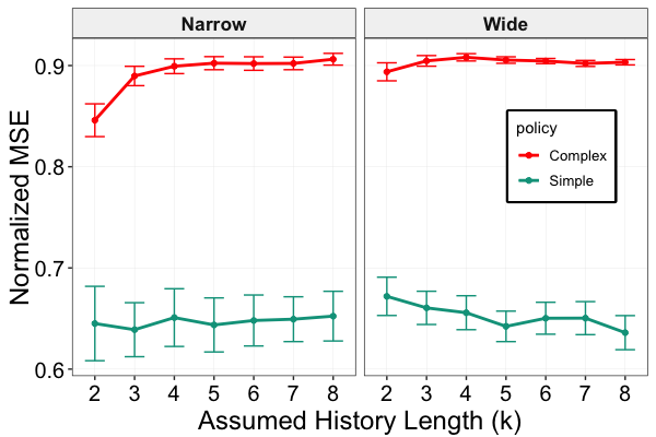
Since algorithm  1 needs to know the parameters $r$ and $k$, we first observe how sensitive it is to the choice of the assumed rank parameter $r$ and the assumed length of the history $k$. Figure  3 plots the normalized mean squared error (MSE) for various choices of $r$ and $k$ values for the two types of policies. As rank $r$ increases, the error goes down significantly. This implies that even though a tensor of rank $10$ is used in the outcome model, a tensor of higher rank might be a better fit for the marginal outcomes. On the other hand, the error seems to be quite robust to changes in the parameter $k$. However, we believe that one should see a drop in the error with higher $k$ if the outcome model is more heterogeneous e.g. the tensor $\mathbf{T}$ is more dominant in the outcome model  (10).

Finally, we fit traditional MSM [25] at every time-step $t$. Since, conditioned on the covariates and treatments, the outcome is distributed according to a normal distribution , we use a linear function as the link function, i.e., $g(a_{i,1:t},\beta^{t})=\left\langle a_{i,1:t},\beta^{t}\right\rangle$ in eq. 3. Then we solve a weighted least squares regression problem to obtain the parameters $\{\beta^{t}\}_{t\in[T]}$. For the narrow world ($N=500$ and $T=10$), MSM performs reasonably well, and the normalized MSE turns out to be 8.69 (resp. 8.31) for the simple (resp. complex) policy. Algorithm 1, on the other hand, gives much better performance and has normalized MSE of 0.64 (resp. 0.90) for the simple (resp. complex) policy with parameters $r=10$ and $k=5$. We also evaluated classical MSM on the wide world ($N=10$ and $T=500$), but it performs poorly and has normalized MSE greater than $10^{6}$. This highlights a main drawback of the MSM – traditional methods don’t perform well if the number of time-steps $T$ is large compared to $N$.

5 Conclusion and Future Work

In this work, we proposed a new type of marginal structural models based on tensors, and showed how to estimate the parameters of the model. There are many interesting directions for future work. We assumed perfect knowledge of the policies in order to estimate the weights. So, it would be interesting to learn the weights from data and develop a doubly robust estimator [5], which works if either the outcome or the treatment model is mis-specified. Furthermore, an interesting direction is to consider the presence of unobserved confounders along the lines of Bica et al. [7], who developed a deconfounder for time-varying treatments. Finally, it will be interesting to see if we can generalize the results of [12] and theoretically analyze the performance of algorithm 1.

Appendix A Proof of Theorem 1

Proof.

Let $S(i,t)$ be the random variable which denotes the length $k$-history of user $i$ at time $t$. Then, the weighted log-likelihood function with respect to a tensor $\mathbf{T}_{N,T}$ is given as :

$$L_{N,T}(\mathbf{T}_{N,T})=\frac{1}{NT}\sum_{i=1}^{N}\sum_{t=1}^{T}w_{i,t}(Y_{i,t}-\mathbf{T}_{N,T}(i,t,S(i,t)))^{2}.$$

First we compute the expected value of the weighted log-likelihood with respect to the policy $\mathscr{P}$ (i.e. the random variables $\{Y_{i,1:T}\}_{i=1}^{N},\{A_{i,1:T}\}_{i=1}^{N},\{L_{i,1:T}\}_{i=1}^{N}$ and the true underlying tensor $\mathbf{T}^{\star}_{N,T}$. We write $\ell^{*}_{N,T}(\mathbf{T}_{N,T})$ to denote this quantity as it only depends on the tensor $\mathbf{T}_{N,T}$, i.e. $\ell^{*}_{N,T}(\mathbf{T}_{N,T})=\mathrm{E}_{\mathscr{P},\mathbf{T}^{\star}_{N,T}}\left[L_{N,T}(\mathbf{T}_{N,T})\right]$.

We want to show that $\lVert\widehat{\mathbf{T}}_{N,T}-\mathbf{T}^{\star}_{N,T}\rVert$ becomes small as either $N$ or $T$ increases. Our proof is based on the proof of the consistency of the maximum likelihood given in [20]. We write $\Theta_{N,T}$ to denote the parameter space $\{\mathbf{T}\in\mathbb{R}^{T\times N\times 2^{k}}:\mathrm{rank}(\mathbf{T})\leqslant r,\lVert\mathbf{T}\rVert_{\infty}\leqslant L\}$. $\Theta_{N,T}$ is bounded but need not be closed because of issues with border tensor. It is known that there might exist a sequence of rank $r$ tensors whose limit is a rank $r+1$ tensor [8]. However, we can exploit the convexity of $L_{N,T}(\cdot)$ to overcome this problem.

First consider a neighborhood $\mathscr{B}$ of radius $d$ centered at $\mathbf{T}^{\star}_{N,T}$ and contained within the interior of $\Theta_{N,T}$.

$$\mathscr{B}=\{\mathbf{T}\in\mathbb{R}^{N\times T\times B}:\lVert\mathbf{T}-\mathbf{T}^{\star}_{N,T}\rVert_{2}/\sqrt{NT}\leqslant d\}$$

Lemma 5 proves that $L_{N,T}(\cdot)$ is convex over $\Theta_{N,T}$. Since a convex function is continuous over the interior of its domain, $L_{N,T}(\cdot)$ is continuous over $\mathscr{B}$. Moreove, unlike $\Theta_{N,T}$, set $\mathscr{B}$ is a compact set. This implies that there exists a minimizer for $L_{N,T}(\cdot)$ over $\mathscr{B}$. Suppose $\widetilde{\mathbf{T}}_{N,T}$ be the minimizer of $L_{N,T}(\cdot)$ over $\mathscr{B}$. Consider any $\mathbf{T}\in\Theta_{N,T}\setminus\mathscr{B}$. Then there exists $\lambda<1$ such that $\mathbf{T}^{\prime}=\lambda\widetilde{\mathbf{T}}_{N,T}+(1-\lambda)\mathbf{T}$ and $\mathbf{T}^{\prime}\in\mathscr{B}$. This gives us the following :

$$L_{N,T}(\widetilde{\mathbf{T}}_{N,T})\leqslant L_{N,T}(\mathbf{T}^{\prime})=L_{N,T}(\lambda\widetilde{\mathbf{T}}_{N,T}+(1-\lambda)\mathbf{T})\leqslant\lambda L_{N,T}(\widetilde{\mathbf{T}}_{N,T})+(1-\lambda)L_{N,T}(\mathbf{T})$$

$$\Rightarrow L_{N,T}(\widetilde{\mathbf{T}}_{N,T})\leqslant L_{N,T}(\mathbf{T})$$

This first line uses the convexity of $L_{N,T}(\cdot)$ (lemma 5). This proves that $\widetilde{\mathbf{T}}_{N,T}$ is actually the minimizer of $L_{N,T}(\cdot)$ over the entire parameter space $\Theta_{N,T}$. Moreover, any other minimizer of $L_{N,T}(\cdot)$ must be inside $\mathscr{B}$. Otherwise, suppose $\mathbf{T}^{\prime\prime}$ minimizes $L_{N,T}(\cdot)$ and $\mathbf{T}^{\prime\prime}\in\Theta_{N,T}\setminus\mathscr{B}$. Then for any $0<p<1$ and $\varepsilon=\delta^{2k}d^{2}$ we have with probability at least $1-O\left(1/\varepsilon^{2}N^{p}\right)$,

$$L_{N,T}(\widetilde{\mathbf{T}}_{N,T})-\varepsilon/3<L_{N,T}(\mathbf{T}^{\star}_{N,T})-\varepsilon/3<\ell^{*}_{N,T}(\mathbf{T}^{\star}_{N,T})<\ell^{*}_{N,T}(\mathbf{T}^{\prime\prime})-\varepsilon<L_{N,T}(\mathbf{T}^{\prime\prime})-2\varepsilon/3$$

The second and the fourth inequality uses lemma 1 and the third inequality uses lemma 6. Therefore, with probability at least $1-O\left(1/(d^{4}\delta^{4k}N^{p})\right)$ all the maximizers of $L_{N,T}(\cdot)$ must be inside the ball $\mathscr{B}$ as long as $k=O\left(\log_{1/\delta}N\right)$. This proves that for any $d$ we can choose $N$ large enough (possibly dependent on $\delta$) such that with probability at least $1-1/\textrm{poly}(N)$ the minimizer of $L_{N,T}(\cdot)$ lies within a $d$ neighborhood of $\mathbf{T}^{\star}_{N,T}$. This proves the consistency of the estimate when $N$ increases to inifinity. The proof of consistency when the number of time periords $T$ increases to infinity is similar.

∎

Appendix B Proof of theorem 2

Proof.

Lemma 9 shows that $\widecheck{\mathbf{T}}_{N,T}$ apporximately optimizes the original objective 5 i.e.

$$\frac{1}{NT}\sum_{p=1}^{2^{k}}\sum_{(i,t)\in S_{p}}w_{i,t}\left(Y_{i,t}-\widecheck{\mathbf{T}}_{N,T}(i,t,p)\right)^{2}\leqslant\textrm{OPT}+o_{p}(1)$$

where the error term $o_{p}(1)$ term goes to zero as $N$ goes to infinity. Now we proceed similar to the proof of theorem 1.

We write $\Theta_{N,T}$ to denote the parameter space i.e. $\{\mathbf{T}\in\mathbb{R}^{T\times N\times 2^{k}}:\mathrm{rank}(\mathbf{T})\leqslant r,\lVert\mathbf{T}\rVert_{\infty}\leqslant L\}$. First consider a neighborhood $\mathscr{B}$ of radius $d$ centered at $\mathbf{T}^{\star}_{N,T}$ and contained within the interior of $\Theta_{N,T}$.

$$\mathscr{B}=\{\mathbf{T}\in\mathbb{R}^{N\times T\times B}:\lVert\mathbf{T}-\mathbf{T}^{\star}_{N,T}\rVert_{2}/\sqrt{NT}\leqslant d\}$$

Suppose $\widetilde{\mathbf{T}}_{N,T}$ is an approximate minimizer of $L_{N,T}(\cdot)$ over $\mathscr{B}$, i.e.

$$L_{N,T}(\widetilde{\mathbf{T}}_{N,T})\leqslant\min_{\mathbf{T}\in\mathscr{B}}L_{N,T}(\mathbf{T})+o_{p}(1)$$

Consider any $\mathbf{T}\in\Theta_{N,T}\setminus\mathscr{B}$. Then there exists $\lambda<1$ such that $\mathbf{T}^{\prime}=\lambda\widetilde{\mathbf{T}}_{N,T}+(1-\lambda)\mathbf{T}$ and $\mathbf{T}^{\prime}\in\mathscr{B}$. This gives us the following :

$$L_{N,T}(\widetilde{\mathbf{T}}_{N,T})\leqslant L_{N,T}(\mathbf{T}^{\prime})+o_{p}(1)=L_{N,T}(\lambda\widetilde{\mathbf{T}}_{N,T}+(1-\lambda)\mathbf{T})+o_{p}(1)$$

$$\leqslant\lambda L_{N,T}(\widetilde{\mathbf{T}}_{N,T})+(1-\lambda)L_{N,T}(\mathbf{T})+o_{p}(1)$$

$$\Rightarrow L_{N,T}(\widetilde{\mathbf{T}}_{N,T})\leqslant L_{N,T}(\mathbf{T})+o_{p}(1)$$

This first line uses the convexity of $L_{N,T}(\cdot)$ (lemma 5). This proves that $\widetilde{\mathbf{T}}_{N,T}$ is actually an approximate minimizer of $L_{N,T}(\cdot)$ over the entire parameter space $\Theta_{N,T}$. Moreover, any other any other approximate minimizer of $L_{N,T}(\cdot)$ must be inside $\mathscr{B}$. Otherwise, suppose $\mathbf{T}^{\prime\prime}$ approximately minimizes $L_{N,T}(\cdot)$ and $\mathbf{T}^{\prime\prime}\in\Theta_{N,T}\setminus\mathscr{B}$. Then for $\varepsilon=\delta^{2k}d^{2}$ we have with probability at least $1-O\left(1/\varepsilon^{2}N^{p}\right)$,

$$L_{N,T}(\widetilde{\mathbf{T}}_{N,T})-\varepsilon/3<L_{N,T}(\mathbf{T}^{\star}_{N,T})+o_{p}(1)-\varepsilon/3<\ell^{*}_{N,T}(\widetilde{\mathbf{T}}_{N,T})+o_{p}(1)$$

$$<\ell^{*}_{N,T}(\mathbf{T}^{\prime\prime})-\varepsilon+o_{p}(1)<L_{N,T}(\mathbf{T}^{\prime\prime})-2\varepsilon/3+o_{p}(1)$$

The second and the fourth inequality uses lemma 1 and the third inequality uses lemma 6. This gives us the following:

$$L_{N,T}(\widetilde{\mathbf{T}}_{N,T})<L_{N,T}(\mathbf{T}^{\prime\prime})-\varepsilon/3+o_{p}(1)$$

As $\varepsilon$ is independent of $N$, this tells us that $\mathbf{T}^{\prime\prime}$ cannot be an approximate minimizer of $L_{N,T}(\cdot)$. Therefore, with probability at least $1-O\left(1/(d^{4}\delta^{4k}N^{p})\right)$ all the approximate minimizers of $L_{N,T}(\cdot)$ must be inside the ball $\mathscr{B}$. This proves that as long as $k=O\left(\log_{1/\delta}T\right)$, for any $d$ we can choose $N$ large enough (possibly dependent on $\delta$) such that with probability at least $1-1/\textrm{poly}(N)$ any approximate minimizer of $L_{N,T}(\cdot)$ lies within a $d$ neighborhood of $\mathbf{T}^{\star}_{N,T}$. The proof when $N$ if fixed and $T$ increases to infinity is similar if we use the second part of lemma 9. ∎

Appendix C A $(1+\varepsilon)$-multiplicative approximation

In this section, we provide the details of the $(1+\varepsilon)$-approximation algorithm for weighted tensor approximation. We will write $B$ to denote $2^{k}$. As input, we are given a tensor $\mathbf{T}\in\mathbb{R}^{N\times T\times B}$, a weight tensor $W\in\mathbb{R}^{N\times T\times B}$ and our goal is to solve

$$\min_{\begin{subarray}{c}B:\mathrm{rank}(B)\leqslant r\\ \lVert B\rVert_{\star}\leqslant L\end{subarray}}\lVert\mathbf{T}-B\rVert^{2}_{W}$$ (11)

Suppose we are guaranteed that $W$ has $s$ distinct rows and $s$ distinct columns. This also guarantees that the number of distinct tubes of $s$ is at most $S=2^{O\left(s\log s\right)}$.

Algorithm 2 Weighted Low Rank Tensor Approximation

1:  Input: Tensor $\mathbf{T}\in\mathbb{R}^{N\times T\times B}$, weight tensor $W\in\mathbb{R}^{N\times T\times B}$, rank $r$, rank of weight tensor $s$, and $\varepsilon$.

2:  Output: Tensor $\mathbf{T}^{\prime}$ of rank $k$ such that $\lVert\mathbf{T}-\mathbf{T}^{\prime}\rVert^{2}_{W}\leqslant(1+\varepsilon)\min_{B:\mathrm{rank}(B)\leqslant r,\lVert\mathbf{T}\rVert_{\star}\leqslant L}\lVert\mathbf{T}-B\rVert^{2}_{W}.$

3:  for $j=1$ to $3$ do

4:     $s_{j}\leftarrow O\left(r/\varepsilon\right)$

5:  end for

6:  Choose three sketching matrices $S_{1}\in\mathbb{R}^{TB\times s_{1}},S_{2}\in\mathbb{R}^{NB\times s_{2}}$, and $S_{3}\in\mathbb{R}^{NT\times s_{3}}$

7:  for $j=1$ to $2$ do

8:     {Omitting the third dimension}

9:     for $i=1$ to $s$ do

10:        Create $r\times s_{j}$ variables for matrix $P_{i,j}\in\mathbb{R}^{r\times s_{j}}$

11:        Set $(\hat{U}_{j})^{i}=\mathbf{T}^{j}_{i}D_{W^{j}_{i}}S_{j}P^{T}_{j,i}(P_{j,i}P^{T}_{j,i})^{-1}$

12:     end for

13:  end for

14:  for $i=1$ to $S$ do

15:     {Representing the third dimension}

16:     Set $(\hat{U}_{3})^{i}=\mathbf{T}^{3}_{i}D_{W^{3}_{i}}S_{j}P^{T}_{3,i}(P_{3,i}P^{T}_{3,i})^{-1}$

17:  end for

18:  Form $\lVert W\cdot(\hat{U}_{1}\otimes\hat{U}_{2}\otimes\hat{U}_{3}-\mathbf{T})\rVert^{2}_{F}$

19:  for $i=1$ to $r$ do

20:     Add constraint $\lVert\hat{U}_{1}^{i}\rVert^{2}_{2}\lVert\hat{U}_{2}^{i}\rVert^{2}_{2}\lVert\hat{U}_{3}^{i}\rVert^{2}_{2}\leqslant L$

21:  end for

22:  Run Polynomial System Verifier to get $U_{1},U_{2},$ and $U_{3}$

23:  

24:  return  $U_{1}\otimes U_{2}\otimes U_{3}$

Algorithm 2 closely follows algorithm G.4 in [31] with modifications to handle asymmetric tensors and additional constraint on the bound for the largest singular value. It chooses three sketching matrices of appropriate dimension to solve the original low-rank approximation problem in a low-dimensional space. The main idea is that the entries of $\hat{U}_{1}$ can be repersented with as polynomials of the variables for $i=1$ to $s$ (line 10). This is possible because the weight matrix has $s$ distinct rows and columns, which implies that it’s flatenning along the rows has $s$ distinct faces. The same thing holds for $\hat{U}_{2}$. However, this need not be true for $\hat{U}_{3}$, so they are represented through $S$ distinct denominators (line 16). With this setup [31] shows that the number of variables in the polynomial system verifier is $O\left(r^{2}s/\varepsilon\right)$ and the number of constraints is $2s+S$. In line 18, we add additional $r$ constraints. So the total number of constraints is $2s+r+2^{O\left(s\log s\right)}$ and the total number of variables is $O\left(r^{2}s/\varepsilon\right)$. Moreover, the degree of the new constraints in line 18 is at most $\textrm{poly}(r,s,S)$. A polynomial system can be verified in time $(\text{\# max degree of any polynomial})^{\text{\# number of variables}}$. In our case, this takes time

$$\left(\textrm{poly}(r,s)\textrm{poly}\left(2^{O\left(s\log s\right)}\right)\right)^{O\left(r^{2}s/\varepsilon\right)}=\left(\textrm{poly}(r,s)2^{O\left(s\log s\right)}\right)^{O\left(r^{2}s/\varepsilon\right)}=2^{\tilde{O}\left(r^{2}s^{2}/\varepsilon\right)}.$$

Recall that we want to compute a low-rank approximation of the tensor $Y_{w}\in\mathbb{R}^{N\times T\times 2^{k}}$. Although $\mathit{nnz}(Y_{w})=NT$, positivity implies that the number of nonzero entries in $W$ is $\mathit{nnz}(W)=NT2^{k}$. Therefore, the resulting algorithm runs in time time $O\left(NT2^{k}+\max\{N,T,2^{k}\}2^{\tilde{O}\left(s^{2}r^{2}/\varepsilon\right)}\right)$ and outputs a tensor $\widetilde{\mathbf{T}}_{N,T}$ such that $\lVert Y_{w}-\widetilde{\mathbf{T}}_{N,T}\rVert^{2}_{W}\leqslant(1+\varepsilon)\min_{\mathbf{T}\in\mathbb{R}^{N\times T\times 2^{k}},\mathrm{rank}(\mathbf{T})\leqslant r}\lVert Y_{w}-\mathbf{T}\rVert^{2}_{W}$ with probability at least $9/10$.

C.1 Distinct Faces of the Weight Matrix

Recall that we need the weight matrix $W$ to have $s$ distinct faces in two dimensions, where the weight matrix $W$ is defined as $W(i,t,p)=\sqrt{\mathrm{Pr}\left[(i,t)\in O_{p}\right]}$. If the underlying policy satisfies the following two assumptions, then the matrix $W$ has $s$ distinct faces along the two dimensions.

1. There are $s$ groups of subjects such that the policy treats all the subjects in a group identically.

2. There are $s$ groups of time periods such that for any two time $t$ and $t^{\prime}$ belonging to the same group we have the same marginal probabilities across all the subjects ($\mathrm{Pr}\left[(i,t)\in O_{p}\right]=\mathrm{Pr}\left[(i,t^{\prime})\in O_{p}\right]\ \forall i,p$).

These two assumptions together imply that $W$ has $s$ distinct faces in two dimensions, and allows an efficient $(1+\varepsilon)$-multiplicative approximation of the tensor approximation problem defined in equation 11.

Appendix D Additional Lemmata

Lemma 1.

Suppose $\mathbf{T}^{\star}_{N,T}$ exists for all $N$ and $T$.

• If $k\leqslant O\left(\log_{(1-\delta)/\delta}N\right)$, $\mathrm{Pr}\left[\left|L_{N,T}(\mathbf{T})-\ell^{*}_{N,T}(\mathbf{T})\right|>\varepsilon\right]\rightarrow 0$ as $N\rightarrow\infty$.

• If $k\leqslant O\left(\log_{(1-\delta)/\delta}N\right)$, and A.2 holds $\mathrm{Pr}\left[\left|L_{N,T}(\mathbf{T})-\ell^{*}_{N,T}(\mathbf{T})\right|>\varepsilon\right]\rightarrow 0$ as $T\rightarrow\infty$.

Proof.

We will write $S(i,t)$ to denote the history of length $k$ for user $i$ at time $t$. With this notation, our objective function becomes,

$$L_{N,T}(\mathbf{T})=\frac{1}{NT}\sum_{i,t}w_{i,t}\left(Y_{i,t}-\mathbf{T}(i,t,S(i,t))\right)^{2}$$

$$\mathrm{Pr}\left[\left|L_{N,T}(\mathbf{T})-\ell^{*}_{N,T}(\mathbf{T})\right|>\varepsilon\right]\leqslant\frac{\mathrm{Var}\left(L_{N,T}(\mathbf{T})\right)}{\varepsilon^{2}}=\frac{1}{\varepsilon^{2}N^{2}T^{2}}\mathrm{Var}\left(\sum_{i,t}w_{i,t}\left(Y_{i,t}-\mathbf{T}(i,t,S(i,t))\right)^{2}\right)$$

$$=\frac{1}{\varepsilon^{2}N^{2}T^{2}}\left[\sum_{i,t}\mathrm{Var}\left(w_{i,t}\left(Y_{i,t}-\mathbf{T}(i,t,S(i,t))\right)^{2}\right)\right.$$

$$+\left.2\sum_{i,t<t^{\prime}}\textrm{cov}\left(w_{i,t}\left(Y_{i,t}-\mathbf{T}(i,t,S(i,t))\right)^{2},w_{i,t^{\prime}}\left(Y_{i,t}-\mathbf{T}(i,t^{\prime},S(i,t^{\prime}))\right)^{2}\right)\right]$$

$$\leqslant\frac{1}{\varepsilon^{2}N^{2}T^{2}}\left[\sum_{i,t}\mathrm{E}\left[w^{2}_{i,t}\left(Y_{i,t}-\mathbf{T}(i,t,S(i,t))\right)^{4}\right]\right.$$

$$+2\left.\sum_{i,t<t^{\prime}\leqslant t+k}\mathrm{E}\left[w_{i,t}w_{i,t^{\prime}}\left(Y_{i,t}-\mathbf{T}(i,t,S(i,t))\right)^{2}\left(Y_{i,t^{\prime}}-\mathbf{T}(i,t^{\prime},S(i,t^{\prime}))\right)^{2}\right]\right.$$

$$+\left.2\sum_{i,t+k<t^{\prime}}\textrm{cov}\left(w_{i,t}\left(Y_{i,t}-\mathbf{T}(i,t,S(i,t))\right)^{2},w_{i,t^{\prime}}\left(Y_{i,t^{\prime}}-\mathbf{T}(i,t^{\prime},S(i,t^{\prime}))\right)^{2}\right)\right]$$

Now we bound each term in the last summation. First, consider the case when $T$ is fixed and $N$ goes to infinity. Since weightes are bounded by $\left(\frac{1-\delta}{\delta}\right)^{k}$ and the fourth moments of the counterfactual outcomes are bounded, there exists a constant $M_{1}>0$ such that $\mathrm{E}\left[w^{2}_{i,t}\left(Y_{i,t}-\mathbf{T}(i,t,S(i,t))\right)^{4}\right]\leqslant\left(\frac{1-\delta}{\delta}\right)^{2k}M_{1}$. By a similar argument we can bound the second term $\mathrm{E}\left[w_{i,t}w_{i,t^{\prime}}\left(Y_{i,t}-\mathbf{T}(i,t,S(i,t))\right)^{2}\left(Y_{i,t^{\prime}}-\mathbf{T}(i,t^{\prime},S(i,t^{\prime}))\right)^{2}\right]$ by $\left(\frac{1-\delta}{\delta}\right)^{2k}M_{1}$. Finally, we can bound the covariance term by the expectation of the products and get a similar bound. This gives us the following bound on the probability:

$$\mathrm{Pr}\left[\left|L_{N,T}(\mathbf{T})-\ell^{*}_{N,T}(\mathbf{T})\right|>\varepsilon\right]\leqslant\frac{1}{\varepsilon^{2}N^{2}T^{2}}\left[NTM_{1}\left(\frac{1-\delta}{\delta}\right)^{2k}+2NT^{2}M_{1}\left(\frac{1-\delta}{\delta}\right)^{2k}\right]$$

$$=O\left(\frac{1}{\varepsilon^{2}N^{p}}\right)$$

for any $0<p<1$ as long as $k=O\left((1-p)\log_{(1-\delta)/\delta}N\right)$. This gives us the first result.

Now consider the case when $T$ increases to infinity and $N$ is fixed. As before we bound $\mathrm{E}\left[w^{2}_{i,t}\left(Y_{i,t}-\mathbf{T}(i,t,S(i,t))\right)^{4}\right]$ by $\left(\frac{1-\delta}{\delta}\right)^{2k}M_{1}$. When $t<t^{\prime}\leqslant t+k$ we bound $\mathrm{E}\left[w_{i,t}w_{i,t^{\prime}}\left(Y_{i,t}-\mathbf{T}(i,t,S(i,t))\right)^{2}\left(Y_{i,t^{\prime}}-\mathbf{T}(i,t^{\prime},S(i,t^{\prime}))\right)^{2}\right]$ by $\left(\frac{1-\delta}{\delta}\right)^{2k}M_{1}$ and there are $Tk$ such terms. On the other hand, if $t^{\prime}>t+k$ and A.2 holds lemma 10 proves a bound of $O(\left(t^{\prime}-t\right)^{1-\gamma})$ on the covariance term. This gives us the following bound on the probability:

$$\mathrm{Pr}\left[\left|L_{N,T}(\mathbf{T})-\ell^{*}_{N,T}(\mathbf{T})\right|>\varepsilon\right]\leqslant\frac{1}{\varepsilon^{2}N^{2}T^{2}}\left[NTM_{1}\left(\frac{1-\delta}{\delta}\right)^{2k}+2kTM_{1}\left(\frac{1-\delta}{\delta}\right)^{2k}+\sum_{t:t^{\prime}>t+k}c\left(t^{\prime}-t\right)^{1-\gamma}\right]$$

$$=O\left(\frac{1}{\varepsilon^{2}T^{p}}\right)$$

for any $0<p<\gamma$ as long as $k=O\left((1-p)\log_{(1-\delta)/\delta}N\right)$. This establishes the second result. ∎

Lemma 2.

$$\mathrm{E}_{H_{i,1:t}}\left[w_{i,t}(Y_{i,t}-\mathbf{T}(i,t,S(i,t))^{2})\right]=\sum_{A_{i,t-k+1:t}}\mathrm{Pr}\left[A_{i,t-k+1:t}\right]^{2}\sum_{L_{i,1:t}}\mathrm{Pr}\left[L_{i,1:t}|A_{i,t-k+1:t}\right]\times$$

$$\sum_{Y_{i,t}}\mathrm{Pr}\left[Y_{i,t}|A_{i,t-k+1:t},L_{i,1:t}\right]\left(Y_{i,t}(A_{i,t-k+1:t},L_{i,1:t})-\mathbf{T}(i,t,A_{i,t-k+1:t})\right)^{2}$$

Proof.

We assume that the outcome variable is discrete. The proof for continuous variable is similar.

$$\mathrm{E}_{H_{i,1:t}}\left[w_{i,t}(Y_{i,t}-\mathbf{T}(i,t,S(i,t))^{2})\right]$$

$$=\sum_{A_{i,1:t}}\sum_{L_{i,1:t}}\sum_{Y_{i,1:t}}\mathrm{Pr}\left[A_{i,1:t},L_{i,1:t},Y_{i,1:t}\right]\prod_{s=t-k+1}^{t}\frac{\mathrm{Pr}\left[A_{i,s}|A_{i,t-k+1:s-1}\right]}{\mathrm{Pr}\left[A_{i,s}|A_{i,t-k+1:s-1},L_{i,1:s}\right]}\times$$

$$\left(Y_{i,t}(A_{i,t-k+1:t},L_{i,1:t})-\mathbf{T}(i,t,A_{i,t-k+1:t})\right)^{2}$$

$$=\sum_{A_{i,1:t}}\sum_{L_{i,1:t}}\sum_{Y_{i,1:t}}\mathrm{Pr}\left[A_{i,1:t},L_{i,1:t},Y_{i,1:t}\right]\frac{\mathrm{Pr}\left[A_{i,t-k+1:t}\right]}{\mathrm{Pr}\left[A_{i,t-k+1:t}|L_{i,1:t}\right]}\times$$

$$\left(Y_{i,t}(A_{i,t-k+1:t},L_{i,1:t})-\mathbf{T}(i,t,A_{i,t-k+1:t})\right)^{2}$$

$$=\sum_{A_{i,t-k+1:t}}\sum_{L_{i,1:t}}\sum_{Y_{i,t}}\mathrm{Pr}\left[A_{i,t-k+1:t},L_{i,1:t},Y_{i,t}\right]\frac{\mathrm{Pr}\left[A_{i,t-k+1:t}\right]}{\mathrm{Pr}\left[A_{i,t-k+1:t}|L_{i,1:t}\right]}\times$$

$$\left(Y_{i,t}(A_{i,t-k+1:t},L_{i,1:t})-\mathbf{T}(i,t,A_{i,t-k+1:t})\right)^{2}$$

$$=\sum_{A_{i,t-k+1:t}}\sum_{L_{i,1:t}}\sum_{Y_{i,t}}\mathrm{Pr}\left[A_{i,t-k+1:t}\right]\mathrm{Pr}\left[L_{i,1:t}\right]\mathrm{Pr}\left[Y_{i,t}|A_{i,t-k+1:t},L_{i,1:t}\right]\times$$

$$\left(Y_{i,t}(A_{i,t-k+1:t},L_{i,1:t})-\mathbf{T}(i,t,A_{i,t-k+1:t})\right)^{2}$$

$$=\sum_{A_{i,t-k+1:t}}\mathrm{Pr}\left[A_{i,t-k+1:t}\right]^{2}\sum_{L_{i,1:t}}\mathrm{Pr}\left[L_{i,1:t}|A_{i,t-k+1:t}\right]\sum_{Y_{i,t}}\mathrm{Pr}\left[Y_{i,t}|A_{i,t-k+1:t},L_{i,1:t}\right]\times$$

$$\left(Y_{i,t}(A_{i,t-k+1:t},L_{i,1:t})-\mathbf{T}(i,t,A_{i,t-k+1:t})\right)^{2}$$

∎

Lemma 3.

$w_{i,t}\leqslant\left(\frac{1-\delta}{\delta}\right)^{k}$

Proof.

$$w_{i,t}=\prod_{s=t-k+1}^{t}\frac{\mathrm{Pr}\left[A_{i,s}|A_{i,t-k+1:s-1}\right]}{\mathrm{Pr}\left[A_{i,s}|A_{i,t-k+1:s-1},L_{i,1:s}\right]}$$

Recall that the given policy satisfies positivity with constant $\delta$ i.e. for each $A_{i,1:s-1},L_{i,1:s},Y_{i,1:s-1}$, we have

$$\delta<\mathrm{Pr}\left[A_{i,s}|A_{i,1:s-1},L_{i,1:s}\right]<1-\delta$$

First, consider the term in the denominator.

$$\mathrm{Pr}\left[A_{i,s}|A_{i,t-k+1:s-1},L_{i,1:s}\right] =\sum_{A_{i,1:t-k}}\mathrm{Pr}\left[A_{i,1:t-k}|L_{i,1:s-1}\right]\mathrm{Pr}\left[A_{i,s}|A_{i,1:s-1},L_{i,1:s}\right]$$

$$\geqslant\delta\sum_{A_{i,1:t-k}}\mathrm{Pr}\left[A_{i,1:t-k}|L_{i,1:s-1}\right]=\delta$$

This gives a lower bound of $\delta$ on the term in the denominator. Now consider the term in the numerator. Positivity implies that $\mathrm{Pr}\left[A_{i,s}|A_{i,1:s-1}\right]=\mathrm{Pr}\left[A_{i,s}|A_{i,1:s-1},L_{i,1:s},Y_{i,1:s-1}\right]\mathrm{Pr}\left[L_{i,1:s},Y_{i,1:s-1}\right]\leqslant 1-\delta$. These two results imply that each term in the product of $w_{i,t}$ is bounded by $(1-\delta)/\delta$ and we get the desired bound on $w_{i,t}$. ∎

Lemma 4.

$$\mathrm{E}_{H_{i,1:t^{\prime}}}\left[w_{i,t}w_{i,t^{\prime}}(Y_{i,t}-\mathbf{T}(i,t,S(i,t))^{2})(Y_{i,t^{\prime}}-\mathbf{T}(i,t^{\prime},S(i,t^{\prime}))^{2})\right]$$

$$=\sum_{A_{i,t-k+1:t}}\sum_{L_{i,1:t}}\sum_{Y_{i,t}}\mathrm{Pr}\left[A_{i,t-k+1:t}\right]\mathrm{Pr}\left[L_{i,1:t}\right]\mathrm{Pr}\left[Y_{i,t}|A_{i,t-k+1:t},L_{i,1:t}\right]\times$$

$$\left(Y_{i,t}(A_{i,t-k+1:t},L_{i,1:t})-\mathbf{T}(i,t,A_{i,t-k+1:t})\right)^{2}\times$$

$$\sum_{A_{i,t^{\prime}-k+1:t^{\prime}}}\sum_{L_{i,t+1:t^{\prime}}}\sum_{Y_{i,t^{\prime}}}\mathrm{Pr}\left[A_{i,t^{\prime}-k+1:t^{\prime}}\right]\mathrm{Pr}\left[A_{i,t^{\prime}-k+1:t^{\prime}}|L_{i,1:t},A_{i,t-k+1:t}\right]\times$$

$$\mathrm{Pr}\left[L_{i,t+1:t^{\prime}}|A_{i,t-k+1:t},L_{i,1:t},A_{i,t^{\prime}-k+1:t^{\prime}}\right]\times$$

$$\mathrm{Pr}\left[Y_{i,t^{\prime}}|A_{i,t^{\prime}-k+1:t^{\prime}},L_{i,1:t^{\prime}}\right]\left(Y_{i,t^{\prime}}(A_{i,t^{\prime}-k+1:t^{\prime}},L_{i,1:t^{\prime}})-\mathbf{T}(i,t^{\prime},A_{i,t^{\prime}-k+1:t^{\prime}})\right)^{2}$$

Proof.

We assume that the outcome variable is discrete. The proof for continuous variable is similar.

$$\mathrm{E}_{H_{i,1:t^{\prime}}}\left[w_{i,t}w_{i,t^{\prime}}(Y_{i,t}-\mathbf{T}(i,t,S(i,t))^{2})(Y_{i,t^{\prime}}-\mathbf{T}(i,t^{\prime},S(i,t^{\prime}))^{2})\right]$$

$$=\sum_{A_{i,1:t^{\prime}}}\sum_{L_{i,1:t^{\prime}}}\sum_{Y_{i,1:t^{\prime}}}\mathrm{Pr}\left[A_{i,1:t^{\prime}},L_{i,1:t^{\prime}},Y_{i,1:t^{\prime}}\right]\times$$

$$\prod_{s=t-k+1}^{t}\frac{\mathrm{Pr}\left[A_{i,s}|A_{i,t-k+1:s-1}\right]}{\mathrm{Pr}\left[A_{i,s}|A_{i,t-k+1:s-1},L_{i,1:s}\right]}\times\prod_{s=t-k+1}^{t}\frac{\mathrm{Pr}\left[A_{i,s}|A_{i,t-k+1:s-1}\right]}{\mathrm{Pr}\left[A_{i,s}|A_{i,t-k+1:s-1},L_{i,1:s}\right]}\times$$

$$\left(Y_{i,t}(A_{i,t-k+1:t},L_{i,1:t})-\mathbf{T}(i,t,A_{i,t-k+1:t})\right)^{2}\times\left(Y_{i,t^{\prime}}(A_{i,t^{\prime}-k+1:t^{\prime}},L_{i,1:t^{\prime}})-\mathbf{T}(i,t^{\prime},A_{i,t^{\prime}-k+1:t^{\prime}})\right)^{2}$$

$$=\sum_{A_{i,1:t^{\prime}}}\sum_{L_{i,1:t^{\prime}}}\sum_{Y_{i,1:t^{\prime}}}\mathrm{Pr}\left[A_{i,1:t^{\prime}},L_{i,1:t^{\prime}},Y_{i,1:t^{\prime}}\right]\frac{\mathrm{Pr}\left[A_{i,t-k+1:t}\right]}{\mathrm{Pr}\left[A_{i,t-k+1:t}|L_{i,1:t}\right]}\times\frac{\mathrm{Pr}\left[A_{i,t^{\prime}-k+1:t^{\prime}}\right]}{\mathrm{Pr}\left[A_{i,t^{\prime}-k+1:t^{\prime}}|L_{i,1:t^{\prime}}\right]}\times$$

$$\left(Y_{i,t}(A_{i,t-k+1:t},L_{i,1:t})-\mathbf{T}(i,t,A_{i,t-k+1:t})\right)^{2}\times\left(Y_{i,t^{\prime}}(A_{i,t^{\prime}-k+1:t^{\prime}},L_{i,1:t^{\prime}})-\mathbf{T}(i,t^{\prime},A_{i,t^{\prime}-k+1:t^{\prime}})\right)^{2}$$

$$=\sum_{A_{i,t-k+1:t}}\sum_{A_{i,t^{\prime}-k+1:t^{\prime}}}\sum_{L_{i,1:t^{\prime}}}\sum_{Y_{i,t}}\sum_{Y_{i,t^{\prime}}}\mathrm{Pr}\left[A_{i,t-k+1:t},A_{i,t^{\prime}-k+1:t^{\prime}},L_{i,1:t^{\prime}},Y_{i,t},Y_{i,t^{\prime}}\right]\times$$

$$\frac{\mathrm{Pr}\left[A_{i,t-k+1:t}\right]}{\mathrm{Pr}\left[A_{i,t-k+1:t}|L_{i,1:t}\right]}\times\frac{\mathrm{Pr}\left[A_{i,t^{\prime}-k+1:t^{\prime}}\right]}{\mathrm{Pr}\left[A_{i,t^{\prime}-k+1:t^{\prime}}|L_{i,1:t^{\prime}}\right]}\times$$

$$\left(Y_{i,t}(A_{i,t-k+1:t},L_{i,1:t})-\mathbf{T}(i,t,A_{i,t-k+1:t})\right)^{2}\times\left(Y_{i,t^{\prime}}(A_{i,t^{\prime}-k+1:t^{\prime}},L_{i,1:t^{\prime}})-\mathbf{T}(i,t^{\prime},A_{i,t^{\prime}-k+1:t^{\prime}})\right)^{2}$$

$$=\sum_{A_{i,t-k+1:t}}\sum_{L_{i,1:t}}\sum_{Y_{i,t}}\mathrm{Pr}\left[A_{i,t-k+1:t}\right]\mathrm{Pr}\left[L_{i,1:t}\right]\mathrm{Pr}\left[Y_{i,t}|A_{i,t-k+1:t},L_{i,1:t}\right]\times$$

$$\left(Y_{i,t}(A_{i,t-k+1:t},L_{i,1:t})-\mathbf{T}(i,t,A_{i,t-k+1:t})\right)^{2}\times$$

$$\sum_{A_{i,t^{\prime}-k+1:t^{\prime}}}\sum_{L_{i,t+1:t^{\prime}}}\sum_{Y_{i,t^{\prime}}}\mathrm{Pr}\left[A_{i,t^{\prime}-k+1:t^{\prime}}|L_{i,1:t},A_{i,t-k+1:t}\right]\mathrm{Pr}\left[L_{i,t+1:t^{\prime}}|A_{i,t-k+1:t},L_{i,1:t},A_{i,t^{\prime}-k+1:t^{\prime}}\right]\times$$

$$\frac{\mathrm{Pr}\left[L_{i,1:t^{\prime}}\right]}{\mathrm{Pr}\left[L_{i,1:t^{\prime}}|A_{i,t^{\prime}-k+1:t^{\prime}}\right]}\times$$

$$\mathrm{Pr}\left[Y_{i,t^{\prime}}|A_{i,t^{\prime}-k+1:t^{\prime}},L_{i,1:t^{\prime}}\right]\left(Y_{i,t^{\prime}}(A_{i,t^{\prime}-k+1:t^{\prime}},L_{i,1:t^{\prime}})-\mathbf{T}(i,t^{\prime},A_{i,t^{\prime}-k+1:t^{\prime}})\right)^{2}$$

$$=\sum_{A_{i,t-k+1:t}}\sum_{L_{i,1:t}}\sum_{Y_{i,t}}\mathrm{Pr}\left[A_{i,t-k+1:t}\right]\mathrm{Pr}\left[L_{i,1:t}\right]\mathrm{Pr}\left[Y_{i,t}|A_{i,t-k+1:t},L_{i,1:t}\right]\times$$

$$\left(Y_{i,t}(A_{i,t-k+1:t},L_{i,1:t})-\mathbf{T}(i,t,A_{i,t-k+1:t})\right)^{2}\times$$

$$\sum_{A_{i,t^{\prime}-k+1:t^{\prime}}}\sum_{L_{i,t+1:t^{\prime}}}\sum_{Y_{i,t^{\prime}}}\mathrm{Pr}\left[A_{i,t^{\prime}-k+1:t^{\prime}}\right]\mathrm{Pr}\left[A_{i,t^{\prime}-k+1:t^{\prime}}|L_{i,1:t},A_{i,t-k+1:t}\right]\times$$

$$\mathrm{Pr}\left[L_{i,t+1:t^{\prime}}|A_{i,t-k+1:t},L_{i,1:t},A_{i,t^{\prime}-k+1:t^{\prime}}\right]\times$$

$$\mathrm{Pr}\left[Y_{i,t^{\prime}}|A_{i,t^{\prime}-k+1:t^{\prime}},L_{i,1:t^{\prime}}\right]\left(Y_{i,t^{\prime}}(A_{i,t^{\prime}-k+1:t^{\prime}},L_{i,1:t^{\prime}})-\mathbf{T}(i,t^{\prime},A_{i,t^{\prime}-k+1:t^{\prime}})\right)^{2}$$

∎

Lemma 5.

$L_{N,T}(\mathbf{T})$ is convex in $\mathbf{T}$.

Proof.

$$L_{N,T}(\mathbf{T}) =\frac{1}{NT}\sum_{i=1}^{N}\sum_{t=1}^{T}w_{i,t}(Y_{i,t}-\mathbf{T}(i,t,S(i,t)))^{2}$$

Each term inside the summation i.e. $(Y_{i,t}-\mathbf{T}_{N,T}(i,t,S(i,t)))^{2}$ is a convex function. The likelihood function is a non-negative weighted sum of convex functions and is also convex. ∎

Lemma 6.

Let $\mathscr{N}$ be a $d$-neighborhood of $\mathbf{T}^{\star}_{N,T}$ i.e. $\mathscr{N}=\{\mathbf{T}:\lVert\mathbf{T}^{\star}_{N,T}-\mathbf{T}\rVert_{2}/\sqrt{NT}\leqslant d\}$. Then for any $\mathbf{T}^{\prime}\notin\mathscr{N}$ we have $\ell^{*}_{N,T}(\mathbf{T}^{\star}_{N,T})<\ell^{*}_{N,T}(\mathbf{T}^{\prime})-\delta^{2k}d^{2}$.

Proof.

Lemma 2 gives us

$$\ell^{*}_{N,T}(\mathbf{T}^{\star}_{N,T})-\ell^{*}_{N,T}(\mathbf{T}^{\prime})$$

$$=\frac{1}{NT}\sum_{i,t}\sum_{A_{i,t-k+1:t}}\mathrm{Pr}\left[A_{i,t-k+1:t}\right]^{2}\sum_{L_{i,1:t}}\mathrm{Pr}\left[L_{i,1:t}|A_{i,t-k+1:t}\right]\sum_{Y_{i,t}}\mathrm{Pr}\left[Y_{i,t}|A_{i,t-k+1:t},L_{i,1:t}\right]\times$$

$$\left(Y_{i,t}(A_{i,t-k+1:t},L_{i,1:t})-\mathbf{T}^{\star}_{N,T}(i,t,A_{i,t-k+1:t})\right)^{2}-\left(Y_{i,t}(A_{i,t-k+1:t},L_{i,1:t})-\mathbf{T}^{\prime}(i,t,A_{i,t-k+1:t})\right)^{2}$$

$$=\sum_{A_{i,t-k+1:t}}\mathrm{Pr}\left[A_{i,t-k+1:t}\right]^{2}\sum_{L_{i,1:t}}\mathrm{Pr}\left[L_{i,1:t}|A_{i,t-k+1:t}\right]\sum_{Y_{i,t}}\mathrm{Pr}\left[Y_{i,t}|A_{i,t-k+1:t},L_{i,1:t}\right]\times$$

$$\left\{-2Y_{i,t}(A_{i,t-k+1:t},L_{i,1:t})(\mathbf{T}^{\star}_{N,T}(i,t,A_{i,t-k+1:t})-\mathbf{T}^{\prime}(i,t,A_{i,t-k+1:t}))\right.$$

$$+\left.(\mathbf{T}^{\star}_{N,T}(i,t,A_{i,t-k+1:t}))^{2}-(\mathbf{T}^{\prime}(i,t,A_{i,t-k+1:t}))^{2}\right\}$$

Now we use the definition of $\mathbf{T}^{\star}_{N,T}$ i.e.

$$\mathbf{T}^{\star}_{N,T}(i,t,A_{i,t-k+1:t})=\mathrm{Pr}\left[L_{i,1:t}|A_{i,t-k+1:t}\right]\sum_{Y_{i,t}}\mathrm{Pr}\left[Y_{i,t}|A_{i,t-k+1:t},L_{i,1:t}\right]Y_{i,t}(A_{i,t-k+1:t},L_{i,1:t})$$

and get

$$\ell^{*}_{N,T}(\mathbf{T}^{\star}_{N,T})-\ell^{*}_{N,T}(\mathbf{T}^{\prime})=\frac{1}{NT}\sum_{i,t}\sum_{A_{i,t-k+1:t}}\mathrm{Pr}\left[A_{i,t-k+1:t}\right]^{2}\times$$

$$\left\{-2\mathbf{T}^{\star}_{N,T}(i,t,A_{i,t-k+1:t})(\mathbf{T}^{\star}_{N,T}(i,t,A_{i,t-k+1:t})-\mathbf{T}^{\prime}(i,t,A_{i,t-k+1:t}))\right.$$

$$+\left.(\mathbf{T}^{\star}_{N,T}(i,t,A_{i,t-k+1:t}))^{2}-(\mathbf{T}^{\prime}(i,t,A_{i,t-k+1:t}))^{2}\right\}$$

$$=-\frac{1}{NT}\sum_{i,t}\sum_{A_{i,t-k+1:t}}\mathrm{Pr}\left[A_{i,t-k+1:t}\right]^{2}\left(\mathbf{T}^{\star}_{N,T}(i,t,A_{i,t-k+1:t})-\mathbf{T}^{\prime}(i,t,A_{i,t-k+1:t})\right)^{2}$$

$$\leqslant-\delta^{2k}\frac{1}{NT}\lVert\mathbf{T}^{\star}_{N,T}-\mathbf{T}^{\prime}\rVert_{2}^{2}\leqslant-\delta^{2k}d^{2}$$

The final step uses positivity and the fact that $\lVert\mathbf{T}^{\star}_{N,T}-\mathbf{T}^{\prime}\rVert_{2}/\sqrt{NT}>d$. ∎

Lemma 7.

Suppose $\lVert\mathbf{T}\rVert_{\infty}\leqslant L$. Then

$$\mathrm{Pr}\left[\left|\frac{1}{NT}\sum_{p=1}^{2^{k}}\sum_{(i,t)\in S_{p}}w_{i,t}\mathbf{T}^{2}(i,t,p)-\frac{1}{NT}\lVert\mathbf{T}\rVert_{W}^{2}\right|\geqslant\varepsilon\right]\leqslant 2\exp\left(-\frac{2N\varepsilon^{2}}{L^{4}\left(\frac{1-\delta}{\delta}\right)^{2k}}\right)$$

Proof.

Suppose $S(i,t)$ be the slice selected by the policy for agent $i$ at time $t$. Then we have $\frac{1}{NT}\sum_{p=1}^{2^{k}}\sum_{(i,t)\in S_{p}}w_{i,t}\mathbf{T}^{2}(i,t,p)=\frac{1}{NT}\sum_{i=1}^{N}\sum_{t=1}^{T}w_{i,t}\mathbf{T}^{2}(i,t,S(i,t))$. Observe that for each $i$,

$$\frac{1}{T}\sum_{t=1}^{T}w_{i,t}\mathbf{T}^{2}(i,t,S(i,t))\in\left[0,L^{2}\left(\frac{1-\delta}{\delta}\right)^{k}\right]$$

. Now we apply the Hoeffding inequality considering the random variables $\left\{\frac{1}{T}\sum_{t=1}^{T}w_{i,t}\mathbf{T}^{2}(i,t,S(i,t))\right\}_{i=1}^{N}$ as independent random variables and get the following bound.

$$\mathrm{Pr}\left[\left|\frac{1}{NT}\sum_{p=1}^{B}\sum_{(i,t)\in S_{p}}w_{i,t}\mathbf{T}^{2}(i,t,p)-\frac{1}{NT}\lVert\mathbf{T}\rVert_{W}^{2}\right|\geqslant\varepsilon\right]\leqslant 2\exp\left(-\frac{2N\varepsilon^{2}}{L^{4}\left(\frac{1-\delta}{\delta}\right)^{2k}}\right)$$ (12)

∎

Lemma 8.

Suppose $\lVert\mathbf{T}\rVert_{\infty}\leqslant L$ and A.2 holds. Then

$$\mathrm{Pr}\left[\left|\frac{1}{NT}\sum_{p=1}^{B}\sum_{(i,t)\in O_{p}}w_{i,t}\mathbf{T}^{2}(i,t,p)-\frac{1}{NT}\lVert\mathbf{T}\rVert_{W}^{2}\right|\geqslant\varepsilon\right]\leqslant O\left(\frac{L^{4}\left(\frac{1-\delta}{\delta}\right)^{2k}}{\varepsilon^{2}T^{\gamma}}\right)$$

Proof.

Suppose $S(i,t)$ be the slice selected by the policy for agent $i$ at time $t$. Then we have $\frac{1}{NT}\sum_{p=1}^{B}\sum_{(i,t)\in O_{p}}w_{i,t}\mathbf{T}^{2}(i,t,p)=\frac{1}{NT}\sum_{i=1}^{N}\sum_{t=1}^{T}w_{i,t}\mathbf{T}^{2}(i,t,S(i,t))$. Observe that for each $t$,

$$\frac{1}{N}\sum_{i=1}^{N}w_{i,t}\mathbf{T}^{2}(i,t,S(i,t))\in\left[0,L^{2}\left(\frac{1-\delta}{\delta}\right)^{k}\right]$$

. Now we apply the Chebyshev inequality considering the random variables $\left\{\frac{1}{N}\sum_{i=1}^{N}w_{i,t}\mathbf{T}^{2}(i,t,S(i,t))\right\}_{t=1}^{T}$.

$$\mathrm{Pr}\left[\left|\frac{1}{NT}\sum_{p=1}^{B}\sum_{(i,t)\in O_{p}}w_{i,t}\mathbf{T}^{2}(i,t,p)-\frac{1}{NT}\lVert\mathbf{T}\rVert_{W}^{2}\right|\geqslant\varepsilon\right]\leqslant\frac{\mathrm{Var}\left(\frac{1}{NT}\sum_{t=1}^{T}\sum_{i=1}^{N}w_{i,t}\mathbf{T}^{2}(i,t,S(i,t))\right)}{\varepsilon^{2}}$$

$$=\frac{1}{\varepsilon^{2}T^{2}}\left\{\sum_{t=1}^{T}\mathrm{Var}\left(\frac{1}{N}\sum_{i=1}^{N}w_{i,t}\mathbf{T}^{2}(i,t,S(i,t))\right)+\right.$$

$$\left.2\sum_{t^{\prime}-t<k}\textrm{cov}\left(\frac{1}{N}\sum_{i=1}^{N}w_{i,t}\mathbf{T}^{2}(i,t,S(i,t)),\frac{1}{N}\sum_{i=1}^{N}w_{i,t^{\prime}}\mathbf{T}^{2}(i,t^{\prime},S(i,t^{\prime}))\right)\right.$$

$$\left.+2\sum_{t^{\prime}-t\geqslant k}\textrm{cov}\left(\frac{1}{N}\sum_{i=1}^{N}w_{i,t}\mathbf{T}^{2}(i,t,S(i,t)),\frac{1}{N}\sum_{i=1}^{N}w_{i,t^{\prime}}\mathbf{T}^{2}(i,t^{\prime},S(i,t^{\prime}))\right)\right\}$$

$$\leqslant\frac{1}{\varepsilon^{2}T^{2}}\left\{TL^{4}\left(\frac{1-\delta}{\delta}\right)^{2k}+2TkL^{4}\left(\frac{1-\delta}{\delta}\right)^{2k}+2c\sum_{t^{\prime}-t\geqslant k}L^{4}\left(\frac{1-\delta}{\delta}\right)^{2k}(t^{\prime}-t)^{1-\gamma}\right\}$$

$$\leqslant\frac{1}{\varepsilon^{2}T^{2}}\left\{TL^{4}\left(\frac{1-\delta}{\delta}\right)^{2k}+2TkL^{4}\left(\frac{1-\delta}{\delta}\right)^{2k}+2T^{2-\gamma}L^{4}\left(\frac{1-\delta}{\delta}\right)^{2k}\right\}=O\left(\frac{L^{4}\left(\frac{1-\delta}{\delta}\right)^{2k}}{\varepsilon^{2}T^{\gamma}}\right)$$

∎

Lemma 9.

• If $k=O\left(\log_{(1-\delta)/\delta}N\right)$, then $\frac{1}{NT}\sum_{p=1}^{2^{k}}\sum_{(i,t)\in S_{p}}w_{i,t}\left(Y_{i,t}-\widecheck{\mathbf{T}}_{N,T}(i,t,p)\right)^{2}\leqslant\textrm{OPT}+O\left(\frac{L^{2}}{N^{5/4}}\right)$ with probability at least $1-\exp\left(-N^{1/4}\right)$.

• If $k=O\left(\log_{(1-\delta)/\delta}T\right)$ and A.2 holds, then $\frac{1}{NT}\sum_{p=1}^{2^{k}}\sum_{(i,t)\in S_{p}}w_{i,t}\left(Y_{i,t}-\widecheck{\mathbf{T}}_{N,T}(i,t,p)\right)^{2}\leqslant\textrm{OPT}+O\left(\frac{L^{2}}{T^{7/8}}\right)$ with probability at least $1-T^{-\gamma}$.

Proof.

Lemma 7 proves the following result:

$$\mathrm{Pr}\left[\sum_{p=1}^{2^{k}}\sum_{(i,t)\in S_{p}}w_{i,t}\mathbf{T}(i,t,p)^{2}\notin[\lVert\mathbf{T}\rVert^{2}_{W}-\varepsilon,\lVert\mathbf{T}\rVert^{2}_{W}+\varepsilon]\right]\leqslant O\left(\exp\left(-\frac{2N\varepsilon^{2}}{L^{4}\left(\frac{1-\delta}{\delta}\right)^{2k}}\right)\right).$$

Suppose ${\widehat{\mathbf{T}}}_{N,T}$ solves 5 and $\widecheck{\mathbf{T}}_{N,T}$ solves 9, then we get the following bound with probability at least $1-\exp\left(-\frac{2N\varepsilon^{2}}{L^{4}\left(\frac{1-\delta}{\delta}\right)^{2k}}\right)$:

$$\frac{1}{NT}\sum_{p=1}^{2^{k}}\sum_{(i,t)\in S_{p}}w_{i,t}\left(Y_{i,t}-\widecheck{\mathbf{T}}_{N,T}(i,t,p)\right)^{2}$$

$$=\frac{1}{NT}\sum_{p=1}^{2^{k}}\sum_{(i,t)\in S_{p}}w_{i,t}Y^{2}_{i,t}-\frac{2}{NT}\sum_{p=1}^{2^{k}}\sum_{(i,t)\in S_{p}}w_{i,t}Y_{i,t}\widecheck{\mathbf{T}}_{N,T}(i,t,p)+\frac{1}{NT}\sum_{p=1}^{2^{k}}\sum_{(i,t)\in S_{p}}w_{i,t}\left(\widecheck{\mathbf{T}}_{N,T}(i,t,p)\right)^{2}$$

$$\leqslant\frac{1}{NT}\left(\lVert Y_{w}\rVert_{W}^{2}+\varepsilon\right)-2\sum_{i,t,p}W(i,t,p)Y_{w}(i,t,p)\widecheck{\mathbf{T}}_{N,T}(i,t,p)+\frac{1}{NT}\left(\lVert\widecheck{\mathbf{T}}_{N,T}\rVert^{2}_{W}+\varepsilon\right)$$

$$=\frac{1}{NT}\lVert Y_{w}-\widecheck{\mathbf{T}}_{N,T}\rVert^{2}_{W}+\frac{2\varepsilon}{NT}$$

$$\leqslant\frac{1}{NT}\lVert Y_{w}-{\widehat{\mathbf{T}}}_{N,T}\rVert^{2}_{W}+\frac{2\varepsilon}{NT}$$

$$=\frac{1}{NT}\left[\lVert Y_{w}\rVert_{W}^{2}-2\sum_{i,t,p}W(i,t,p)Y_{w}(i,t,p)\widehat{\mathbf{T}}_{N,T}(i,t,p)+\lVert\widehat{\mathbf{T}}_{N,T}\rVert_{W}^{2}\right]+\frac{2\varepsilon}{NT}$$

$$\leqslant\frac{1}{NT}\sum_{p=1}\sum_{(i,t)\in S_{p}}w(i,t)\left(Y_{i,t}-\widehat{\mathbf{T}}_{N,T}(i,t,p)\right)^{2}+\frac{4\varepsilon}{NT}$$

The first and the third inequality use lemma 7 and the second inequality uses the fact that $\widecheck{\mathbf{T}}_{N,T}$ is the optimal solution to 9. Now if we substitute $k=1/8\log_{(1-\delta)/\delta}N$ and $\varepsilon=O\left(\frac{L^{2}}{N^{1/4}}\right)$, we get the first result.

We now consider the case when $N$ is fixed and $T$ increases to infinity. Suppose A.2 holds and $k=1/8\log_{(1-\delta)/\delta}T$. Then lemma 8 gives $\mathrm{Pr}\left[\left|\frac{1}{NT}\sum_{p=1}^{B}\sum_{(i,t)\in O_{p}}w_{i,t}\mathbf{T}^{2}(i,t,p)-\frac{1}{NT}\lVert\mathbf{T}\rVert_{W}^{2}\right|\geqslant\varepsilon\right]\leqslant O\left(\frac{L^{4}\left(\frac{1-\delta}{\delta}\right)^{2k}}{\varepsilon^{2}T^{\gamma}}\right)$. We now proceed as before but substitute $\varepsilon=L^{2}T^{1/8}$ in the end. ∎

Lemma 10.

Suppose $t^{\prime}>t+k$ and assumption A.2 holds. Then the following is true.

$$\textrm{cov}\left(w_{i,t}\log\mathrm{Pr}\left[Y_{i,t}|\mathbf{T}_{N,T}\right],w_{i,t^{\prime}}\log\mathrm{Pr}\left[Y_{i,t^{\prime}}|\mathbf{T}_{N,T}\right]\right)\leqslant O\left((t^{\prime}-t)^{1-\gamma}\right)$$

Proof.

Let us write $\mathscr{H}_{i,1:t}=(a_{i,1:t},\ell_{i,1:t},y_{i,1:t-1})$ to denote the history upto time $t$ excluding the outcome at time $t$.

$$\textrm{cov}\left(w_{i,t}(Y_{it}-T(i,t,S(i,t)))^{2},w_{i,t^{\prime}}(Y_{it^{\prime}}-T(i,t^{\prime},S(i,t^{\prime})))^{2}\right)$$

$$=\mathrm{E}\left[w_{i,t}(Y_{it}-T(i,t,S(i,t)))^{2}w_{i,t^{\prime}}(Y_{it^{\prime}}-T(i,t^{\prime},S(i,t^{\prime})))^{2}\right]$$

$$-\mathrm{E}\left[w_{i,t}(Y_{it}-T(i,t,S(i,t)))^{2}\right]\mathrm{E}\left[w_{i,t^{\prime}}(Y_{it^{\prime}}-T(i,t^{\prime},S(i,t^{\prime})))^{2}\right]$$

Now we use lemma 2 and 4 to substitute the terms and obtain the following bound.

$$\sum_{A_{i,t-k+1,t}}\sum_{L_{i,1:t}}\sum_{Y_{i,t}}\mathrm{Pr}\left[A_{i,t-k+1:t}\right]\mathrm{Pr}\left[L_{i,1:t}\right]\mathrm{Pr}\left[Y_{i,t}|A_{i,t-k+1:t},L_{i,1:t}\right]\times$$

$$\left(Y_{i,t}(A_{i,t-k+1:t},L_{i,1:t})-\mathbf{T}(i,t,A_{i,t-k+1:t})\right)^{2}\times$$

$$\sum_{\tilde{A}_{i,t^{\prime}-k+1:t^{\prime}}}\sum_{\tilde{L}_{i,1:t^{\prime}}}\sum_{\tilde{Y}_{i,t^{\prime}}}\mathrm{Pr}\left[\tilde{A}_{i,t^{\prime}-k+1:t^{\prime}}\right]\mathrm{Pr}\left[\tilde{L}_{i,1:t}\right]\mathrm{Pr}\left[\tilde{Y}_{i,t^{\prime}}|\tilde{A}_{i,t^{\prime}-k+1:t^{\prime}},\tilde{L}_{i,1:t^{\prime}}\right]$$

$$\left(\tilde{Y}_{i,t^{\prime}}(\tilde{A}_{i,t^{\prime}-k+1:t^{\prime}},\tilde{L}_{i,1:t^{\prime}})-\mathbf{T}(i,t^{\prime},\tilde{A}_{i,t^{\prime}-k+1:t^{\prime}})\right)^{2}$$

$$\left(\mathrm{Pr}\left[\tilde{A}_{i,t^{\prime}-k+1:t^{\prime}}|\tilde{L}_{i,1:t},\tilde{A}_{i,t-k+1:t}\right]\mathrm{Pr}\left[\tilde{L}_{i,t+1:t^{\prime}}|\tilde{A}_{i,t-k+1:t},\tilde{L}_{i,1:t},\tilde{A}_{i,t^{\prime}-k+1:t^{\prime}}\right]\right.$$

$$-\left.\mathrm{Pr}\left[\tilde{A}_{i,t^{\prime}-k+1:t^{\prime}}\right]\mathrm{Pr}\left[\tilde{L}_{t+1:t^{\prime}}|\tilde{L}_{i,1:t},\tilde{A}_{i,t^{\prime}-k+1:t^{\prime}}\right]\right)$$

$$=\sum_{A_{i,t-k+1,t}}\sum_{L_{i,1:t}}\sum_{Y_{i,t}}\mathrm{Pr}\left[A_{i,t-k+1:t}\right]\mathrm{Pr}\left[L_{i,1:t}\right]\mathrm{Pr}\left[Y_{i,t}|A_{i,t-k+1:t},L_{i,1:t}\right]\times$$

$$\left(Y_{i,t}(A_{i,t-k+1:t},L_{i,1:t})-\mathbf{T}(i,t,A_{i,t-k+1:t})\right)^{2}\times$$

$$\sum_{\tilde{A}_{i,t^{\prime}-k+1:t^{\prime}}}\mathrm{Pr}\left[\tilde{A}_{i,t^{\prime}-k+1:t^{\prime}}\right]\sum_{\tilde{L}_{i,1:t}}\mathrm{Pr}\left[\tilde{L}_{i,1:t}\right]\sum_{\tilde{L}_{i,t+1:t^{\prime}}}\mathrm{E}\left[(\tilde{Y}_{i,t^{\prime}}-\mathbf{T}(i,t^{\prime},\tilde{A}_{i,t^{\prime}-k+1:t^{\prime}}))^{2}|\tilde{L}_{i,1:t^{\prime}}\right]\times$$

$$\left(\mathrm{Pr}\left[\tilde{A}_{i,t^{\prime}-k+1:t^{\prime}}|\tilde{L}_{i,1:t},\tilde{A}_{i,t-k+1:t}\right]\mathrm{Pr}\left[\tilde{L}_{i,t+1:t^{\prime}}|\tilde{A}_{i,t-k+1:t},\tilde{L}_{i,1:t},\tilde{A}_{i,t^{\prime}-k+1:t^{\prime}}\right]\right.$$

$$-\left.\mathrm{Pr}\left[\tilde{A}_{i,t^{\prime}-k+1:t^{\prime}}\right]\mathrm{Pr}\left[\tilde{L}_{t+1:t^{\prime}}|\tilde{L}_{i,1:t},\tilde{A}_{i,t^{\prime}-k+1:t^{\prime}}\right]\right)$$

Now we use assumption A.2 to bound the term on the last line. Let $\varepsilon=(t^{\prime}-t)^{1-\gamma}$.

$$\mathrm{Pr}\left[\tilde{A}_{i,t^{\prime}-k+1:t^{\prime}}|\tilde{L}_{i,1:t},\tilde{A}_{i,t-k+1:t}\right]\mathrm{Pr}\left[\tilde{L}_{i,t+1:t^{\prime}}|\tilde{A}_{i,t-k+1:t},\tilde{L}_{i,1:t},\tilde{A}_{i,t^{\prime}-k+1:t^{\prime}}\right]$$

$$\leqslant(1+\varepsilon)\mathrm{Pr}\left[\tilde{A}_{i,t^{\prime}-k+1:t^{\prime}}\right]\frac{\mathrm{Pr}\left[\tilde{L}_{i,t+1:t^{\prime}},\tilde{A}_{i,t^{\prime}-k+1:t^{\prime}}|\tilde{L}_{i,1:t},\tilde{A}_{i,t-k+1:t}\right]}{\mathrm{Pr}\left[\tilde{A}_{i,t^{\prime}-k+1:t^{\prime}}|\tilde{L}_{i,1:t},\tilde{A}_{i,t-k+1:t}\right]}$$

$$\leqslant\frac{1+\varepsilon}{1-\varepsilon}\mathrm{Pr}\left[\tilde{L}_{i,t+1:t^{\prime}},\tilde{A}_{i,t^{\prime}-k+1:t^{\prime}}|\tilde{L}_{i,1:t},\tilde{A}_{i,t-k+1:t}\right]$$

$$\leqslant\frac{1+\varepsilon}{1-\varepsilon}\frac{\mathrm{Pr}\left[\tilde{L}_{i,t+1:t^{\prime}},\tilde{A}_{i,t-k+1:t},\tilde{L}_{i,1:t},\tilde{A}_{i,t^{\prime}-k+1:t^{\prime}}\right]}{\mathrm{Pr}\left[\tilde{L}_{i,1:t},\tilde{A}_{i,t-k+1:t}\right]}$$

$$\leqslant\frac{1+\varepsilon}{1-\varepsilon}\frac{\mathrm{Pr}\left[\tilde{A}_{i,t-k+1:t}|\tilde{L}_{i,1:t}\right]\mathrm{Pr}\left[\tilde{L}_{i,1:t}\right]\mathrm{Pr}\left[\tilde{L}_{i,t+1:t^{\prime}}|\tilde{L}_{i,1:t},\tilde{A}_{i,t^{\prime}-k+1:t^{\prime}}\right]\mathrm{Pr}\left[\tilde{L}_{i,1:t},\tilde{A}_{i,t^{\prime}-k+1:t^{\prime}}\right]}{\mathrm{Pr}\left[\tilde{A}_{i,t-k+1:t}|\tilde{L}_{i,1:t}\right]\mathrm{Pr}\left[\tilde{L}_{i,1:t}\right]}$$

$$\leqslant\frac{1+\varepsilon}{1-\varepsilon}\mathrm{Pr}\left[\tilde{L}_{i,t+1:t^{\prime}}|\tilde{L}_{i,1:t},\tilde{A}_{i,t^{\prime}-k+1:t^{\prime}}\right]\mathrm{Pr}\left[\tilde{L}_{i,1:t},\tilde{A}_{i,t^{\prime}-k+1:t^{\prime}}\right]$$

$$\leqslant(1+3\varepsilon)\mathrm{Pr}\left[\tilde{L}_{i,t+1:t^{\prime}}|\tilde{L}_{i,1:t},\tilde{A}_{i,t^{\prime}-k+1:t^{\prime}}\right]\mathrm{Pr}\left[\tilde{A}_{i,t^{\prime}-k+1:t^{\prime}}\right]$$

Substituting the above result, we get the following bound on the covariance.

$$3\varepsilon\sum_{A_{i,t-k+1,t}}\sum_{L_{i,1:t}}\sum_{Y_{i,t}}\mathrm{Pr}\left[A_{i,t-k+1:t}\right]\mathrm{Pr}\left[L_{i,1:t}\right]\mathrm{Pr}\left[Y_{i,t}|A_{i,t-k+1:t},L_{i,1:t}\right]\times$$

$$\left(Y_{i,t}(A_{i,t-k+1:t},L_{i,1:t})-\mathbf{T}(i,t,A_{i,t-k+1:t})\right)^{2}\times$$

$$\sum_{\tilde{A}_{i,t^{\prime}-k+1:t^{\prime}}}\mathrm{Pr}\left[\tilde{A}_{i,t^{\prime}-k+1:t^{\prime}}\right]\sum_{\tilde{L}_{i,1:t}}\mathrm{Pr}\left[\tilde{L}_{i,1:t}\right]\sum_{\tilde{L}_{i,t+1:t^{\prime}}}\mathrm{E}\left[(\tilde{Y}_{i,t^{\prime}}-\mathbf{T}(i,t^{\prime},\tilde{A}_{i,t^{\prime}-k+1:t^{\prime}}))^{2}|\tilde{L}_{i,1:t^{\prime}}\right]\times$$

$$\mathrm{Pr}\left[\tilde{A}_{i,t^{\prime}-k+1:t^{\prime}}\right]\mathrm{Pr}\left[\tilde{L}_{t+1:t^{\prime}}|\tilde{L}_{i,1:t},\tilde{A}_{i,t^{\prime}-k+1:t^{\prime}}\right]$$

Recall that the second moments of the couterfactuals are bounded. This implies that there exists a constant $M_{2}>0$ such that for all $\tilde{A}_{i,t^{\prime}-k+1,t^{\prime}}$ and $\tilde{L}_{i,1:t^{\prime}}$, we have $\mathrm{E}\left[(\tilde{Y}_{i,t^{\prime}}-\mathbf{T}(i,t^{\prime},\tilde{A}_{i,t^{\prime}-k+1:t^{\prime}}))^{2}|\tilde{L}_{i,1:t^{\prime}}\right]<M_{2}$. Substituting this bound above and simplifying we get the following bound on the covariance.

$$3M_{2}\varepsilon\sum_{A_{i,t-k+1,t}}\sum_{L_{i,1:t}}\sum_{Y_{i,t}}\mathrm{Pr}\left[A_{i,t-k+1:t}\right]\mathrm{Pr}\left[L_{i,1:t}\right]\mathrm{Pr}\left[Y_{i,t}|A_{i,t-k+1:t},L_{i,1:t}\right]\times$$

$$\left(Y_{i,t}(A_{i,t-k+1:t},L_{i,1:t})-\mathbf{T}(i,t,A_{i,t-k+1:t})\right)^{2}\sum_{\tilde{A}_{i,t^{\prime}-k+1:t^{\prime}}}\mathrm{Pr}\left[\tilde{A}_{i,t^{\prime}-k+1:t^{\prime}}\right]^{2}\sum_{\tilde{L}_{i,1:t}}\mathrm{Pr}\left[\tilde{L}_{i,1:t}\right]$$

$$\leqslant 3M_{2}\varepsilon\sum_{A_{i,t-k+1,t}}\sum_{L_{i,1:t}}\mathrm{Pr}\left[A_{i,t-k+1:t}\right]\mathrm{Pr}\left[L_{i,1:t}\right]\mathrm{E}\left[(Y_{i,t}-\mathbf{T}(i,t,A_{i,t-k+1:t}))^{2}|L_{i,1:t}\right]$$

$$\leqslant 3M_{2}^{2}\varepsilon$$

∎

References

- Acemoglu et al. [2014] Daron Acemoglu, Suresh Naidu, Pascual Restrepo, and James A Robinson. Democracy does cause growth. Technical report, National Bureau of Economic Research, 2014.
- Anandkumar et al. [2012] Anima Anandkumar, Dean P Foster, Daniel J Hsu, Sham M Kakade, and Yi-Kai Liu. A spectral algorithm for latent dirichlet allocation. In Advances in Neural Information Processing Systems, pages 917–925, 2012.
- Athey and Imbens [2016] Susan Athey and Guido Imbens. Recursive partitioning for heterogeneous causal effects. Proceedings of the National Academy of Sciences, 113(27):7353–7360, 2016.
- Athey et al. [2018] Susan Athey, Mohsen Bayati, Nikolay Doudchenko, Guido Imbens, and Khashayar Khosravi. Matrix completion methods for causal panel data models. Technical report, National Bureau of Economic Research, 2018.
- Bang and Robins [2005] Heejung Bang and James M Robins. Doubly robust estimation in missing data and causal inference models. Biometrics, 61(4):962–973, 2005.
- Barak and Moitra [2016] Boaz Barak and Ankur Moitra. Noisy tensor completion via the sum-of-squares hierarchy. In Conference on Learning Theory, pages 417–445, 2016.
- Bica et al. [2019] Ioana Bica, Ahmed M Alaa, and Mihaela van der Schaar. Time series deconfounder: Estimating treatment effects over time in the presence of hidden confounders. arXiv preprint arXiv:1902.00450, 2019.
- Bini [1986] Dario Bini. Border rank of m n(mn- q) tensors. Linear Algebra and Its Applications, 79:45–51, 1986.
- Blackwell and Glynn [2018] Matthew Blackwell and Adam N Glynn. How to make causal inferences with time-series cross-sectional data under selection on observables. American Political Science Review, 112(4):1067–1082, 2018.
- Bojinov and Shephard [2019] Iavor Bojinov and Neil Shephard. Time Series Experiments and Causal Estimands: Exact Randomization Tests and Trading. Journal of the American Statistical Association, pages 1–36, 2019.
- Boruvka et al. [2018] Audrey Boruvka, Daniel Almirall, Katie Witkiewitz, and Susan A Murphy. Assessing time-varying causal effect moderation in mobile health. Journal of the American Statistical Association, 113(523):1112–1121, 2018.
- Chen et al. [2019] Han Chen, Garvesh Raskutti, and Ming Yuan. Non-convex projected gradient descent for generalized low-rank tensor regression. The Journal of Machine Learning Research, 20(1):172–208, 2019.
- Hill [2011] Jennifer L. Hill. Bayesian nonparametric modeling for causal inference. Journal of Computational and Graphical Statistics, 20(1):217–240, 2011. doi: 10.1198/jcgs.2010.08162.
- Imai and Ratkovic [2015] Kosuke Imai and Marc Ratkovic. Robust estimation of inverse probability weights for marginal structural models. Journal of the American Statistical Association, 110(511):1013–1023, 2015.
- Johansson et al. [2016] Fredrik Johansson, Uri Shalit, and David Sontag. Learning representations for counterfactual inference. In International Conference on Machine Learning, pages 3020–3029, 2016.
- Kossaifi et al. [2018] Jean Kossaifi, Yannis Panagakis, Anima Anandkumar, and Maja Pantic. Tensorly: Tensor learning in python. CoRR, abs/1610.09555, 2018.
- Lim et al. [2018] Bryan Lim, Ahmed Alaa, and Mihaela van der Schaar. Forecasting treatment responses over time using recurrent marginal structural networks. In Proceedings of the 32nd International Conference on Neural Information Processing Systems, pages 7494–7504, 2018.
- Montanari and Sun [2018] Andrea Montanari and Nike Sun. Spectral algorithms for tensor completion. Communications on Pure and Applied Mathematics, 71(11):2381–2425, 2018.
- Neugebauer et al. [2007] Romain Neugebauer, Mark J van der Laan, Marshall M Joffe, and Ira B Tager. Causal inference in longitudinal studies with history-restricted marginal structural models. Electronic journal of statistics, 1:119, 2007.
- Newey and McFadden [1994] Whitney K Newey and Daniel McFadden. Large sample estimation and hypothesis testing. Handbook of econometrics, 4:2111–2245, 1994.
- Pearl [2017] Judea Pearl. Detecting latent heterogeneity. Sociological Methods & Research, 46(3):370–389, 2017.
- Pearl and Mackenzie [2018] Judea Pearl and Dana Mackenzie. The Book of Why: The New Science of Cause and Effect. Basic Books, Inc., New York, NY, USA, 1st edition, 2018. ISBN 046509760X, 9780465097609.
- Peters et al. [2013] Jonas Peters, Dominik Janzing, and Bernhard Schölkopf. Causal inference on time series using restricted structural equation models. In Advances in Neural Information Processing Systems, pages 154–162, 2013.
- Robins [1986] James Robins. A new approach to causal inference in mortality studies with a sustained exposure period—application to control of the healthy worker survivor effect. Mathematical modelling, 7(9-12):1393–1512, 1986.
- Robins [2000] James M Robins. Marginal structural models versus structural nested models as tools for causal inference. In Statistical models in epidemiology, the environment, and clinical trials, pages 95–133. Springer, 2000.
- Robins et al. [2000] James M Robins, Miguel Angel Hernan, and Babette Brumback. Marginal structural models and causal inference in epidemiology, 2000.
- Rubin [1974] Donald B Rubin. Estimating causal effects of treatments in randomized and nonrandomized studies. Journal of educational Psychology, 66(5):688, 1974.
- Shalit et al. [2016] Uri Shalit, Fredrik D Johansson, and David Sontag. Estimating individual treatment effect: generalization bounds and algorithms. arXiv preprint arXiv:1606.03976, 2016.
- Shpitser and Pearl [2012] Ilya Shpitser and Judea Pearl. Identification of conditional interventional distributions. arXiv preprint arXiv:1206.6876, 2012.
- Soleimani et al. [2017] Hossein Soleimani, Adarsh Subbaswamy, and Suchi Saria. Treatment-response models for counterfactual reasoning with continuous-time, continuous-valued interventions. In 33rd Conference on Uncertainty in Artificial Intelligence, UAI 2017. AUAI Press Corvallis, 2017.
- Song et al. [2019] Zhao Song, David P Woodruff, and Peilin Zhong. Relative error tensor low rank approximation. In Proceedings of the Thirtieth Annual ACM-SIAM Symposium on Discrete Algorithms, pages 2772–2789. SIAM, 2019.
- VanderWeele et al. [2011] Tyler J VanderWeele, Louise C Hawkley, Ronald A Thisted, and John T Cacioppo. A marginal structural model analysis for loneliness: implications for intervention trials and clinical practice. Journal of consulting and clinical psychology, 79(2):225, 2011.
- Wager and Athey [2018] Stefan Wager and Susan Athey. Estimation and inference of heterogeneous treatment effects using random forests. Journal of the American Statistical Association, 113(523):1228–1242, 2018. doi: 10.1080/01621459.2017.1319839.
- Xu et al. [2016] Yanbo Xu, Yanxun Xu, and Suchi Saria. A non-parametric bayesian approach for estimating treatment-response curves from sparse time series. In MLHC, pages 282–300, 2016.
- Yoon et al. [2018] Jinsung Yoon, James Jordon, and Mihaela van der Schaar. GANITE: Estimation of individualized treatment effects using generative adversarial nets. In International Conference on Learning Representations, 2018. URL https://openreview.net/forum?id=ByKWUeWA-.
- Yuan and Zhang [2016] Ming Yuan and Cun-Hui Zhang. On tensor completion via nuclear norm minimization. Foundations of Computational Mathematics, 16(4):1031–1068, 2016.