The Cost of Privacy: Optimal Rates of Convergence for Parameter Estimation with Differential Privacy

Abstract

Privacy-preserving data analysis is a rising challenge in contemporary statistics, as the privacy guarantees of statistical methods are often achieved at the expense of accuracy. In this paper, we investigate the tradeoff between statistical accuracy and privacy in mean estimation and linear regression, under both the classical low-dimensional and modern high-dimensional settings. A primary focus is to establish minimax optimality for statistical estimation with the $(\varepsilon,\delta)$-differential privacy constraint. By refining the “tracing adversary” technique for lower bounds in the theoretical computer science literature, we improve existing minimax lower bound for low-dimensional mean estimation and establish new lower bounds for high-dimensional mean estimation and linear regression problems. We also design differentially private algorithms that attain the minimax lower bounds up to logarithmic factors. In particular, for high-dimensional linear regression, a novel private iterative hard thresholding algorithm is proposed. The numerical performance of differentially private algorithms is demonstrated by simulation studies and applications to real data sets.

arXiv:0000.0000

T1The research was supported in part by NSF grant DMS-1712735 and NIH grants R01-GM129781 and R01-GM123056.

, , and label=u2]URL: https://linjunz.github.io/

1 Introduction

With the unprecedented availability of datasets containing sensitive personal information, there are increasing concerns that statistical analysis of such datasets may compromise individual privacy. These concerns give rise to statistical methods that provide privacy guarantees at the cost of statistical accuracy, which then motivates us to study the optimal tradeoff between privacy and accuracy in fundamental statistical problems such as mean estimation and linear regression.

A rigorous definition of privacy is a prerequisite for our study. Differential privacy, introduced in [17], is arguably the most widely adopted definition of privacy in statistical data analysis. The promise of a differentially private algorithm is protection of each individual’s privacy from an adversary who has access to the algorithm’s output and possibly even the rest of the data. Differential privacy has gained significant attention in academia [18, 1, 20, 16] and found its way into real world applications developed by Apple [11], Google [24], Microsoft [12], and the U.S. Census Bureau [2].

A usual approach to developing differentially private algorithms is perturbing the output of non-private algorithms by random noise [17, 35, 18], and naturally the processed output suffers from some loss of accuracy, which has been extensively observed and studied in the literature [48, 42, 32, 5, 23]. Our paper intends to characterize quantitatively the tradeoff between differential privacy guarantees and statistical accuracy, under the statistical minimax risk framework. Specifically, we study this tradeoff in mean estimation and linear regression problems with the $(\varepsilon,\delta)$-differential privacy constraint, which is formally defined as follows.

Definition 1 (Differential Privacy [17]).

A randomized algorithm $M:\mathcal{X}^{n}\to\mathcal{R}$ is $(\varepsilon,\delta)$-differentially private if for every pair of adjacent data sets $\bm{X},\bm{X}^{\prime}\in\mathcal{X}^{n}$ that differ by one individual datum and every (measurable) $S\subseteq\mathcal{R}$,

$$\mathbb{P}\left(M(\bm{X})\in S\right)\leq e^{\varepsilon}\cdot\mathbb{P}\left(M(\bm{X}^{\prime})\in S\right)+\delta,$$

where the probability measure $\mathbb{P}$ is induced by the randomness of $M$ only.

According to the definition, the two parameters $\varepsilon$ and $\delta$ control the level of privacy against an adversary who attempts to detect the presence of a certain individual in the sample. The privacy constraint becomes more stringent as $\varepsilon,\delta$ tend to $0$.

Our contributions and related literature

Lower bounds based on tracing attacks. We establish the necessary cost of privacy by proving minimax risk lower bounds with the $(\varepsilon,\delta)$-differential privacy constraint. Specifically, we improve existing minimax risk lower bounds for low-dimensional mean estimation and prove new lower bounds for linear regression problems as well as high-dimensional mean estimation. These lower bound results are based on the tracing adversary argument, which originated in the theoretical computer science literature [9, 43]. Early works in this direction were primarily concerned with the accuracy of releasing in-sample quantities, such as $k$-way marginals, with differential privacy constraints. Some more recent works [21, 28] applied the idea to obtain lower bounds for estimating population quantities such as mean vectors of discrete and Gaussian distributions. Below is a brief summary of our results as compared to existing results; the details are in Sections 3 and 4.

1. Improved lower bound for low-dimensional mean estimation. In Section 3.1, we show that the minimax squared $\ell_{2}$ risk of sub-Gaussian mean estimation with $(\varepsilon,\delta)$-differential privacy is at least $O\left(\frac{d^{2}\log(1/\delta)}{n^{2}\varepsilon^{2}}\right)$ (Theorem 3.1), which improves the $O\left(\frac{d^{2}}{n^{2}\varepsilon^{2}}\right)$ minimax lower bound by [28] and matches the deterministic worst case lower bound by [43]. It is further shown that our lower bound is optimal as it can be attained by a differentially private algorithm, the noisy sample mean (Algorithm 3.1; Theorem 3.2).

2. New lower bounds for linear regression and high-dimensional mean estimation. To the best of our knowledge, our minimax risk lower bounds for high-dimensional mean estimation and linear regression in both low and high dimensions are the first of their kind in the literature. In these three problems, the minimax squared $\ell_{2}$ risk lower bounds are of the order $O\left(\frac{(s\log d)^{2}}{n^{2}\varepsilon^{2}}\right)$ (Theorem 3.3), $O\left(\frac{d^{2}}{n^{2}\varepsilon^{2}}\right)$ (Theorem 4.1), and $O\left(\frac{(s\log d)^{2}}{n^{2}\varepsilon^{2}}\right)$ (Theorem 4.3) respectively, where $n,d$ and $s$ denote the sample size, the dimension, and the sparsity of true parameter vector.

   For context, there exist several lower bound results for related but different problems: [44] found that the sample complexity lower bound of selecting the top-$k$ largest coordinates of $d$-dimensional data depends linearly on $k$ and only logarithmically on $d$; [5] established an excess empirical risk lower bound of $O\left(\frac{d}{n\varepsilon^{2}}\right)$ for $(\varepsilon,\delta)$-differentially private empirical risk minimization, by explicitly constructing a worst-case strongly convex and Lipschitz objective function.

Differentially private algorithms. We show that the lower bound results are sharp up to logarithmic factors, by constructing differentially private algorithms with rates of convergence matching the corresponding lower bounds.

In low-dimensional problems, the algorithms (Algorithms 3.1 and 4.1) are similar to existing algorithms, such as the noisy Gaussian sample mean [29] or noisy gradient descent [5]. For low-dimensional regression, our contribution is in obtaining an upper bound of the parameter estimation error $\mathbb{E}\|\hat{\bm{\beta}}_{\text{private}}-{\bm{\beta}}_{\text{true}}\|^{2}_{2}=\tilde{O}\left(\frac{d^{2}\log(1/\delta)}{n^{2}\varepsilon^{2}}\right)$ (Theorem 4.2) for the noisy gradient descent algorithm, as opposed to the excess risk bound (or its empirical version) by previous works [5, 4]: $\mathbb{E}[{\mathcal{L}}_{n}(\hat{\bm{\beta}}_{\text{private}})-{\mathcal{L}}_{n}(\hat{\bm{\beta}}_{\text{non-private}})]=O\left(\frac{\sqrt{d\log(1/\delta)}}{n\varepsilon}\right)$, where ${\mathcal{L}}_{n}$ is the least-square objective function of linear regression.

For high-dimensional sparse estimation, our algorithms, to the best of our knowledge, are the first results achieving optimal rates of convergence with the $(\varepsilon,\delta)$-differential privacy constraint up to logarithmic factors. The high-dimensional mean estimation algorithm (Algorithms 3.3) is based on a novel application of the “peeling” algorithm first proposed by [22] for reporting top-$k$ coordinates of a vector. The high-dimensional linear regression algorithm (Algorithm 4.2) can be understood as a private version of iterative hard thresholding [7, 26], which, roughly speaking, is a projected gradient descent algorithm onto the set of sparse vectors. The focus of our theoretical analysis is again on the parameter estimation error $\mathbb{E}\|\hat{\bm{\beta}}_{\text{private}}-{\bm{\beta}}_{\text{true}}\|^{2}_{2}=\tilde{O}\left(\frac{(s\log d)^{2}\log(1/\delta)}{n^{2}\varepsilon^{2}}\right)$ (Theorems 3.4 and 4.4), as opposed to excess risk results such as $\mathbb{E}[{\mathcal{L}}_{n}(\hat{\bm{\beta}}_{\text{private}})-{\mathcal{L}}_{n}({\bm{\beta}}_{\text{true}})]=O\left(\frac{s^{3}\log d}{n\varepsilon}\right)$ in [31] and $\mathbb{E}[{\mathcal{L}}_{n}(\hat{\bm{\beta}}_{\text{private}})-{\mathcal{L}}_{n}(\hat{\bm{\beta}}_{\text{non-private}})]=O\left(\frac{\log d+\log(n/\delta)}{(n\varepsilon)^{2/3}}\right)$ in [45].

Other related literature

In theoretical computer science, [42] showed that under strong conditions for privacy parameters, some estimators attain the statistical convergence rates and hence privacy can be gained for free. [5, 23, 45] proposed differentially private algorithms for convex empirical risk minimization, principal component analysis, and high-dimensional sparse regression, and investigated the convergence rates of excess risk.

In the statistics literature, there has also been a series of works that studied differential privacy in statistical estimation. [48] observed that, locally differentially private schemes [30] seem to yield slower convergence rates than the optimal minimax rates in general; [15] developed a framework for deriving statistical minimax rates with the $\alpha$-local privacy constraint; [40] proved several minimax optimal rates of convergence under $\alpha$-local differential privacy and exhibited a mechanism that is minimax optimal for linear functionals based on randomized response. It has also been observed that $\alpha$-local privacy is a much stronger notion of privacy than $(\varepsilon,\delta)$-differential privacy that is hardly compatible with high-dimensional problems [15]. As we shall see in this paper, the cost of $(\varepsilon,\delta)$-differential privacy in high-dimensional statistical estimation is quite different from that of $\alpha$-local privacy.

Organization of the paper

The paper is organized as follows. Section 2 formally defines the “cost of privacy” in terms of statistical minimax risk and introduces our technical tools for upper and lower bounding the cost of privacy in various statistical problems. These technical tools are then applied to mean estimation and linear regression problems in Sections 3 and 4 respectively. The numerical performance of the mean estimation and linear regression algorithms are demonstrated by simulated experiments in Section 5 and by real data analysis in Section 6. Section 7 discusses implications of our results in other statistical estimation problems with privacy constraints. The proofs of our theoretical results are in Section 8 and the supplementary materials [10].

Notation

For real-valued sequences $\{a_{n}\}$ and $\{b_{n}\}$, we write $a_{n}\lesssim b_{n}$ if $a_{n}\leq cb_{n}$ for some universal constant $c\in(0,\infty)$, and $a_{n}\gtrsim b_{n}$ if $a_{n}\geq c^{\prime}b_{n}$ for some universal constant $c^{\prime}\in(0,\infty)$. We say $a_{n}\asymp b_{n}$ if $a_{n}\lesssim b_{n}$ and $a_{n}\gtrsim b_{n}$. In this paper, $c,C,c_{0},c_{1},c_{2},\cdots,$ refer to universal constants, and their specific values may vary from place to place.

For a positive integer $k$, we write $[k]$ as short hand for $\{1,\cdots,k\}$. For a vector $\bm{v}\in{\mathbb{R}}^{d}$ and a subset $S\subseteq[d]$, we use $\bm{v}_{S}$ to denote the restriction of vector $\bm{v}$ to the index set $S$. We write ${\rm supp}(\bm{v}):=\{j\in[d]:v_{j}\neq 0\}$. $\|\bm{v}\|_{p}$ denotes the vector $\ell_{p}$ norm for $1\leq p\leq\infty$, with an additional convention that $\|\bm{v}\|_{0}$ denotes the number of non-zero coordinates of $\bm{v}$. For a positive definite matrix $\Sigma$, we define $\|\bm{v}\|_{\Sigma}=\sqrt{\bm{v}^{\top}\Sigma\bm{v}}$. For $\bm{v}\in{\mathbb{R}}^{d}$ and $R>0$, let $\Pi_{R}(\bm{v})$ denote the projection of $\bm{v}$ onto the $\ell_{2}$ ball $\{\bm{u}\in{\mathbb{R}}^{d}:\|\bm{u}\|_{2}\leq R\}$.

2 Problem Formulation

In this section, we start with a formal definition of the “cost of privacy” based on the minimax risk with differential privacy constraint, in Section 2.1. In Sections 2.2 and 2.3, we provide an overview of our technical tools for upper and lower bounding the cost of privacy.

2.1 The Cost of Privacy

We quantify the cost of differential privacy in statistical estimation via the minimax risk with differential privacy constraint, defined as follows.

Let $\mathcal{P}$ denote a family of distributions supported on a set $\mathcal{X}$, and let ${\bm{\theta}}:\mathcal{P}\to\Theta\subseteq{\mathbb{R}}^{d}$ denote a population quantity of interest. The statistician has access to a data set of $n$ i.i.d. samples, $\bm{X}=(\bm{x}_{1},...,\bm{x}_{n})\in\mathcal{X}^{n}$, drawn from some distribution $P\in\mathcal{P}$.

With the data, we estimate a population parameter ${\bm{\theta}}(P)$ by an estimator $M(\bm{X}):\mathcal{X}^{n}\to\Theta$ that belongs to $\mathcal{M}_{\varepsilon,\delta}$, the collection of all $(\varepsilon,\delta)$-differentially private procedures. The performance of $M(\bm{X})$ is measured by its distance to the truth ${\bm{\theta}}(P)$: let $\rho:\Theta\times\Theta\to{\mathbb{R}}^{+}$ be a metric induced by a norm $\|\cdot\|$ on $\Theta$, namely $\rho(\bm{\theta}_{1},\bm{\theta}_{2})=\|\theta_{1}-\theta_{2}\|$, and let $l:{\mathbb{R}}^{+}\to{\mathbb{R}}^{+}$ be an increasing function, the minimax risk of estimating ${\bm{\theta}}(P)$ with differential privacy constraint is defined as

$$\inf_{M\in\mathcal{M}_{\varepsilon,\delta}}\sup_{P\in\mathcal{P}}\mathbb{E}\left[l(\rho(M(\bm{X}),{\bm{\theta}}(P)))\right].$$ (2.1)

The quantity characterizes the worst-case performance over $\mathcal{P}$ of the best $(\varepsilon,\delta)$-differentially private estimator. The difference between (2.1) and the usual, unconstrained minimax risk

$$\inf_{M}\sup_{P\in\mathcal{P}}\mathbb{E}\left[l(\rho(M(\bm{X}),{\bm{\theta}}(P)))\right].$$ (2.2)

is the “cost of privacy”. As (2.2) is well understood for mean estimation and linear regression problems, we focus on characterizing the constrained minimax risk (2.1) in this paper. More specifically, we establish upper and lower bounds of (2.1) with technical tools to be introduced in Sections 2.2 and 2.3.

2.2 Construction of Differentially Private Algorithms

It is frequently the case that differentially private algorithms are constructed by perturbing the output of a non-private algorithm with random noise. Among the most prominent examples are the Laplace and Gaussian mechanisms.

The Laplace and Gaussian mechanisms

As the name suggests, the Laplace and Gaussian mechanisms achieve differential privacy by perturbing an algorithm with Laplace and Gaussian noises respectively. The scale of such noises is determined by the sensitivity of the algorithm:

Definition 2.

For any algorithm $f$ mapping a data set $\bm{X}$ to ${\mathbb{R}}^{d}$, The $\ell_{p}$-sensitivity of $f$ is

$$\Delta_{p}(f)=\sup_{\bm{X},\bm{X}^{\prime}\text{ adjacent}}\|f(\bm{X})-f(\bm{X}^{\prime})\|_{p}.$$

The sensitivity of an algorithm $f$ characterizes the magnitude of change in the output of $f$ resulted from replacing one element in an input data set; naturally, we introduce some perturbation of comparable scale, so that the differentially private version of $f$ is stable regardless of the presence or absence of any individual datum in the dataset.

For algorithms with finite $\ell_{1}$-sensitivity, differential privacy can be attained by adding Laplace noises.

Example 2.1 (The Laplace mechanism).

For any algorithm $f$ mapping a data set $\bm{X}$ to ${\mathbb{R}}^{d}$ such that $\Delta_{1}(f)<\infty$, $M_{1}(\bm{X}):=f(\bm{X})+(\xi_{1},\xi_{2},\cdots,\xi_{d})$, where $\xi_{1},\xi_{2},\cdots,\xi_{d}$ is an i.i.d. sample drawn from $\text{Laplace}(\Delta_{1}f/\varepsilon)$, achieves $(\varepsilon,0)$-differential privacy.

Adding Gaussian noises to algorithms with finite $\ell_{2}$-sensitivity guarantees differential privacy.

Example 2.2 (The Gaussian mechanism).

For any algorithm $f$ mapping a data set $\bm{X}$ to ${\mathbb{R}}^{d}$ such that $\Delta_{2}(f)<\infty$, $M_{2}(\bm{X}):=f(\bm{X})+(\xi_{1},\xi_{2},\cdots,\xi_{d})$, where $\xi_{1},\xi_{2},\cdots,\xi_{k}$ is an i.i.d. sample drawn from $N(0,2(\Delta_{2}(f)/\varepsilon)^{2}\log(1.25/\delta))$, achieves $(\varepsilon,\delta)$-differential privacy.

Although conceptually simple, these mechanism can often lead to complex differentially private algorithms, thanks to the post-processing and composition properties of differential privacy.

Post-processing and Composition

Conveniently, post-processing a differentially private algorithm preserves privacy.

Fact 2.1 (Post-processing [17, 48]).

Let $f$ be an $(\varepsilon,\delta)$-differentially private algorithm and $g$ be an arbitrary, deterministic mapping that takes $f(\bm{X})$ as an input, then $g(f(\bm{X}))$ is $(\varepsilon,\delta)$-differentially private.

Further, the privacy parameters are additive with respect to compositions of differentially private algorithms.

Fact 2.2 (Composition [17]).

For $i=1,2$, let $f_{i}$ be $(\varepsilon_{i},\delta_{i})$-differentially private, then $f_{1}\circ f_{2}$ is $(\varepsilon_{1}+\varepsilon_{2},\delta_{1}+\delta_{2})$-differentially private.

The mechanisms and composition theorem reviewed in this section shall later enable us to construct differentially private algorithms for mean estimation and linear regression.

2.3 Minimax Risk Lower Bounds with Differential Privacy Constraint

Our technique for proving lower bounds of the minimax risk (2.1) is based on the “tracing adversary” argument originally proposed by [9]. It has proven to be a powerful tool for obtaining lower bounds in the context of releasing sample quantities [43, 44] and for Gaussian mean estimation [21, 28]. In this paper, we refine the tracing adversary technique to prove a sharper lower bound for low-dimensional mean estimation compared to previous works [21, 28] as well as new lower bounds for sparse mean estimation and linear regression problems.

Informally, a tracing adversary (or tracing attack) is an algorithm that attempts to detect the absence/presence of a candidate datum $\tilde{\bm{x}}$ in a target data set $\bm{X}$, by looking at an estimator $M(\bm{X})$ computed from the data set. If one can construct a tracing adversary that is powerful given an accurate estimator, an argument by contradiction leads to a lower bound: suppose a differentially private estimator computed from the target data set is sufficiently accurate, the tracing adversary will be able to determine whether a given datum belongs to the data set or not, thereby contradicting with the differential privacy guarantee. The privacy guarantee and the tracing adversary together ensure that a differentially private estimator cannot be “too accurate”. In Sections 3.1, 3.3, 4.1 and 4.3, we shall formally define and analyze such tracing attacks for mean estimation and linear regression problems. For now, we illustrate this general approach with a concrete example of sub-Gaussian mean estimation.

Example: a preliminary lower bound for mean estimation

To illustrate this approach, we consider a tracing attack proposed by [21] and show how its theoretical properties imply a minimax risk lower bound for differentially private mean estimation of $d$-dimensional sub-Gaussian$(\sigma)$ distribution. Let $\bm{X}=\{\bm{x}_{1},\bm{x}_{2},\cdots,\bm{x}_{n}\}$ be an i.i.d. sample drawn from the $d$-dimensional product distribution supported on $\{-\sigma,\sigma\}^{d}$, which is clearly sub-Gaussian$(\sigma)$, with unknown mean vector ${\bm{\mu}}\in[-\sigma,\sigma]^{d}$. The tracing attack is given by

$$\mathcal{A}_{{\bm{\mu}}}(\bm{x},M(\bm{X}))=\langle\bm{x}-\bm{\mu},M(\bm{X})\rangle.$$

The theoretical properties of this tracing attack are presented in the following lemma.

Lemma 2.1.

Let $\bm{X}=\{\bm{x}_{1},\bm{x}_{2},\cdots,\bm{x}_{n}\}$ be an i.i.d. sample drawn from the $d$-dimensional product distribution supported on $\{-\sigma,\sigma\}^{d}$ with unknown mean vector ${\bm{\mu}}\in[-1,1]^{d}$.

1. For each $i\in[n]$, let $\bm{X}^{\prime}_{i}$ denote the data set obtained by replacing $\bm{x}_{i}$ in $\bm{X}$ with an independent copy, then for every $\delta>0$, every $i\in[n]$ and every ${\bm{\mu}}$ we have

   $$\mathbb{P}(\mathcal{A}_{{\bm{\mu}}}(\bm{x}_{i},M(\bm{X}^{\prime}_{i}))>\sigma^{2}\sqrt{8d\log(1/\delta)})<\delta.$$

2. There is a universal constant $c_{1}$ such that, if $n<c_{1}\sqrt{d/\log(1/\delta)}$, we can find a prior distribution $\bm{\pi}$ of ${\bm{\mu}}$ so that

   $$\mathbb{P}_{\bm{X},{\bm{\mu}}}\left(\sum_{i\in[n]}\mathcal{A}_{\bm{\mu}}(\bm{x}_{i},M(\bm{X}))\leq n\sigma^{2}\sqrt{8d\log(1/\delta)},\|M(\bm{X})-\bar{\bm{X}}\|_{2}<c_{2}\sigma\sqrt{d}\right)<\delta$$

   for an appropriate universal constant $c_{2}$.

The lemma is similar in spirit to Lemma 12 in [21], and proved in Section B.1 of supplementary materials [10]. We use a different attack and the proof is rigorous and much simpler. According to the lemma, when $M(\bm{X})$ is close to the non-private sample mean $\bar{\bm{X}}$, the attack takes large values if the candidate datum belongs to the data set $\bm{X}$ from which $M(\bm{X})$ is computed. As we have sketched informally, it is then possible to derive a lower bound of $\|M(\bm{X})-\bar{\bm{X}}\|$, as follows. If $n<c_{1}\sqrt{d/\log(1/\delta)}$ and $M(\bm{X})$ is $(\varepsilon,\delta)$-differentially private with $0<\varepsilon<1$ and $\delta=o(1/n)$, let $\mathcal{C}=\{\sum_{i\in[n]}\mathcal{A}_{\bm{\mu}}(\bm{x}_{i},M(\bm{X}))\leq n\sigma^{2}\sqrt{8d\log(1/\delta)}\}$,

$$\mathbb{P}_{\bm{X},{\bm{\mu}}}(\|M(\bm{X})-\bar{\bm{X}}\|_{2}<c_{2}\sigma\sqrt{d})$$

$$\leq~{} \mathbb{P}_{\bm{X},{\bm{\mu}}}\left(\mathcal{C}\cap\{\|M(\bm{X})-\bar{\bm{X}}\|_{2}<c_{2}\sigma\sqrt{d}\}\right)+\sum_{i\in[n]}\mathbb{P}_{\bm{X},{\bm{\mu}}}\left(\mathcal{A}_{\bm{\mu}}(\bm{x}_{i},M(\bm{X}))>\sigma^{2}\sqrt{8d\log(1/\delta)}\right)$$

$$\leq~{} \mathbb{P}_{\bm{X},{\bm{\mu}}}\left(\mathcal{C}\cap\{\|M(\bm{X})-\bar{\bm{X}}\|_{2}<c_{2}\sigma\sqrt{d}\}\right)+n\left(e^{\varepsilon}\mathbb{P}(\mathcal{A}_{{\bm{\mu}}}(\bm{x}_{i},M(\bm{X}^{\prime}_{i}))>\sigma^{2}\sqrt{8d\log(1/\delta)})+\delta\right)$$

$$\leq~{} \delta+n(e^{\varepsilon}\delta+\delta)=o(1).$$

The second inequality is due to differential privacy and the third inequality uses Lemma 2.1. It follows that, when $n<c_{1}\sqrt{d/\log(1/\delta)}$, we have

$$\inf_{M\in\mathcal{M}_{\varepsilon,\delta}}\sup_{{\bm{\mu}}}\mathbb{E}\|M(\bm{X})-\bar{\bm{X}}\|_{2}\geq\inf_{M\in\mathcal{M}_{\varepsilon,\delta}}\mathbb{E}_{\bm{\pi}}\mathbb{E}_{X|{\bm{\mu}}}\|M(\bm{X})-\bar{\bm{X}}\|_{2}\gtrsim\sigma\sqrt{d}.$$ (2.3)

It should be noted, however, that the lower bound result is unsatisfactory in two important ways. First, as formulated in Section 2.1, we are in fact interested in lower bounding a related but distinct quantity, $\inf_{M\in\mathcal{M}_{\varepsilon,\delta}}\sup_{{\bm{\mu}}}\mathbb{E}\|M(\bm{X})-{\bm{\mu}}\|_{2}$. Second, the sample size range $n<c_{1}\sqrt{d/\log(1/\delta)}$ is somewhat artificial; for low-dimensional mean estimation problems, the usual setting of $n\gtrsim d$ is of greater interest. In Section 3.1, we shall resolve these issues and, on the basis of the same tracing attack and Lemma 2.1, establish an optimal lower bound for the mean estimation problem.

3 The Cost of Privacy in Mean Estimation

In this section, we study the cost of $(\varepsilon,\delta)$-differential privacy in estimating the mean vector of a $d$-dimensional sub-Gaussian$(\sigma)$ distribution. Formally, an ${\mathbb{R}}^{d}$-valued random variable $\bm{x}$ follows a $d$-dimensional elementwise sub-Gaussian$(\sigma)$ distribution if for ${\bm{\mu}}=\mathbb{E}\bm{x}$ and $\bm{e}_{k}$ (the $k$th standard basis vector of ${\mathbb{R}}^{d}$), we have

$$\mathbb{E}\exp\left(\lambda\langle\bm{x}-{\bm{\mu}},\bm{e}_{k}\rangle\right)\leq\exp(\lambda^{2}\sigma^{2}),\forall\lambda\in{\mathbb{R}},k\in[d].$$

We begin with sharpening the preliminary lower bound (2.3), in Section 3.1. The lower bound is then shown to be optimal via an $(\varepsilon,\delta)$-differentially private estimator with convergence rate attaining the lower bound.

We also study the cost of differential privacy in sparse mean estimation, where the unknown mean vector ${\bm{\mu}}\in{\mathbb{R}}^{d}$ has only a small fraction of non-zero coordinates. This sparse model is useful when the data’s dimension $d$ outnumbers the sample size $n$, rendering the usual sample mean estimator sub-optimal. Instead, if the unknown mean vector is indeed sparse, thresholding the sample mean have been shown to achieve optimal statistical accuracy [14, 27]. We establish in Section 3.3 a minimax risk lower bound for estimating sparse mean with differential privacy constraint, and match this lower bound with a differentially private estimator of the sparse mean in Section 3.4.

3.1 Lower bound of low-dimensional mean estimation

In this section, we prove a sharp lower bound for estimating a $d$-dimensional sub-Gaussian mean by improving the preliminary lower bound in Section 2.3. We consider the class of $d$-dimensional sub-Gaussian$(\sigma)$ distributions with mean vector in $\Theta=\{{\bm{\mu}}\in{\mathbb{R}}^{d}:\|{\bm{\mu}}\|_{\infty}<\sigma\}$ and denote the class by $\mathcal{P}(\sigma,d,\Theta)$.

The first improvement is a relaxation of the sample size range $n\lesssim\sqrt{d/\log(1/\delta)}$.

Lemma 3.1.

Let $\bm{Y}=\{\bm{y}_{1},\bm{y}_{2},\cdots,\bm{y}_{n}\}$ be sampled with replacement from a set of deterministic vectors $\bm{Z}=\{\bm{z}_{1},\bm{z}_{2},\cdots,\bm{z}_{m}\}$ with $n=km$ and $k\geq 1$. There exists a choice of $\bm{Z}$ with each $\bm{z}_{i}\in\{-\sigma,\sigma\}^{d}$, $m=c_{1}\sqrt{d/\log(1/\delta)}\gtrsim 1$ and $k\asymp\log(1/\delta)/\varepsilon$ such that

$$\mathbb{E}\|M(\bm{Y})-\mathbb{E}\bm{y}_{1}\|_{2}\gtrsim\sigma\sqrt{d}$$

for every $(\varepsilon,\delta)$-differentially private $M$ if $0<\varepsilon<1$, $n^{-1}\exp(-n\varepsilon)<\delta<n^{-(1+\omega)}$ for some fixed constant $\omega>0$, and $\log(\delta)/\log(n)$ is non-increasing in $n$.

Lemma 3.1 is proved in Section 8.1. In essence, this lemma improves the lower bound (2.3) by extending its range of validity to $n\lesssim\sqrt{d\log(1/\delta)}/\varepsilon$, as the discrete uniform distribution described in the lemma is sub-Gaussian$(\sigma)$ with ${\bm{\mu}}\in\Theta$ thanks to the choice of $\bm{z}_{i}\in\{-\sigma,\sigma\}^{d}$.

On the basis of Lemma 3.1, we are able to translate the lower bound result to the more interesting large $n$ regime, as described by the following theorem.

Theorem 3.1.

Let $\bm{X}=\{\bm{x}_{1},\bm{x}_{2},\cdots,\bm{x}_{n}\}$ be an i.i.d. sample drawn from some distribution in $\mathcal{P}(d,\sigma,\Theta)$ with mean $\mathbb{E}\bm{x}_{1}={\bm{\mu}}$. If $0<\varepsilon<1$, $n^{-1}\exp(-n\varepsilon)<\delta<n^{-(1+\omega)}$ for some fixed constant $\omega>0$ with $\log(\delta)/\log(n)$ non-increasing in $n$, $d/\log(1/\delta)\gtrsim 1$ and $n\gtrsim\sqrt{d\log(1/\delta)}/\varepsilon$, we have

$$\inf_{M\in\mathcal{M}_{\varepsilon,\delta}}\sup_{\mathcal{P}(d,\sigma,\Theta)}\mathbb{E}\|M(\bm{X})-{\bm{\mu}}\|_{2}^{2}\gtrsim\sigma^{2}\left(\frac{d}{n}+\frac{d^{2}\log(1/\delta)}{n^{2}\varepsilon^{2}}\right).$$ (3.1)

The theorem is proved in Section 8.2. The minimax lower bound characterizes the cost of privacy in the mean estimation problem: the cost of privacy dominates the statistical risk when ${d\log(1/\delta)}/{n\varepsilon^{2}}\gtrsim 1$. This minimax lower bound matches the sample complexity lower bound in [43], which considered the deterministic worst case instead of the i.i.d. statistical setting. [28] studied the Gaussian mean estimation problem but did not obtain a tight bound with respect to $\delta$; Theorem 3.1 improves the lower bound in [28] by $\log(1/\delta)$. In Section 3.2, we exhibit an algorithm for mean estimation that attains the convergence rate of $\sigma^{2}\left(\frac{d}{n}+\frac{d^{2}\log(1/\delta)}{n^{2}\varepsilon^{2}}\right)$, showing that the lower bound (3.1) is in fact rate-optimal.

3.2 Algorithm for low-dimensional mean estimation

In this section, we show that the minimax lower bound (3.1) can be attained by a differentially private estimator, thereby implying a tight characterization of the cost of privacy in low-dimensional mean estimation.

Let $\bm{x}_{1},\bm{x}_{2},\cdots,\bm{x}_{n}$ be an i.i.d. sample drawn from a sub-Gaussian$(\sigma)$ distribution on ${\mathbb{R}}^{d}$, and we denote $\mathbb{E}\bm{x}_{1}$ by ${\bm{\mu}}\in{\mathbb{R}}^{d}$. It is further assumed that $\|{\bm{\mu}}\|_{\infty}<c$ for some constant $c=O(1)$. We consider the following simple algorithm based on the Gaussian mechanism, Example 2.2.

Input : Data set $\bm{X}=\{\bm{x}_{i}\}_{i\in[n]}$, privacy parameters $\varepsilon,\delta$, truncation level $R$.

1 Compute $\overline{\bm{X}}_{R}$: for $j\in[d]$, $\overline{\bm{X}}_{R,j}=n^{-1}\sum_{i\in[n]}\Pi_{R}(x_{ij})$ ;

2 Compute $\hat{\bm{\mu}}={\bm{X}}_{R}+\bm{w}$, where $\bm{w}\sim N_{d}\left(\bm{0},\frac{4R^{2}d\log(1/\delta)}{n^{2}\varepsilon^{2}}\cdot\bm{I}\right)$ ;

Output : $\hat{\bm{\mu}}$.

Algorithm 3.1 Differentially Private Mean Estimation

The truncation step guarantees that, over a pair of data sets $\bm{X}$ and $\bm{X}^{\prime}$ which differ by one single entry, $\|\overline{\bm{X}}_{R}-\overline{\bm{X}^{\prime}}_{R}\|_{2}<2R\sqrt{d}/n$ and therefore the Gaussian mechanism applies. When $R$ is selected so that most of the data is preserved, $\hat{\bm{\mu}}$ is an accurate estimator of the mean ${\bm{\mu}}$.

Theorem 3.2.

If there exists a constant $T<\infty$ so that $\|\bm{x}\|_{\infty}<T$ with probability one, setting $R=T$ ensures that

$$\mathbb{E}\|\hat{\bm{\mu}}-{\bm{\mu}}\|_{2}^{2}\lesssim\sigma^{2}\left(\frac{d}{n}+\frac{d^{2}\log(1/\delta)}{n^{2}\varepsilon^{2}}\right).$$

Otherwise, choosing $R=K\sigma\sqrt{\log n}$ for a sufficiently large $K$ guarantees

$$\mathbb{E}\|\hat{\bm{\mu}}-{\bm{\mu}}\|_{2}^{2}\lesssim\sigma^{2}\left(\frac{d}{n}+\frac{d^{2}\log(1/\delta)\log n}{n^{2}\varepsilon^{2}}\right).$$

The theorem is proved in Section A.1 of the supplement [10]. The first case applies to distributions with bounded support, e.g. Bernoulli, with the rate of convergence exactly matching the lower bound (3.1). The second case includes unbounded sub-Gaussian distributions such as the Gaussian, where the convergence rate matches the lower bound up to a gap of $O(\log n)$. Overall, the upper and lower bounds suggest that the cost of $(\varepsilon,\delta)$-differential privacy in low-dimensional mean estimation is $\tilde{O}\left(\frac{d^{2}\log(1/\delta)}{n^{2}\varepsilon^{2}}\right)$.

It should be noted that Algorithm 3.1 lacks some practicality: the truncation level $R$ is a tuning parameter that needs to be set at the correct level for the convergence rate to hold; we included this somewhat simplistic algorithm here for the theoretical analysis of privacy cost. In Section 5, we consider data-driven and differentially private proxies of the theoretical choice of $R$ and demonstrate their numerical performance. As the focus of this paper is theoretical properties of private estimators, we refer interested readers to [29] and [6] for more practical methods of differentially private mean estimation.

3.3 Lower bound of sparse mean estimation

We consider lower bounding the minimax risk of estimating the mean vector of a sub-Gaussian$(\sigma)$ distribution when the mean vector is $s^{*}$-sparse. Concretely, we index this collection of distributions by the set of mean vectors $\Theta=\{{\bm{\mu}}\in{\mathbb{R}}^{d}:\|{\bm{\mu}}\|_{0}\leq s^{*},\|{\bm{\mu}}\|_{\infty}<1\}$, and denote this class of distributions by $\mathcal{P}(\sigma,d,s^{*},\Theta)$. Let $\bm{X}=\{\bm{x}_{1},\bm{x}_{2},\cdots,\bm{x}_{n}\}$ be an i.i.d. sample drawn from a sub-Gaussian$(\sigma)$ distribution with mean vector ${\bm{\mu}}\in\Theta$, we would like to establish a lower bound of $\inf_{M\in\mathcal{M}_{\varepsilon,\delta}}\sup_{\mathcal{P}(\sigma,d,s^{*},\Theta)}\mathbb{E}\|M(\bm{X})-{\bm{\mu}}\|_{2}^{2}$ as a function of privacy parameters $(\varepsilon,\delta)$ as well as $d,n,s^{*}$ and $\sigma$.

As sketched in Section 2.3, our strategy for proving the lower bound requires the existence of a powerful tracing attack. For sparse mean estimation, one reasonable choice of tracing attack is given by

$$\mathcal{A}_{{\bm{\mu}},s^{*}}(\bm{x},M(\bm{X}))=\langle(\bm{x}-{\bm{\mu}})_{{\rm supp}({\bm{\mu}})},M(\bm{X})-{\bm{\mu}}\rangle.$$ (3.2)

In particular, this attack coincides with the tracing attack proposed by [44] for differentially private top-$k$ selection.

Similar to our lower bound analysis for low-dimensional mean estimation, the key ingredient is to show that the attack typically takes a large value when $\tilde{\bm{x}}$ belongs to $\bm{X}$ and a small value otherwise. This is indeed the case for the tracing attack (3.2), as described by the following lemma.

Lemma 3.2.

Let $\bm{X}=\{\bm{x}_{1},\bm{x}_{2},\cdots,\bm{x}_{n}\}$ be an i.i.d. sample drawn from $N_{d}({\bm{\mu}},\sigma^{2}\bm{I})$ with ${\bm{\mu}}\in\Theta$. If $s^{*}=o(d^{1-\omega})$ for some fixed $\omega>0$, for every $(\varepsilon,\delta)$-differentially private estimator $M$ satisfying $\mathbb{E}_{\bm{X}|{\bm{\mu}}}\|M(\bm{X})-{\bm{\mu}}\|_{2}^{2}=o(1)$ at every ${\bm{\mu}}\in\Theta$, the following are true.

1. For each $i\in[n]$, let $\bm{X}^{\prime}_{i}$ denote the data set obtained by replacing $\bm{x}_{i}$ in $\bm{X}$ with an independent copy, then

   $$\mathbb{E}\mathcal{A}_{{\bm{\mu}},s^{*}}(\bm{x}_{i},M(\bm{X}^{\prime}_{i}))=0,\mathbb{E}|\mathcal{A}_{{\bm{\mu}},s^{*}}(\bm{x}_{i},M(\bm{X}^{\prime}_{i}))|\leq\sigma\sqrt{\mathbb{E}\|M(\bm{X})-{\bm{\mu}}\|_{2}^{2}}.$$

2. There exists a prior distribution of $\bm{\pi}=\bm{\pi}({\bm{\mu}})$ supported over $\Theta$ such that

   $$\sum_{i\in[n]}\mathbb{E}_{\bm{\pi}}\mathbb{E}_{\bm{X}|{\bm{\mu}}}\mathcal{A}_{{\bm{\mu}},s^{*}}(\bm{x}_{i},M(\bm{X}))\gtrsim\sigma^{2}s^{*}\log d.$$

The lemma is proved in Section B.2 of the supplement [10]. On the basis of Lemma 3.2, we have the following minimax risk lower bound.

Theorem 3.3.

If $s^{*}=o(d^{1-\omega})$ for some fixed $\omega>0$, $0<\varepsilon<1$ and $\delta<n^{-(1+\omega)}$ for some fixed $\omega>0$, we have

$$\inf_{M\in\mathcal{M}_{\varepsilon,\delta}}\sup_{\mathcal{P}(\sigma,d,s^{*},\Theta)}\mathbb{E}\|M(\bm{X})-{\bm{\mu}}\|_{2}^{2}\gtrsim\sigma^{2}\left(\frac{s^{*}\log d}{n}+\frac{(s^{*}\log d)^{2}}{n^{2}\varepsilon^{2}}\right).$$ (3.3)

The lower bound is proved in Section B.3 of the supplement [10]. In this lower bound, it is worth noting that the term due to privacy, similar to the statistical term, only depends logarithmically on the dimension $d$, suggesting that mean estimation in high dimensions remains viable despite the $(\varepsilon,\delta)$-differential privacy constraint. This is in marked contrast with high-dimensional statistical estimation under the (much more demanding) local differential privacy constraint [30, 15], where the minimax risk always depends linearly on $d$. In the next section, we propose a differentially private estimator that efficiently estimates the sparse mean vector and attains the lower bound (3.3) up to factors of $\log n$.

3.4 Algorithm for sparse mean estimation

Let $\bm{x}_{1},\bm{x}_{2},\cdots,\bm{x}_{n}$ be an i.i.d. sample drawn from a sub-Gaussian$(\sigma)$ distribution on ${\mathbb{R}}^{d}$, with mean $\mathbb{E}\bm{x}_{1}={\bm{\mu}}\in{\mathbb{R}}^{d}$. It is further assumed that $\|{\bm{\mu}}\|_{0}\leq s^{*}$ and $\|{\bm{\mu}}\|_{\infty}<c$ for some constant $c=O(1)$.

In this section, we propose a differentially private algorithm for estimating the sparse mean vector ${\bm{\mu}}$. At a high level, the algorithm selects the large coordinates of the (truncated) sample mean vector in a differentially private manner, and sets the remaining coordinates to zero. We start with describing and analyzing the differentially private selection step.

The following “peeling” algorithm, developed by [22], is an efficient and differentially private method for selecting the top-$s$ largest coordinates in terms of absolute value. In each of the $s$ iterations, one coordinate is “peeled” from the original vector and added to the output set.

Input : vector-valued function $\bm{v}=\bm{v}(\bm{X})\in{\mathbb{R}}^{d}$, data $\bm{X}$, sparsity $s$, privacy parameters $\varepsilon,\delta$, noise scale $\lambda$.

1 Initialize $S=\emptyset$;

2 for $i$ in $1$ to $s$ do

3       Generate $\bm{w}_{i}\in{\mathbb{R}}^{d}$ with $w_{i1},w_{i2},\cdots,w_{id}\stackrel{{\scriptstyle\text{i.i.d.}}}{{\sim}}\text{Laplace}\left(\lambda\cdot\frac{2\sqrt{3s\log(1/\delta)}}{\varepsilon}\right)$;

4       Append $j^{*}=\operatorname*{arg\,max}_{j\in[d]\setminus S}|v_{j}|+w_{ij}$ to $S$;

5      

6 end for

7Set $\tilde{P}_{s}(\bm{v})=\bm{v}_{S}$;

8 Generate $\tilde{\bm{w}}$ with $\tilde{w}_{1},\cdots,\tilde{w}_{d}\stackrel{{\scriptstyle\text{i.i.d.}}}{{\sim}}\text{Laplace}\left(\lambda\cdot\frac{2\sqrt{3s\log(1/\delta)}}{\varepsilon}\right)$;

Output : $\tilde{P}_{s}(\bm{v})+\tilde{\bm{w}}_{S}$.

Algorithm 3.2 “Peeling” [22]

The algorithm is guaranteed to be differentially private when the vector $\bm{v}=v(\bm{X})$ has bounded change in value when any single datum in $\bm{X}$ is modified.

Lemma 3.3 ([22]).

If for every pair of adjacent data sets $\bm{Z},\bm{Z}^{\prime}$ we have $\|\bm{v}(\bm{Z})-\bm{v}(\bm{Z}^{\prime})\|_{\infty}<\lambda$, then Algorithm 3.2 is an $(\varepsilon,\delta)$-differentially private algorithm.

Another important property of the Peeling algorithm is its (approximate) accuracy, proved in Section A.2 of the supplement.

Lemma 3.4.

Let $S$ and $\{\bm{w}\}_{i\in[s]}$ be defined as in Algorithm 3.2. For every $R_{1}\subseteq S$ and $R_{2}\in S^{c}$ such that $|R_{1}|=|R_{2}|$ and every $c>0$, we have

$$\|\bm{v}_{R_{2}}\|_{2}^{2}\leq(1+c)\|\bm{v}_{R_{1}}\|_{2}^{2}+4(1+1/c)\sum_{i\in[s]}\|\bm{w}_{i}\|^{2}_{\infty}.$$

Now returning to the original problem of sparse mean estimation, we construct a differentially estimator of the sparse mean by applying the “peeling” algorithm to a (truncated) sample mean, as follows.

Input : Data set $\bm{X}=\{\bm{x}_{i}\}_{i\in[n]}$, privacy parameters $\varepsilon,\delta$, truncation level $R$, sparsity $s$.

1 Compute $\overline{\bm{X}}_{R}$: for $j\in[d]$, $\overline{\bm{X}}_{R,j}=n^{-1}\sum_{i\in[n]}\Pi_{R}(x_{ij})$ ;

2 Compute $\hat{\bm{\mu}}=\textnormal{{Peeling}}(\overline{\bm{X}}_{R},\bm{X},s,\varepsilon,\delta,2R/n)$;

Output : $\hat{\bm{\mu}}$.

Algorithm 3.3 Differentially Private Sparse Mean Estimation

The truncation step ensures that, over a pair of data sets $\bm{X}$ and $\bm{X}^{\prime}$ which differ by one single entry, $\|\overline{\bm{X}}_{R}-\overline{\bm{X}^{\prime}}_{R}\|_{\infty}<2R/n$ and therefore the privacy guarantee, Lemma 3.3, applies. Algorithm 3.3 further inherits the accuracy of “Peeling” and leads to an accurate estimator of the sparse mean ${\bm{\mu}}$, as stated in the following theorem.

Theorem 3.4.

If $R=K\sigma\sqrt{\log n}$ for a sufficiently large constant $K$, $s\geq s^{*}$ and $s\asymp s^{*}$, then with probability at least $1-c_{1}\exp(-c_{2}\log n)-c_{1}\exp(-c_{2}\log d)$, it holds that

$$\|\hat{\bm{\mu}}-{\bm{\mu}}\|_{2}^{2}\lesssim\sigma^{2}\left(\frac{s^{*}\log d}{n}+\frac{(s^{*}\log d)^{2}\log(1/\delta)\log n}{n^{2}\varepsilon^{2}}\right).$$

Theorem 3.4 is proved in Section A.3. With the usual choice of $\delta=n^{-(1+\omega)}$, the convergence rate of Algorithm 3.3 attains the lower bound, Theorem 3.3, up to a gap of $\log^{2}n$. While the convergence analysis of Algorithm 3.3 requires some theoretical choice of tuning parameters $R$ and $s$, in Section 5 we discuss data-driven methods of selecting these tuning parameters that achieve reasonably good numerical performance.

4 The Cost of Privacy in Linear Regression

In this section, we consider the Gaussian linear model

$$f_{\bm{\beta}}(y|\bm{x})=\frac{1}{\sqrt{2\pi}\sigma}\exp\left(\frac{-(y-\bm{x}^{\top}{\bm{\beta}})^{2}}{2\sigma^{2}}\right);\bm{x}\sim f_{\bm{x}}.$$ (4.1)

Given an i.i.d. sample $(\bm{y},\bm{X})=\{(y_{i},\bm{x}_{i})\}_{i\in[n]}$ drawn from the model, we study the cost of $(\varepsilon,\delta)$-differential privacy in estimating the regression coefficients ${\bm{\beta}}\in{\mathbb{R}}^{d}$. The primary focus is on the high-dimensional setting (Sections 4.3, 4.4) where the dimension $d$ dominates the sample size $n$, and the regression coefficient ${\bm{\beta}}$ is assumed to be sparse; the classical, low-dimensional case of $d=o(n)$ will also be considered (Sections 4.1, 4.2).

4.1 Lower bound of low-dimensional linear regression

Let $\mathcal{P}(\sigma,d,\Theta)$ denote the class of distributions $f_{{\bm{\beta}}}(y,\bm{x})$, as specified by (4.1), with ${\bm{\beta}}\in\Theta=\{{\bm{\beta}}\in{\mathbb{R}}^{d}:\|{\bm{\beta}}\|_{2}\leq 1\}$. With an i.i.d. sample $(\bm{y},\bm{X})=\{(y_{i},\bm{x}_{i})\}_{i\in[n]}$ drawn from a distribution in $\mathcal{P}(\sigma,d,\Theta)$, we shall establish a lower bound of $\inf_{M\in\mathcal{M}_{\varepsilon,\delta}}\sup_{\mathcal{P}(\sigma,d,\Theta)}\mathbb{E}\|M(\bm{y},\bm{X})-{\bm{\beta}}\|_{\Sigma_{\bm{x}}}^{2}$ via the tracing attack argument.

Consider the attack given by

$$\mathcal{A}_{{\bm{\beta}}}((y,{\bm{x}}),M(\bm{y},\bm{X}))=\big{\langle}M(\bm{y},\bm{X})-{\bm{\beta}},(y-{\bm{x}}^{\top}{\bm{\beta}}){\bm{x}}\big{\rangle}.$$ (4.2)

Similar to the tracing attacks for mean estimation problems, the attack takes large value when $(y,\bm{x})$ belongs to $(\bm{y},\bm{X})$ and small value otherwise.

Lemma 4.1.

Let $(\bm{y},\bm{X})$ be an i.i.d. sample drawn from some distribution in $\mathcal{P}(\sigma,d,\Theta)$ such that $\|\bm{x}\|_{2}\leq 1$ with probability $1$, and $\Sigma_{\bm{x}}=\mathbb{E}\bm{x}\bm{x}^{\top}$ is diagonal and satisfies $0<1/L<d\lambda_{\min}(\Sigma_{\bm{x}})\leq d\lambda_{\max}(\Sigma_{\bm{x}})<L$ for some constant $L=O(1)$. For every $(\varepsilon,\delta)$-differentially private estimator $M$ satisfying $\mathbb{E}_{\bm{y},\bm{X}|{\bm{\beta}}}\|M(\bm{y},\bm{X})-{\bm{\beta}}\|_{2}^{2}=o(1)$ at every ${\bm{\beta}}\in\Theta$, the following are true.

1. For each $i\in[n]$, let $(\bm{y}^{\prime}_{i},\bm{X}^{\prime}_{i})$ denote the data set obtained by replacing $(y_{i},\bm{x}_{i})$ in $(\bm{y},\bm{X})$ with an independent copy, then $\mathbb{E}\mathcal{A}_{\bm{\beta}}((y_{i},\bm{x}_{i}),M(\bm{y}^{\prime}_{i},\bm{X}^{\prime}_{i}))=0$ and

   $$\mathbb{E}|\mathcal{A}_{\bm{\beta}}((y_{i},\bm{x}_{i}),M(\bm{y}^{\prime}_{i},\bm{X}^{\prime}_{i}))|\leq\sigma\sqrt{\mathbb{E}\|M(\bm{y},\bm{X})-{\bm{\beta}}\|^{2}_{\Sigma_{\bm{x}}}}.$$

2. There exists a prior distribution of $\bm{\pi}=\bm{\pi}({\bm{\beta}})$ supported over $\Theta$ such that

   $$\sum_{i\in[n]}\mathbb{E}_{\bm{\pi}}\mathbb{E}_{\bm{y},\bm{X}|{\bm{\beta}}}\mathcal{A}_{{\bm{\beta}}}((y_{i},\bm{x}_{i}),M(\bm{y},\bm{X}))\gtrsim\sigma^{2}d.$$

The lemma is proved in Section B.4 of the supplement [10]. These properties of tracing attack imply a minimax lower bound for $(\varepsilon,\delta)$-differentially private estimation of ${\bm{\beta}}$.

Theorem 4.1.

If $0<\varepsilon<1$ and $\delta<n^{-(1+\omega)}$ for some fixed $\omega>0$, we have

$$\inf_{M\in\mathcal{M}_{\varepsilon,\delta}}\sup_{\mathcal{P}(\sigma,d,\Theta)}\mathbb{E}\|M(\bm{y},\bm{X})-{\bm{\beta}}\|_{\Sigma_{\bm{x}}}^{2}\gtrsim\sigma^{2}\left(\frac{d}{n}+\frac{d^{2}}{n^{2}\varepsilon^{2}}\right).$$ (4.3)

The lower bound is proved in Section B.5 of the supplement [10]. In next section, we show that the lower bound is sharp up to factors of $\log n$ by analyzing a differentially private algorithm for estimating ${\bm{\beta}}$.

4.2 Algorithm for low-dimensional linear regression

For the low-dimensional linear regression problem, we seek a differentially private (approximate) minimizer of the least square objective function

$${\mathcal{L}}_{n}({\bm{\beta}})=\frac{1}{n}\sum_{i=1}^{n}(y_{i}-\bm{x}_{i}^{\top}{\bm{\beta}})^{2}.$$

We find this solution via the noisy gradient descent algorithm of [5]. We tailor the convergence analysis to the linear regression problem to obtain convergence in $O(\log n)$ iterations, as opposed to $O(n)$ iterations required by the general-purpose version in [5]. The algorithm and its theoretical properties are described in detail in this section.

Input : ${\mathcal{L}}_{n}({\bm{\beta}})$, data set $\{(y_{i},\bm{x}_{i})\}_{i\in[n]}$, step size $\eta^{0}$, privacy parameters $\varepsilon,\delta$, noise scale $B$, number of iterations $T$, truncation level $R$, feasibility parameter $C$, initial value ${\bm{\beta}}^{0}$.

1 for $t$ in $0$ to $T-1$ do

2       Generate $\bm{w}_{t}\in{\mathbb{R}}^{d}$ with $w_{t1},w_{t2},\cdots,w_{td}\stackrel{{\scriptstyle\text{i.i.d.}}}{{\sim}}N\left(0,(\eta^{0})^{2}2B^{2}\frac{\log(2T/\delta)}{n^{2}(\varepsilon/T)^{2}}\right)$;

3       Compute ${\bm{\beta}}^{t+1}=\Pi_{C}\left({\bm{\beta}}^{t}-(\eta^{0}/n)\sum_{i=1}^{n}(\bm{x}_{i}^{\top}{\bm{\beta}}^{t}-\Pi_{R}(y_{i}))\bm{x}_{i}+\bm{w}_{t}\right)$;

4      

5 end for

6

Output : ${\bm{\beta}}^{T}$.

Algorithm 4.1 Differentially Private Linear Regression

The analysis of Algorithm 4.1 relies on some assumptions about $\bm{x}$ and ${\bm{\beta}}$.

• Bounded design: there is a constant $c_{\bm{x}}<\infty$ such that $\|\bm{x}\|_{2}<c_{\bm{x}}$ with probability 1.

• Bounded moments of design: $\mathbb{E}\bm{x}=\bm{0}$ and the covariance matrix $\Sigma_{\bm{x}}=\mathbb{E}\bm{x}\bm{x}^{\top}$ satisfies $0<1/L<d\cdot\lambda_{\min}(\Sigma_{\bm{x}})\leq d\cdot\lambda_{\max}(\Sigma_{\bm{x}})<L$ for some constant $0<L<\infty$.

• The true parameter vector ${\bm{\beta}}$ satisfies $\|{\bm{\beta}}\|_{2}<c_{0}$ for some constant $0<c_{0}<\infty$.

In essence, the assumptions on design require that the rows of design matrix are normalized, and the assumed $\ell_{2}$ bound of ${\bm{\beta}}$ is consistent with the parameter regime in our lower bound analysis, Section 4.1.

Assumptions (D1) and (P1) together guarantee that the algorithm is $(\varepsilon,\delta)$-differentially private if the noise level $B$ is sufficiently large.

Lemma 4.2.

If assumptions (D1) and (P1) are true, then Algorithm 4.1 is $(\varepsilon,\delta)$-differentially private as long as $B\geq 4(R+c_{0}c_{\bm{x}})c_{\bm{x}}$ and $C\leq c_{0}$.

The lemma is proved in Section A.4 of the supplement [10]. If (D2) is true as well, we obtain the following theorem which describes the convergence rate of Algorithm 4.1.

Theorem 4.2.

Let $\{(y_{i},\bm{x}_{i})\}_{i\in[n]}$ be an i.i.d. sample from the linear model (4.1). Suppose assumptions (D1), (D2), (P1) are true. Let the parameters of Algorithm 4.1 be chosen as follows.

• Set step size $\eta^{0}=d/2L$, where $L$ is the constant defined in assumption (D2).

• Set $R=\sigma\sqrt{2\log n}$, $B=4(R+c_{0}c_{\bm{x}})c_{\bm{x}}$ and $C=c_{0}$, in accordance with Lemma 4.2.

• Number of iterations $T$. Let $T=(8L^{2})\log(c_{0}^{2}n)$, where $L$ is the constant defined in assumption (D2).

• Initialization ${\bm{\beta}}^{0}=\bm{0}$.

If $n\geq K\cdot\left(Rd^{3/2}\sqrt{\log(1/\delta)}\log n\log\log n/\varepsilon\right)$ for a sufficiently large constant $K$, the output of Algorithm 4.1 satisfies

$$\|{\bm{\beta}}^{T}-{\bm{\beta}}^{*}\|^{2}_{\Sigma_{\bm{x}}}\lesssim\sigma^{2}\left({\frac{d}{n}}+\frac{d^{2}\log(1/\delta)\log^{3}n}{n^{2}\varepsilon^{2}}\right),$$ (4.4)

with probability at least $1-c_{1}\exp(-c_{2}n)-c_{1}\exp(-c_{2}d)-c_{1}\exp(-c_{2}\log n).$

Theorem 4.2 is proved in Section A.5 of the supplement [10]. For practical application of the algorithm, we note that the theoretical choice of truncation level $R$, which ensures the privacy protection of the algorithm, depends on the often unknown quantity $\sigma$. We provide a data-driven, differentially private alternative to this theoretical choice and demonstrate its numerical performance in Section 5.

4.3 Lower bound of high-dimensional linear regression

We next consider the high-dimensional linear regression problem where $d$ potentially dominates sample size $n$, but the estimand ${\bm{\beta}}$ is sparse. Concretely, let $\mathcal{P}(\sigma,d,s^{*},\Theta)$ denote the class of distributions $f_{{\bm{\beta}}}(y,\bm{x})$, as specified by (4.1), with ${\bm{\beta}}\in\Theta=\{{\bm{\beta}}\in{\mathbb{R}}^{d}:\|{\bm{\beta}}\|_{0}\leq s^{*},\|{\bm{\beta}}\|_{2}\leq 1\}$. With an i.i.d. sample $(\bm{y},\bm{X})=\{(y_{i},\bm{x}_{i})\}_{i\in[n]}$ drawn from a distribution in $\mathcal{P}(\sigma,d,s^{*},\Theta)$, we consider lower bounding $\inf_{M\in\mathcal{M}_{\varepsilon,\delta}}\sup_{\mathcal{P}(\sigma,d,s^{*},\Theta)}\mathbb{E}\|M(\bm{y},\bm{X})-{\bm{\beta}}\|_{\Sigma_{\bm{x}}}^{2}$ via the tracing attack argument.

Consider the attack given by

$$\mathcal{A}_{{\bm{\beta}},s^{*}}((y,{\bm{x}}),M(\bm{y},\bm{X}))=\big{\langle}(M(\bm{y},\bm{X})-{\bm{\beta}})_{{\rm supp}({\bm{\beta}})},(y-{\bm{x}}^{\top}{\bm{\beta}}){\bm{x}}\big{\rangle}.$$ (4.5)

Similar to the tracing attacks for mean estimation problems, the attack takes large value when $(y,\bm{x})$ belongs to $(\bm{y},\bm{X})$ and small value otherwise.

Lemma 4.3.

Let $(\bm{y},\bm{X})$ be an i.i.d. sample drawn from some distribution in $\mathcal{P}(\sigma,d,s^{*},\Theta)$. Let $S={\rm supp}({\bm{\beta}})$; assume that $\|\bm{x}_{S}\|_{2}\leq 1$ and $\bm{x}_{S^{c}}=\bm{0}$ with probability $1$, and that the restricted covariance matrix $\Sigma_{S}=\{\mathbb{E}(\bm{x}\bm{x}^{\top})\}_{i,j\in S}$ is diagonal and satisfies $0<1/L<s^{*}\lambda_{\min}(\Sigma_{\bm{x}})\leq s^{*}\lambda_{\max}(\Sigma_{\bm{x}})<L$ for some constant $L=O(1)$.

If $s^{*}=o(d^{1-\omega})$ for some fixed $\omega>0$, then for every $(\varepsilon,\delta)$-differentially private estimator $M$ satisfying $\mathbb{E}_{\bm{y},\bm{X}|{\bm{\beta}}}\|M(\bm{y},\bm{X})-{\bm{\beta}}\|_{2}^{2}=o(1)$ at every ${\bm{\beta}}\in\Theta$, the following are true.

1. For each $i\in[n]$, let $(\bm{y}^{\prime}_{i},\bm{X}^{\prime}_{i})$ denote the data set obtained by replacing $(y_{i},\bm{x}_{i})$ in $(\bm{y},\bm{X})$ with an independent copy, then $\mathbb{E}\mathcal{A}_{{\bm{\beta}},s^{*}}((y_{i},\bm{x}_{i}),M(\bm{y}^{\prime}_{i},\bm{X}^{\prime}_{i}))=0$ and

   $$\mathbb{E}|\mathcal{A}_{{\bm{\beta}},s^{*}}((y_{i},\bm{x}_{i}),M(\bm{y}^{\prime}_{i},\bm{X}^{\prime}_{i}))|\leq\sigma\sqrt{\mathbb{E}\|M(\bm{y},\bm{X})-{\bm{\beta}}\|^{2}_{\Sigma_{\bm{x}}}}.$$

2. There exists a prior distribution of $\bm{\pi}=\bm{\pi}({\bm{\beta}})$ over $\Theta$ such that

   $$\sum_{i\in[n]}\mathbb{E}_{\bm{\pi}}\mathbb{E}_{\bm{y},\bm{X}|{\bm{\beta}}}\mathcal{A}_{{\bm{\beta}},s^{*}}((y_{i},\bm{x}_{i}),M(\bm{y},\bm{X}))\gtrsim\sigma^{2}s^{*}\log d.$$

The lemma is proved in Section B.6 of the supplement [10]. These properties of tracing attack (4.5) imply a minimax lower bound for $(\varepsilon,\delta)$-differentially private estimation of ${\bm{\beta}}$.

Theorem 4.3.

If $s^{*}=o(d^{1-\omega})$ for some fixed $\omega>0$, $0<\varepsilon<1$ and $\delta<n^{-(1+\omega)}$ for some fixed $\omega>0$, we have

$$\inf_{M\in\mathcal{M}_{\varepsilon,\delta}}\sup_{\mathcal{P}(\sigma,d,s^{*},\Theta)}\mathbb{E}\|M(\bm{y},\bm{X})-{\bm{\beta}}\|_{\Sigma_{\bm{x}}}^{2}\gtrsim\sigma^{2}\left(\frac{s^{*}\log d}{n}+\frac{(s^{*}\log d)^{2}}{n^{2}\varepsilon^{2}}\right).$$ (4.6)

The lower bound is proved in Section B.7 of the supplement [10]. Similar to the cost of privacy in high-dimensional mean estimation, the lower bound here depends only logarithmically on dimension $d$. We show in the next section that this lower bound is achieved up to factors of $\log n$ by an $(\varepsilon,\delta)$-differentially private algorithm.

4.4 Algorithm for high-dimensional linear regression

When the dimension of ${\bm{\beta}}$ exceeds the sample size, directly minimizing ${\mathcal{L}}_{n}({\bm{\beta}})=n^{-1}\sum_{i=1}^{n}(y_{i}-\bm{x}_{i}^{\top}{\bm{\beta}})^{2}$ no longer leads to an accurate estimate of ${\bm{\beta}}$, as seen from the rank deficiency of $\nabla^{2}{\mathcal{L}}_{n}({\bm{\beta}})=n^{-1}\bm{X}^{\top}\bm{X}$. As a consequence, the differentially private, noisy gradient algorithm for the low-dimensional setting is no longer applicable.

To leverage the sparsity of ${\bm{\beta}}$, we recall the “peeling” algorithm for sparse mean estimation in Section 3.4, and arrive at the following modification of Algorithm 4.1.

Input : ${\mathcal{L}}_{n}({\bm{\beta}})$, data set $(\bm{y},\bm{X})=\{(y_{i},\bm{x}_{i})\}_{i\in[n]}$, step size $\eta^{0}$, privacy parameters $\varepsilon,\delta$, noise scale $B$, number of iterations $T$, truncation level $R$, feasibility parameter $C$, sparsity $s$, initial value ${\bm{\beta}}^{0}$.

1 for $t$ in $0$ to $T-1$ do

2       Compute ${\bm{\beta}}^{t+0.5}={\bm{\beta}}^{t}-(\eta^{0}/n)\sum_{i=1}^{n}(\bm{x}_{i}^{\top}{\bm{\beta}}^{t}-\Pi_{R}(y_{i}))\bm{x}_{i}$;

3       ${\bm{\beta}}^{t+1}=\Pi_{C}\left(\textnormal{{Peeling}}({\bm{\beta}}^{t+0.5},(\bm{y},\bm{X}),s,\varepsilon/T,\delta/T,\eta^{0}B/n)\right)$.

4 end for

5

Output : ${\bm{\beta}}^{T}$.

Algorithm 4.2 Differentially Private Sparse Linear Regression

If the “Peeling” step is replaced by non-private, exact projection of the gradient step onto $\{\bm{v}\in{\mathbb{R}}^{d}:\|\bm{v}\|_{0}\leq s\}$, we recover the well-known iterative hard thresholding algorithm [7, 26] for high-dimensional sparse regression.

The analysis of Algorithm 4.2 requires some assumptions similar to their low-dimensional counterparts in Section 4.2, as follows.

• The true parameter vector ${\bm{\beta}}$ satisfies $\|{\bm{\beta}}\|_{2}<c_{0}$ for some constant $0<c_{0}<\infty$ and $\|{\bm{\beta}}\|_{0}\leq s^{*}=o(n)$.

• Bounded design: for every index set $I\subseteq[d]$ with $|I|=o(n)$, there is a constant $c_{\bm{x}}<\infty$ such that $\sqrt{|I|}\|\bm{x}_{I}\|_{\infty}<c_{\bm{x}}$ with probability 1.

• Bounded moments of design: $\mathbb{E}\bm{x}=\bm{0}$ and for every index set $I\subseteq[d]$ with $|I|=o(n)$, the (restricted) covariance matrix $\Sigma_{I}=\mathbb{E}\bm{x}_{I}\bm{x}^{\top}_{I}$ satisfies $0<1/L<|I|\cdot\lambda_{\min}(\Sigma_{I})\leq|I|\cdot\lambda_{\max}(\Sigma_{I})<L$ for some constant $0<L<\infty$.

These assumptions can be understood as restricted versions of their counterparts, (P1), (D1) and (D2), in the low-dimensional case, Section 4.2. When assumptions (P1’) and (D1’) hold, the algorithm is guaranteed to be $(\varepsilon,\delta)$-differentially private as long as the noise level $B$ is chosen properly.

Lemma 4.4.

If assumption (P1’) and (D1’) are true, then Algorithm 4.2 is $(\epsilon,\delta)$-differentially private as long as $B\geq 4(R+c_{0}c_{\bm{x}})c_{\bm{x}}/\sqrt{s}$.

The lemma is proved in Section A.6. With assumption (D2’) in addition, we can obtain the following convergence result for Algorithm 4.2.

Theorem 4.4.

Let $\{(y_{i},\bm{x}_{i})\}_{i\in[n]}$ be an i.i.d. sample from the linear model (4.1). Suppose assumptions (P1’), (D1’) and (D2’) are true. Let $R=\sigma\sqrt{2\log n}$, $C=c_{0}$ and $B=4(R+c_{0}c_{\bm{x}})c_{\bm{x}}/\sqrt{s}$ in accordance with Lemma 4.4, and ${\bm{\beta}}^{0}=\bm{0}$. Then there exists some absolute constant $\rho$ such that, if $s=\rho L^{4}s^{*}$, $\eta^{0}=s/6L$, $T=\rho L^{2}\log(8c_{0}^{2}Ln)$ and $n\geq K\cdot\left(R(s^{*})^{3/2}\log d\sqrt{\log(1/\delta)}\log n/\varepsilon\right)$ for a sufficiently large constant $K$, the bound

$$\|{\bm{\beta}}^{T}-{\bm{\beta}}\|^{2}_{\Sigma_{\bm{x}}}\lesssim\sigma^{2}\left(\frac{s^{*}\log d}{n}+\frac{(s^{*}\log d)^{2}\log(1/\delta)\log^{3}n}{n^{2}\varepsilon^{2}}\right)$$ (4.7)

holds with probability at least $1-c_{1}\exp(-c_{2}\log(d/s^{*}\log n))-c_{1}\exp(-c_{2}n)-c_{1}\exp(-c_{2}\log n).$

The theorem is proved in Section 8.3. This convergence rate attains the corresponding lower bound (4.6) up to factors of $\log n$, for the usual choice of $\delta=n^{-(1+\omega)}$. For selecting tuning parameters $R$ and $s$ in Algorithm 4.2, we demonstrate in Section 5 data-driven and differentially private alternatives to the theoretical choices required by Theorem 4.4.

5 Simulation Studies

In this section, we perform simulation studies of our algorithms to evaluate their numerical performance and demonstrate the cost of privacy in various estimation problems. The data are generated as follows.

Mean estimation

$\bm{x}_{1},...,\bm{x}_{n}$ are independently drawn from $N_{d}(\bm{\mu},\bm{I}_{d})$. Over repetitions of the experiments, the coordinates of ${\bm{\mu}}$ are sample i.i.d. from Uniform$(-10,10)$ for the low-dimensional problem; in the high-dimensional case, the first $s^{*}$ coordinates of ${\bm{\mu}}$ are sampled i.i.d. from Uniform$(-10,10)$ and the other coordinates are set to $0$.

Linear regression

The data $(\bm{x}_{1},y_{1}),...,(\bm{x}_{n},y_{n})$ are generated from the linear model $y_{i}=\bm{x}_{i}^{\top}{\bm{\beta}}+\epsilon_{i}$. The entries of design matrix are sampled i.i.d from the uniform distribution over $(-1/\sqrt{d},1/\sqrt{d})$ so that the row normalization assumption (D1) in Section 4 is satisfied; $\epsilon_{1},...\epsilon_{n}$ is an i.i.d sample from $N(0,1)$. ${\bm{\beta}}$ is sampled uniformly from the unit sphere $\{\bm{v}\in{\mathbb{R}}^{d}:\|\bm{v}\|_{2}=1\}$ for the low-dimensional problem; in the high-dimensional problem, the vector of first $s$ coordinates is sampled uniformly from the unit sphere $\{\bm{v}\in{\mathbb{R}}^{s^{*}}:\|\bm{v}\|_{2}=1\}$, and the other coordinates are set to $0$.

We shall carry out three sets of experiments with the simulated data:

• Compare the performance of our algorithms under different choices of $R$, the truncation tuning parameter.

• Compare the performance of the high-dimensional algorithms under different choices of $s$, the sparsity tuning parameter.

• Compare our algorithms with their non-private counterparts, and with other differentially private algorithms in the literature.

5.1 Tuning of truncation level

For each of our four algorithms, we consider three methods of determining the truncation tuning parameter $R$.

• No truncation.

• The theoretical choice: $R$ is set to be the theoretical value of $4\sigma\sqrt{\log n}$.

• Data-driven: compute differentially private estimates of the data set’s $2.5\%$ and $97.5\%$ percentiles by Algorithm $1^{\prime}$ in [32] (see “Extension to distributions supported on $(-\infty,\infty)$”, pp. 6), and truncate the data set at these levels.

As shown in Figure 1 below, the data-driven method incurs comparable errors to the no truncation case and the theoretical choice of $R$, suggesting that it is a viable method for choosing $R$ in practice. It should be cautioned that the optimistic performance of constant quantile truncation benefits from the symmetry and light-tailedness of the Gaussian distribution; it may not be applicable to all types of data distribution.

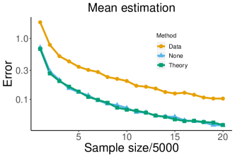
(a)

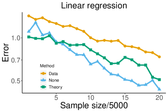
(b)

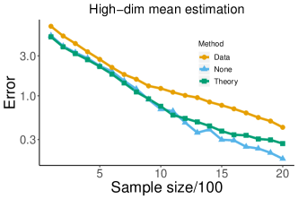
(c)

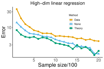
(d)

Figure 1: Average $\ell_{2}$-error over 100 repetitions plotted against sample size $n$, with privacy level set at (0.5, $10/n^{1.1}$). (a) & (b): mean estimation and linear regression with $d=20$ and $n$ from 5000 to 100000. (c) & (d): high-dimensional mean estimation and linear regression with $n$ increasing from 100 to 2000, $d=n$, and $s=20$.

5.2 Tuning of ${s}$

Our algorithms for high-dimensional problems require a sparsity tuning parameter $s$. We compare their performances when supplied with the true sparsity $s^{*}$ and when $s$ is chosen by 5-fold cross validation. The cross-validation error is first computed over a uniform grid of values from $s^{*}/2$ to $2s^{*}$. We then truncate these cross-validation errors with Algorithm $1^{\prime}$ in [32], so that the truncated cross-validation errors have bounded sensitivity. With bounded sensitivity, the exponential mechanism [35] can be applied to the (truncated) cross-validation errors to select a value of $s$ in a differentially private manner.

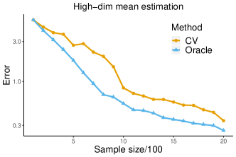
(a)

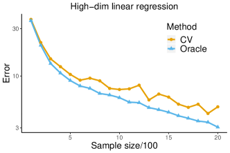
(b)

Figure 2: Average $\ell_{2}$-error over 50 repetitions plotted against sample size $n$, with privacy level set at (0.5, $10/n^{1.1}$). (a) & (b): high-dimensional mean estimation and linear regression with $n$ increasing from 100 to 2000, $d=n$, and $s=20$.

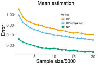
(a)

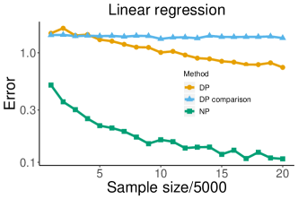
(b)

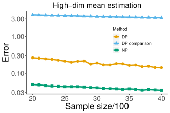
(c)

(d)

Figure 3: Average $\ell_{2}$-error over 100 repetitions plotted against sample size $n$, with privacy level set at (0.5, $10/n^{1.1}$). (a) & (b): mean estimation and linear regression with fixed $d=20$ and $n$ increasing from 5000 to 100000. (c) & (d): high-dimensional mean estimation and linear regression with $n$ increasing from 2000 to 4000, $d=2n$, and $s=20$.

Informed by the previous section on tuning $R$, the truncation tuning parameters for experiments in this section are selected by the data-driven method. In each problem, as the plots show, selecting $s$ by cross validation leads to errors comparable with their counterparts when the algorithms are supplied with the true sparsity $s^{*}$.

5.3 Comparisons with other algorithms

We compare our algorithms with their non-private counterparts, as well as other differentially private algorithms in the literature. For the low-dimensional problems, we consider Algorithm 4 in [29] for mean estimation and Algorithm 1 in [41] for regression. For the high-dimensional problems, we compare with the method in [45].

There are significant gaps in performance between our algorithms and those in [41, 45]. It is important to note, however, that the primary strength of Algorithm 1 in [41] is its ability to produce accurate test statistics with differential privacy, and the algorithm by [45] is primarily targeted at minimizing the excess empirical risk, so these numerical experiments may not be fully reflective of their advantages.

To further understand the improved numerical performance, we report here some observations from the numerical experiments. For the private Johnson-Lindenstrauss projection algorithm in [41], we observed that the ridge regression subroutine of the algorithm is frequently activated even when $n$ is very large, resulting in a ridge regression solution with regularization parameter of order $O(\log(1/\delta)/\varepsilon)$ and leading to significant bias. For the private Frank-Wolfe algorithm in [45], the solution is often non-sparse with large values outside the true support of ${\bm{\beta}}$, while our algorithm guarantees a sparse solution by construction and converges to the non-private solution as $n$ grows.

6 Data Analysis

In this section, we demonstrate the numerical performance of the differentially private algorithms on real data sets.

6.1 SNP array of adults with schizophrenia

We analyze the SNP array data of adults with schizophrenia, collected by [34], to illustrate the performance of our high-dimensional sparse mean estimator. In the dataset, there are 387 adults with schizophrenia, 241 of which are labeled as “average IQ” and 146 of which are labeled as “low IQ”. The SNP array is obtained by genotyping the subjects with the Affymetrix Genome-Wide Human SNP 6.0 platform. For our analysis, we focus on the 2000 SNPs with the highest minor allele frequencies (MAFs); the full dataset is available at https://www.ncbi.nlm.nih.gov/geo/query/acc.cgi?acc=GSE106818.

Privacy-perserving data analysis is very much relevant for this dataset and genetic data in general, because as [25] shows, an adversary can infer the absence/presence of an individual ’s genetic data in a large dataset by cross-referencing summary statistics, such as MAFs, from multiple genetic datasets. As MAFs can be calculated from the mean of an SNP array, differentially-private estimators of the mean allow reporting the MAFs without compromising any individual’s privacy.

The data set takes the form of a $387\times 2000$ matrix. The entries of the matrix take values 0, 1 or 2, representing the number of minor allele(s) at each SNP, and therefore the MAF of each SNP location in this sample can be obtained by computing the mean of the rows in this matrix. Sparsity is introduced by considering the difference in MAFs of the two IQ groups: the MAFs of the two groups are likely to differ at a small number of SNP locations among the 2000 SNPs considered.

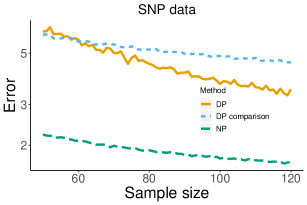
(a)

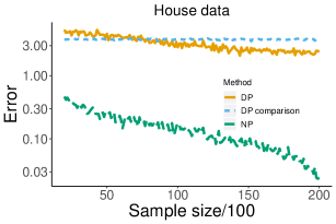
(b)

Figure 4: (a): The estimate of $\mathbb{E}[\|\hat{\bm{\mu}}-{\bm{\mu}}\|_{2}]$ for the differentially private sparse mean estimator as sample size increases from $50$ to $120$, with $s=20$.
(b): The estimate of $\mathbb{E}[\|\hat{\bm{\beta}}-{\bm{\beta}}\|_{2}]$ for the differentially private OLS estimator, compared with its differentially private counterpart, as sample size increases from $2000$ to $20000$.

For $m$ ranging from $10$ to $120$, we subsample $m$ subjects from each of the two IQ groups, say $\{\bm{x}_{11},\bm{x}_{12},\cdots\bm{x}_{1m}\}$ and $\{\bm{x}_{21},\bm{x}_{22},\cdots\bm{x}_{2m}\}$, and apply our sparse mean estimator to $\{\bm{x}_{11}-\bm{x}_{21},\bm{x}_{12}-\bm{x}_{22},\cdots\bm{x}_{1m}-\bm{x}_{2m}\}$ with $s=20$ and privacy parameters $(\varepsilon,\delta)=(0.5,10/n^{1.1})$. The error of this estimator is then calculated by comparing with the mean of the entire sample. This procedure is repeated 100 times to obtain Figure 4(a), which displays the estimate of $\mathbb{E}[\|\hat{\bm{\mu}}-{\bm{\mu}}\|_{2}]$ as $m$ increases from $50$ to $120$. We also plotted the corresponding curve for the method in [45] for comparison.

6.2 Housing prices in California

For the linear regression problem, we analyze a housing price dataset with economic and demographic covariates, constructed by [38] and available for download at http://lib.stat.cmu.edu/datasets/houses.zip. In this dataset, each subject is a block group in California in the 1990 Census; there are 20640 block groups in this dataset. The response variable is the median house value in the block group; the covariates include the median income, median age, total population, number of households, and the total number of rooms of all houses in the block group. In general, summary statistics such as mean or median do not have any differential privacy guarantees, so the absence of information on individual households in the dataset does not preclude an adversary from extracting sensitive individual information from the summary statistics. Privacy-preserving methods are still desirable in this case.

For $m$ ranging from $100$ to $20600$, we subsample $m$ subjects from the dataset to compute the differentially private OLS estimate, with privacy parameters $(\varepsilon,\delta)=(0.5,10/n^{1.1})$. The error of this estimator is then calculated by comparing with the non-private OLS estimator computed using the entire sample. This procedure is repeated 100 times to obtain Figure 4(b), which displays the estimate of $\mathbb{E}[\|\hat{\bm{\beta}}-{\bm{\beta}}\|_{2}]$ as $m$ increases from $2000$ to $20000$. The design matrix is standardized before applying the algorithm. The corresponding curve for the method in [41] is also plotted for comparison.

7 Discussion

Our paper investigates the tradeoff between statistical accuracy and privacy, by providing minimax lower bounds with differential privacy constraint and proposing differentially private algorithms with rates of convergence attaining the lower bounds up to logarithmic factors. For the lower bounds, we considered a technique based on tracing adversary and illustrated its utility by establishing minimax lower bounds for differentially private mean estimation and linear regression. These lower bounds are shown to be tight up to logarithmic factors via analysis of differentially private algorithms with matching rates of convergence.

Beyond the theoretical results, numerical performance of the private algorithms are demonstrated in simulations and real data analysis. The results suggest that the proposed algorithms have robust performance with respect to various choices of tuning parameters, achieve accuracy comparable to or better than that of existing differentially private algorithms, and can compute efficiently for sample sizes and dimensions up to tens of thousands. The numerical results corroborate the cost of privacy delineated in the theorems by exhibiting shrinking but non-vanishing gaps of accuracy between the private algorithms and their non-private counterparts. The theoretical and numerical results together can inform practitioners of differential privacy the necessary sacrifice of accuracy at a prescribed level of privacy, or the appropriate choice of privacy parameters if a given level of accuracy is desired.

There are many promising avenues for future research. It is of significant interest to study the optimal tradeoff of privacy and accuracy in statistical problems beyond mean estimation and linear regression. Examples include covariance/precision matrix estimation, graphical model recovery, non-parametric regression, and principal component analysis. Along the way, it is of importance to further develop general approaches of designing privacy-preserving algorithms, as well as more general lower bound techniques than those presented in this work.

One natural extension is uncertainty quantification with privacy constraints, which is largely unexplored in the statistics literature. Notably, [29] established the rate-optimal length of differentially private confidence intervals for the (one-dimensional) Gaussian mean. The technical tools developed in our paper may provide insights for constructing optimal statistical inference procedures in the context of, say, high-dimensional sparse mean estimation and linear regression.

Yet another intriguing direction of research is the cost of other notions of privacy, such as concentrated differential privacy [19], Rényi differential privacy [36], and Gaussian differential privacy [13]. These notions of privacy have found important applications such as stochastic gradient Langevin dynamics, stochastic Monte Carlo sampling [47] and deep learning [8].

8 Proofs

In this section, we prove the lower bound of low-dimensional mean estimation, Lemma 3.1 and Theorem 3.1, and the upper bound of high-dimensional linear regression, Theorem 4.4.

8.1 Proof of Lemma 3.1

Proof of Lemma 3.1.

Let $k=(C/2)\log(\frac{1}{n\delta})/\varepsilon$, with the value of $0<C<1$ to be chosen later. By the assumed regime of $\delta$ as a function of $n$, we have $k\asymp\log(1/\delta)/\varepsilon$ and $k<n/2$. We assume that $k$ divides $n$ without the loss of generality.

For an arbitrary $M\in\mathcal{M}_{\varepsilon,\delta}$, we define $M_{k}(\bm{Z})\equiv M(\bm{Y})$. Because $M$ is $(\varepsilon,\delta)$-differentially private, $M_{k}$ is also differentially private by post-processing. To lower bound $\mathbb{E}[\|M(\bm{Y})-\mathbb{E}\bm{y}_{1}\|_{2}|\bm{Z}]$, we observe that it suffices to find some appropriate distribution of $\bm{Z}$ so that $\mathbb{E}\|M_{k}(\bm{Z})-\bar{\bm{Z}}\|_{2}$ can be lower bounded: as $\|M(\bm{Y})-\mathbb{E}\bm{y}_{1}\|_{2}=\|M_{k}(\bm{Z})-\bar{\bm{Z}}\|_{2}$ by construction, there must be a realization of $\bm{Z}$ such that $\mathbb{E}[\|M(\bm{Y})-\mathbb{E}\bm{y}_{1}\|_{2}|\bm{Z}]$ is also lower bounded.

Since the sample size of $\bm{Z}$ does satisfy the assumption of the preliminary lower bound (2.3), the bound does apply provided that $M_{k}$ is a differentially private algorithm with respect to $\bm{Z}$. To this end, we consider the group privacy lemma:

Lemma 8.1 (group privacy, [43]).

For every $m\geq 1$, if $M$ is $(\varepsilon,\delta)$-differentially private, then for every pair of datasets $\bm{X}=\{\bm{x}_{k}\}_{k}$ and $\bm{Z}=\{\bm{z}_{k}\}_{k}$ satisfying $\sum_{i}\mathbbm{1}(\bm{x}_{i}\neq\bm{z}_{i})\leq m$, and every measurable set $S$,

$$\mathbb{P}(M(\bm{X})\in S)\leq e^{\varepsilon m}\mathbb{P}(M(\bm{Z})\in S)+\frac{e^{\varepsilon m}-1}{e-1}\cdot\delta.$$

The group privacy lemma suggests that, to characterize the privacy parameters of $M_{k}$, it suffices to upper-bound the number of changes in $\bm{Y}$ incurred by replacing one element of $\bm{Z}$. Let $m_{i}$ denote the number of times that $\bm{z}_{i}$ appears in a sample of size $n$ drawn with replacement from $\bm{Z}$, then our quantity of interest here is simply $\max_{i\in[n/k]}m_{i}$.

To analyze $\max_{i\in[n/k]}m_{i}$, we first show that $\delta$ as a function of $n$ must satisfy one of the following two statements.

1. There is a fixed constant $\tau$ such that $\frac{n}{(n/k)\log(n/k)}\leq{C\tau}/{\varepsilon}$ when $n$ is sufficiently large.

2. Case 1 fails to hold: we have $k>(C/2)\tau/\varepsilon\log(n/k)$ for any constant $\tau$, as long as $n$ is sufficiently large.

The dichotomy is made possible by the assumption that $\log(\delta)/\log(n)$ is non-increasing in $n$ and $\delta<n^{-(1+\omega)}$ for some fixed $\omega>0$. Under this assumption, we have either $\lim_{n\to\infty}\log(\delta)/\log(n)=c<-1$ or $\lim_{n\to\infty}\log(\delta)/\log(n)=-\infty$.

For the first case, we have $k=(C/2)\log(\frac{1}{n\delta})/\varepsilon=(C/2\varepsilon)\cdot(\log(1/\delta)-\log(n))\in((C/2\varepsilon)\cdot c_{1}\log n,(C/2\varepsilon)\cdot c_{2}\log n)$ for some $c_{1},c_{2}>0$ when $n$ is sufficiently large. Therefore

$$\frac{n}{(n/k)\log(n/k)}=\frac{k}{\log(n/k)}\leq\frac{c_{2}\cdot(C/2\varepsilon)\cdot\log n}{\log(2n\varepsilon/(C\cdot c_{1}\cdot\log n))}\leq{C\tau}/{\varepsilon},$$

for some $\tau>0$. This corresponds to the first statement.

For the second case $\lim_{n\to\infty}\log(\delta)/\log(n)=-\infty$, we then have for any constant $c_{3}>0$ and sufficiently large $n$, $\log(1/\delta)>c_{3}\log(n)$. Then $k=(C/2)\log(\frac{1}{n\delta})/\varepsilon=(C/2\varepsilon)\cdot(\log(1/\delta)-\log(n))\geq(C/2\varepsilon)\cdot(c_{3}-1)\log n$. Consequently we have

$$\frac{k}{\log(n/k)}>\frac{(c_{3}-1)\cdot(C/2\varepsilon)\cdot\log n}{\log(n)}\leq(c_{3}-1)\cdot(C/2\varepsilon)$$

for sufficiently large $n$. Since $c_{3}$ can take value of any positive number, this corresponds to the second statement.

Case 1. As $(m_{1},m_{2},\cdots,m_{n/k})$ follows a uniform multinomial distribution, we consider a useful result from [39], stated below:

Lemma 8.2 ([39]).

If $(y_{1},y_{2},\cdots,y_{d})$ follows a uniform multinomial$(\ell)$ distribution, and $\frac{\ell}{d\log d}\leq c$ for some constant $c$ not depending on $\ell$ and $d$, then for every $\zeta>0$,

$$\mathbb{P}\left(\max_{i\in[d]}y_{i}>(r_{c}+\zeta)\log d\right)=o(1),$$

where $r_{c}$ is the unique root of $1+y(\log c-\log y+1)-c=0$ that is strictly greater than $c$.

It follows that $\mathbb{P}\left(\max_{i}m_{i}\leq r\log n\right)=1-o(1)$, where $r$ is the unique root of $1+x(\log(C\tau/\varepsilon)-\log x+1)-(C\tau/\varepsilon)=0$ that is greater than $C\tau/\varepsilon$. Such a root exists, because $f_{C,\tau,\varepsilon}(x):=1+x(\log(C\tau/\varepsilon)-\log x+1)-(C\tau/\varepsilon)$ is strictly concave and achieves the global maximum value of $1$ at $x=C\tau/\varepsilon$.

Let $\mathcal{E}:=\{\max_{i}m_{i}\leq r\log n\}$. Under $\mathcal{E}$, Lemma 8.1 implies that $M_{k}$ is an $(\varepsilon r\log n,$ $\delta e^{\varepsilon r\log n})$-differentially private algorithm. We may essentially repeat the lower bound argument leading to the preliminary lower bound (2.3), as follows. Let $\bm{Z}=\{\bm{z}_{1},\bm{z}_{2},\cdots,\bm{z}_{n/k}\}$ be sampled i.i.d, from the data distribution specified in Lemma 2.1 including the prior distribution on ${\bm{\mu}}=\mathbb{E}z_{1}$, so that Lemma 2.1 applies to $\bm{Z}$. For every $i\in[n/k]$, let $\mathcal{C}=\{\sum_{i\in[n/k]}\mathcal{A}_{\bm{\mu}}(\bm{z}_{i},M_{k}(\bm{Z}))\leq(n/k)\sigma^{2}\sqrt{8d\log(1/\delta)}\}$. We have

$$\mathbb{P}(\|M_{k}(\bm{Z})-\bar{\bm{Z}}\|_{2}<c\sigma\sqrt{d})\leq\mathbb{P}(\mathcal{E}^{c})+\mathbb{P}\left(\mathcal{C}\cap\{\|M_{k}(\bm{Z})-\bar{\bm{Z}}\|_{2}<c\sigma\sqrt{d}\}\right)+\mathbb{P}(\mathcal{C}^{c})$$

$$\leq\mathbb{P}(\mathcal{E}^{c})+\mathbb{P}\left(\mathcal{C}\cap\{\|M_{k}(\bm{Z})-\bar{\bm{Z}}\|_{2}<c\sigma\sqrt{d}\}\right)+\sum_{i\in[n/k]}\mathbb{P}\left(\mathcal{A}_{\bm{\mu}}(\bm{z}_{i},M_{k}(\bm{Z}))>\sigma^{2}\sqrt{8d\log(1/\delta)}\right)$$

$$\leq o(1)+\delta+n(e^{\varepsilon r\log n}\delta+\delta e^{\varepsilon r\log n})=o(1)+\delta+2n^{-\tau+\varepsilon r}.$$

This probability is always bounded away from 1, because $\varepsilon r<\tau$ with appropriately chosen $C$: since $f_{C,\tau,\varepsilon}(\tau/\varepsilon)=(\tau/\varepsilon)(1+\log C-C)+1$ and $0<\varepsilon<1$, for every $\tau>0$ there is a sufficiently small $0<C<1$ such that $f_{C,\tau,\varepsilon}(\tau/\varepsilon)<0$. Since $f_{C,\tau,\varepsilon}(C\tau/\varepsilon)=1$ is the global maximum, we have $r<\tau/\varepsilon$, or equivalently $\varepsilon r<\tau$, as desired.

Case 2. each $m_{i}$ is a sum of $n$ independent Bernoulli$(k/n)$ random variables. Chernoff’s inequality implies that

$$\mathbb{P}\left(\max_{i}m_{i}>\frac{1}{\varepsilon}\log\left(\frac{1}{2n\delta}\right)\right)\leq\frac{n}{k}\cdot\exp\left(-\frac{(1/2C-1)}{3}k\right).$$

Recall that $k=(C/2)\log(\frac{1}{2n\delta})/\varepsilon$ by construction. By the assumption of Case 2, we have $k>(C/2)\tau/\varepsilon\log(n/k)$ for any constant $\tau$, as long as $n$ is sufficiently large. Then we have

$$\mathbb{P}\left(\max_{i}m_{i}>\frac{1}{\varepsilon}\log\left(\frac{1}{2n\delta}\right)\right)\leq\left(\frac{n}{k}\right)^{1-(1-C/2)\tau/3\varepsilon}.$$

The probability can be made arbitrarily small by fixing $C=1/2$ and choosing large $\tau$. Now that we have a high-probability bound for $\max_{i}m_{i}$, the group privacy lemma and union bound, as in Case 1, imply that $\mathbb{P}(\mathcal{C})=o(1)$, and therefore by Lemma 2.1

$$\mathbb{P}(\|M_{k}(\bm{Z})-\bar{\bm{Z}}\|_{2}<c\sigma\sqrt{d})$$

$$\leq \mathbb{P}(\mathcal{E}^{c})+\mathbb{P}\left(\mathcal{C}\cap\{\|M_{k}(\bm{Z})-\bar{\bm{Z}}\|_{2}<c\sigma\sqrt{d}\}\right)+\mathbb{P}(\mathcal{C}^{c})=o(1).$$

In each of the two cases, we found that $\mathbb{P}(\|M_{k}(\bm{Z})-\bar{\bm{Z}}\|_{2}<c\sigma\sqrt{d})=o(1)$. The proof is now complete by the reduction from $\mathbb{E}\left[\|M(\bm{Y})-\mathbb{E}\bm{y}_{1}\|_{2}|\bm{Z}\right]$ to $\mathbb{E}\|M_{k}(\bm{Z})-\bar{\bm{Z}}\|_{2}$. ∎

8.2 Proof of Theorem 3.1

It suffices to prove the second term of the minimax lower bound, as the first term is the statistical minimax lower bound for sub-Gaussian mean estimation.

For $i\in[n]$, consider $\bm{x}_{i}=\bm{0}\in{\mathbb{R}}^{d}$ with probability $1-\alpha$ and $\bm{x}_{i}=\bm{y}_{i}$ with probability $\alpha$, where $\bm{y}_{i}$ follows the discrete uniform distribution specified in Lemma 3.1. When $n\gtrsim\sqrt{d\log(1/\delta)}/\varepsilon$, there exists some $0<\alpha<1$ such that $\alpha n\asymp\sqrt{d\log(1/\delta)}/\varepsilon$. The distribution of $\bm{x}_{i}$ is indeed sub-Gaussian$(\sigma)$ with ${\bm{\mu}}\in\Theta$.

Consider the random index set $\mathcal{S}=\{i\in[n]:\bm{x}_{i}\neq\bm{0}\}$. For every $M\in\mathcal{M}_{\varepsilon,\delta}$, we have

$$\mathbb{E}[\|M(\bm{X})-{\bm{\mu}}\|_{2}]\geq\sum_{\mathcal{S}=S\subseteq[n],|S|\leq n\alpha}\mathbb{E}[\|M(\bm{X})-{\bm{\mu}}\|_{2}|\mathcal{S}=S]\mathbb{P}(\mathcal{S}=S).$$

Now for each fixed $S$, define $\tilde{M}(\bm{X}_{S})=\alpha^{-1}\mathbb{E}[M(\bm{X})|\mathcal{S}=S]$. We note that $\tilde{M}(\bm{X}_{S})$ is an $(\varepsilon,\delta)$-differentially private algorithm with respect to $\bm{X}_{S}$, by observing that $\mathbb{E}[M(\bm{X})|\mathcal{S}=S]=M(\{\bm{x}_{i}:i\in S\}\cup\{\bm{0}\}^{n-|S|})$ and therefore modifying any single datum in $\bm{X}_{S}=\{\bm{x}_{i}:i\in S\}$ incurs the same privacy loss to $M$ as it does to $\tilde{M}$. By construction, it also holds that ${\bm{\mu}}=\mathbb{E}\bm{x}_{1}=\alpha\mathbb{E}\bm{y}_{1}$. We then have

$$\mathbb{E}[\|M(\bm{X})-{\bm{\mu}}\|_{2}|\mathcal{S}=S] \geq\mathbb{E}[\|\alpha\tilde{M}(\bm{X}_{S})-\alpha\mathbb{E}\bm{y}_{1}\|_{2}|\mathcal{S}=S]$$

$$\geq\alpha\mathbb{E}[\|\tilde{M}(\bm{X}_{S})-\mathbb{E}\bm{y}_{1}\|_{2}]\gtrsim\alpha\sigma\sqrt{d}\asymp\sigma\frac{d\sqrt{\log(1/\delta)}}{n\varepsilon}.$$

For the last inequality, we invoked the lower bound proved in Lemma 3.1, since the sample size of $\bm{Y}$ is $\alpha n\asymp\sqrt{d\log(1/\delta)}/\varepsilon$. The proof is complete.

8.3 Proof of Theorem 4.4

Proof of Theorem 4.4.

Let $\hat{\bm{\beta}}=\operatorname*{arg\,min}_{\|{\bm{\beta}}\|_{2}\leq c_{0},\|{\bm{\beta}}\|_{0}\leq s^{*}}{\mathcal{L}}_{n}({\bm{\beta}})$. While global strong convexity and smoothness are no longer possible when $d>n$, because ${\bm{\beta}}^{t}$ and $\hat{\bm{\beta}}$ are sparse, we have following fact known as restricted strong convexity (RSC) and restricted smoothness (RSM) [37, 3, 33].

Fact 8.1.

Under assumptions of Theorem 4.4, it holds with probability at least $1-c_{1}\exp(-c_{2}n)$ that

$$\frac{1}{8Ls}\|{\bm{\beta}}^{t}-\hat{\bm{\beta}}\|_{2}^{2}\leq\langle\nabla{\mathcal{L}}_{n}({\bm{\beta}}^{t})-\nabla{\mathcal{L}}_{n}(\hat{\bm{\beta}}),{\bm{\beta}}^{t}-\hat{\bm{\beta}}\rangle\leq\frac{4L}{s}\|{\bm{\beta}}^{t}-\hat{\bm{\beta}}\|_{2}^{2}.$$ (8.1)

Under the event $\mathcal{E}_{1}=\left\{\Pi_{R}(y_{i})=y_{i},\forall i\in[n]\right\}$, Fact 8.1 implies that ${\mathcal{L}}_{n}({\bm{\beta}}^{t})-{\mathcal{L}}_{n}(\hat{\bm{\beta}})$ decays exponentially fast in $t$.

Lemma 8.3.

Under assumptions of Theorem 4.4 and event $\mathcal{E}_{1}$, $\eqref{eq: rsc and rsm}$ implies that there exists an absolute constant $\rho$ such that

$${\mathcal{L}}_{n}({\bm{\beta}}^{t+1})-{\mathcal{L}}_{n}(\hat{\bm{\beta}})\leq\left(1-\frac{1}{\rho L^{2}}\right)\left({\mathcal{L}}_{n}({\bm{\beta}}^{t})-{\mathcal{L}}_{n}(\hat{\bm{\beta}})\right)+c_{3}\left(\sum_{i\in[s]}\|\bm{w}^{t}_{i}\|_{\infty}^{2}+\|\tilde{\bm{w}}^{t}_{S^{t+1}}\|_{2}^{2}\right),$$ (8.2)

for every $t$, where $\bm{w}^{t}_{1},\bm{w}^{t}_{2},\cdots,\bm{w}^{t}_{s}$ are the Laplace noise vectors added to ${\bm{\beta}}^{t}-(\eta^{0}/n)\sum_{i=1}^{n}(\bm{x}_{i}^{\top}{\bm{\beta}}^{t}-\Pi_{R}(y_{i}))\bm{x}_{i}$ when the support of ${\bm{\beta}}^{t+1}$ is iteratively selected by “Peeling”, $S^{t+1}$ is the support of ${\bm{\beta}}^{t+1}$, and $\tilde{\bm{w}}^{t}$ is the noise vector added to the selected $s$-sparse vector.

We take Lemma 8.3, which is proved in Section A.7 of the supplement [10], to prove Theorem 4.4. We iterate (8.2) over $t$ and notate $\bm{W}_{t}=c_{3}\left(\sum_{i\in[s]}\|\bm{w}^{t}_{i}\|^{2}_{\infty}+\|\tilde{\bm{w}}^{t}_{S^{t+1}}\|_{2}^{2}\right)$ to obtain

$${\mathcal{L}}_{n}({\bm{\beta}}^{T})-{\mathcal{L}}_{n}(\hat{\bm{\beta}}) \leq\left(1-\frac{1}{\rho L^{2}}\right)^{T}\left({\mathcal{L}}_{n}({\bm{\beta}}^{0})-{\mathcal{L}}_{n}(\hat{\bm{\beta}})\right)+\sum_{k=0}^{T-1}\left(1-\frac{1}{\rho L^{2}}\right)^{T-k-1}\bm{W}_{k}$$

$$\leq\left(1-\frac{1}{\rho L^{2}}\right)^{T}8Lc_{0}^{2}+\sum_{k=0}^{T-1}\left(1-\frac{1}{\rho L^{2}}\right)^{T-k-1}\bm{W}_{k}.$$ (8.3)

The second inequality is a consequence of the upper inequality in (8.1) and the $\ell_{2}$ bounds of ${\bm{\beta}}^{0}$ and $\hat{\bm{\beta}}$. We can also bound ${\mathcal{L}}_{n}({\bm{\beta}}^{T})-{\mathcal{L}}_{n}(\hat{\bm{\beta}})$ from below by the lower inequality in (8.1):

$${\mathcal{L}}_{n}({\bm{\beta}}^{T})-{\mathcal{L}}_{n}(\hat{\bm{\beta}})\geq{\mathcal{L}}_{n}({\bm{\beta}}^{T})-{\mathcal{L}}_{n}({\bm{\beta}}^{*})\geq\frac{1}{16Ls}\|{\bm{\beta}}^{T}-{\bm{\beta}}^{*}\|_{2}^{2}-\langle\nabla{\mathcal{L}}_{n}({\bm{\beta}}^{*}),{\bm{\beta}}^{*}-{\bm{\beta}}^{T}\rangle.$$ (8.4)

Now (8.3) and (8.4) imply that, with $T=(\rho L^{2})\log(8c_{0}^{2}Ln)$,

$$\frac{1}{16Ls}\|{\bm{\beta}}^{T}-{\bm{\beta}}^{*}\|_{2}^{2}\leq\|\nabla{\mathcal{L}}_{n}({\bm{\beta}}^{*})\|_{\infty}\sqrt{s+s^{*}}\|{\bm{\beta}}^{*}-{\bm{\beta}}^{T}\|_{2}+\frac{1}{n}+\sum_{k=0}^{T-1}\left(1-\frac{1}{\rho L^{2}}\right)^{T-k-1}\bm{W}_{k}.$$ (8.5)

To further bound $\|{\bm{\beta}}^{T}-{\bm{\beta}}^{*}\|_{2}^{2}$, we observe that under $\mathcal{E}_{1}$ and two other events

$$\mathcal{E}_{2}=\left\{\max_{t}\bm{W}_{t}\leq K\frac{R^{2}(s^{*})^{3}\log^{2}d\log(1/\delta)\log^{2}n}{n^{2}\varepsilon^{2}}\right\},$$

$$\mathcal{E}_{3}=\left\{\|\nabla{\mathcal{L}}_{n}({\bm{\beta}}^{*})\|_{\infty}\leq 4\sigma\|\bm{x}\|_{\infty}\sqrt{\frac{\log d}{n}}\right\},$$

(8.5) and assumptions (D1’), (D2’) yield

$$\|{\bm{\beta}}^{T}-{\bm{\beta}}\|^{2}_{\Sigma_{\bm{x}}}\lesssim\sigma^{2}\left(\frac{s^{*}\log d}{n}+\frac{(s^{*}\log d)^{2}\log(1/\delta)\log^{3}n}{n^{2}\varepsilon^{2}}\right).$$

It remains to show that the events $\mathcal{E}_{1},\mathcal{E}_{2},\mathcal{E}_{3}$ occur simultaneously with high probability. We have $\mathbb{P}(\mathcal{E}_{1}^{c})\leq c_{1}\exp(-c_{2}\log n)$ because $y_{1},y_{2},\cdots,y_{n}\stackrel{{\scriptstyle\text{i.i.d.}}}{{\sim}}N(0,\sigma^{2})$ and $R\asymp\sigma\sqrt{\log n}$.

For $\mathcal{E}_{2}$, we invoke Lemma A.1 in the supplement [10]. For each iterate $t$, the individual coordinates of $\tilde{\bm{w}}^{t}$, $\bm{w}^{t}_{i}$ are sampled i.i.d. from the Laplace distribution with scale $\eta^{0}\cdot\frac{2B\sqrt{3s\log(T/\delta)}}{n\varepsilon/T}$, where the noise scale $B\lesssim R/\sqrt{s}$ and $T\asymp\log n$ by our choice. If $n\geq K\cdot\left(R(s^{*})^{3/2}\log d\sqrt{\log(1/\delta)}\log n/\varepsilon\right)$ for a sufficiently large constant $K$, Lemma A.1 and the union bound imply that, with probability at least $1-c_{1}\exp(-c_{2}\log(d/(s^{*}\log n))$, $\max_{t}\bm{W}_{t}$ is bounded by $K\frac{R^{2}(s^{*})^{3}\log^{2}d\log(1/\delta)\log^{2}n}{n^{2}\varepsilon^{2}}$ for some appropriate constant $K$. For $\mathcal{E}_{3}$, under assumptions (D1’) and (D2’), it is a standard probabilistic result (see, for example, [46] pp. 210-211) that $\mathbb{P}(\mathcal{E}^{c}_{3})\leq 2e^{-2\log d}$. ∎

Appendix A Proofs of upper bound results

A.1 Proof of Theorem 3.2

Proof of Theorem 3.2.

By the choice of $R$ and $\|{\bm{\mu}}\|_{\infty}\leq c=O(1)$, we have

$$\|\hat{\bm{\mu}}-{\bm{\mu}}\|_{2}^{2}\leq 2\|\bm{w}\|_{2}^{2}+2\|\overline{\bm{X}}-{\bm{\mu}}\|_{2}^{2}.$$

Once we take expectation, the conclusion follows from the distribution of $\bm{w}$ and the sub-Gaussianity of $\bm{x}$. ∎

A.2 Proof of Lemma 3.4

Proof of Lemma 3.4.

Let $\psi:R_{2}\to R_{1}$ be a bijection. By the selection criterion of Algorithm 3.2, for each $j\in R_{2}$ we have $|v_{j}|+w_{ij}\leq|v_{\psi(j)}|+w_{i\psi(j)}$, where $i$ is the index of the iteration in which $\psi(j)$ is appended to $S$. It follows that, for every $c>0$,

$$v_{j}^{2} \leq\left(|v_{\psi(j)}|+w_{i\psi(j)}-w_{ij}\right)^{2}$$

$$\leq(1+1/c)v_{\psi(j)}^{2}+(1+c)(w_{i\psi(j)}-w_{ij})^{2}\leq(1+1/c)v_{\psi(j)}^{2}+4(1+c)\|\bm{w}_{i}\|_{\infty}^{2}$$

Summing over $j$ then leads to

$$\|\bm{v}_{R_{2}}\|_{2}^{2}\leq(1+1/c)\|\bm{v}_{R_{1}}\|_{2}^{2}+4(1+c)\sum_{i\in[s]}\|\bm{w}_{i}\|^{2}_{\infty}.$$

∎

A.3 Proof of Theorem 3.4

Proof of Theorem 3.4.

Let $S,S^{*}$ denote the supports of $\hat{\bm{\mu}}$ and ${\bm{\mu}}$ respectively. By the choice of $R=K\sigma\sqrt{\log n}$ and $\|{\bm{\mu}}\|_{\infty}\leq c=O(1)$, we have

$$\|\hat{\bm{\mu}}-{\bm{\mu}}\|_{2}^{2}\leq 2\|\tilde{\bm{w}}_{S}\|_{2}^{2}+2\|(\overline{\bm{X}}-{\bm{\mu}})_{S\cap S^{*}}\|_{2}^{2}+\|\overline{\bm{X}}_{S\cap(S^{*})^{c}}-{\bm{\mu}}_{S^{*}\cap S^{c}}\|_{2}^{2}$$ (A.1)

For the last term,

$$\|\overline{\bm{X}}_{S\cap(S^{*})^{c}}-{\bm{\mu}}_{S^{*}\cap S^{c}}\|_{2}^{2} =\|\overline{\bm{X}}_{S\cap(S^{*})^{c}}-\overline{\bm{X}}_{S^{*}\cap S^{c}}+\overline{\bm{X}}_{S^{*}\cap S^{c}}-{\bm{\mu}}_{S^{*}\cap S^{c}}\|_{2}^{2}$$

$$\leq 4\|\overline{\bm{X}}_{S\cap(S^{*})^{c}}\|_{2}+4\|\overline{\bm{X}}_{S^{*}\cap S^{c}}\|+2\|(\overline{\bm{X}}-{\bm{\mu}})_{S^{*}\cap S^{c}}\|_{2}^{2}.$$ (A.2)

Since $s^{*}=|S^{*}|\leq|S|=s$ by assumption, we invoke Lemma 3.4 to obtain that

$$\|\overline{\bm{X}}_{S^{*}\cap S^{c}}\|\leq 2\|\overline{\bm{X}}_{S\cap(S^{*})^{c}}\|_{2}+8\sum_{i\in[s]}\|\bm{w}_{i}\|^{2}_{\infty}.$$ (A.3)

Now combining (A.3) with (A.3) and further with (A.1) yields

$$\|\hat{\bm{\mu}}-{\bm{\mu}}\|_{2}^{2}\leq 2\|(\overline{\bm{X}}-{\bm{\mu}})_{S^{*}}\|_{2}^{2}+12\|\overline{\bm{X}}_{S\cap(S^{*})^{c}}\|_{2}+32\sum_{i\in[s]}\|\bm{w}_{i}\|^{2}_{\infty}+2\|\tilde{\bm{w}}_{S}\|_{2}^{2}.$$ (A.4)

For the first two terms, since $|S|=s\asymp s^{*}$, we have

$$2\|(\overline{\bm{X}}-{\bm{\mu}})_{S^{*}}\|_{2}^{2}+12\|\overline{\bm{X}}_{S\cap(S^{*})^{c}}\|_{2}\lesssim s^{*}\|\overline{\bm{X}}-{\bm{\mu}}\|^{2}_{\infty}.$$

$\overline{\bm{X}}-{\bm{\mu}}$ is a zero-mean sub-Gaussian$(\sigma/\sqrt{n})$ random vector. Standard tail bounds for sub-Gaussian maxima (see, for example, [46]) implies that $\|\overline{\bm{X}}-{\bm{\mu}}\|^{2}_{\infty}<C\sigma^{2}\log d/n$ with probability at least $1-c_{1}\exp(-c_{2}\log n)$.

For the last two terms of (A.4), we have the following lemma.

Lemma A.1.

Consider $\bm{w}\in{\mathbb{R}}^{k}$ with $w_{1},w_{2},\cdots,w_{k}\stackrel{{\scriptstyle\text{i.i.d.}}}{{\sim}}$ Laplace$(\lambda)$. For every $C>1$,

$$\mathbb{P}\left(\|\bm{w}\|_{2}^{2}>kC^{2}\lambda^{2}\right)\leq ke^{-C}$$

$$\mathbb{P}\left(\|\bm{w}\|_{\infty}^{2}>C^{2}\lambda^{2}\log^{2}k\right)\leq e^{-(C-1)\log k}.$$

The lemma is proved in Section A.3.1. In our case, $\lambda=4R\sqrt{3s\log(1/\delta)}/n\varepsilon$ and $k=d$. It follows that

$$32\sum_{i\in[s]}\|\bm{w}_{i}\|^{2}_{\infty}+2\|\tilde{\bm{w}}_{S}\|_{2}^{2}\lesssim\sigma^{2}\frac{(s^{*}\log d)^{2}\log(1/\delta)\log n}{n^{2}\varepsilon^{2}}$$

with probability at least $1-c_{1}\exp(-c_{2}\log d)$. Combining the two high-probability bounds above completes the proof. ∎

A.3.1 Proof of Lemma A.1

Proof of Lemma A.1.

By union bound and the i.i.d. assumption,

$$\mathbb{P}\left(\|\bm{w}\|_{2}^{2}>kC^{2}\lambda^{2}\right)\leq k\mathbb{P}(w_{1}^{2}>C^{2}\lambda^{2})\leq ke^{-C}.$$

It follows that

$$\mathbb{P}\left(\|\bm{w}\|_{\infty}^{2}>C^{2}\lambda^{2}\log^{2}k\right)\leq k\mathbb{P}(w_{1}^{2}>C^{2}\lambda^{2}\log^{2}k)\leq ke^{-C\log k}=e^{-(C-1)\log k}.$$

∎

A.4 Proof of Lemma 4.2

Proof of Lemma 4.2.

As there are $T$ iterations in Algorithm 4.1, it suffices to show that each iteration is $(\varepsilon/T,\delta/T)$-differentially private, and then the overall privacy follows from the composition property of differential privacy.

Consider two data sets $\bm{Z}$ and $\bm{Z}^{\prime}$ that differ by one datum, $(y,\bm{x})\in\bm{Z}$ versus $(y^{\prime},\bm{x}^{\prime})\in\bm{Z}^{\prime}$. For each $t$, by (D1) and (P1), we control the $\ell_{2}$-sensitivity of the gradient step:

$$\frac{\eta^{0}}{n}\left(|\bm{x}^{\top}{\bm{\beta}}^{t}-\Pi_{R}(y)|\|\bm{x}\|_{2}+|(\bm{x}^{\prime})^{\top}{\bm{\beta}}^{t}-\Pi_{R}(y^{\prime})|\|\bm{x}^{\prime}\|_{2}\right)\leq\frac{\eta^{0}}{n}\cdot 4(R+c_{0}c_{\bm{x}})c_{\bm{x}}=\frac{\eta^{0}}{n}B.$$

By the Gaussian mechanism of differential privacy, it follows that ${\bm{\beta}}^{t+1}(\bm{Z})$ is an $(\varepsilon/T,\delta/T)$-differentially private algorithm, as desired. ∎

A.5 Proof of Theorem 4.2

Proof of Theorem 4.2.

Let $\bm{X}$ denote the $n\times d$ design matrix. We analyze the algorithm under the events

$$\mathcal{E}_{1}=\left\{d\|n^{-1}\bm{X}^{\top}\bm{X}-\Sigma_{\bm{x}}\|_{2}\leq 1/2L\right\}\text{ and }\mathcal{E}_{2}=\left\{\Pi_{R}(y_{i})=y_{i},\forall i\in[n]\right\},$$

and then show that they do occur with high probability.

Under $\mathcal{E}_{2}$, we have ${\bm{\beta}}^{t+1}=\Pi_{C}\left({\bm{\beta}}^{t}-\eta^{0}\nabla{\mathcal{L}}_{n}({\bm{\beta}}^{t})+\bm{w}_{t}\right)$. $\mathcal{E}_{1}$ and assumption (D2) imply that the objective function ${\mathcal{L}}_{n}$ is $(2L/d)$-smooth and $(1/2Ld)$-strongly convex. Let $\hat{\bm{\beta}}=\operatorname*{arg\,min}_{\|{\bm{\beta}}\|_{2}\leq C}{\mathcal{L}}_{n}$ and $\tilde{\bm{\beta}}^{t+1}={\bm{\beta}}^{t}-\eta^{0}\nabla{\mathcal{L}}_{n}({\bm{\beta}}^{t})$, it then follows that

$$\|{\bm{\beta}}^{t+1}-\hat{\bm{\beta}}\|_{2}^{2} \leq(1+1/8L^{2})\|\tilde{\bm{\beta}}^{t+1}-\hat{\bm{\beta}}\|_{2}^{2}+(1+8L^{2})\|\bm{w}_{t}\|_{2}^{2}$$

$$\leq(1+1/8L^{2})(1-1/4L^{2})\|{\bm{\beta}}^{t}-\hat{\bm{\beta}}\|_{2}^{2}+(1+8L^{2})\|\bm{w}_{t}\|_{2}^{2}$$

$$\leq(1-1/8L^{2})\|{\bm{\beta}}^{t}-\hat{\bm{\beta}}\|_{2}^{2}+(1+8L^{2})\|\bm{w}_{t}\|_{2}^{2}.$$ (A.5)

The second inequality holds by standard convergence analysis of gradient descent for $\gamma$-smooth and $\alpha$-strongly convex objective (see, for example, [nesterov2003introductory]): when the step size $\eta^{0}$ is chosen to be $1/\gamma$, it holds that $\|\tilde{\bm{\beta}}^{t+1}-\hat{\bm{\beta}}\|^{2}_{2}\leq(1-\alpha/\gamma)\|{\bm{\beta}}^{t}-\hat{\bm{\beta}}\|_{2}^{2}$.

Now by (A.5) and the choice of $C=c_{0}$, $T=(8L^{2})\log(c_{0}^{2}n)$, induction over $t$ gives

$$\|{\bm{\beta}}^{T}-\hat{\bm{\beta}}\|_{2}^{2} \leq\frac{1}{n}+\left(1+8L^{2}\right)\sum_{k=0}^{T-1}\left(1-1/8L^{2}\right)^{T-k-1}\|\bm{w}_{k}\|_{2}^{2}.$$ (A.6)

The noise term can be controlled by the following lemma:

Lemma A.2.

For $X_{1},X_{2},\cdots,X_{k}\stackrel{{\scriptstyle\text{i.i.d.}}}{{\sim}}\chi^{2}_{d}$, $\lambda>0$ and $0<\rho<1$,

$$\mathbb{P}\left(\sum_{j=1}^{k}\lambda\rho^{j}X_{j}>\frac{\rho\lambda d}{1-\rho}+\Delta\right)\leq\exp\left(-\min\left(\frac{(1-\rho^{2})\Delta^{2}}{8\rho^{2}\lambda^{2}d},\frac{\Delta}{8\rho\lambda}\right)\right).$$

The lemma is proved in Section A.5.1. To apply the tail bound, we let $\lambda=(\eta^{0})^{2}2B^{2}\frac{\log(2T/\delta)}{n^{2}(\varepsilon/T)^{2}}$ and $\Delta=K\lambda d$ for a sufficiently large constant $K$, then the noise term in (A.5) is bounded by $K\lambda d\asymp\sigma^{2}\frac{d^{3}\log(1/\delta)\log^{3}n}{n^{2}\varepsilon^{2}}$ with probability at least $1-c_{1}\exp(-c_{2}d)$. Now (A.5) combined with the statistical convergence rate of $\|\hat{\bm{\beta}}-{\bm{\beta}}\|_{2}^{2}$ and assumptions (D1), (D2) yields

$$\|{\bm{\beta}}^{T}-{\bm{\beta}}\|_{\Sigma_{\bm{x}}}^{2}\lesssim\sigma^{2}\left(\frac{d}{n}+\frac{d^{2}\log(1/\delta)\log^{3}n}{n^{2}\varepsilon^{2}}\right).$$

It remains to control the probability that either $\mathcal{E}_{1}$ or $\mathcal{E}_{2}$ fails to occur. For $\mathcal{E}_{1}$, standard matrix concentration bounds (see, for example, [vershynin2010introduction]), imply that there exists universal constant $c_{1},c_{2}$ such that, as long as $d<n$, $\mathbb{P}(\mathcal{E}_{1}^{c})\leq c_{1}\exp(-c_{2}n)$. Finally we have $\mathbb{P}(\mathcal{E}_{2}^{c})\leq c_{1}\exp(-c_{2}\log n)$ because $y_{1},y_{2},\cdots,y_{n}\stackrel{{\scriptstyle\text{i.i.d.}}}{{\sim}}N(0,\sigma^{2})$ and $R\asymp\sigma\sqrt{\log n}$. ∎

A.5.1 Proof of Lemma A.2

Proof of Lemma A.2.

Since $\mathbb{E}\sum_{j=1}^{k}\lambda\rho^{j}X_{j}\leq\lambda d\sum_{j=1}^{k}\rho^{j}<\frac{\rho\lambda d}{1-\rho}$, we have

$$\mathbb{P}\left(\sum_{j=1}^{k}\lambda\rho^{j}X_{j}>\frac{\rho\lambda d}{1-\rho}+t\right)\leq\mathbb{P}\left(\sum_{j=1}^{k}\lambda\rho^{j}(X_{j}-\mathbb{E}X_{j})>t\right).$$

The (centered) $\chi^{2}_{d}$ random variable is sub-exponential with parameters $(2\sqrt{d},4)$, the weighted sum is also sub-exponential, with parameters at most $\left(2\lambda\sqrt{d}\sqrt{\sum_{j=1}^{k}\rho^{2j}},4\lambda\rho\right)$. The desired tail bound now follows directly from standard sub-exponential tail bounds. ∎

A.6 Proof of Lemma 4.4

Proof of Lemma 4.4.

As there are $T$ iterations in Algorithm 4.2, it suffices to show that each iteration is $(\varepsilon/T,\delta/T)$-differentially private, and then the overall privacy follows from the composition property of differential privacy.

Consider two data sets $\bm{Z}$ and $\bm{Z}^{\prime}$ that differ by one datum, $(y,\bm{x})\in\bm{Z}$ versus $(y^{\prime},\bm{x}^{\prime})\in\bm{Z}^{\prime}$. For each $t$, by (D1’) and (P1’), we have

$$\frac{\eta^{0}}{n}\left(|\bm{x}^{\top}{\bm{\beta}}^{t}-\Pi_{R}(y)|\|\bm{x}\|_{\infty}+|(\bm{x}^{\prime})^{\top}{\bm{\beta}}^{t}-\Pi_{R}(y^{\prime})|\|\bm{x}^{\prime}\|_{\infty}\right)\leq\frac{\eta^{0}}{n}\cdot 4(R+c_{0}c_{\bm{x}})c_{\bm{x}}/\sqrt{s}=\frac{\eta^{0}}{n}B.$$

Lemma 3.3 then implies that each iteration of Algorithm 4.2 is $(\varepsilon/T,\delta/T)$-differentially private, as desired. ∎

A.7 Proof of Lemma 8.3

Proof of Lemma 8.3.

We begin with stating a key property of the “Peeling” algorithm (Algorithm 3.2).

Lemma A.3.

Let $\tilde{P}_{s}$ be defined as in Algorithm 3.2. For any index set $I$, any $\bm{v}\in{\mathbb{R}}^{I}$ and $\hat{\bm{v}}$ such that $\|\hat{\bm{v}}\|_{0}\leq\hat{s}\leq s$, we have that for every $c>0$,

$$\|\tilde{P}_{s}(\bm{v})-\bm{v}\|_{2}^{2}\leq(1+1/c)\frac{|I|-s}{|I|-\hat{s}}\|\hat{\bm{v}}-\bm{v}\|_{2}^{2}+4(1+c)\sum_{i\in[s]}\|\bm{w}_{i}\|^{2}_{\infty}.$$

The lemma is proved in Section A.7.1. We also introduce some notation for the proof.

• Let $\alpha=1/8Ls$ and $\gamma=4L/s$ so that (8.1) can be equivalently written as

  $$\alpha\|{\bm{\beta}}^{t}-\hat{\bm{\beta}}\|_{2}^{2}\leq\langle\nabla{\mathcal{L}}_{n}({\bm{\beta}}^{t})-\nabla{\mathcal{L}}_{n}(\hat{\bm{\beta}}),{\bm{\beta}}^{t}-\hat{\bm{\beta}}\rangle\leq\gamma\|{\bm{\beta}}^{t}-\hat{\bm{\beta}}\|_{2}^{2}.$$ (A.7)

  Throughout the proof, we assume the truth of (A.7) to prove (8.2).

• Let $S^{t}={\rm supp}({\bm{\beta}}^{t})$, $S^{t+1}={\rm supp}({\bm{\beta}}^{t+1})$, $S^{*}={\rm supp}(\hat{\bm{\beta}})$, and define $I^{t}=S^{t+1}\cup S^{t}\cup S^{*}$.

• Let $\bm{g}^{t}=\nabla{\mathcal{L}}_{n}({\bm{\beta}}^{t})$ and $\eta^{0}=\eta/\gamma$, where $\gamma$ is the constant in (A.7).

• Let $\bm{w}_{1},\bm{w}_{2},\cdots,\bm{w}_{s}$ be the noise vectors added to ${\bm{\beta}}^{t}-\eta^{0}\nabla{\mathcal{L}}_{n}({\bm{\beta}}^{t})$ when the support of ${\bm{\beta}}^{t+1}$ is iteratively selected. We define $\bm{W}=4\sum_{i\in[s]}\|\bm{w}_{i}\|^{2}_{\infty}$.

By (A.7), we have

$${\mathcal{L}}_{n}({\bm{\beta}}^{t+1})-{\mathcal{L}}_{n}({\bm{\beta}}^{t}) \leq\langle{\bm{\beta}}^{t+1}-{\bm{\beta}}^{t},\bm{g}^{t}\rangle+\frac{\gamma}{2}\|{\bm{\beta}}^{t+1}-{\bm{\beta}}^{t}\|_{2}^{2}$$

$$=\frac{\gamma}{2}\left\|{\bm{\beta}}^{t+1}_{I^{t}}-{\bm{\beta}}^{t}_{I^{t}}+\frac{\eta}{\gamma}\bm{g}^{t}_{I^{t}}\right\|_{2}^{2}-\frac{\eta^{2}}{2\gamma}\left\|\bm{g}^{t}_{I^{t}}\right\|_{2}^{2}+(1-\eta)\langle{\bm{\beta}}^{t+1}-{\bm{\beta}}^{t},\bm{g}^{t}\rangle.$$ (A.8)

We first focus on the third term above. In what follows, $c$ denotes an arbitrary constant greater than 1. Since ${\bm{\beta}}^{t+1}$ is an output from Algorithm 3.2, we may write ${\bm{\beta}}^{t+1}={\tilde{\bm{\beta}}}^{t+1}+\tilde{\bm{w}}_{S^{t+1}}$, so that ${\tilde{\bm{\beta}}}^{t+1}=\tilde{P}_{s}({\bm{\beta}}^{t}-\eta^{0}\nabla{\mathcal{L}}_{n}({\bm{\beta}}^{t}))$ and $\tilde{\bm{w}}$ is a vector consisting of $d$ i.i.d. Laplace random variables.

$$\langle{\bm{\beta}}^{t+1}-{\bm{\beta}}^{t},\bm{g}^{t}\rangle =\langle{\bm{\beta}}^{t+1}_{S^{t+1}}-{\bm{\beta}}^{t}_{S^{t+1}},\bm{g}^{t}_{S^{t+1}}\rangle-\langle{\bm{\beta}}^{t}_{S^{t}\setminus S^{t+1}},\bm{g}^{t}_{S^{t}\setminus S^{t+1}}\rangle$$

$$=\langle{\tilde{\bm{\beta}}}^{t+1}_{S^{t+1}}-{\bm{\beta}}^{t}_{S^{t+1}},\bm{g}^{t}_{S^{t+1}}\rangle+\langle\tilde{\bm{w}}_{S^{t+1}},\bm{g}^{t}_{S^{t+1}}\rangle-\langle{\bm{\beta}}^{t}_{S^{t}\setminus S^{t+1}},\bm{g}^{t}_{S^{t}\setminus S^{t+1}}\rangle.$$

It follows that, for every $c>1$,

$$\langle{\bm{\beta}}^{t+1}-{\bm{\beta}}^{t},\bm{g}^{t}\rangle \leq-\frac{\eta}{\gamma}\|\bm{g}^{t}_{S^{t+1}}\|_{2}^{2}+c\|\tilde{\bm{w}}_{S^{t+1}}\|_{2}^{2}+(1/4c)\|\bm{g}^{t}_{S^{t+1}}\|_{2}^{2}-\langle{\bm{\beta}}^{t}_{S^{t}\setminus S^{t+1}},\bm{g}^{t}_{S^{t}\setminus S^{t+1}}\rangle.$$ (A.9)

Now for the last term in the display above, we have

$$-\langle{\bm{\beta}}^{t}_{S^{t}\setminus S^{t+1}},\bm{g}^{t}_{S^{t}\setminus S^{t+1}}\rangle \leq\frac{\gamma}{2\eta}\left(\left\|{\bm{\beta}}^{t}_{S^{t}\setminus S^{t+1}}-\frac{\eta}{\gamma}\bm{g}^{t}_{S^{t}\setminus S^{t+1}}\right\|_{2}^{2}-\left(\frac{\eta}{\gamma}\right)^{2}\|\bm{g}^{t}_{S^{t}\setminus S^{t+1}}\|_{2}^{2}\right)$$

$$\leq\frac{\gamma}{2\eta}\left\|{\bm{\beta}}^{t}_{S^{t}\setminus S^{t+1}}-\frac{\eta}{\gamma}\bm{g}^{t}_{S^{t}\setminus S^{t+1}}\right\|_{2}^{2}-\frac{\eta}{2\gamma}\|\bm{g}^{t}_{S^{t}\setminus S^{t+1}}\|_{2}^{2}.$$

We apply Lemma 3.4 to $\left\|{\bm{\beta}}^{t}_{S^{t}\setminus S^{t+1}}-\frac{\eta}{\gamma}\bm{g}^{t}_{S^{t}\setminus S^{t+1}}\right\|_{2}^{2}$ to obtain that, for every $c>1$,

$$-\langle{\bm{\beta}}^{t}_{S^{t}\setminus S^{t+1}},\bm{g}^{t}_{S^{t}\setminus S^{t+1}}\rangle \leq\frac{\gamma}{2\eta}\left[(1+1/c)\left\|\tilde{{\bm{\beta}}}^{t+1}_{S^{t+1}\setminus S^{t}}\right\|_{2}^{2}+(1+c)\bm{W}\right]-\frac{\eta}{2\gamma}\|\bm{g}^{t}_{S^{t}\setminus S^{t+1}}\|_{2}^{2}$$

$$=\frac{\eta}{2\gamma}\left[(1+1/c)\left\|\bm{g}^{t}_{S^{t+1}\setminus S^{t}}\right\|_{2}^{2}+(1+c)\frac{\gamma}{2\eta}\bm{W}\right]-\frac{\eta}{2\gamma}\|\bm{g}^{t}_{S^{t}\setminus S^{t+1}}\|_{2}^{2}.$$

Plugging the inequality above back into (A.9) yields

$$\langle{\bm{\beta}}^{t+1}-{\bm{\beta}}^{t},\bm{g}^{t}\rangle\leq~{} -\frac{\eta}{\gamma}\|\bm{g}^{t}_{S^{t+1}}\|_{2}^{2}+c\|\tilde{\bm{w}}_{S^{t+1}}\|_{2}^{2}+(1/4c)\|\bm{g}^{t}_{S^{t+1}}\|_{2}^{2}$$

$$+\frac{\eta}{2\gamma}\left[(1+1/c)\left\|\bm{g}^{t}_{S^{t+1}\setminus S^{t}}\right\|_{2}^{2}+(1+c)\frac{\gamma}{2\eta}\bm{W}\right]-\frac{\eta}{2\gamma}\|\bm{g}^{t}_{S^{t}\setminus S^{t+1}}\|_{2}^{2}$$

$$\leq~{} \frac{\eta}{2\gamma}\left\|\bm{g}^{t}_{S^{t+1}\setminus S^{t}}\right\|_{2}^{2}-\frac{\eta}{2\gamma}\|\bm{g}^{t}_{S^{t}\setminus S^{t+1}}\|_{2}^{2}-\frac{\eta}{\gamma}\|\bm{g}^{t}_{S^{t+1}}\|_{2}^{2}$$

$$+(1/c)\left(4+\frac{\eta}{2\gamma}\right)\|\bm{g}^{t}_{S^{t+1}}\|_{2}^{2}+c\|\tilde{\bm{w}}_{S^{t+1}}\|_{2}^{2}+(1+c)\frac{\gamma}{2\eta}\bm{W}.$$

Finally, for the third term of (A.8) we have

$$\langle{\bm{\beta}}^{t+1}-{\bm{\beta}}^{t},\bm{g}^{t}\rangle\leq-\frac{\eta}{2\gamma}\left\|\bm{g}^{t}_{S^{t}\cup S^{t+1}}\right\|_{2}^{2}+(1/c)\left(4+\frac{\eta}{2\gamma}\right)\|\bm{g}^{t}_{S^{t+1}}\|_{2}^{2}+c\|\tilde{\bm{w}}_{S^{t+1}}\|_{2}^{2}+(1+c)\frac{\gamma}{2\eta}\bm{W}.$$

Now combining this bound with (A.8) yields

$${\mathcal{L}}_{n}({\bm{\beta}}^{t+1})-{\mathcal{L}}_{n}({\bm{\beta}}^{t})$$

$$\leq~{} \frac{\gamma}{2}\left\|{\bm{\beta}}^{t+1}_{I^{t}}-{\bm{\beta}}^{t}_{I^{t}}+\frac{\eta}{\gamma}\bm{g}^{t}_{I^{t}}\right\|_{2}^{2}-\frac{\eta^{2}}{2\gamma}\left\|\bm{g}^{t}_{I^{t}}\right\|_{2}^{2}-\frac{\eta(1-\eta)}{2\gamma}\left\|\bm{g}^{t}_{S^{t}\cup S^{t+1}}\right\|_{2}^{2}$$

$$+\frac{1-\eta}{c}\left(4+\frac{\eta}{2\gamma}\right)\|\bm{g}^{t}_{S^{t+1}}\|_{2}^{2}+(1-\eta)c\|\tilde{\bm{w}}_{S^{t+1}}\|_{2}^{2}+(1-\eta)(1+c)\frac{\gamma}{2\eta}\bm{W}$$

$$\leq~{} \frac{\gamma}{2}\left\|{\bm{\beta}}^{t+1}_{I^{t}}-{\bm{\beta}}^{t}_{I^{t}}+\frac{\eta}{\gamma}\bm{g}^{t}_{I^{t}}\right\|_{2}^{2}-\frac{\eta^{2}}{2\gamma}\left\|\bm{g}^{t}_{I^{t}\setminus(S^{t}\cup S^{*})}\right\|_{2}^{2}-\frac{\eta^{2}}{2\gamma}\left\|\bm{g}^{t}_{S^{t}\cup S^{*}}\right\|_{2}^{2}-\frac{\eta(1-\eta)}{2\gamma}\left\|\bm{g}^{t}_{S^{t}\cup S^{t+1}}\right\|_{2}^{2}$$

$$+\frac{1-\eta}{c}\left(4+\frac{\eta}{2\gamma}\right)\|\bm{g}^{t}_{S^{t+1}}\|_{2}^{2}+(1-\eta)c\|\tilde{\bm{w}}_{S^{t+1}}\|_{2}^{2}+(1-\eta)(1+c)\frac{\gamma}{2\eta}\bm{W}$$

$$\leq~{} \frac{\gamma}{2}\left\|{\bm{\beta}}^{t+1}_{I^{t}}-{\bm{\beta}}^{t}_{I^{t}}+\frac{\eta}{\gamma}\bm{g}^{t}_{I^{t}}\right\|_{2}^{2}-\frac{\eta^{2}}{2\gamma}\left\|\bm{g}^{t}_{I^{t}\setminus(S^{t}\cup S^{*})}\right\|_{2}^{2}-\frac{\eta^{2}}{2\gamma}\left\|\bm{g}^{t}_{S^{t}\cup S^{*}}\right\|_{2}^{2}-\frac{\eta(1-\eta)}{2\gamma}\left\|\bm{g}^{t}_{S^{t+1}\setminus(S^{t}\cup S^{*})}\right\|_{2}^{2}$$

$$+\frac{1-\eta}{c}\left(4+\frac{\eta}{2\gamma}\right)\|\bm{g}^{t}_{S^{t+1}}\|_{2}^{2}+(1-\eta)c\|\tilde{\bm{w}}_{S^{t+1}}\|_{2}^{2}+(1-\eta)(1+c)\frac{\gamma}{2\eta}\bm{W}.$$ (A.10)

The last step is true because $S^{t+1}\setminus(S^{t}\cup S^{*})$ is a subset of $S^{t}\cup S^{t+1}$. We next analyze the first two terms, $\frac{\gamma}{2}\left\|{\bm{\beta}}^{t+1}_{I^{t}}-{\bm{\beta}}^{t}_{I^{t}}+\frac{\eta}{\gamma}\bm{g}^{t}_{I^{t}}\right\|_{2}^{2}-\frac{\eta^{2}}{2\gamma}\left\|\bm{g}^{t}_{I^{t}\setminus(S^{t}\cup S^{*})}\right\|_{2}^{2}$.

Let $R$ be a subset of $S^{t}\setminus S^{t+1}$ such that $|R|=|I^{t}\setminus(S^{t}\cup S^{*})|=|S^{t+1}\setminus(S^{t}\cup S^{*})|$. By the definition of $\tilde{\bm{\beta}}^{t+1}$ and Lemma 3.4, we have, for every $c>1$,

$$\frac{\eta^{2}}{\gamma^{2}}\left\|\bm{g}^{t}_{I^{t}\setminus(S^{t}\cup S^{*})}\right\|_{2}^{2}=\|\tilde{\bm{\beta}}^{t+1}_{I^{t}\setminus(S^{t}\cup S^{*})}\|_{2}^{2}\geq(1-1/c)\left\|{\bm{\beta}}^{t}_{R}-\frac{\eta}{\gamma}\bm{g}^{t}_{R}\right\|_{2}^{2}-c\bm{W}.$$

It follows that

$$\frac{\gamma}{2}\left\|{\bm{\beta}}^{t+1}_{I^{t}}-{\bm{\beta}}^{t}_{I^{t}}+\frac{\eta}{\gamma}\bm{g}^{t}_{I^{t}}\right\|_{2}^{2}-\frac{\eta^{2}}{2\gamma}\left\|\bm{g}^{t}_{I^{t}\setminus(S^{t}\cup S^{*})}\right\|_{2}^{2}$$

$$\leq\frac{\gamma}{2}\|\tilde{\bm{w}}_{S^{t+1}}\|_{2}^{2}+\frac{\gamma}{2}\left\|\tilde{\bm{\beta}}^{t+1}_{I^{t}}-{\bm{\beta}}^{t}_{I^{t}}+\frac{\eta}{\gamma}\bm{g}^{t}_{I^{t}}\right\|_{2}^{2}-\frac{\gamma}{2}(1-1/c)\left\|{\bm{\beta}}^{t}_{R}-\frac{\eta}{\gamma}\bm{g}^{t}_{R}\right\|_{2}^{2}+\frac{c\gamma}{2}\bm{W}$$

$$=\frac{\gamma}{2}\left\|\tilde{\bm{\beta}}^{t+1}_{I^{t}}-{\bm{\beta}}^{t}_{I^{t}}+\frac{\eta}{\gamma}\bm{g}^{t}_{I^{t}}\right\|_{2}^{2}-\frac{\gamma}{2}\left\||\tilde{\bm{\beta}}^{t+1}_{R}-{\bm{\beta}}^{t}_{R}+\frac{\eta}{\gamma}\bm{g}^{t}_{R}\right\|_{2}^{2}+\frac{\gamma}{2}(1/c)\left\|{\bm{\beta}}^{t}_{R}-\frac{\eta}{\gamma}\bm{g}^{t}_{R}\right\|_{2}^{2}+\frac{c\gamma}{2}\bm{W}$$

$$+\frac{\gamma}{2}\|\tilde{\bm{w}}_{S^{t+1}}\|_{2}^{2}$$

$$\leq\frac{\gamma}{2}\left\|\tilde{\bm{\beta}}^{t+1}_{I^{t}\setminus R}-{\bm{\beta}}^{t}_{I^{t}\setminus R}+\frac{\eta}{\gamma}\bm{g}^{t}_{I^{t}\setminus R}\right\|_{2}^{2}+\frac{\eta^{2}}{2c\gamma}(1+1/c)\left\|\bm{g}^{t}_{I^{t}\setminus(S^{t}\cup S^{*})}\right\|_{2}^{2}+\frac{c\gamma}{2}\bm{W}+\frac{\gamma}{2}\|\tilde{\bm{w}}_{S^{t+1}}\|_{2}^{2}.$$

The last inequality is obtained by applying Lemma 3.4 to $\left\|{\bm{\beta}}^{t}_{R}-\frac{\eta}{\gamma}\bm{g}^{t}_{R}\right\|_{2}^{2}$. Now we apply Lemma A.3 to obtain

$$\frac{\gamma}{2}\left\|{\bm{\beta}}^{t+1}_{I^{t}}-{\bm{\beta}}^{t}_{I^{t}}+\frac{\eta}{\gamma}\bm{g}^{t}_{I^{t}}\right\|_{2}^{2}-\frac{\eta^{2}}{2\gamma}\left\|\bm{g}^{t}_{I^{t}\setminus(S^{t}\cup S^{*})}\right\|_{2}^{2}$$

$$\leq\frac{3\gamma}{4}\frac{|I^{t}\setminus R|-s}{|I^{t}\setminus R|-s^{*}}\left\|\tilde{\hat{\bm{\beta}}}_{I^{t}\setminus R}-{\bm{\beta}}^{t}_{I^{t}\setminus R}+\frac{\eta}{\gamma}\bm{g}^{t}_{I^{t}\setminus R}\right\|_{2}^{2}+\frac{3\gamma}{2}\bm{W}$$

$$+\frac{\eta^{2}(1+c^{-1})}{2c\gamma}\left\|\bm{g}^{t}_{I^{t}\setminus(S^{t}\cup S^{*})}\right\|_{2}^{2}+\frac{c\gamma}{2}\bm{W}+\frac{\gamma}{2}\|\tilde{\bm{w}}_{S^{t+1}}\|_{2}^{2}$$

$$\leq\frac{3\gamma}{4}\frac{2s^{*}}{s+s^{*}}\left\|\tilde{\hat{\bm{\beta}}}_{I^{t}\setminus R}-{\bm{\beta}}^{t}_{I^{t}\setminus R}+\frac{\eta}{\gamma}\bm{g}^{t}_{I^{t}\setminus R}\right\|_{2}^{2}+\frac{3\gamma}{2}\bm{W}+\frac{\eta^{2}}{2c\gamma}(1+1/c)\left\|\bm{g}^{t}_{S^{t+1}}\right\|_{2}^{2}+\frac{c\gamma}{2}\bm{W}+\frac{\gamma}{2}\|\tilde{\bm{w}}_{S^{t+1}}\|_{2}^{2}.$$

The last step is true by observing that $|I^{t}\setminus R|\leq 2s^{*}+s$, and the inclusion $I^{t}\setminus(S^{t}\cup S^{*})\subseteq S^{t+1}$. We continue to simplify,

$$\frac{\gamma}{2}\left\|{\bm{\beta}}^{t+1}_{I^{t}}-{\bm{\beta}}^{t}_{I^{t}}+\frac{\eta}{\gamma}\bm{g}^{t}_{I^{t}}\right\|_{2}^{2}-\frac{\eta^{2}}{2\gamma}\left\|\bm{g}^{t}_{I^{t}\setminus(S^{t}\cup S^{*})}\right\|_{2}^{2}$$

$$\leq\frac{\gamma}{2}\frac{3s^{*}}{s+s^{*}}\left\|\tilde{\hat{\bm{\beta}}}_{I^{t}}-{\bm{\beta}}^{t}_{I^{t}}+\frac{\eta}{\gamma}\bm{g}^{t}_{I^{t}}\right\|_{2}^{2}+\frac{3\gamma}{2}\bm{W}+\frac{\eta^{2}}{2c\gamma}(1+1/c)\left\|\bm{g}^{t}_{S^{t+1}}\right\|_{2}^{2}+\frac{c\gamma}{2}\bm{W}+\frac{\gamma}{2}\|\tilde{\bm{w}}_{S^{t+1}}\|_{2}^{2}$$

$$\leq\frac{3s^{*}}{s+s^{*}}\left(\eta\langle\hat{\bm{\beta}}-{\bm{\beta}}^{t},\bm{g}^{t}\rangle+\frac{\gamma}{2}\|\hat{\bm{\beta}}-{\bm{\beta}}^{t}\|_{2}^{2}+\frac{\eta^{2}}{2c\gamma}\|\bm{g}^{t}_{I^{t}}\|_{2}^{2}\right)$$

$$+\frac{\eta^{2}}{2c\gamma}(1+1/c)\left\|\bm{g}^{t}_{S^{t+1}}\right\|_{2}^{2}+\frac{(c+3)\gamma}{2}\bm{W}+\frac{\gamma}{2}\|\tilde{\bm{w}}_{S^{t+1}}\|_{2}^{2}$$

$$\leq\frac{3s^{*}}{s+s^{*}}\left(\eta{\mathcal{L}}_{n}(\hat{\bm{\beta}})-\eta{\mathcal{L}}_{n}({\bm{\beta}}^{t})+\frac{\gamma-\eta\alpha}{2}\|\hat{\bm{\beta}}-{\bm{\beta}}^{t}\|_{2}^{2}+\frac{\eta^{2}}{2c\gamma}\|\bm{g}^{t}_{I^{t}}\|_{2}^{2}\right)$$

$$\quad+\frac{\eta^{2}}{2c\gamma}(1+1/c)\left\|\bm{g}^{t}_{S^{t+1}}\right\|_{2}^{2}+\frac{(c+3)\gamma}{2}\bm{W}+\frac{\gamma}{2}\|\tilde{\bm{w}}_{S^{t+1}}\|_{2}^{2}.$$

Until now, the inequality is true for any $0<\eta<1$ and $c>1$. We now specify the choice of these parameters: let $\eta=2/3$ and set $c$ large enough so that

$${\mathcal{L}}_{n}({\bm{\beta}}^{t+1})-{\mathcal{L}}_{n}({\bm{\beta}}^{t})\leq~{} \frac{3s^{*}}{s+s^{*}}\left(\eta{\mathcal{L}}_{n}(\hat{\bm{\beta}})-\eta{\mathcal{L}}_{n}({\bm{\beta}}^{t})+\frac{\gamma-\eta\alpha}{2}\|\hat{\bm{\beta}}-{\bm{\beta}}^{t}\|_{2}^{2}+\frac{\eta^{2}}{2\gamma}\|\bm{g}^{t}_{I^{t}}\|_{2}^{2}\right)$$

$$-\frac{\eta^{2}}{4\gamma}\left\|\bm{g}^{t}_{S^{t}\cup S^{*}}\right\|_{2}^{2}-\frac{\eta(1-\eta)}{4\gamma}\left\|\bm{g}^{t}_{S^{t+1}\setminus(S^{t}\cup S^{*})}\right\|_{2}^{2}$$

$$+\frac{\gamma}{2}\left(\frac{3c+7}{2}\right)\bm{W}+\left(\frac{c}{3}+\frac{\gamma}{2}\right)\|\tilde{\bm{w}}_{S^{t+1}}\|_{2}^{2}.$$

Such a choice of $c$ is available because $\gamma$ is bounded above by an absolute constant thanks to the RSM condition (upper inequality of (A.7)). Now we set $s=72(\gamma/\alpha)^{2}s^{*}=\rho L^{4}s^{*}$, where $\rho$ is the absolute constant referred to in Lemma 8.3 and Theorem 4.4, so that $\frac{3s^{*}}{s+s^{*}}\leq\frac{\alpha^{2}}{24\gamma(\gamma-\eta\alpha)}$, and $\frac{\alpha^{2}}{24\gamma(\gamma-\eta\alpha)}\leq 1/8$ because $\alpha<\gamma$. It follows that

$${\mathcal{L}}_{n}({\bm{\beta}}^{t+1})-{\mathcal{L}}_{n}({\bm{\beta}}^{t})\leq~{} \frac{3s^{*}}{s+s^{*}}\left(\eta{\mathcal{L}}_{n}(\hat{\bm{\beta}})-\eta{\mathcal{L}}_{n}({\bm{\beta}}^{t})\right)+\frac{\alpha^{2}}{48\gamma}\|\hat{\bm{\beta}}-{\bm{\beta}}^{t}\|_{2}^{2}+\frac{1}{36\gamma}\|\bm{g}^{t}_{I^{t}}\|_{2}^{2}$$

$$-\frac{1}{9\gamma}\left\|\bm{g}^{t}_{S^{t}\cup S^{*}}\right\|_{2}^{2}-\frac{1}{18\gamma}\left\|\bm{g}^{t}_{S^{t+1}\setminus(S^{t}\cup S^{*})}\right\|_{2}^{2}$$

$$+\frac{\gamma}{2}\left(\frac{3c+7}{2}\right)\bm{W}+\left(\frac{c}{3}+\frac{\gamma}{2}\right)\|\tilde{\bm{w}}_{S^{t+1}}\|_{2}^{2}.$$

Because $\|\bm{g}^{t}_{I^{t}}\|_{2}^{2}=\left\|\bm{g}^{t}_{S^{t}\cup S^{*}}\right\|_{2}^{2}+\left\|\bm{g}^{t}_{S^{t+1}\setminus(S^{t}\cup S^{*})}\right\|_{2}^{2}$, we have

$${\mathcal{L}}_{n}({\bm{\beta}}^{t+1})-{\mathcal{L}}_{n}({\bm{\beta}}^{t})\leq~{} \frac{3s^{*}}{s+s^{*}}\left(\eta{\mathcal{L}}_{n}(\hat{\bm{\beta}})-\eta{\mathcal{L}}_{n}({\bm{\beta}}^{t})\right)+\frac{\alpha^{2}}{48\gamma}\|\hat{\bm{\beta}}-{\bm{\beta}}^{t}\|_{2}^{2}-\frac{3}{36\gamma}\left\|\bm{g}^{t}_{S^{t}\cup S^{*}}\right\|_{2}^{2}$$

$$+\frac{\gamma}{2}\left(\frac{3c+7}{2}\right)\bm{W}+\left(\frac{c}{3}+\frac{\gamma}{2}\right)\|\tilde{\bm{w}}_{S^{t+1}}\|_{2}^{2}$$

$$\leq~{} \frac{3s^{*}}{s+s^{*}}\left(\eta{\mathcal{L}}_{n}(\hat{\bm{\beta}})-\eta{\mathcal{L}}_{n}({\bm{\beta}}^{t})\right)-\frac{3}{36\gamma}\left(\left\|\bm{g}^{t}_{S^{t}\cup S^{*}}\right\|_{2}^{2}-\frac{\alpha^{2}}{4}\|\hat{\bm{\beta}}-{\bm{\beta}}^{t}\|_{2}^{2}\right)$$

$$+\frac{\gamma}{2}\left(\frac{3c+7}{2}\right)\bm{W}+\left(\frac{c}{3}+\frac{\gamma}{2}\right)\|\tilde{\bm{w}}_{S^{t+1}}\|_{2}^{2}.$$ (A.11)

To continue the calculations, we consider a lemma from [26]:

Lemma A.4 ([26], Lemma 6).

$$\left\|\bm{g}^{t}_{S^{t}\cup S^{*}}\right\|_{2}^{2}-\frac{\alpha^{2}}{4}\|\hat{\bm{\beta}}-{\bm{\beta}}^{t}\|_{2}^{2}\geq\frac{\alpha}{2}\left({\mathcal{L}}_{n}({\bm{\beta}}^{t})-{\mathcal{L}}_{n}(\hat{\bm{\beta}})\right).$$

It then follows from (A.11), the quoted lemma above and the definition of $\rho$ that, for an appropriate constant $c_{3}$,

$${\mathcal{L}}_{n}({\bm{\beta}}^{t+1})-{\mathcal{L}}_{n}({\bm{\beta}}^{t}) \leq-\left(\frac{3\alpha}{72\gamma}+\frac{2s^{*}}{s+s^{*}}\right)\left({\mathcal{L}}_{n}({\bm{\beta}}^{t})-{\mathcal{L}}_{n}(\hat{\bm{\beta}})\right)+c_{3}(\bm{W}+\|\tilde{\bm{w}}_{S^{t+1}}\|_{2}^{2})$$

$$\leq-\left(\frac{1}{\rho L^{2}}\right)\left({\mathcal{L}}_{n}({\bm{\beta}}^{t})-{\mathcal{L}}_{n}(\hat{\bm{\beta}})\right)+c_{3}(\bm{W}+\|\tilde{\bm{w}}_{S^{t+1}}\|_{2}^{2}).$$

Adding ${\mathcal{L}}_{n}({\bm{\beta}}^{t})-{\mathcal{L}}_{n}(\hat{\bm{\beta}})$ to both sides of the inequality concludes the proof. ∎

A.7.1 Proof of Lemma A.3

Proof of Lemma A.3.

Let $T$ be the index set of the top $s$ coordinates of $\bm{v}$ in terms of absolute values. We have

$$\|\tilde{P}_{s}(\bm{v})-\bm{v}\|_{2}^{2} =\sum_{j\in S^{c}}v_{j}^{2}=\sum_{j\in S^{c}\cap T^{c}}v_{j}^{2}+\sum_{j\in S^{c}\cap T}v_{j}^{2}$$

$$\leq\sum_{j\in S^{c}\cap T^{c}}v_{j}^{2}+(1+1/c)\sum_{j\in S\cap T^{c}}v_{j}^{2}+4(1+c)\sum_{i\in[s]}\|\bm{w}_{i}\|^{2}_{\infty}.$$

The last step is true by observing that $|S\cap T^{c}|=|S^{c}\cap T|$ and applying Lemma 3.4.

Now, for an arbitrary $\hat{\bm{v}}$ with $\|\hat{\bm{v}}\|_{0}=\hat{s}\leq s$, let $\hat{S}={\rm supp}(\hat{\bm{v}})$. We have

$$\frac{1}{|I|-s}\sum_{j\in T^{c}}v_{j}^{2}=\frac{1}{|T^{c}|}\sum_{j\in T^{c}}v_{j}^{2}\stackrel{{\scriptstyle(*)}}{{\leq}}\frac{1}{|(\hat{S})^{c}|}\sum_{j\in(\hat{S})^{c}}v_{j}^{2}=\frac{1}{|I|-\hat{s}}\sum_{j\in(\hat{S})^{c}}v_{j}^{2}\leq\frac{1}{|I|-\hat{s}}\sum_{j\in(\hat{S})^{c}}\|\hat{\bm{v}}-\bm{v}\|_{2}^{2}$$

The (*) step is true because $T^{c}$ is the collection of indices with the smallest absolute values, and $|T^{c}|\leq|\hat{S}^{c}|$. We then combine the two displays above to conclude that

$$\|\tilde{P}_{s}(\bm{v})-\bm{v}\|_{2}^{2} \leq\sum_{j\in S^{c}\cap T^{c}}v_{j}^{2}+(1+1/c)\sum_{j\in S\cap T^{c}}v_{j}^{2}+4(1+c)\sum_{i\in[s]}\|\bm{w}_{i}\|^{2}_{\infty}$$

$$\leq(1+1/c)\sum_{j\in T^{c}}v_{j}^{2}+4(1+c)\sum_{i\in[s]}\|\bm{w}_{i}\|^{2}_{\infty}$$

$$\leq(1+1/c)\frac{|I|-s}{|I|-\hat{s}}\|\hat{\bm{v}}-\bm{v}\|_{2}^{2}+4(1+c)\sum_{i\in[s]}\|\bm{w}_{i}\|^{2}_{\infty}.$$

∎

Appendix B Proofs of lower bound results

B.1 Proof of Lemma 2.1

Proof of Lemma 2.1.

For the first part, we observe that $M(\bm{X}^{\prime}_{i})$ and $\bm{x}_{i}$ are independent, then by Hoeffding’s inequality,

$$\mathbb{P}\left(\sum_{j=1}^{d}x_{ij}M(\bm{X}^{\prime}_{i})_{j}-\sum_{j=1}^{d}{\mu}_{j}M(\bm{X}^{\prime}_{i})_{j}>\sigma^{2}\sqrt{8d\log(1/\delta)}\Bigg{|}M(\bm{X}^{\prime}_{i})=\bm{q}\right)$$

$$=\mathbb{P}\left(\sum_{j=1}^{d}x_{ij}q_{j}-\sum_{j=1}^{d}{\mu}_{j}q_{j}>\sigma^{2}\sqrt{8d\log(1/\delta)}\Bigg{|}M(\bm{X}^{\prime}_{i})=\bm{q}\right)\exp\left(-\frac{(\sigma^{2}\sqrt{8d\log(1/\delta)})^{2}}{8\sigma^{4}d}\right)\leq\delta.$$

Hoeffding’s inequality applies since $\sum_{j=1}^{d}({x}_{ij}-{\mu}_{j})q_{j}$ is a sum of $d$ independent, zero-mean random variables bounded by $-2\sigma^{2}$ and $2\sigma^{2}$.

For the second part, since $\sqrt{d}\|M(\bm{X})-\bar{\bm{X}}\|_{2}\geq\|M(\bm{X})-\bar{\bm{X}}\|_{1}$, it suffices to show that

$$\mathbb{P}\left(\sum_{i\in[n]}\mathcal{A}_{\bm{\mu}}(\bm{x}_{i},M(\bm{X}))\leq n\sigma^{2}\sqrt{8d\log(1/\delta)},\|M(\bm{X})-\bar{\bm{X}}\|_{1}\lesssim\sigma d\right)<\delta.$$

Now we introduce the prior distribution of ${\bm{\mu}}$: let ${\bm{\mu}}=\sigma\bm{p}$, where the coordinates $p_{1},p_{2},\cdots,p_{d}$ of $\bm{p}$ is an i.i.d. sample from Uniform$(-1,1)$. For $j\in[d]$, define

$$W_{j}=\frac{M(\bm{X})_{j}}{\sigma}\sum_{i=1}^{n}(x_{ij}-\sigma p_{j})+\frac{1}{\alpha}|M(\bm{X})_{j}-\bar{\bm{X}}_{j}|,$$

where $\alpha$ is a universal constant to be specified later. By the assumed sample size range, it suffices to show that $\mathbb{P}\left(\sum_{j=1}^{d}W_{j}\leq\gamma\cdot{\sigma d}\right)<\delta$ for some constant $\gamma$. In fact, if this is true, we then have

$$\delta\geq\mathbb{P}\left(\sum_{j=1}^{d}W_{j}\leq{\sigma\gamma d}{}\right)$$

$$=\mathbb{P}\left\{\frac{1}{\sigma}\sum_{i=1}^{n}\left(\sum_{j=1}^{d}{x}_{ij}M(X)_{j}-\sum_{j=1}^{d}{\mu}_{j}M(X)_{j}\right)+\frac{1}{\alpha}\|M(X)-\bar{X}\|_{1}\leq{\sigma\gamma d}{}\right\}$$

$$\geq\mathbb{P}\left\{\sum_{i=1}^{n}\left(\sum_{j=1}^{d}{x}_{ij}M(X)_{j}-\sum_{j=1}^{d}{\mu}_{j}M(X)_{j}\right)\leq\frac{\sigma^{2}\gamma d}{2},\frac{1}{\alpha}\|M(X)-\bar{X}\|_{1}\leq\frac{\sigma\gamma d}{2}\right\}$$

$$\geq\mathbb{P}\left\{\sum_{i=1}^{n}\left(\sum_{j=1}^{d}{x}_{ij}M(X)_{j}-\sum_{j=1}^{d}{\mu}_{j}M(X)_{j}\right)\leq n\sigma^{2}\sqrt{8d\log(1/\delta)},\|M(X)-\bar{X}\|_{1}\lesssim\sigma d\right\},$$

which is the desired result.

To this end, we denote $\mathcal{F}=\{\bm{X},M(\bm{X})\}$ and compute the moment generating function

$$\mathbb{E}[e^{-u\sum_{j=1}^{d}W_{j}}]=\mathbb{E}[\mathbb{E}[e^{-u\sum_{j=1}^{d}W_{j}}\mid\mathcal{F}]]=\mathbb{E}[e^{-u\sum_{j=1}^{d}\mathbb{E}[W_{j}\mid\mathcal{F}]}\cdot\mathbb{E}[e^{-u\sum_{j=1}^{d}(W_{j}-\mathbb{E}[W_{j}\mid\mathcal{F}])}\mid\mathcal{F}]].$$

We first bound $\mathbb{E}[e^{-u\sum_{j=1}^{d}(W_{j}-\mathbb{E}[W_{j}\mid\mathcal{F}])}\mid\mathcal{F}].$ To control this term, we note that $p_{1},p_{2},\cdots,p_{d}$ are i.i.d. given $\bm{X}$ and therefore i.i.d given $\mathcal{F}$. Let $\bm{X}_{j}$ denote the $j$th column of $\bm{X}$,

$$f(\bm{p}|\bm{X})=\frac{f(\bm{X}|\bm{p})\bm{\pi}(\bm{p})}{f(\bm{X})}=\frac{\prod_{j=1}^{d}f_{j}(\bm{X}_{j}|\bm{p}_{j})\pi_{j}(p_{j})}{\prod_{j=1}^{d}f_{j}(\bm{X}_{j})}=\prod_{j=1}^{d}f_{j}(p_{j}|\bm{X}_{j}).$$

It follows that

$$\mathbb{E}[e^{-u\sum_{j=1}^{d}(W_{j}-\mathbb{E}[W_{j}\mid\mathcal{F}])}\mid\mathcal{F}]=\prod_{j=1}^{d}\mathbb{E}[e^{-u(W_{j}-\mathbb{E}[W_{j}\mid\mathcal{F}])}\mid\mathcal{F}].$$

For the ease of presentation, let us denote $W_{j}=\frac{M(\bm{X})_{j}}{\sigma}\sum_{i=1}^{n}(x_{ij}-\sigma p_{j})+\frac{1}{\alpha}|M(\bm{X})_{j}-\bar{\bm{X}}_{j}|$ by $\phi_{\bm{X},j}(p_{j})+C_{M}(\bm{X})$, where $\phi_{\bm{X},j}(p_{j})=-\frac{M(\bm{X})_{j}}{\sigma}n\sigma p_{j}$ and $C_{M}(\bm{X})=\frac{M(\bm{X})_{j}}{\sigma}\sum_{i=1}^{n}x_{ij}+\frac{1}{\alpha}|M(\bm{X})_{j}-\bar{\bm{X}}_{j}|$. We have

$$\mathbb{E}[e^{-u(W_{j}-\mathbb{E}[W_{j}\mid\mathcal{F}])}\mid\mathcal{F}]=\mathbb{E}[e^{-u(\phi_{\bm{X},j}(p_{j})-\mathbb{E}[\phi_{\bm{X},j}(p_{j})\mid\mathcal{F}])}\mid\mathcal{F}].$$

Since $|M(\bm{X})_{j}|\leq\sigma$ , we have $|\phi_{\bm{X},j}(p_{j})-\mathbb{E}[\phi_{\bm{X},j}(p_{j})|\leq n\sigma$ and $\|\phi_{\bm{X},j}(p_{j})-\mathbb{E}[\phi_{\bm{X},j}(p_{j})\|_{\psi_{2}}\leq n\sigma$, where $\|\cdot\|_{\psi_{2}}$ denotes the sub-Gaussian norm of a random variable. This implies $\mathbb{E}\left[\exp\left(-u(W_{j}-\mathbb{E}[W_{j}\mid\mathcal{F}])\right)\mid\mathcal{F}\right]\leq e^{Cn^{2}\sigma^{2}u^{2}}$, and therefore

$$\mathbb{E}\left[\exp\left(u\cdot\left|\sum_{j=1}^{d}(W_{j}-\mathbb{E}[W_{j}\mid\mathcal{F}])\right|\right)\mid\mathcal{F}\right] \leq\prod_{j=1}^{d}\mathbb{E}\left[\exp\left(-u(W_{j}-\mathbb{E}[W_{j}\mid\mathcal{F}])\right)\mid\mathcal{F}\right]\leq e^{Cn^{2}\sigma^{2}u^{2}\cdot d}.$$

We then have

$$\mathbb{E}[e^{-u\sum_{j=1}^{d}W_{j}}]=\mathbb{E}[e^{-u\sum_{j=1}^{d}\mathbb{E}[W_{j}\mid\mathcal{F}]}\cdot\mathbb{E}[e^{-u\sum_{j=1}^{d}(W_{j}-\mathbb{E}[W_{j}\mid\mathcal{F}])}\mid\mathcal{F}]]\leq\exp(Cn^{2}\sigma^{2}u^{2}\cdot{d})\cdot\mathbb{E}[e^{-u\sum_{j=1}^{d}\mathbb{E}[W_{j}\mid\mathcal{F}]}].$$

We know that given $\mathcal{F}$, $p_{1},...,p_{d}$ are i.i.d. For $j\in[d]$, since $\frac{x_{ij}+\sigma}{2\sigma}\mid p_{j}\sim\text{Bernoulli}(\frac{p_{j}+1}{2})$, and $\frac{p_{j}+1}{2}\sim U(0,1)$. It follows that

$$\frac{p_{j}+1}{2}\big{|}\mathcal{F}\stackrel{{\scriptstyle d}}{{=}}\frac{p_{j}+1}{2}\big{|}\bm{X}_{j}\sim\text{Beta}\left(1+\sum_{i=1}^{n}\frac{x_{ij}+\sigma}{2\sigma},n+1-\sum_{i=1}^{n}\frac{x_{ij}+\sigma}{2\sigma}\right).$$

Therefore $\mathbb{E}\left[\frac{p_{j}+1}{2}\mid\mathcal{F}\right]=\frac{1+\sum_{i=1}^{n}\frac{x_{ij}+\sigma}{2\sigma}}{n+2}$, which implies $\mathbb{E}[p_{j}\mid\mathcal{F}]=\frac{\sum_{i=1}^{n}x_{ij}/\sigma}{n+2}.$

Denote $S_{j}=\sum_{i=1}^{n}x_{ij}$ and $\tilde{S}_{j}=S_{j}/\sigma$, we then have

$$\mathbb{E}[W_{j}\mid\mathcal{F}]= \frac{M(\bm{X})_{j}}{\sigma}\sum_{i=1}^{n}(x_{ij}-\sigma\mathbb{E}[p_{j}\mid\mathcal{F}])+\frac{1}{\alpha}|M(\bm{X})_{j}-\bar{\bm{X}}_{j}|$$

$$=\frac{M(\bm{X})_{j}}{\sigma}\cdot\frac{2}{n+2}S_{j}+\frac{1}{\alpha}|M(\bm{X})_{j}-S_{j}/n|$$

$$\geq\min\left\{\frac{S_{j}}{\alpha n},\frac{2}{n+2}S_{j}+\frac{1}{\alpha}(\sigma-S_{j}/n),\frac{2}{(n+2)n\sigma}S_{j}^{2}\right\}$$

$$=\sigma\cdot\min\left\{\frac{\tilde{S}_{j}}{\alpha n},\frac{2}{n+2}\tilde{S}_{j}+\frac{1}{\alpha}(1-\tilde{S}_{j}/n),\frac{2}{(n+2)n}\tilde{S}_{j}^{2}\right\}.$$

Take $\alpha=1/3$, then we have $\frac{2}{(n+2)n}\tilde{S}_{j}^{2}\leq\frac{2}{n+2}\tilde{S}_{j}\leq\frac{3}{n}\tilde{S}_{j}$ and $\frac{2}{(n+2)n}\tilde{S}_{j}^{2}\leq\frac{2}{n+2}\tilde{S}_{j}\leq\frac{2}{n+2}\tilde{S}_{j}+3(1-\tilde{S}_{j}/n)$. It follows that $\mathbb{E}[W_{j}\mid\mathcal{F}]\geq\frac{2\sigma}{(n+2)n}\tilde{S}_{j}^{2}$, and then

$$\mathbb{E}[e^{-u\sum_{j=1}^{d}\mathbb{E}[W_{j}\mid\mathcal{F}]}]\leq\mathbb{E}[e^{-u\cdot\frac{2\sigma}{(n+2)n}\sum_{j=1}^{d}\tilde{S}_{j}^{2}}]=\prod_{j=1}^{d}(\mathbb{E}[e^{-u\cdot\frac{2\sigma}{(n+2)n}\tilde{S}_{j}^{2}}]).$$

Let us consider the marginal distribution of $\tilde{S}_{j}$. Let $\tilde{p}_{j}=\frac{1+p_{j}}{2}\sim\text{Uniform}[0,1]$. We then have $\frac{\tilde{S}_{j}+1}{2}\sim\text{Binomial}(n,\tilde{p}_{j})$. Then for $\tilde{k}\in\{-n,-n+2,...,n\}$ and $k=\frac{\tilde{k}+n}{2}$,

$$\mathbb{P}(\tilde{S}_{j}=\tilde{k}) =\mathbb{P}\left(\frac{\tilde{S}_{j}+1}{2}=k\right)=\int_{0}^{1}\mathbb{P}(\frac{\tilde{S}_{j}+1}{2}=k\mid\tilde{p}_{j}=p)\;\d{p}$$

$$=\int_{0}^{1}{n\choose k}p^{k}(1-p)^{n-k}\d{p}={n\choose k}B(k+1,n-k+1)=\frac{n!}{k!(n-k)!}\cdot\frac{k!(n-k)!}{(n+1)!}=\frac{1}{n+1}.$$

Therefore, $\tilde{S}_{j}$ is a uniform random variable, and

$$\mathbb{E}[e^{-u\cdot\frac{2\sigma}{(n+2)n}\tilde{S}_{j}^{2}}]=\frac{1}{n+1}\sum_{k\in\{-n,-n+2,...,n\}}e^{-\frac{2u\cdot\sigma}{(n+2)n}k^{2}}.$$

With $u\sigma=o(1)$, we have

$$\frac{1}{n+1}\sum_{k\in\{-n,-n+2,...,n\}}e^{-\frac{2u\sigma}{(n+2)n}k^{2}} \asymp\frac{1}{n+1}\sum_{k\in\{-n,-n+2,...,n\}}(1-\frac{2u\sigma}{(n+2)n}k^{2})$$

$$\asymp 1-\frac{1}{n+1}\cdot\frac{2u\sigma}{(n+2)n}\sum_{k\in\{-n,-n+2,...,n\}}k^{2}\asymp 1-\frac{u\sigma}{3}\leq e^{-u\sigma/3}.$$

Combining all the pieces, we have obtained

$$\mathbb{E}[e^{-u\sum_{j=1}^{d}W_{j}}]\leq\exp(Cn^{2}\sigma^{2}u^{2}\cdot{d})\cdot\mathbb{E}[e^{-u\sum_{j=1}^{d}\mathbb{E}[W_{j}\mid\mathcal{F}]}]\leq\exp(Cn^{2}\sigma^{2}u^{2}\cdot{d}-ud\sigma/3)$$

With $u=\frac{1}{7C\sigma\cdot n^{2}}$, since ${\sqrt{d/\log(1/\delta)}}/{n}\gtrsim 1$ by the sample size range,

$$\mathbb{P}\left(\sum_{j=1}^{d}W_{j}\leq\frac{1}{6}\cdot{\sigma d}\right)\leq\exp(Cn^{2}\sigma^{2}u^{2}\cdot{d}-ud\sigma/6)=\exp(-\frac{1}{294}\cdot\frac{d}{Cn^{2}})<\delta.$$

∎

B.2 Proof of Lemma 3.2

Proof of Lemma 3.2.

Throughout the proof, we denote $A_{i}=\mathcal{A}_{{\bm{\mu}},s^{*}}(\bm{x}_{i},M(\bm{X}))$ and $A^{\prime}_{i}=\mathcal{A}_{{\bm{\mu}},s^{*}}(\bm{x}_{i},M(\bm{X}^{\prime}_{i}))$.

For the first part, observe that $\bm{x}_{i}-{\bm{\mu}}$ and $M(\bm{X}^{\prime}_{i})-{\bm{\mu}}$ are independent and therefore $\mathbb{E}A^{\prime}_{i}=\langle\mathbb{E}(\bm{x}_{i}-{\bm{\mu}}),\mathbb{E}(M(\bm{X}^{\prime}_{i})-{\bm{\mu}})\rangle=\bm{0}.$ Also by independence, we have

$$\mathbb{E}|A^{\prime}_{i}|\leq\sqrt{\mathbb{E}(A^{\prime}_{i})^{2}}\leq\sigma\sqrt{\mathbb{E}\|M(\bm{X}^{\prime}_{i})-{\bm{\mu}}\|_{2}^{2}}=\sigma\sqrt{\mathbb{E}\|M(\bm{X})-{\bm{\mu}}\|_{2}^{2}}.$$

For the second part, we have

$$\sum_{i\in[n]}\mathbb{E}_{\bm{X}|{\bm{\mu}}}A_{i}=\sum_{j\in{\rm supp}({\bm{\mu}})}\mathbb{E}_{\bm{X}|{\bm{\mu}}}M(\bm{X})_{j}\sum_{i\in[n]}(x_{ij}-\mu_{j})$$

Let $f_{{\bm{\mu}}}(\bm{x}_{i})=(2\pi\sigma^{2})^{-d/2}\exp\left(-\frac{\|\bm{x}_{i}-{\bm{\mu}}\|_{2}^{2}}{2\sigma^{2}}\right)$ denote the density of $\bm{x}_{i}\sim N_{d}({\bm{\mu}},\sigma^{2}\bm{I})$, and $f_{{\bm{\mu}}}(\bm{X})$ denote the joint density of the sample. For each $j$, we have

$$\mathbb{E}_{\bm{X}|{\bm{\mu}}}M(\bm{X})_{j}\sum_{i\in[n]}(x_{ij}-\mu_{j})=\sigma^{2}\mathbb{E}_{\bm{X}|{\bm{\mu}}}M(\bm{X})_{j}\frac{\partial\log f_{{\bm{\mu}}}(\bm{X})}{\partial\mu_{j}}=\sigma^{2}\frac{\partial}{\partial\mu_{j}}\mathbb{E}_{\bm{X}|{\bm{\mu}}}M(\bm{X})_{j}$$

It follows that

$$\sum_{i\in[n]}\mathbb{E}_{\bm{X}|{\bm{\mu}}}A_{i}=\sigma^{2}\sum_{j\in[d]}\frac{\partial}{\partial\mu_{j}}\mathbb{E}_{\bm{X}|{\bm{\mu}}}M(\bm{X})_{j}\mathbbm{1}(\mu_{j}\neq 0).$$

Let the prior distribution $\bm{\pi}$ of ${\bm{\mu}}$ be defined as follows. Let $\nu_{1},\nu_{2},\cdots,\nu_{d}$ be an i.i.d. sample drawn from the truncated normal $N(0,\gamma^{2})$ distribution with truncation at $-1$ and $1$. Let $S$ be be the index set of $\bm{\nu}$ with top $s^{*}$ largest absolute values so that $|S|=s^{*}$ by definition, and define $\mu_{j}=\nu_{j}\mathbbm{1}(j\in S)$. Denote $g_{j}({\bm{\mu}})=\mathbb{E}_{\bm{X}|{\bm{\mu}}}M(\bm{X})_{j}$; the choice of prior $\bm{\pi}$ gives

$$\mathbb{E}_{\bm{\pi}}\sum_{i\in[n]}\mathbb{E}_{\bm{X}|{\bm{\mu}}}A_{i}=\sigma^{2}\mathbb{E}_{\bm{\pi}}\sum_{j\in[d]}\frac{\partial}{\partial\nu_{j}}g_{j}(\bm{\nu})\mathbbm{1}(j\in S).$$

We next apply Stein’s Lemma to analyze the right side.

Lemma B.1 (Stein’s Lemma).

Let $Z$ be distributed according to some density $p(z)$ that is continuously differentiable with respect to $z$ and let $h:{\mathbb{R}}\to{\mathbb{R}}$ be a differentiable function such that $\mathbb{E}|h^{\prime}(Z)|<\infty$. We have

$$\mathbb{E}h^{\prime}(Z)=\mathbb{E}\left[\frac{-h(Z)p^{\prime}(Z)}{p(Z)}\right].$$

For each $j\in[d]$, by Lemma B.1 we have

$$\mathbb{E}_{\bm{\pi}}\frac{\partial}{\partial\nu_{j}}g_{j}(\bm{\nu})\mathbbm{1}(j\in S) =\mathbb{E}_{\nu_{j}}\frac{\partial}{\partial\nu_{j}}\mathbb{E}(g_{j}(\bm{\nu})\mathbbm{1}(j\in S)|\nu_{j})=-\mathbb{E}_{\nu_{j}}\left[\mathbb{E}(g_{j}(\bm{\nu})\mathbbm{1}(j\in S)|\nu_{j})\cdot\frac{\pi^{\prime}_{j}(\nu_{j})}{\pi_{j}(\nu_{j})}\right].$$

It follows that

$$\mathbb{E}_{\bm{\pi}}\frac{\partial}{\partial\nu_{j}}g_{j}(\bm{\nu})\mathbbm{1}(j\in S) =-\mathbb{E}_{\nu_{j}}\left[\mathbb{E}\left(g_{j}(\bm{\nu})\mathbbm{1}(j\in S)\cdot\frac{\pi^{\prime}_{j}(\nu_{j})}{\pi_{j}(\nu_{j})}\Big{|}\nu_{j}\right)\right]$$

$$\geq\mathbb{E}_{\bm{\pi}}\left(\frac{-\nu_{j}\mathbbm{1}(j\in S)\pi^{\prime}_{j}(\nu_{j})}{\pi_{j}(\nu_{j})}\right)-\mathbb{E}_{\bm{\pi}}\left(\left|g_{j}(\bm{\nu})-\nu_{j}\right|\left|\frac{\pi^{\prime}_{j}(\nu_{j})}{\pi_{j}(\nu_{j})}\right|\mathbbm{1}(j\in S)\right)$$

Summing over $j$ and plugging in the truncated normal density (truncated at $-1$ and $1$) for $\pi_{j}(\nu_{j})$ lead to

$$\mathbb{E}_{\bm{\pi}}\sum_{i\in[n]}\mathbb{E}A_{i}\geq\frac{\sigma^{2}}{\gamma^{2}}\left(\mathbb{E}_{\bm{\pi}}\sum_{j\in S}\nu_{j}^{2}-\sqrt{\mathbb{E}_{\bm{\pi}}\mathbb{E}_{\bm{X}|{\bm{\mu}}}\|M(\bm{X})-{\bm{\mu}}\|_{2}^{2}}\sqrt{\mathbb{E}_{\bm{\pi}}\sum_{j\in S}\nu_{j}^{2}}\right).$$ (B.1)

Now we set $\gamma^{2}=1/(4\log(d/4s^{*}))$ and let $|\nu|_{(k)}$ be the $k$th order statistic of $\{|\nu_{j}|\}_{j\in[d]}$. Denote $Y=|\nu|_{(d-s^{*}+1)}$ and observe that

$$\mathbb{P}(Y>t)=1-\mathbb{P}(Y\leq t)=1-\mathbb{P}\left(\sum_{j\in[d]}\mathbbm{1}(|\nu_{j}|>t)\leq s^{*}\right)$$

Let $\tilde{\nu}_{j}$ denote a non-truncated $N(0,\gamma^{2})$ random variable. For $t\in(0,1)$, we have

$$\mathbb{P}(|\nu_{j}|>t)\geq\mathbb{P}(|\tilde{\nu}_{j}|>t)-\mathbb{P}(|\tilde{\nu}_{j}|>1).$$

Since $(t/\gamma)^{-1}\exp(-t^{2}/2\gamma^{2})\leq\mathbb{P}(|\tilde{\nu}_{i}|>t)\leq\exp(-t^{2}/2\gamma^{2})$ for $t\geq\sqrt{2}\gamma$ by Mills ratio, as long as $4s^{*}/d<1/2$,

$$\mathbb{P}(|\nu_{j}|>1/2)\geq\mathbb{P}(|\tilde{\nu}_{j}|>1/2)-\mathbb{P}(|\tilde{\nu}_{j}|>1)\geq 4s^{*}/d-(4s^{*}/d)^{2}>2s^{*}/d.$$

Now consider $N\sim$ Binomial$(d,2s^{*}/d)$; we have $\mathbb{P}\left(\sum_{j\in[d]}\mathbbm{1}(|\nu_{j}|>t)\leq s\right)\leq\mathbb{P}(N\leq s^{*})$. By standard Binomial tail bounds [arratia1989tutorial],

$$\mathbb{P}(N\leq s^{*}) \leq\exp\left[-d\left((s^{*}/d)\log(1/2)+(1-s^{*}/d)\log\left(\frac{1-s^{*}/d}{1-2s^{*}/d}\right)\right)\right]$$

$$\leq 2^{s^{*}}\left(1-\frac{s^{*}}{d-s^{*}}\right)^{d-s^{*}}<(2/e)^{s^{*}}$$

It follows that $\mathbb{P}\left(Y>1/2\right)>1-(2/e)^{s^{*}}>0.$ Because $Y=|\nu|_{(d-s^{*}+1)}$, we conclude that there exists an absolute constant $0<c<1$ such that $cs^{*}<\mathbb{E}_{\bm{\pi}}\sum_{j\in S}\nu_{j}^{2}<s^{*}.$ Returning to (B.1), by our choice of $\gamma^{2}$, the assumption that $s^{*}=o(d^{1-\omega})$ for some fixed $\omega>0$, and $\mathbb{E}_{\bm{X}|{\bm{\mu}}}\|M(\bm{X})-{\bm{\mu}}\|_{2}^{2}=o(1)$, we have

$$\mathbb{E}_{\bm{\pi}}\sum_{i\in[n]}\mathbb{E}A_{i}=\sum_{i\in[n]}\mathbb{E}_{\bm{\pi}}\mathbb{E}_{\bm{X}|{\bm{\mu}}}\mathcal{A}_{{\bm{\mu}},s^{*}}(\bm{x}_{i},M(\bm{X}))\gtrsim\sigma^{2}s^{*}\log d.$$ (B.2)

∎

B.3 Proof of Theorem 3.3

It suffices to prove the second term of the minimax lower bound, as the first term is simply the statistical minimax lower bound for sparse mean estimation. Throughout the proof, we denote $A_{i}=\mathcal{A}_{{\bm{\mu}},s^{*}}(\bm{x}_{i},M(\bm{X}))$ and $A^{\prime}_{i}=\mathcal{A}_{{\bm{\mu}},s^{*}}(\bm{x}_{i},M(\bm{X}^{\prime}_{i}))$. Consider the following lemma.

Lemma B.2.

If $M$ is an $(\varepsilon,\delta)$-differentially private algorithm with $0<\varepsilon<1$ and $\delta>0$, then for every $T>0$,

$$\mathbb{E}A_{i}\leq\mathbb{E}A^{\prime}_{i}+2\varepsilon\mathbb{E}|A^{\prime}_{i}|+2\delta T+\int_{T}^{\infty}\mathbb{P}\left(|A_{i}|>t\right).$$ (B.3)

This inequality has previously appeared in [44] and [28] in their respective analysis of tracing attacks. We include a proof in Section B.3.1.

By (B.3) and the first part of Lemma 3.2, for every ${\bm{\mu}}\in\Theta$ we have

$$\sum_{i\in[n]}\mathbb{E}_{\bm{X}|{\bm{\mu}}}A_{i}\leq 2n\varepsilon\sigma\sqrt{\mathbb{E}_{\bm{X}|{\bm{\mu}}}\|M(\bm{X})-{\bm{\mu}}\|_{2}^{2}}+2n\delta T+n\int_{T}^{\infty}\mathbb{P}\left(|A_{i}|>t\right).$$

For the tail probability, as every ${\bm{\mu}}\in\Theta$ is assumed to satisfy $\|{\bm{\mu}}\|_{0}\leq s^{*}$ and $\|{\bm{\mu}}\|_{\infty}<1$,

$$\mathbb{P}\left(|A_{i}|>t\right)\leq\mathbb{P}(\chi^{2}_{s^{*}}>{t^{2}}/{4s^{*}\sigma^{2}})\leq\exp\left(-\frac{t^{2}}{c_{1}s^{*}\sigma^{2}}+s^{*}\right)$$

for some universal constant $c_{1}$. By choosing $T=\sqrt{c_{1}}\sigma s^{*}\sqrt{\log(1/\delta)}$, we obtain

$$\sum_{i\in[n]}\mathbb{E}_{\bm{X}|{\bm{\mu}}}A_{i}\leq 2n\varepsilon\sigma\sqrt{\mathbb{E}_{\bm{X}|{\bm{\mu}}}\|M(\bm{X})-{\bm{\mu}}\|_{2}^{2}}+c_{2}\sigma s^{*}n\delta\sqrt{\log(1/\delta)}.$$

Combining with (B.2) leads to

$$\sigma^{2}s^{*}\log d\leq\mathbb{E}_{\bm{\pi}}\sum_{i\in[n]}\mathbb{E}A_{i}\leq 2n\varepsilon\sigma\sqrt{\mathbb{E}_{\bm{\pi}}\mathbb{E}_{\bm{X}|{\bm{\mu}}}\|M(\bm{X})-{\bm{\mu}}\|_{2}^{2}}+c_{2}\sigma s^{*}n\delta\sqrt{\log(1/\delta)}.$$

Since $\delta<n^{-(1+\omega)}$ for some $\omega>0$, for every $(\varepsilon,\delta)$-differentially private $M$ we have

$$\mathbb{E}_{\bm{\pi}}\mathbb{E}_{\bm{X}|{\bm{\mu}}}\|M(\bm{X})-{\bm{\mu}}\|_{2}^{2}\gtrsim\sigma^{2}\frac{(s^{*}\log d)^{2}}{n^{2}\varepsilon^{2}}.$$

As the Bayes risk always lower bounds the max risk, the proof is complete.

B.3.1 Proof of Lemma B.2

Proof of Lemma B.2.

let $Z^{+}=\max(Z,0)$ and $Z^{-}=-\min(Z,0)$ denote the positive and negative parts of random variable $Z$ respectively. We have

$$\mathbb{E}A_{i}=\mathbb{E}A_{i}^{+}-\mathbb{E}A_{i}^{-}=\int_{0}^{\infty}\mathbb{P}(A_{i}^{+}>t)\;dt-\int_{0}^{\infty}\mathbb{P}(A_{i}^{-}>t)\;dt.$$

For the positive part, if $0<T<\infty$ and $0<\varepsilon<1$, we have

$$\int_{0}^{\infty}\mathbb{P}(A_{i}^{+}>t)\;dt =\int_{0}^{T}\mathbb{P}(A_{i}^{+}>t)\;dt+\int_{T}^{\infty}\mathbb{P}(A_{i}^{+}>t)\;dt$$

$$\leq\int\;dt_{0}^{T}\left(e^{\varepsilon}\mathbb{P}(A_{i}^{+}>t)+\delta\right)\;dt+\int_{T}^{\infty}\mathbb{P}(A_{i}^{+}>t)\;dt$$

$$\leq\int_{0}^{\infty}\mathbb{P}({A^{\prime}_{i}}^{+}>t)\;dt+2\varepsilon\int_{0}^{\infty}\mathbb{P}({A^{\prime}_{i}}^{+}>t)\;dt+\delta T+\int_{T}^{\infty}\mathbb{P}(|A_{i}|>t)\;dt.$$

Similarly for the negative part,

$$\int_{0}^{\infty}\mathbb{P}(A_{i}^{-}>t)\;dt =\int_{0}^{T}\mathbb{P}(A_{i}^{-}>t)\;dt+\int_{T}^{\infty}\mathbb{P}(A_{i}^{-}>t)\;dt$$

$$\geq\int_{0}^{T}\left(e^{-\varepsilon}\mathbb{P}({A^{\prime}_{i}}^{-}>t)-\delta\right)\;dt+\int_{T}^{\infty}\mathbb{P}(A_{i}^{-}>t)\;dt$$

$$\geq\int_{0}^{T}\mathbb{P}({A^{\prime}_{i}}^{-}>t)\;dt-2\varepsilon\int_{0}^{T}\mathbb{P}({A^{\prime}_{i}}^{-}>t)-\delta T+\int_{T}^{\infty}\mathbb{P}(A_{i}^{-}>t)\;dt$$

$$\geq\int_{0}^{\infty}\mathbb{P}({A^{\prime}_{i}}^{-}>t)\;dt-2\varepsilon\int_{0}^{\infty}\mathbb{P}({A^{\prime}_{i}}^{-}>t)-\delta T.$$

It then follows that

$$\mathbb{E}A_{i} \leq\int_{0}^{\infty}\mathbb{P}({A^{\prime}_{i}}^{+}>t)\;dt-\int_{0}^{\infty}\mathbb{P}({A^{\prime}_{i}}^{-}>t)\;dt+2\varepsilon\int_{0}^{\infty}\mathbb{P}(|A^{\prime}_{i}|>t)\;dt+2\delta T+\int_{T}^{\infty}\mathbb{P}(|A_{i}|>t)\;dt$$

$$=\mathbb{E}A^{\prime}_{i}+2\varepsilon\mathbb{E}|A_{i}|+2\delta T+\int_{T}^{\infty}\mathbb{P}(|A_{i}|>t)\;dt.$$

∎

B.4 Proof of Lemma 4.1

Proof of Lemma 4.1.

Throughout the proof, we denote $A_{i}=\mathcal{A}_{{\bm{\beta}}}((y_{i},\bm{x}_{i}),M(\bm{y},\bm{X}))$ and $A^{\prime}_{i}=\mathcal{A}_{\bm{\beta}}((y_{i},\bm{x}_{i}),M(\bm{y}^{\prime}_{i},\bm{X}^{\prime}_{i}))$.

For the first part, observe that $(y_{i}-\bm{x}_{i}^{\top}{\bm{\beta}})$, $\bm{x}_{i}$ and $M(\bm{y}^{\prime}_{i},\bm{X}^{\prime}_{i})-{\bm{\beta}}$ are independent and therefore $\mathbb{E}A^{\prime}_{i}=\mathbb{E}(y_{i}-\bm{x}_{i}^{\top}{\bm{\beta}})\langle\mathbb{E}\bm{x},\mathbb{E}(M(\bm{X}^{\prime}_{i})-{\bm{\beta}})\rangle=0.$ Also by independence and assumptions for $\Sigma_{\bm{x}}$, we have

$$\mathbb{E}A^{\prime}_{i}\leq\sqrt{\mathbb{E}(A^{\prime}_{i})^{2}}\leq\sigma\sqrt{\mathbb{E}\|M(\bm{y}^{\prime}_{i},\bm{X}^{\prime}_{i})-{\bm{\beta}}\|_{\Sigma_{\bm{x}}}^{2}}=\sigma\sqrt{\mathbb{E}\|M(\bm{y},\bm{X})-{\bm{\beta}}\|_{\Sigma_{\bm{x}}}^{2}}.$$

For the second part, we have

$$\sum_{i\in[n]}\mathbb{E}A_{i}=\sum_{j\in[d]}\mathbb{E}M(\bm{y},\bm{X})_{j}\sum_{i\in[n]}(y_{i}-\bm{x}_{i}^{\top}{\bm{\beta}})\bm{x}_{ij}.$$

For each $j$, we have

$$\mathbb{E}M(\bm{y},\bm{X})_{j}\sum_{i\in[n]}(y_{i}-\bm{x}_{i}^{\top}{\bm{\beta}})\bm{x}_{ij}=\sigma^{2}\mathbb{E}M(\bm{y},\bm{X})_{j}\frac{\partial\log f_{{\bm{\beta}}}(\bm{y},\bm{X})}{\partial\beta_{j}}=\sigma^{2}\frac{\partial}{\partial\beta_{j}}\mathbb{E}_{\bm{y},\bm{X}|{\bm{\beta}}}M(\bm{y},\bm{X})_{j}.$$

It follows that

$$\sum_{i\in[n]}\mathbb{E}A_{i}=\sigma^{2}\sum_{j\in[d]}\frac{\partial}{\partial\beta_{j}}\mathbb{E}_{\bm{y},\bm{X}|{\bm{\beta}}}M(\bm{y},\bm{X})_{j}.$$

Let the prior distribution $\bm{\pi}$ of ${\bm{\beta}}$ be defined as follows. Let $\nu_{1},\nu_{2},\cdots,\nu_{d}$ be an i.i.d. sample drawn from the truncated $N(0,1)$ distribution with truncation at $-1$ and $1$, and let ${\bm{\beta}}_{j}=\nu_{j}/\sqrt{d}$ so that $\|{\bm{\beta}}\|_{2}<1$. Denote $g_{j}({\bm{\beta}})=\mathbb{E}_{\bm{y},\bm{X}|{\bm{\beta}}}M(\bm{y},\bm{X})_{j}$, we have

$$\mathbb{E}_{\bm{\pi}}\sum_{i\in[n]}\mathbb{E}A_{i}=\sigma^{2}\mathbb{E}_{\bm{\pi}}\sum_{j\in[d]}\frac{\partial}{\partial\beta_{j}}g_{j}({\bm{\beta}}).$$

For each $j\in[d]$, by Lemma B.1 we have

$$\mathbb{E}_{\bm{\pi}}\frac{\partial}{\partial\beta_{j}}g_{j}({\bm{\beta}}) =\mathbb{E}_{\bm{\pi}}\frac{\partial}{\partial\beta_{j}}\mathbb{E}(g_{j}({\bm{\beta}})|\beta_{j})\geq\mathbb{E}_{\bm{\pi}}\left(\frac{-\beta_{j}\pi^{\prime}_{j}(\beta_{j})}{\pi_{j}(\beta_{j})}\right)-\mathbb{E}_{\bm{\pi}}\left(\left|g_{j}({\bm{\beta}})-\beta_{j}\right|\left|\frac{\pi^{\prime}_{j}(\beta_{j})}{\pi_{j}(\beta_{j})}\right|\right)$$

Summing over $j$ and plugging in the truncated normal density for $\pi_{j}(\beta_{j})$ lead to

$$\mathbb{E}_{\bm{\pi}}\sum_{i\in[n]}\mathbb{E}A_{i}\geq\frac{\sigma^{2}}{1/d}\left(\mathbb{E}_{\bm{\pi}}\sum_{j\in[d]}\beta_{j}^{2}-\sqrt{\mathbb{E}_{\bm{\pi}}\mathbb{E}_{\bm{y},\bm{X}|{\bm{\beta}}}\|M(\bm{y},\bm{X})-{\bm{\beta}}\|_{2}^{2}}\sqrt{\mathbb{E}_{\bm{\pi}}\sum_{j\in[d]}\beta_{j}^{2}}\right).$$ (B.4)

Since $\mathbb{E}_{\bm{\pi}}\sum_{j\in[d]}\beta_{j}^{2}\asymp 1$ and $\mathbb{E}_{\bm{\pi}}\mathbb{E}_{\bm{y},\bm{X}|{\bm{\beta}}}\|M(\bm{y},\bm{X})-{\bm{\beta}}\|_{2}^{2}=o(1)$ by assumption, the proof is complete. ∎

B.5 Proof of Theorem 4.1

Proof of 4.1.

It suffices to prove the second term of lower bound 4.3 as the first term comes from the statistical minimax lower bound. By Lemma 4.1 and the first part of Lemma B.2, for every ${\bm{\mu}}\in\Theta$ we have

$$\sum_{i\in[n]}\mathbb{E}_{\bm{y},\bm{X}|{\bm{\beta}}}A_{i}\leq 2n\varepsilon\sigma\sqrt{\mathbb{E}_{\bm{y},\bm{X}|{\bm{\beta}}}\|M(\bm{y},\bm{X})-{\bm{\beta}}\|_{\Sigma_{\bm{x}}}^{2}}+2n\delta T+n\int_{T}^{\infty}\mathbb{P}\left(|A_{i}|>t\right).$$

For the tail probability term,

$$\mathbb{P}(|A_{i}|>t) =\mathbb{P}\left(\left|y_{i}-\bm{x}_{i}^{\top}{\bm{\beta}}\right|\left|\langle\bm{x}_{i},M(\bm{y},\bm{X})-{\bm{\beta}}\rangle\right|>t\right)\leq\mathbb{P}\left(\left|y_{i}-\bm{x}_{i}^{\top}{\bm{\beta}}\right|\sqrt{d}>t\right)\leq 2\exp\left(\frac{-t^{2}}{2d\sigma^{2}}\right).$$

By choosing $T=\sqrt{2}\sigma\sqrt{d\log(1/\delta)}$, we obtain

$$\sum_{i\in[n]}\mathbb{E}_{\bm{y},\bm{X}|{\bm{\beta}}}A_{i}\leq 2n\varepsilon\sigma\sqrt{\mathbb{E}_{\bm{y},\bm{X}|{\bm{\beta}}}\|M(\bm{y},\bm{X})-{\bm{\beta}}\|_{2}^{2}}+c_{1}\sigma n\delta\sqrt{d\log(1/\delta)}.$$

Combining with the second part of Lemma 4.1 leads to

$$\sigma^{2}d\leq\mathbb{E}_{\bm{\pi}}\sum_{i\in[n]}\mathbb{E}A_{i}\leq 2n\varepsilon\sigma\sqrt{\mathbb{E}_{\bm{\pi}}\mathbb{E}_{\bm{y},\bm{X}|{\bm{\beta}}}\|M(\bm{y},\bm{X})-{\bm{\beta}}\|_{\Sigma_{\bm{x}}}^{2}}+c_{1}\sigma n\delta\sqrt{d\log(1/\delta)}.$$

Since $\delta<n^{-(1+\omega)}$ for $\omega>0$, for every $(\varepsilon,\delta)$-differentially private $M$ we have

$$\mathbb{E}_{\bm{\pi}}\mathbb{E}_{\bm{y},\bm{X}|{\bm{\beta}}}\|M(\bm{y},\bm{X})-{\bm{\beta}}\|_{\Sigma_{\bm{x}}}^{2}\gtrsim\sigma^{2}\frac{d^{2}}{n^{2}\varepsilon^{2}}.$$

As the Bayes risk always lower bounds the max risk, the proof is complete. ∎

B.6 Proof of Lemma 4.3

Proof of Lemma 4.3.

Throughout the proof, we denote $A_{i}=\mathcal{A}_{{\bm{\mu}},s^{*}}((y_{i},\bm{x}_{i}),M(\bm{y},\bm{X}))$ and $A^{\prime}_{i}=\mathcal{A}_{{\bm{\mu}},s^{*}}((y_{i},\bm{x}_{i}),M(\bm{y}^{\prime}_{i},\bm{X}^{\prime}_{i}))$.

For the first part, observe that $(y_{i}-\bm{x}_{i}^{\top}{\bm{\beta}})$, $\bm{x}_{i}$ and $M(\bm{y}^{\prime}_{i},\bm{X}^{\prime}_{i})-{\bm{\beta}}$ are independent and therefore $\mathbb{E}A^{\prime}_{i}=\mathbb{E}(y_{i}-\bm{x}_{i}^{\top}{\bm{\beta}})\langle\mathbb{E}\bm{x},\mathbb{E}(M(\bm{y}^{\prime}_{i},\bm{X}^{\prime}_{i})-{\bm{\beta}})\rangle=0.$ Also by independence and assumptions for $\Sigma_{\bm{x}}$, we have

$$\mathbb{E}A^{\prime}_{i}\leq\sqrt{\mathbb{E}(A^{\prime}_{i})^{2}}\leq\sigma\sqrt{\mathbb{E}\|M(\bm{y}^{\prime}_{i},\bm{X}^{\prime}_{i})-{\bm{\beta}}\|_{\Sigma_{\bm{x}}}^{2}}=\sigma\sqrt{\mathbb{E}\|M(\bm{y},\bm{X})-{\bm{\beta}}\|_{\Sigma_{\bm{x}}}^{2}}.$$

For the second part, we have

$$\sum_{i\in[n]}\mathbb{E}A_{i}=\sum_{j\in{\rm supp}({\bm{\beta}})}\mathbb{E}M(\bm{y},\bm{X})_{j}\sum_{i\in[n]}(y_{i}-\bm{x}_{i}^{\top}{\bm{\beta}})\bm{x}_{ij}.$$

For each $j$, we have

$$\mathbb{E}M(\bm{y},\bm{X})_{j}\sum_{i\in[n]}(y_{i}-\bm{x}_{i}^{\top}{\bm{\beta}})\bm{x}_{ij}=\sigma^{2}\mathbb{E}M(\bm{y},\bm{X})_{j}\frac{\partial\log f_{{\bm{\beta}}}(\bm{y},\bm{X})}{\partial\beta_{j}}=\sigma^{2}\frac{\partial}{\partial\beta_{j}}\mathbb{E}_{\bm{y},\bm{X}|{\bm{\beta}}}M(\bm{y},\bm{X})_{j}.$$

It follows that

$$\sum_{i\in[n]}\mathbb{E}A_{i}=\sigma^{2}\sum_{j\in[d]}\frac{\partial}{\partial\beta_{j}}\mathbb{E}_{\bm{y},\bm{X}|{\bm{\beta}}}M(\bm{y},\bm{X})_{j}\mathbbm{1}(\beta_{j}\neq 0).$$

Let the prior distribution $\bm{\pi}$ of ${\bm{\beta}}$ be defined as follows. Let $\nu_{1},\nu_{2},\cdots,\nu_{d}$ be an i.i.d. sample drawn from the truncated normal $N(0,\gamma^{2})$ distribution with truncation at $-1$ and $1$. Let $S$ be be the index set of $\bm{\nu}$ with top $s^{*}$ largest absolute values so that $|S|=s^{*}$ by definition, and define $\beta_{j}=\nu_{j}\mathbbm{1}(j\in S)/\sqrt{s^{*}}$, so that $\|{\bm{\beta}}\|_{2}\leq 1$. Denote $g_{j}({\bm{\beta}})=\mathbb{E}_{\bm{y},\bm{X}|{\bm{\beta}}}M(\bm{y},\bm{X})_{j}$; the choice of prior $\bm{\pi}$ gives

$$\mathbb{E}_{\bm{\pi}}\sum_{i\in[n]}\mathbb{E}A_{i}=\sigma^{2}\mathbb{E}_{\bm{\pi}}\sum_{j\in[d]}\frac{\partial}{\partial{\bm{\beta}}_{j}}g_{j}(\bm{{\bm{\beta}}})\mathbbm{1}(j\in S).$$

For each $j\in[d]$, by Lemma B.1 we have

$$\mathbb{E}_{\bm{\pi}}\frac{\partial}{\partial\beta_{j}}g_{j}({\bm{\beta}}) =\mathbb{E}_{\bm{\pi}}\frac{\partial}{\partial\beta_{j}}\mathbb{E}(g_{j}({\bm{\beta}})|\beta_{j})\geq\mathbb{E}_{\bm{\pi}}\left(\frac{-\beta_{j}\pi^{\prime}_{j}(\beta_{j})}{\pi_{j}(\beta_{j})}\right)-\mathbb{E}_{\bm{\pi}}\left(\left|g_{j}({\bm{\beta}})-\beta_{j}\right|\left|\frac{\pi^{\prime}_{j}(\beta_{j})}{\pi_{j}(\beta_{j})}\right|\right)$$

Summing over $j$ and plugging in the truncated normal density for $\pi_{j}(\beta_{j})$ lead to

$$\mathbb{E}_{\bm{\pi}}\sum_{i\in[n]}\mathbb{E}A_{i}\geq\frac{\sigma^{2}}{\gamma^{2}/s^{*}}\left(\mathbb{E}_{\bm{\pi}}\sum_{j\in S}\beta_{j}^{2}-\sqrt{\mathbb{E}_{\bm{\pi}}\mathbb{E}_{\bm{y},\bm{X}|{\bm{\beta}}}\|M(\bm{y},\bm{X})-{\bm{\beta}}\|_{2}^{2}}\sqrt{\mathbb{E}_{\bm{\pi}}\sum_{j\in S}\beta_{j}^{2}}\right).$$ (B.5)

Since the prior for ${\bm{\beta}}$ is a scaled version of our prior for ${\bm{\mu}}$ in the sparse mean estimation problem, by the same order statistic calculation as in the proof of Lemma 3.2, the assumption that $s^{*}=o(d^{1-\omega})$ for some fixed $\omega>0$, and $\mathbb{E}_{\bm{\pi}}\mathbb{E}_{\bm{y},\bm{X}|{\bm{\beta}}}\|M(\bm{y},\bm{X})-{\bm{\beta}}\|_{2}^{2}=o(1)$,

$$\mathbb{E}_{\bm{\pi}}\sum_{i\in[n]}\mathbb{E}A_{i}=\sum_{i\in[n]}\mathbb{E}_{\bm{\pi}}\mathbb{E}_{\bm{y},\bm{X}|{\bm{\beta}}}\mathcal{A}_{{\bm{\mu}},s^{*}}((y_{i},\bm{x}_{i}),M(\bm{y},\bm{X}))\gtrsim\sigma^{2}s^{*}\log d.$$ (B.6)

∎

B.7 Proof of Theorem 4.3

Proof of 4.3.

It suffices to prove the second term of lower bound 4.6 as the first term is inherited from the statistical minimax lower bound. By Lemma 4.3 and the first part of Lemma B.2, for every ${\bm{\beta}}\in\Theta$ we have

$$\sum_{i\in[n]}\mathbb{E}_{\bm{y},\bm{X}|{\bm{\beta}}}A_{i}\leq 2n\varepsilon\sigma\sqrt{\mathbb{E}_{\bm{y},\bm{X}|{\bm{\beta}}}\|M(\bm{y},\bm{X})-{\bm{\beta}}\|_{\Sigma_{\bm{x}}}^{2}}+2n\delta T+n\int_{T}^{\infty}\mathbb{P}\left(|A_{i}|>t\right).$$

For the tail probability term,

$$\mathbb{P}(|A_{i}|>t) =\mathbb{P}\left(\left|y_{i}-\bm{x}_{i}^{\top}{\bm{\beta}}\right|\left|\langle\bm{x}_{i},(M(\bm{y},\bm{X})-{\bm{\beta}})_{S}\rangle\right|>t\right)\leq\mathbb{P}\left(\left|y_{i}-\bm{x}_{i}^{\top}{\bm{\beta}}\right|\sqrt{s}>t\right)\leq 2\exp\left(\frac{-t^{2}}{2s^{*}\sigma^{2}}\right).$$

By choosing $T=\sqrt{2}\sigma\sqrt{s^{*}\log(1/\delta)}$, we obtain

$$\sum_{i\in[n]}\mathbb{E}_{\bm{y},\bm{X}|{\bm{\beta}}}A_{i}\leq 2n\varepsilon\sigma\sqrt{\mathbb{E}_{\bm{y},\bm{X}|{\bm{\beta}}}\|M(\bm{y},\bm{X})-{\bm{\beta}}\|_{2}^{2}}+c_{1}\sigma n\delta\sqrt{s^{*}\log(1/\delta)}.$$

Combining with (B.6) leads to

$$\sigma^{2}s^{*}\log d\leq\mathbb{E}_{\bm{\pi}}\sum_{i\in[n]}\mathbb{E}A_{i}\leq 2n\varepsilon\sigma\sqrt{\mathbb{E}_{\bm{\pi}}\mathbb{E}_{\bm{y},\bm{X}|{\bm{\beta}}}\|M(\bm{y},\bm{X})-{\bm{\beta}}\|_{\Sigma_{\bm{x}}}^{2}}+c_{1}\sigma n\delta\sqrt{s^{*}\log(1/\delta)}.$$

Since $\delta<n^{-(1+\omega)}$ for $\omega>0$, for every $(\varepsilon,\delta)$-differentially private $M$ we have

$$\mathbb{E}_{\bm{\pi}}\mathbb{E}_{\bm{y},\bm{X}|{\bm{\beta}}}\|M(\bm{y},\bm{X})-{\bm{\beta}}\|_{\Sigma_{\bm{x}}}^{2}\gtrsim\sigma^{2}\frac{(s^{*}\log d)^{2}}{n^{2}\varepsilon^{2}}.$$

As the Bayes risk always lower bounds the max risk, the proof is complete. ∎

References

- [1] Martin Abadi, Andy Chu, Ian Goodfellow, H Brendan McMahan, Ilya Mironov, Kunal Talwar, and Li Zhang. Deep learning with differential privacy. In ACM CCS 2016, pages 308–318. ACM, 2016.
- [2] John M. Abowd. The challenge of scientific reproducibility and privacy protection for statistical agencies. In Census Scientific Advisory Committee, 2016.
- [3] Alekh Agarwal, Sahand Negahban, and Martin J Wainwright. Fast global convergence rates of gradient methods for high-dimensional statistical recovery. In Advances in Neural Information Processing Systems, pages 37–45, 2010.
- [4] Raef Bassily, Vitaly Feldman, Kunal Talwar, and Abhradeep Guha Thakurta. Private stochastic convex optimization with optimal rates. In Advances in Neural Information Processing Systems, pages 11282–11291, 2019.
- [5] Raef Bassily, Adam Smith, and Abhradeep Thakurta. Private empirical risk minimization: Efficient algorithms and tight error bounds. In FOCS 2014, pages 464–473. IEEE, 2014.
- [6] Sourav Biswas, Yihe Dong, Gautam Kamath, and Jonathan Ullman. Coinpress: Practical private mean and covariance estimation. arXiv preprint arXiv:2006.06618, 2020.
- [7] Thomas Blumensath and Mike E Davies. Iterative hard thresholding for compressed sensing. Applied and computational harmonic analysis, 27(3):265–274, 2009.
- [8] Zhiqi Bu, Jinshuo Dong, Qi Long, and Weijie J Su. Deep learning with gaussian differential privacy. arXiv preprint arXiv:1911.11607, 2019.
- [9] Mark Bun, Jonathan Ullman, and Salil Vadhan. Fingerprinting codes and the price of approximate differential privacy. In STOC 2014, pages 1–10. ACM, 2014.
- [10] T. Tony Cai, Yichen Wang, and Linjun Zhang. Supplement to “the cost of privacy: optimal rates of convergence for parameter estimation with differential privacy”. 2020.
- [11] Apple Differential Privacy Team. Privacy at scale. 2017.
- [12] Bolin Ding, Janardhan Kulkarni, and Sergey Yekhanin. Collecting telemetry data privately. In NeurIPS 2017, pages 3571–3580, 2017.
- [13] Jinshuo Dong, Aaron Roth, and Weijie J Su. Gaussian differential privacy. arXiv preprint arXiv:1905.02383, 2019.
- [14] David L Donoho. Statistical estimation and optimal recovery. The Annals of Statistics, pages 238–270, 1994.
- [15] John C Duchi, Michael I Jordan, and Martin J Wainwright. Minimax optimal procedures for locally private estimation. J. Am. Stat. Assoc., 113(521):182–201, 2018.
- [16] Cynthia Dwork and Vitaly Feldman. Privacy-preserving prediction. arXiv preprint arXiv:1803.10266, 2018.
- [17] Cynthia Dwork, Frank McSherry, Kobbi Nissim, and Adam Smith. Calibrating noise to sensitivity in private data analysis. In TCC 2006, pages 265–284. Springer, 2006.
- [18] Cynthia Dwork, Aaron Roth, et al. The algorithmic foundations of differential privacy. Foundations and Trends® in Theoretical Computer Science, 9(3–4):211–407, 2014.
- [19] Cynthia Dwork and Guy N Rothblum. Concentrated differential privacy. arXiv preprint arXiv:1603.01887, 2016.
- [20] Cynthia Dwork, Adam Smith, Thomas Steinke, and Jonathan Ullman. Exposed! a survey of attacks on private data. Annu. Rev. Stat. Appl., 4:61–84, 2017.
- [21] Cynthia Dwork, Adam Smith, Thomas Steinke, Jonathan Ullman, and Salil Vadhan. Robust traceability from trace amounts. In FOCS 2015, pages 650–669. IEEE, 2015.
- [22] Cynthia Dwork, Weijie J Su, and Li Zhang. Differentially private false discovery rate control. arXiv preprint arXiv:1807.04209, 2018.
- [23] Cynthia Dwork, Kunal Talwar, Abhradeep Thakurta, and Li Zhang. Analyze gauss: optimal bounds for privacy-preserving principal component analysis. In STOC 2014, pages 11–20. ACM, 2014.
- [24] Úlfar Erlingsson, Vasyl Pihur, and Aleksandra Korolova. Rappor: Randomized aggregatable privacy-preserving ordinal response. In ACM CCS 2014, pages 1054–1067. ACM, 2014.
- [25] Nils Homer, Szabolcs Szelinger, Margot Redman, David Duggan, Waibhav Tembe, Jill Muehling, John V Pearson, Dietrich A Stephan, Stanley F Nelson, and David W Craig. Resolving individuals contributing trace amounts of dna to highly complex mixtures using high-density snp genotyping microarrays. PLoS genetics, 4(8):e1000167, 2008.
- [26] Prateek Jain, Ambuj Tewari, and Purushottam Kar. On iterative hard thresholding methods for high-dimensional m-estimation. In NeurIPS 2014, pages 685–693, 2014.
- [27] Iain M Johnstone. On minimax estimation of a sparse normal mean vector. Ann. Stat., 22:271–289, 1994.
- [28] Gautam Kamath, Jerry Li, Vikrant Singhal, and Jonathan Ullman. Privately learning high-dimensional distributions. arXiv preprint arXiv:1805.00216, 2018.
- [29] Vishesh Karwa and Salil Vadhan. Finite sample differentially private confidence intervals. arXiv preprint arXiv:1711.03908, 2017.
- [30] Shiva Prasad Kasiviswanathan, Homin K Lee, Kobbi Nissim, Sofya Raskhodnikova, and Adam Smith. What can we learn privately? SIAM Journal on Computing, 40(3):793–826, 2011.
- [31] Daniel Kifer, Adam Smith, and Abhradeep Thakurta. Private convex empirical risk minimization and high-dimensional regression. In COLT 2012, pages 25.1–25.40, 2012.
- [32] Jing Lei. Differentially private m-estimators. In NeurIPS 2011, pages 361–369, 2011.
- [33] Po-Ling Loh and Martin J Wainwright. Regularized m-estimators with nonconvexity: Statistical and algorithmic theory for local optima. The Journal of Machine Learning Research, 16(1):559–616, 2015.
- [34] Chelsea Lowther, Daniele Merico, Gregory Costain, Jack Waserman, Kerry Boyd, Abdul Noor, Marsha Speevak, Dimitri J Stavropoulos, John Wei, Anath C Lionel, et al. Impact of IQ on the diagnostic yield of chromosomal microarray in a community sample of adults with schizophrenia. Genome Med., 9(1):105, 2017.
- [35] Frank McSherry and Kunal Talwar. Mechanism design via differential privacy. In FOCS 2007, volume 7, pages 94–103, 2007.
- [36] Ilya Mironov. Renyi differential privacy. In CSF 2017, pages 263–275. IEEE, 2017.
- [37] Sahand Negahban, Bin Yu, Martin J Wainwright, and Pradeep K Ravikumar. A unified framework for high-dimensional analysis of -estimators with decomposable regularizers. In Advances in neural information processing systems, pages 1348–1356, 2009.
- [38] R Kelley Pace and Ronald Barry. Sparse spatial autoregressions. Stat. Probab. Lett., 33(3):291–297, 1997.
- [39] Martin Raab and Angelika Steger. Balls into bins – a simple and tight analysis. In International Workshop RANDOM’98, pages 159–170. Springer, 1998.
- [40] Angelika Rohde and Lukas Steinberger. Geometrizing rates of convergence under differential privacy constraints. arXiv preprint arXiv:1805.01422, 2018.
- [41] Or Sheffet. Differentially private ordinary least squares. In Proceedings of the 34th International Conference on Machine Learning-Volume 70, pages 3105–3114. JMLR. org, 2017.
- [42] Adam Smith. Privacy-preserving statistical estimation with optimal convergence rates. In STOC 2011, pages 813–822. ACM, 2011.
- [43] Thomas Steinke and Jonathan Ullman. Between pure and approximate differential privacy. Journal of Privacy and Confidentiality, 7(2), 2017.
- [44] Thomas Steinke and Jonathan Ullman. Tight lower bounds for differentially private selection. In FOCS 2017, pages 552–563. IEEE, 2017.
- [45] Kunal Talwar, Abhradeep Guha Thakurta, and Li Zhang. Nearly optimal private lasso. In NeurIPS 2015, pages 3025–3033, 2015.
- [46] Martin J Wainwright. High-dimensional statistics: A non-asymptotic viewpoint, volume 48. Cambridge University Press, 2019.
- [47] Yu-Xiang Wang, Stephen Fienberg, and Alex Smola. Privacy for free: Posterior sampling and stochastic gradient monte carlo. In ICML, pages 2493–2502, 2015.
- [48] Larry Wasserman and Shuheng Zhou. A statistical framework for differential privacy. J. Am. Stat. Assoc., 105(489):375–389, 2010.