Novel Technique for Robust Optimal Algorithmic Cooling

Abstract

Heat-bath algorithmic cooling (HBAC) provides algorithmic ways to improve the purity of quantum states. These techniques are complex iterative processes that change from each iteration to the next and this poses a significant challenge to implementing these algorithms. Here, we introduce a new technique that on a fundamental level, shows that it is possible to do algorithmic cooling and even reach the cooling limit without any knowledge of the state and using only a single fixed operation, and on a practical level, presents a more feasible and robust alternative for implementing HBAC. We also show that our new technique converges to the asymptotic state of HBAC and that the cooling algorithm can be efficiently implemented; however, the saturation could require exponentially many iterations and remains impractical. This brings HBAC to the realm of feasibility and makes it a viable option for realistic application in quantum technologies.

Many quantum effects and quantum technologies rely on fragile quantum fluctuations that can easily be overwhelmed by thermal fluctuations. This is why often techniques for suppressing thermal fluctuations such as cooling in a cryostat or a dilution fridge are required. There are, however, dynamical cooling techniques that more surgically extract energy from subsystems of interest and can lower the temperature beyond what would be feasible with conventional cooling of the entire system.

Heat-bath algorithmic cooling (HBAC) are techniques that operate on an ensemble of qubits and effectively cool down and purify a target subset of qubits. HBAC drives the system out of equilibrium by transferring the entropy from the target qubits to the rest of the ensemble. This is often referred to as “compression” since it uses information theoretical techniques to compress the entropy to the nontarget elements of the ensemble and effectively cools down the target qubits. The target and the refrigerant qubits are often referred to as the “computation” and the “reset” qubits respectively.

HBAC can be seen as an extension of techniques like DNP or INEPT Kuhn and Akbey (2013) to situations where there is access to more than two spin species and thus could in principle go beyond the purity of the reset qubit. While applications of HBAC go beyond a specific implementation like NMR, it could be combined with techniques known in each implementation; e.g. DNP can be used to provide the source polarization of HBAC in NMR.

Algorithmic cooling was first introduced in sch for a closed system, for which, the cooling is limited by the Shannon bound for information compression. This process heats up the reset qubits beyond their initial temperature. It was later proposed to use a heat-bath to recycle the reset qubits and enhance the cooling beyond the Shannon bound Boykin et al. (2002). In this setting, the reset qubits, through the interaction with a heat-bath, are cooled down to the heat-bath temperature again. This is known as the “reset step”.

Similar settings has been investigated in the context of Quantum Thermodynamics(QT) and dynamic cooling Janzing et al. (2000); Scharlau and Mueller (2016); Boes et al. (2018); Streltsov et al. (2018); Masanes and Oppenheim (2017); Allahverdyan et al. (2011). The cooling limit, the corresponding resource theories and generalizations of the third law of thermodynamic are among topics that have attracted a lot of attention in QT Scharlau and Mueller (2016); Reeb and Wolf (2014); Browne et al. (2014); Allahverdyan et al. (2011); Masanes and Oppenheim (2017); Streltsov et al. (2018). It turns out that some of these results, like the existence of a cooling limit, apply to HBAC too. Interestingly, even with the help of a heat-bath, it is not possible to extract all the entropy from the target qubits Schulman, Mor, and Weinstein (2005). The optimal technique was introduced by Schulman et al. in Schulman, Mor, and Weinstein (2005) and is known as the partner pairing algorithm (PPA). The existence of the limit was proved by Schulman et al. in Schulman, Mor, and Weinstein (2005). Later Raeisi and Mosca Raeisi and Mosca (2015) established the asymptotic limit of PPA, with the corresponding asymptotic state, and proved that the process asymptotically approaches the cooling limit. We refer to the optimal asymptotic cooling state as OAS.

One of the main challenges with HBAC techniques, especially the ones that converge to OAS, is that they are highly complex. The operations change from each iteration to the next and in many cases, there is no recipe for implementing the operations in each step.

For instance, PPA sorts the diagonal elements of the density matrix in each iteration. But this means not only that one needs to know the state in each iteration, but also that the operation for implementing the sort would change in each iteration as the state changes.

An obvious question is whether or not it would be possible to reach the OAS and the cooling limit with a fixed state-independent operation in each iteration. Note that the state is constantly changing through the cooling process, and naturally, the compression should change too, as is the case with PPA. Reaching the OAS with a fixed operation seems even more non-trivial. In other words, for a HBAC technique with fixed operation, the compression should be tuned such that without knowing the state, not only can it extract entropy from the state, but through the repetition of the process, it would push the state into the OAS. In the language of QT, this translates to finding a periodic evolution that would make an optimal cyclic cooling process. The typical complex non-periodic evolutions of the HBAC process make it challenging to draw direct connections between QT and HBAC. Existence of a cyclic HBAC technique with fixed iteration would go a long way in bridging this gap.

Here we answer this question and show that this is in fact possible. We introduce a compression operation that can push the state to the OAS and reach the cooling limit of HBAC and makes a state-independent cycle process. Further, we show that it can be implemented efficiently and give a recipe for building the quantum circuit.

Besides the fundamental significance, this result could have a critical impact on the feasibility of HBAC techniques. First, in contrast to techniques such as PPA, our algorithm can be efficiently implemented. We, however, show that reaching the OAS would require exponentially many iterations. Second, the state-independence of operations makes our algorithm simple and more robust and turns HBAC to a viable option for generating large scale supplies of high-purity quantum states.

We start by introducing our algorithm and then present the complexity analysis. Next, we compare it against PPA. We then investigate the robustness of the two techniques.

We assume an ensemble of $n+1$ qubits, with the first $n$ as the computation and the last as the reset qubits. We use the subscript $R$ and $C$ to refer to the reset and the computation qubits. We also assume that the Hilbert space is ordered as $\mathcal{H}_{C}\otimes\mathcal{H}_{R}$; the first part is the computation qubits and the last part are the reset qubits.

In our technique, instead of sorting the diagonal elements, we apply the following unitary for compression in each iteration:

$$U_{\text{TS}}=\left(\begin{array}[]{ccccc}1\\ &X\\ &&\ddots\\ &&&X\\ &&&&1\end{array}\right),$$ (1)

where $X$ is the Pauli $X$ operator and the first and the last elements of the matrix are one. The matrix is $2^{n+1}\times 2^{n+1}$ and acts on both the computation and the reset qubits. We refer to the unitary $U_{\text{TS}}$ as the two-sort operator and to our technique as two-sort algorithmic cooling (TSAC). The unitary $U_{\text{TS}}$ swaps every two neighboring elements on the diagonal of the density matrix, except for the first and the last elements. Intuitively, this is a partial sort that acts locally on the density matrix. This is the golden operation that makes it possible to reach the cooling limit without knowing the state.

After compression, the reset qubit is reset which is equivalent to $\mathcal{R}\left[\rho\right]=\text{Tr}_{R}\left(\rho\right)\otimes\rho_{R}$, where $\text{Tr}_{R}$ is the partial trace over the reset qubit and $\rho_{R}$ is the “reset state”

$$\rho_{R}=\frac{1}{z}\left(\begin{array}[]{cc}e^{\epsilon}&0\\ 0&e^{-\epsilon}\end{array}\right),$$ (2)

with $z=\left(e^{\epsilon}+e^{-\epsilon}\right)$. The parameter $\epsilon$ is called the polarization. Our method does not make any non-trivial assumption about $\epsilon$ nor $n$.

Mathematically, each iteration applies the following channel on the full density matrix

$$\mathcal{C}_{\text{TS}}\left[\rho\right]=U_{\text{TS}}^{\dagger}\left[\text{Tr}_{R}\left(\rho\right)\otimes\rho_{R}\right]U_{\text{TS}}.$$ (3)

This process is clearly independent of the iteration or the state and it can be described by a time-homogeneous Markov process. We find the transfer matrix and use its spectrum to prove that the process converges to the OAS and to give an upper-bound for the required number of iterations.

The sequences of the elements on the diagonal of the density matrix form a Markov chain. We use a vector with $2^{n+1}$ elements $\left\{\lambda^{t}\right\}$ to represent the state after the $t$th iteration. We use a similar notation for the density matrix of the computation qubits (without the reset qubit) and use $\left\{p^{t}\right\}$ instead.

Figure 1 gives a pictorial description of the process in each iteration. It starts with the sequence $\{\lambda^{t}\}$, the diagonal elements of the density matrix of the $n$ computation and one reset qubit in the $t{\text{th}}$ iteration. First, there is the reset step which takes the reset qubit to the state in Eq. (2). This takes every two neighbouring elements $\lambda^{t}_{2k+1}$ and $\lambda^{t}_{2k+2}$ to $p^{t}_{k}=\lambda^{t}_{2k+1}+\lambda^{t}_{2k+2}$ and then splits them into $\zeta^{t}_{2k+1}=p^{t}_{k}e^{\epsilon}/z$ and $\zeta^{t}_{2k+2}=p^{t}_{k}e^{-\epsilon}/z$. Now the two-sort unitary is applied and rearranges the array to $\{\lambda^{t+1}\}$ such that $\lambda^{t+1}_{2k}=\zeta^{t}_{2k+1}$ and $\lambda^{t+1}_{2k+1}=\zeta^{t}_{2k}$.

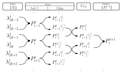
Figure 1: The pictorial description of an iteration. The input is the list of the diagonal elements of the full density matrix, $\{\lambda^{t}\}$. The reset step first merges every two neighbouring elements (partial trace) and then replaces the reset qubit with $\rho_{R}$ which splits each element into two elements again. Next, the $U_{\text{TS}}$ swaps all the neighbouring elements except for the first and the last one.

For simplicity, we focus on the computation qubits and trace out the reset qubit. This gives the following update rule for the diagonal elements of the computation qubits:

$$p_{i}^{t+1}=p_{i-1}^{t}\frac{e^{-\epsilon}}{z}+p_{i+1}^{t}\frac{e^{\epsilon}}{z}.$$ (4)

for $1<i<2^{n}$.

Similarly, for the first and the last elements, the update rules are $p_{1}^{t+1}=(p_{1}^{t}+p_{2}^{t})\frac{e^{\epsilon}}{z}$ and $p_{2^{n}}^{t+1}=(p_{2^{n}-1}^{t}+p_{2^{n}}^{t})\frac{e^{-\epsilon}}{z}$.

These update rules give the following $2^{n}\times 2^{n}$ transition matrix for the Markov process:

$$T=\frac{1}{z}\left(\begin{array}[]{ccccc}e^{\epsilon}&e^{\epsilon}&0&\cdots&0\\ e^{-\epsilon}&0&e^{\epsilon}&\cdots&0\\ 0&e^{-\epsilon}&0&\cdots&0\\ 0&0&\cdots&\ddots&\vdots\\ 0&0&\cdots&e^{-\epsilon}&e^{-\epsilon}\end{array}\right).$$ (5)

It is easy to verify that $\vec{\{p^{t+1}\}}=T\vec{\{p^{t}\}}$ and gives the update rules above. The matrix $T$ has a unique eigenvalue $1$ and the remaining eigenvalues are $\Upsilon_{k}=\frac{2\cos{\frac{k\pi}{2^{n}}}}{z}$ for $k=1,2,\cdots,2^{n}-1$. The eigenstate corresponding to eigenvalue one is

$$\rho=p_{0}\{1,e^{-2\epsilon},e^{-4\epsilon},\cdots\},$$ (6)

which is the OAS and $p_{0}$ is the normalization factor Raeisi and Mosca (2015). For the detailed calculation of the eigensystem, see the Supplemental Material(SM). Since all the other eigenvalues lie in the interval $(1,-1)$, the Markov chain asymptotically converges to $\rho$. This proves that our technique asymptotically achieves the cooling limit of HBAC.

We give a $O\left(n^{2}\right)$ circuit for the implementation of the two-sort unitary in the SM. We first shift the basis by one, which transforms it to $\text{Toff}(n+1)\sigma_{x}^{(n+1)}$. Then a Pauli $\sigma_{x}$ on the reset qubit turns the matrix to a multiple-control Toffoli gate (see SM for details). This shows that our technique can be efficiently implemented. However, to reach the OAS, we need to investigate how many iterations would be required. The mixing time of a Markov chain is the number of iterations required to get within distance $\xi$ of the asymptotic state (i.e. to achieve $|\rho^{t}-\rho_{OAS}|\leq\xi$). We can upper bound this number of iterations as a function of the spectral gap $\Delta$, i.e. the difference between $1$ and the second largest eigenvalue,

$$t_{\text{mix}}\left(\xi\right)\leq\log\left(\frac{1}{\xi\,l}\right)\frac{1}{\Delta},$$ (7)

where $l=p_{0}e^{-(2^{n}-1)\epsilon}$ is the smallest element of the array in Eq. (6) Levin, Peres, and Wilmer (2009).

The spectral gap is $\Delta=1-\left(2\cos{\frac{\pi}{2^{n}}}\right)/\left(e^{\epsilon}+e^{-\epsilon}\right)\geq\frac{z-2}{z}$. This gives

$$t_{\text{mix}}(\xi)\leq\left(\log\left(\frac{1}{\xi\,p_{0}e^{-(2^{n}-1)\epsilon}}\right)\left(\frac{z}{z-2}\right)\right).$$ (8)

It is easy to check that $t_{\text{mix}}\in O(2^{n})$ which yields $O(n^{2}2^{n})$ for the overall complexity of TSAC.

Now, we compare our technique with PPA. The key ingredient of PPA is sorting the diagonal elements of the density matrix in each iteration. This transfers as much entropy as possible from the computation elements to the reset qubit Schulman, Mor, and Weinstein (2005). Then the reset qubit is reset back to its equilibrium state.

Even assuming that finding the operation for sorting a $2^{n+1}$ array is easy, we need to find quantum circuits to implement them which has at least $O(e^{n})$ classical complexity. Note that this is only the classical cost of the algorithm. Without this, it would not be even possible to start implementing PPA. For systems as large as 20-40 qubits, e.g. the experiment in Pande et al. (2017), not only it is challenging to implement PPA, but it also seems difficult to find the required permutations. This is in contrast to our technique, where each iteration is already known and there is a specific circuit for implementing it.

Next is the gate complexity of PPA. Typically only the number of iterations is counted, ignoring the complexity of the sort operations. In fact, due to the complexity of the sort operations, it is difficult to bound the number of gates required for PPA. Naively, there are $(2^{n})!$ permutation matrices of size $2^{n}$. Assuming a finite number of one- and two-qubit gates, there are only $\left[\text{poly}(n)\right]^{d}$ circuits with at most $d$ gates on $n$ qubits. Taking $d$ to be $\text{poly}(n)$, one can see that only a small fraction of permutations can be implemented efficiently. Here, we provide a more rigorous bound on the gate complexity of PPA.

The permutation operations can be decomposed into separate cycles that form disjoint blocks in the permutation matrix. These cycles could have different sizes and the size of each cycle determines the number of states it permutes cyclically. These are known as $k$-cycles, where $k$ is the size of the block.

Assume that for all the $k$-cycles in the permutation, we can find an efficient circuit. Also assume that, given a certain state $\left|j\right\rangle$, it is possible to efficiently determine which block the state belongs to. Furthermore, we assume that cycles of equal size can be implemented in parallel efficiently. These assumptions may not be true, but any lower bound established with these assumptions still holds when any of these assumptions are weakened or dropped. Under these assumptions, the cost would depend on the number of $k$-cycles with distinct $k$ values. This is the number of blocks in the permutation matrix that have different size. We refer to this quantity as NBDS.

Implementation of each sort operation requires the implementation of all the blocks. Blocks of different size cannot be fully parallelized and for switching between each of two blocks of unequal size, some quantum operation would be required. This sets the number of blocks of different size NBDS as a lower bound for the complexity of any sort operation.

Figure (2) shows the simulation results of PPA for a different number of computation qubits, $n$ and indicates that NBDS grows exponentially with $n$. This implies that our lower-bound for the gate complexity of PPA scales exponentially with $n$. Here, for any value of $n$, we get a sequence of permutation matrices and pick the permutation that has the largest NBDS.

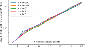
Figure 2: This plot shows that the maximum of the NBDS for implementations of PPA grows exponentially with the number of computation qubits $n$. The $y$ axis a is logarithmic scale. Different plots correspond to different reset polarizations $\epsilon$.

Last, there is the fragility to practical imperfections. The sort operation of PPA requires the ordering of the diagonal elements of the state. This means that techniques like quantum state tomography are needed to monitor the state. This process however, cannot be perfect and usually there are estimation errors. Figure (3) shows how sensitive the process is to these imperfections. These simulations are for HBAC with $n=2$ and one reset qubit and the reset polarization of $\epsilon=0.02$ with a zero-mean Gaussian noise with variance $\sigma$. As $\sigma$ increases, the process becomes random and would not approach the cooling limit any more. Figure (3) also shows the result for TSAC which regardless of the noise, would always converge to the OAS. This is not a generic noise model, but is relevant for techniques like PPA and shows that with noise, PPA can heat the state. Next, we show that TSAC monotonically pushes the state towards the OAS.

Theorem 1.

Given some state $\rho$ and a reset state $\rho_{R}$ with polarization $\epsilon$, if the polarization of the first computation qubit is less than the HBAC limit, each iteration of TSAC, as in equation (3) would increase the polarization of the first qubit.

Proof.

The polarization of the first qubit is determined by the first half of the diagonal elements of $\rho$ and we need to show that TSAC would increase it. The assumption that the state is hotter than the HBAC limit means

$$p_{2^{n-1}}e^{-\epsilon}<p_{2^{n-1}+1}e^{\epsilon}.$$ (9)

After the iteration, these two are swapped by the $U_{\text{TS}}$. This increases the sum of the first half of the diagonal elements and as a result, the polarization of the first qubit. ∎

Note that this can be extended to other computation qubits. It is just easier to show for the first qubit.

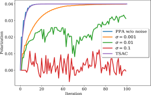
Figure 3: This plot shows the polarization of the first qubit vs iterations. This is for the simulation of PPA for two computation qubits and one reset qubit, with different amounts of the state estimation errors $\sigma$.

Since the process does not depend on the state, even when the state is perturbed from the ideal one, the process continues to cool it down. Note that this does not imply that our algorithm is robust to all imperfections. Specifically, with faulty operations, no algorithm can guarantee the convergence to OAS.

Table (1) gives a comparison between TSAC and PPA. Here, the “noise sensitivity” is the sensitivity to deviations from the expected state in the process. The table demonstrates that TSAC outperforms PPA in almost every aspect and presents a more realistic option in practice.

	PPA	TSAC
Classical cost of circuit synthesis	$\Omega(2^{n})$	$\text{poly}(n)$
Total number of gates	(Conjecture) $\Omega(2^{n})$	$O\left(n^{2}2^{n}\right)$
Noise sensitivity	Sensitive	Robust

Table 1: Comparison between PPA and our technique. Here, the “noise sensitivity" is the sensitivity to deviations from the expected state in the process.

In conclusion, our work presents a novel viable technique for optimal HBAC which shows that optimal HBAC is possible without any knowledge of the state and without changing the operation through the process. From a Quantum Thermodynamics(QT) viewpoint, it means that the optimal cooling is possible to do HBAC with a cyclic process. This opens new avenues for examining HBAC in terms of QT. For instance, resources required for reaching the cooling limit have been extensively investigated in QT Scharlau and Mueller (2016); Allahverdyan et al. (2011); Masanes and Oppenheim (2017); Streltsov et al. (2018); Reeb and Wolf (2014); Browne et al. (2014); Masanes and Oppenheim (2017). It is interesting to map the required resources and their scaling to HBAC.

Our work also brings realistic applications of these techniques to the realm of possibility. The new technique, in contrast to PPA, uses a fixed operation in every iteration, which addresses the fragility issues in previous works. More precisely, the new technique is robust against imperfections and noise in the state.

It is also possible to combine our work with other dynamics cooling techniques to further reduce the costs. However, it remains open to see how far the complexity may be reduced. Results from QT on the analysis of the resources for cooling and the extensions of the third law of thermodynamics Masanes and Oppenheim (2017); Scharlau and Mueller (2016); Allahverdyan et al. (2011); Streltsov et al. (2018) could prove helpful for reducing the complexity of cost.

I Supplementary Material

Spectrum of the transfer matrix

We solve the eigenvalue equation, $T\Phi^{(p)}=\Upsilon\Phi^{(p)}$, indexing the eigenvectors by $p$. Using the sparsity and the structure of $T$, we can rewrite the eigenvalue equations as

$$\Upsilon^{(p)}\Phi_{1}^{(p)} =(\Phi_{1}^{(p)}+\Phi_{2}^{(p)})\frac{e^{\epsilon}}{z},$$ (S1)

$$\Upsilon^{(p)}\Phi_{k}^{(p)} =\Phi_{k-1}^{(p)}\frac{e^{-\epsilon}}{z}+\Phi_{k+1}^{(p)}\frac{e^{\epsilon}}{z},$$ (S2)

$$\Upsilon^{(p)}\Phi_{2^{n}}^{(p)} =(\Phi_{2^{n}-1}^{(p)}+\Phi_{2^{n}}^{(p)})\frac{e^{-\epsilon}}{z},$$ (S3)

for $1<k<2^{n}$. We use the ansatz

$$\Phi_{k}^{(p)}=e^{(ip-\epsilon)k}+\alpha e^{(-ip-\epsilon)k}$$ (S4)

with arbitrary complex parameters $\alpha$ and $p$. This ansatz automatically satisfies S2 with eigenvalue

$$\Upsilon^{(p)}=\frac{2\cos{p}}{e^{\epsilon}+e^{-\epsilon}}.$$ (S5)

We set the value of $\alpha$ by solving S1 and obtain $\alpha=\frac{e^{ip}-e^{-\Delta}}{e^{-\Delta}-e^{-ip}}$. Note that this result forbids $p=0$ because it gives $\Phi_{k}^{(0)}=0$.

At last, we satisfy S3 and obtain allowed values of $p$. The solution $ip=\pm\epsilon$ gives eigenvalue $1$ and corresponds to the eigenvector $\Phi_{k}^{(p)}=e^{-2\Delta k}$. This is the asymptotic state of PPA as was proved in Raeisi and Mosca (2015).

The remaining eigenvalues are of form $\frac{2\cos{\frac{j\pi}{2^{n}}}}{e^{\epsilon}+e^{-\epsilon}}$ for $1\leq j<2^{n}$. All these eigenvalues lie in the range $(-1,1)$. In other words, the Markov chain has a unique eigenvalue one and all the other eigenvalues are smaller than one. Therefore the Markov chain defined by the transition matrix $T$ converges to the +1 eigenvector, which is OAS.

The convergence rate is determined by the difference between $1$ and the second largest eigenvalue, $\Upsilon^{(2)}=\frac{2\cos{\frac{\pi}{2^{n}}}}{e^{\epsilon}+e^{-\epsilon}}$. We can bound the gap as $\Delta=1-\left(2\cos{\frac{\pi}{2^{n}}}\right)/\left(e^{\epsilon}+e^{-\epsilon}\right)\geq\frac{z-2}{z}$. The mixing time is then upper-bounded by

$$t_{\text{mix}}\left(\xi\right)\leq\log\left(\frac{1}{\xi\,l}\right)\frac{1}{\Delta}\leq\left(\log\left(\frac{1}{\xi\,l}\right)\left(\frac{z}{z-2}\right)\right)\leq c_{1}\log\left(\frac{1}{l}\right)+c2,$$ (S6)

where $c_{1}=\left(\frac{z}{z-2}\right)$ and $c_{2}=\left(\frac{z}{z-2}\right)\log\left(\frac{1}{\xi}\right)$ are both constant with respect to $n$. To find the scaling of the upper-bound, we need to calculate the

$$\log\left(\frac{1}{l}\right)=\log\left(\frac{1}{p_{0}e^{-(2^{n}-1)\epsilon}}\right)=\log\left(\frac{(1-(e^{-2\epsilon})^{2^{n}})}{(1-e^{-2\epsilon})e^{-(2^{n}-1)\epsilon}}\right).$$

For the values of $l$ and $p_{0}$ see Raeisi and Mosca (2015).

To understand the scaling, we take $n\gg 1$ which simplifies the bound to

$$\log\left(\frac{1}{e^{-(2^{n}-1)\epsilon}}\right)-c_{3},$$

where $c_{3}=\log\left(1-e^{-2\epsilon}\right)$. So the scaling of the upper-bound is $O(2^{n})$.

The Circuit for $U_{\text{TS}}$

The unitary that sorts the density matrix lexicographically is

$$U_{\text{TS}}=\begin{pmatrix}1&0&0&0&0&\cdots&0&0&0\\ 0&0&1&0&0&\cdots&0&0&0\\ 0&1&0&0&0&\cdots&0&0&0\\ 0&0&0&0&1&\cdots&0&0&0\\ 0&0&0&1&0&\cdots&0&0&0\\ \vdots&\vdots&\vdots&\vdots&\vdots&\ddots&\vdots&\vdots&\vdots\\ 0&0&0&0&0&\cdots&0&1&0\\ 0&0&0&0&0&\cdots&1&0&0\\ 0&0&0&0&0&\cdots&0&0&1\end{pmatrix}.$$ (S7)

$U$ is a block diagonal $2^{n}\times 2^{n}$ matrix with $1\times 1$ blocks in the upper left and lower right corners and the other blocks are $X=\begin{pmatrix}0&1\\ 1&0\end{pmatrix}$.

The first and the last operations are SHIFT_m operators which are defined as

$$\text{SHIFT}_{m}\left|x_{1}x_{2}\dots x_{n}\right\rangle=\left|\left(x_{1}x_{2}\dots x_{n}+m\right)mod2^{n}\right\rangle.$$ (S8)

This notation is mostly symbolic but should be understood as binary addition between strings labeling states on $n$ qubits. For example, SHIFT${}_{1}\left|101\right\rangle=\left|110\right\rangle$. The other operations are multiple-control-Toffoli, Toff_n, which is a controlled NOT with $n-1$ controls and NOT (Pauli X) on the last qubit.

NOTs are easy to implement and for SHIFT₁ and Toff_n we use the construction in Saeedi and Pedram (2013).

After Toff_n we apply NOT on the last qubit. Multiple-control-Toffoli and NOT give together the unitary

$$U^{\prime}=\begin{pmatrix}0&1&0&0&\cdots&0&0&0&0\\ 1&0&0&0&\cdots&0&0&0&0\\ 0&0&0&1&\cdots&0&0&0&0\\ 0&0&1&0&\cdots&0&0&0&0\\ \vdots&\vdots&\vdots&\vdots&\ddots&\vdots&\vdots&\vdots&\vdots\\ 0&0&0&0&\cdots&0&1&0&0\\ 0&0&0&0&\cdots&1&0&0&0\\ 0&0&0&0&\cdots&0&0&1&0\\ 0&0&0&0&\cdots&0&0&0&1\\ \end{pmatrix}.$$ (S9)

Therefore, to apply U, we must shift all the rows and columns of $U^{\prime}$ cyclically. This is what SHIFT₊₁ and its conjugate transpose SHIFT_-1 do. We can implement SHIFT₊₁ with Quantum Fourier Transform and rotations Beth and Rötteler (2001). In Fig (S1), we show how to implement a more general operation, SHIFT_+m.

In this circuit, first, QFT^-1 transforms the bit-strings from registers to phases

$$\left|x_{1}\right\rangle\left|x_{2}\right\rangle\dots\left|x_{n}\right\rangle\rightarrow\frac{1}{\sqrt{2^{n}}}\left(\left|0\right\rangle+e^{2\pi i\frac{x_{1}x_{2}\dots x_{n}}{2^{n}}}\left|1\right\rangle\right)\left(\left|0\right\rangle+e^{2\pi i\frac{x_{2}\dots x_{n}}{2^{n-1}}}\left|1\right\rangle\right)\cdots\left(\left|0\right\rangle+e^{2\pi i\frac{x_{n}}{2}}\left|1\right\rangle\right).$$ (S10)

In the next step, we apply rotations around $z$ on each qubit. This yields

$$\frac{1}{\sqrt{2^{n}}}\left(\left|0\right\rangle+e^{2\pi i\frac{x_{1}x_{2}\dots x_{n}+m}{2^{n}}}\left|1\right\rangle\right)\left(\left|0\right\rangle+e^{2\pi i\frac{x_{2}\dots x_{n}+m}{2^{n-1}}}\left|1\right\rangle\right)\cdots\left(\left|0\right\rangle+e^{2\pi i\frac{x_{n}+m}{2}}\left|1\right\rangle\right).$$ (S11)

After applying the Quantum Fourier Transform, we get the desired state $\left|x_{1}x_{2}\dots x_{n}+m\right\rangle$.

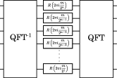
Figure S1: The circuit for the SHIFT operator in Eq. (S8).

Complexity of the sort operations in PPA

First, note that the implementation cost of a sort operation could in general be exponential in $n$. Here we give a lower bound for the implementation cost that takes into account the cost of the sort operations. We use numerical evidence to show that the lower-bound scales exponentially with $n$.

A permutation matrix basically permutes the basis and we need to find the circuit with the minimum number of gates that gives the same basis transformation. Clearly, mapping every element of the basis would be exponential in $n$ since there are $2^{n}$ basis to map. So we need to parallelize as many mappings as possible.

As explained in the text, we assume that all the cycles of the permutation have efficient implementation and for cycles of the same size, it is easy to implement them in parallel. Without parallelizing the implementation of blocks that have different sizes, the complexity would be proportional to the number of blocks with different size (NBDS).

The numerical evidence presented in figure (5) in the text, shows that NBDS scales exponentially with $n$.

Non-diagonal density matrices

It is possible that the density matrix becomes non-diagonal during the cooling process due to the noise in the system. Here we show that our technique can handle non-diagonal density matrices as well and would take them to the OAS.

We show that the presence of any non-diagonal elements will not affect the action of $U_{\text{TS}}$ on the diagonal of the density matrix. In other words, the same permutation is applied on the diagonal elements even if the density matrix is non-diagonal in computational basis.

We can write $U_{\text{TS}}$ as

$$U_{\text{TS}}=\left|0\right\rangle\left\langle 0\right|+\left|2^{n}-1\right\rangle\left\langle 2^{n}-1\right|+\sum_{i\in odd}^{2^{n}-2}{(\left|i+1\right\rangle\left\langle i\right|+\left|i\right\rangle\left\langle i+1\right|)}.$$ (S12)

Now, if we apply the evolution to some arbitrary density matrix $\rho=\sum_{i,j}{\rho_{ij}\left|i\right\rangle\left\langle j\right|}$, for the diagonal elements we get

$$\left\langle i\right|U_{\text{TS}}\rho U^{\dagger}_{\text{TS}}\left|i\right\rangle=\rho_{0,0}\left|0\right\rangle\left\langle 0\right|+\rho_{2^{n}-1,2^{n}-1}\left|2^{n}-1\right\rangle\left\langle 2^{n}-1\right|+\sum_{i\in odd}{(\rho_{i,i}\left|i+1\right\rangle\left\langle i+1\right|+\rho_{i+1,i+1}\left|i\right\rangle\left\langle i\right|)}.$$ (S13)

The first two terms show that the first and last elements of the diagonal elements of the density matrix are preserved, while the last term indicates that for all odd values of $i$, we get $\rho_{i,i}\leftrightarrow\rho_{i+1,i+1}$. This gives the same permutation for the diagonal element as for a diagonal density matrix. This means that the diagonal element would again follow a time-independent Markov chain given by the same transfer matrix, T (Eq. (5) of the main text).

Note that polarization only depends on the diagonal elements of the density matrix, so it suffices to focus on the dynamics of these diagonal elements. As was shown here, this dynamics would be the same regardless of off-diagonal elements of the density matrix.

Robustness

Here we included some additional numerical simulation for the noise model investigated in figure (3) of the main body, for larger $n$ and polarization, $\epsilon$. Specifically, we redid the simulation of PPA for $n=10$ computation and one reset qubit, and for polarization of $0.1$ and with $\sigma=0.1,0.15,0.2$.

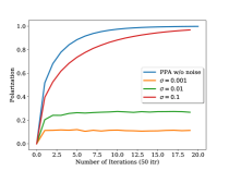
Figure S2: This plot shows the polarization of the first qubit vs. iterations. This is for the simulation of PPA for $10$ computation and one reset qubit, polarization of $0.1$ and with different amounts of the state estimation errors, $\sigma$ indicated in the legend of the plot.

Practical Imperfections

Here we discuss imperfections for practical applications.

There are two mechanisms for error that can be distinguished.

The first is due to the deviation between the state we assume we have and the state we actually have. PPA uses information about the state to find the required sort operation for each iteration. This is in contrast to TSAC which operates independently of the state. This is the notion of robustness that was discussed in the main body.

Second are errors directly introduced by errors in the implementation of the required operations. As we mentioned in the main body of this paper, it is not clear how either of these two techniques would handle such imperfections.

Here we sketch an approach for attempting to analyze robustness in more detail, why we expect TSAC to be more resilient than PPA against certain types of noise, and some of the challenges with analyzing the various possible noise models.

With ideal PPA, the ideal input state $\rho=\rho_{0}$ undergoes a series of unitary transformations $U_{1},U_{2},\ldots,U_{j},\ldots$, with a reset step in between, so that $\rho_{j}=U_{j}\mathcal{R}(\rho_{j-1})U_{j}^{\dagger}$ where $\mathcal{R}$ denotes the reset step (where the reset qubits are given time to re-equilibrate and ideally nothing happens to the computation qubits) and the compression operator $U_{j}$ depends on the state $\rho_{j-1}$.

With ideal TSAC the ideal input state $\rho=\rho_{0}$ repeatedly undergoes the same unitary transformations $U$ (that does not depend on the input state), with a reset step in between, so $\rho_{j}=U\mathcal{R}(\rho_{j-1})U^{\dagger}$.

A noisy PPA may be modelled as instead mapping (where $\rho_{0}^{\prime}=\rho_{0}$)

$$\rho_{j-1}^{\prime}\mapsto\rho_{j}^{\prime}=U_{j}C_{j}(\mathcal{R}(\rho_{j-1}^{\prime}))U_{j}^{\dagger}$$

for some completely positive map $C_{j}$.

Similarly a noisy TSAC may be modelled as instead mapping

$$\rho_{j-1}^{\prime}\mapsto\rho_{j}^{\prime}=UC(\mathcal{R}(\rho_{j-1}^{\prime}))U^{\dagger}$$

for some completely positive map $C$.

In these characterizations, the $C_{j}$ (or $C$) operators wlog capture the noise or imperfections while attempting to implement the ideal $U_{j}$ (or $U$) and we assume also capture the deviation between the ideal reset operation and the actual reset transformation. We note that technically not all imperfect implementations can be decomposed in this way. However, for the sake of just outlining our intuition here, we will model the noise this way (and we also note that we expect that an actual physical system designed to approximate the HBAC assumptions would have a reset operation that can be closely approximated by the ideal reset operation followed by additional noise on the reset and computation qubits).

The noise operators $C_{j}$ (or $C$) can affect the cooling process in two ways. First, they can reduce the purity and directly heat up the state (e.g. a depolarizing channel would do this). Second, the change in the state may make the subsequent cooling operation ineffective or even lead to cause heating.

More specifically, with PPA, the ideal $U_{1}$ is designed to sort the diagonal elements of $\mathcal{R}(\rho_{0})$ and thereby cool the state. However, if the diagonal elements of $C_{1}(\mathcal{R}(\rho_{0}))$ have a different order, PPA could end up heating the state. Similarly, subsequent $U_{j}$ are designed to cool the ideal input state $\mathcal{R}(\rho_{j-1})$, but may in fact end up heating up the actual state $C(\mathcal{R}(\rho_{j-1}^{\prime}))$ that has been impacted by imperfect operations.

For the first effect, i.e. the direct heating caused by the noise channel, one could hope that if the heating rate of $C_{j}$ (or $C$) is less than the cooling rate of $U_{j}$ (or $U$), we could show that $U_{j}C_{j}(\mathcal{R}(\rho_{j-1}^{\prime}))U_{j}^{\dagger}$ (or $UC(\mathcal{R}(\rho_{j-1}^{\prime}))U^{\dagger}$) would still improve the purity compared to $\mathcal{R}(\rho_{j-1}^{\prime})$. However, both the heating rate of $C_{j}$ (or $C$) and cooling rate of $U_{j}$ (or $U$) depend on their input states, making it challenging to determine if there is a net cooling or heating after both operations are applied.

For the second effect, TSAC seems to have an advantage compared to PPA. Theorem (1) in the main text implies that, assuming $C_{j}(\mathcal{R}(\rho_{j-1}^{\prime}))$ is hotter than the optimal asymptotic state (OAS), then $UC_{j}(\mathcal{R}(\rho_{j-1}^{\prime}))U^{\dagger}$ would have a lower temperature than $C_{j}(\mathcal{R}(\rho_{j-1}^{\prime}))$. But it may not necessarily have a lower temperature than $\mathcal{R}(\rho_{j-1}^{\prime})$. In contrast, for techniques like PPA, since the compression is designed for the idea $\rho_{j-1}$, it may not only be ineffective for $C_{j}(\mathcal{R}(\rho_{j-1}^{\prime}))$ but it may even heat it up.

In summary, we have outlined some intuition on the complexity of analyzing imperfections in the implementation of compression operators, and why there may exist noise models under which the noisy implementation would heat the state, and other noise models where the state would get cooled. This topic needs further investigation.