A study of the nonlinear optical response of the plain graphene and gapped graphene monolayers beyond the Dirac approximation

Abstract

In this work, we present numerical results for the second and third order conductivities of the plain graphene and gapped graphene monolayers associated with the second and third harmonic generation, the optical rectification and the optical Kerr effect. The frequencies considered here range from the microwave to the ultraviolet portion of the spectrum, the latter end of which had not yet been studied. These calculations are performed in the velocity gauge and directly address the components of the conductivity tensor. In the velocity gauge, the radiation field is represented by a power series in the vector potential, and we discuss a very efficient way of calculating its coefficients in the context of tight-binding models.

I Introduction

It has now been over a decade since the publication of the theoretical works of S. A. Mikhailov on the low-frequency (intraband) nonlinear response of the monolayer of graphene to an external electric field (Mikhailov, 2007; Mikhailov and Ziegler, 2008), which marked the birth of the study of nonlinear optical (NLO) responses in two-dimensional materials. In the past ten years, this area has become increasingly active and diverse, as it gathered the attention of both theoretical (Al-Naib et al., 2014; Glazov and Ganichev, 2014; Peres et al., 2014; Cheng et al., 2014, 2015a, 2015b; Mikhailov, 2016; Semnani et al., 2016; Mikhailov, 2017; Savostianova and Mikhailov, 2017; Ventura et al., 2017; Passos et al., 2018; Savostianova and Mikhailov, 2018; Hipolito et al., 2018) and experimental groups (Hendry et al., 2010; Dean and van Driel, 2010; Zhang et al., 2012; Kumar et al., 2013; Hong et al., 2013; Dremetsika et al., 2016; Vermeulen et al., 2016; Higuchi et al., 2017; Baudisch et al., 2018). This has also been extended to many other, more recently isolated, layered materials (Janisch et al., 2014; Pedersen, 2015; Hipolito et al., 2016; Hipolito and Pedersen, 2018; Youngblood et al., 2017). In those materials, like in graphene, the nonlinear optical response has been shown to be very intense, much more so than in three dimensional materials.

One key issue, that followed directly from those initial works, was to expand the understanding of the nonlinear intraband response — frequencies in the microwave and the infrared — into the high frequency range — frequencies in the near infrared and above (Cheng et al., 2014, 2015a, 2015b; Mikhailov, 2016). Doing so required a full quantum treatment of the electrons in a crystal, and meant recovering the formalism for the calculation of NLO coefficients in bulk semiconductors of the late eighties and early nineties, developed by J. E. Sipe and collaborators (Moss et al., 1989; Sipe and Ghahramani, 1993; Aversa and Sipe, 1995; Sipe and Shkrebtii, 2000). Their work, mostly formulated in the so-called length gauge, provided expressions for the second and third order optical conductivities that are directly applicable to a system of non-interacting electrons in a solid, taking both intraband and interband transitions into account. Many other works have since used this framework. In practice, due to the complexity of the general expressions, calculations of nonlinear optical conductivities usually require performing the analytical calculation (i.e., an integration over the FBZ) for the particular system under study: in third order this is already rather cumbersome. Often, it is only really tractable for simple effective Hamiltonians (such as the Dirac Hamiltonian in graphene), that describe only a portion of the FBZ. This has limited the length gauge method to sufficiently small frequencies for such effective Hamiltonians to be applicable.

Another approach, based on the velocity gauge, was developed concurrently but presented early difficulties. Spurious divergences and inaccurate results upon the truncation of the number of bands led the velocity gauge to be less adopted. The origin of these difficulties was understood early on as a violation of sum rules (Aversa and Sipe, 1995). This was solved only recently (Passos et al., 2018), with a reformulation of the velocity gauge that is able to reproduce the results from the length gauge and that is best suited for numerical calculations that involve the full FBZ. Two diagrammatic methods based on this formulation of the velocity gauge have since been developed (Parker et al., 2019; João and Lopes, 2018), the former of which was used in the study of Weyl semimetals, while the latter was shown to be applicable even in disordered systems. In this velocity gauge approach there is no added dificulty in moving to higher frequencies and in fact its implementation requires the use of models defined in the entire FBZ. The authors will use the new velocity gauge approach of ref.(Passos et al., 2018) to probe the NLO response of graphene in a frequency range beyond the Dirac approximation.

We present numerical results for the second and third order responses of the plain graphene (PG) and gapped (GG) graphene monolayers to a monochromatic electric field of frequencies (energies) that range from the microwave ($\hbar\omega\sim 0.005$ eV) to the ultraviolet ($\hbar\omega\sim 6$ eV). These results differ from what has been previously reported in literature (Cheng et al., 2014, 2015b, 2015a; Mikhailov, 2016; Passos et al., 2018; Hipolito et al., 2018) for two reasons: we go beyond the Dirac cone approximation (valid up to about 1 eV) and study the response of the PG and GG monolayers at high frequencies. Our calculations address all different components of the conductivity tensors — on which intrinsic permutation symmetry is imposed — and not the effective tensors of ref.(Hipolito et al., 2018), which also goes beyond the Dirac approximation, but where Kleinman’s symmetry is additionally imposed. Since this second symmetry follows from the consideration that the nonlinear susceptibilities (or conductivities) can be deemed dispersionless (Boyd, 2008), it lacks justification in the study of the response in these frequency ranges. Although seemingly technical in nature, this difference is practically relevant as the conductivities computed here can be directly related to measurements of the current response, $J^{\alpha}(t)$, in an experiment (regardless of the polarization of the electric field), whereas the effective tensors cannot.

The paper is organized as follows. In the following section, we perform a review of the calculations of NLO conductivities in the length and the velocity gauges. Section III is dedicated to the use of tight-binding Hamiltonians in velocity gauge calculations and to two pertinent points: the computation of $h$ coefficients, which are integral to the description of the response in the velocity gauge become simple when working on a basis for which the Berry connections are all trivial; the second point concerns the relation between these Berry connections and the manner by which one defines the position operator in the lattice. It is shown that this has implications in the optical response by studying the interband portion of the linear conductivity of plain graphene. In Section IV, we present the aforementioned results, i.e., the second harmonic generation and optical rectification conductivities, of the GG monolayer and for the third order response, i.e., the harmonic generation and Kerr effect conductivities, of the PG and GG monolayers, in the aforementioned frequency regime. For the two second order effects the results are complemented by analytical calculations of the real part of the conductivities. The final section is dedicated to a summary of our work.

II Calculation of nonlinear optical conductivities in crystals

A system’s nonlinear current response to a monochromatic electric field, that is considered to be constant throughout the material,

$$\mathbf{E}(t)= \mathbf{E}_{0}\,e^{i\omega t}+\left(\mathbf{E}_{0}\right)^{*}\,e^{-i\omega t}$$ (1)

is described, in second order, by the second harmonic generation, $\sigma_{\beta\alpha_{1}\alpha_{2}}^{(2)}(\omega,\omega)$, and the optical rectification, $\sigma_{\beta\alpha_{1}\alpha_{2}}^{(2)}(\omega,-\omega)$, conductivities,

$$J_{\beta}^{(2)}(t)= \ \sigma_{\beta\alpha_{1}\alpha_{2}}(\omega,\omega)\,E_{0}^{\alpha_{1}}\,E_{0}^{\alpha_{2}}\,e^{-i2\omega t}$$

$$+\sigma_{\beta\alpha_{1}\alpha_{2}}(\omega,-\omega)\,E_{0}^{\alpha_{1}}\,(E_{0}^{\alpha_{2}})^{*}$$

$$+\text{c.c.},$$ (2)

while, in third order, it is described by the third harmonic generation, $\sigma_{\beta\alpha_{1}\alpha_{2}\alpha_{3}}^{(2)}(\omega,\omega,\omega)$ and the Kerr effect, $\sigma_{\beta\alpha_{1}\alpha_{2}\alpha_{3}}^{(3)}(\omega,\omega,-\omega)$, conductivities,

$$J_{\beta}^{(3)}(t)= \ \sigma_{\beta\alpha_{1}\alpha_{2}\alpha_{3}}(\omega,\omega,\omega)\,E_{0}^{\alpha_{1}}\,E_{0}^{\alpha_{2}}\,E_{0}^{\alpha_{3}}\,e^{-i3\omega t}$$

$$+\sigma_{\beta\alpha_{1}\alpha_{2}\alpha_{3}}(\omega,\omega,-\omega)\,E_{0}^{\alpha_{1}}\,E_{0}^{\alpha_{2}}\,(E_{0}^{\alpha_{3}})^{*}\,e^{-i\omega t}$$

$$+\text{c.c.},$$ (3)

The problem of studying $J_{\alpha}^{(n)}(t)$ is thus a problem of knowing how to calculate the conductivities, $\sigma^{(n)}$, by means of a perturbative expansion. This topic has been the subject of intense research for crystalline systems (Moss et al., 1989; Sipe and Ghahramani, 1993; Aversa and Sipe, 1995; Sipe and Shkrebtii, 2000; Cheng et al., 2014; Mikhailov, 2016; Ventura et al., 2017; Passos et al., 2018) and we will use, in particular, results of our previous work (Ventura et al., 2017; Passos et al., 2018), in the following review of those calculations. The baseline considerations here are the same as before: the electric field is constant throughout the crystal and electron-electron interactions, integral to a description of an excitonic response, are not taken into account.

II.1 Crystal hamiltonian and its perturbations

In a perfect infinite crystal, the eigenfunctions of the unperturbed (crystal) Hamiltonian, $H_{0}$, are, according to Bloch’s theorem, written in terms of a plane wave and a function that is periodic in the real space unit cell,

$$\psi_{\mathbf{k}s}(\mathbf{r})= \ e^{i\mathbf{k}\cdot\mathbf{r}}\,u_{\mathbf{k}s}(\mathbf{r}),$$ (4)

for $\mathbf{R}$, any lattice vector,

$$u_{\mathbf{k}s}(\mathbf{r})= u_{\mathbf{k}s}(\mathbf{r}+\mathbf{R}).$$ (5)

Each of these eigenfunctions and its corresponding eigenvalue, $\epsilon_{\mathbf{k}s}$, is labelled by a crystal momentum, $\mathbf{k}$, that runs continuously throughout the first Brillouin zone (FBZ) and by the $s$ index, indicating the band. For a $d$ dimensional crystal, their normalization reads,

$$\left\langle\psi_{\mathbf{k}s}\right|\left.\psi_{\mathbf{k}^{\prime}s^{\prime}}\right\rangle= (2\pi)^{d}\,\delta_{ss^{\prime}}\,\delta(\mathbf{k}-\mathbf{k}^{\prime}).$$ (6)

Furthermore, the periodic part of the Bloch functions (for a fixed $\mathbf{k}$) also forms an orthogonal basis, with an inner product that is defined over the real space unit cell, instead of the entire crystal,

$$\left\langle u_{\mathbf{k}s}\right|\left.u_{\mathbf{k}s^{\prime}}\right\rangle= \frac{1}{v_{c}}\int_{v_{c}}d^{3}\mathbf{r}\,u_{\mathbf{k}s}^{*}(\mathbf{r})\,u_{\mathbf{k}s^{\prime}}(\mathbf{r})=\delta_{ss^{\prime}}.$$ (7)

One can then write the full Hamiltonian, composed of the crystal Hamiltonian and the coupling of the electrons to the external electric field, in the single particle basis of band states. The explicit form of the coupling depends on the representation one chooses for the electric field in terms of the scalar ($\phi(\mathbf{r},t)$) and vector potential ($\mathbf{A}(\mathbf{r},t)$), i.e., on the chosen gauge.

For the length gauge, the vector potential is set to zero,

$$\mathbf{E}(t)=-\nabla\phi(\mathbf{r},t),$$ (8)

and the coupling to the electrons is performed via dipole interaction, $V_{\mathbf{k}ss^{\prime}}^{E}(t)$,

$$H^{E}= \ \int\frac{d^{d}\mathbf{k}}{(2\pi)^{d}}\sum_{s,s^{\prime}}\left|\psi_{\mathbf{k}s}\right\rangle\bigl{[}\epsilon_{\mathbf{k}s}\,\delta_{ss^{\prime}}+V_{\mathbf{k}ss^{\prime}}^{E}(t)\bigr{]}\left\langle\psi_{\mathbf{k}s^{\prime}}\right|,$$ (9)

where,

$$V_{\mathbf{k}ss^{\prime}}^{E}(t)= \ ie\mathbf{E}(t)\cdot\mathbf{D}_{\mathbf{k}ss^{\prime}}.$$ (10)

The covariant derivative, $\mathbf{D}_{\mathbf{k}ss^{\prime}}$, is defined as (Ventura et al., 2017),

$$\mathbf{D}_{\mathbf{k}ss^{\prime}}= \ \nabla_{\mathbf{k}}\delta_{ss^{\prime}}-i\boldsymbol{\xi}_{\mathbf{k}ss^{\prime}},$$ (11)

for $\boldsymbol{\xi}_{\mathbf{k}ss^{\prime}}$, the Berry connection between band states (Blount, 1962),

$$\boldsymbol{\xi}_{\mathbf{k}ss^{\prime}}= \ i\left\langle u_{\mathbf{k}s}\right|\left.\nabla_{\mathbf{k}}u_{\mathbf{k}s^{\prime}}\right\rangle.$$ (12)

As for the velocity gauge, it is the scalar potential that is set to zero,

$$\mathbf{E}(t)= -\partial_{t}\mathbf{A}(t),$$ (13)

and the full Hamiltonian in this gauge, $H^{A}$, is obtained from $H^{E}$ by means of a time-dependent unitary transformation (Passos et al., 2018; Ventura et al., 2017),

$$H^{A}= \int\frac{d^{d}\mathbf{k}}{(2\pi)^{d}}\sum_{s,s^{\prime}}\left|\psi_{\mathbf{k}s}\right\rangle\bigl{[}\epsilon_{\mathbf{k}s}\,\delta_{ss^{\prime}}+V_{\mathbf{k}ss^{\prime}}^{A}(t)\bigr{]}\left\langle\psi_{\mathbf{k}s^{\prime}}\right|,$$ (14)

for a perturbation, $V_{\mathbf{k}ss^{\prime}}^{A}(t)$, that is written as an infinite series in the external field,

$$V_{\mathbf{k}ss^{\prime}}^{A}(t)= \sum_{n=1}^{\infty}\frac{e^{n}}{n!}\,A_{\alpha_{1}}(t)(...)A_{\alpha_{n}}(t)\,h_{\mathbf{k}ss^{\prime}}^{\alpha_{1}(...)\alpha_{n}}.$$ (15)

The coefficients in that expansion, $h_{\mathbf{k}ss^{\prime}}^{\alpha_{1}(...)\alpha_{n}}$, are given by nested commutators of the covariant derivative, Eq.(11), with the unperturbed Hamiltonian (Passos et al., 2018),

$$h_{\mathbf{k}ss^{\prime}}^{\alpha_{1}(...)\alpha_{n}}= \left\langle u_{\mathbf{k}s}\right|(\nabla_{\mathbf{k}}^{\alpha_{n}}...\nabla_{\mathbf{k}}^{\alpha_{1}}H_{0\mathbf{k}})\left|u_{\mathbf{k}s^{\prime}}\right\rangle,$$ (16)

$$= \frac{1}{\hbar^{n}}\bigl{[}D_{\mathbf{k}}^{\alpha_{n}},\bigl{[}(...),\bigl{[}D_{\mathbf{k}}^{\alpha_{1}},\,H_{0}\bigr{]}\bigr{]}\,(...)\bigr{]}_{ss^{\prime}},$$ (17)

with the first one being the velocity matrix element in the unperturbed system. Finally, one can write the velocity operator in each of the gauges: $v^{\beta}=\hbar^{-1}\left[D^{\beta},H\right]$. In the single particle basis, they read as

$$v^{E,\beta}= \int\frac{d^{d}\mathbf{k}}{(2\pi)^{d}}\sum_{s,s^{\prime}}\left|\psi_{\mathbf{k}s}\right\rangle v_{\mathbf{k}ss^{\prime}}^{(0),\beta}\left\langle\psi_{\mathbf{k}s^{\prime}}\right|,$$ (18)

$$v^{A,\beta}(t)= \int\frac{d^{d}\mathbf{k}}{(2\pi)^{d}}\sum_{s,s^{\prime}}\left|\psi_{\mathbf{k}s}\right\rangle\Bigl{[}v_{\mathbf{k}ss^{\prime}}^{(0),\beta}+\sum_{n=1}^{\infty}\frac{e^{n}}{n!}\,$$

$$\times A_{\alpha_{1}}(t)(...)A_{\alpha_{n}}(t)\,h_{\mathbf{k}ss^{\prime}}^{\beta\alpha_{1}(...)\alpha_{n}}\Bigr{]}\left\langle\psi_{\mathbf{k}s^{\prime}}\right|.$$ (19)

II.2 Density matrix and conductivities

The electric current density in the crystal is given by the ensemble average of the velocity operator times the charge of an electron,

$$\langle J^{\beta}\rangle(t)= \ (-e)\,\text{Tr}\left[v^{\beta}\rho(t)\right],$$ (20)

$$= \ (-e)\int\frac{d^{d}\mathbf{k}}{(2\pi)^{d}}\sum_{s,s^{\prime}}v_{\mathbf{k}s^{\prime}s}^{\beta}\,\rho_{\mathbf{k}ss^{\prime}}(t),$$ (21)

and it is written in terms of the matrix elements of the density matrix (DM), whose time evolution is described by the Liouville equation,

$$(i\hbar\partial_{t}-\Delta\epsilon_{\mathbf{k}ss^{\prime}})\rho_{\mathbf{k}ss^{\prime}}(t)= \left[V_{\mathbf{k}},\,\rho_{\mathbf{k}}(t)\right]_{ss^{\prime}}.$$ (22)

Each gauge has its own set of equations of motion, following from the perturbations of Eqs.(10) and (15). The perturbative treatment of the current response requires an expansion of the $\rho_{\mathbf{k}ss^{\prime}}(t)$ in powers of the electric field and solving — recursively — the equations of motion for the matrix elements of the DM, Eq.(22), in frequency space. For the velocity gauge, it also requires an expansion of the velocity matrix elements, Eq.(19), since these also depend on the electric field. At the end of that procedure (Passos et al., 2018; Ventura et al., 2017), one obtains the conductivities of arbitrary order $n$ in both the length and velocity gauges. Here we only present the expressions for the second order conductivities, following the scattering prescription described in (Passos et al., 2018),

$$\sigma_{\beta\alpha_{1}\alpha_{2}}^{(2),E}(\omega_{1},\omega_{2})= e^{3}\int\frac{d^{d}\mathbf{k}}{(2\pi)^{d}}\sum_{s,s^{\prime}}\frac{h_{\mathbf{k}s^{\prime}s}^{\beta}}{\hbar\omega_{12}+2i\gamma-\Delta\epsilon_{\mathbf{k}ss^{\prime}}}$$

$$\ \times\bigl{[}D_{\mathbf{k}}^{\alpha_{1}},\frac{1}{\hbar\omega_{2}+i\gamma-\Delta\epsilon}\circ\bigl{[}D_{\mathbf{k}}^{\alpha_{2}},\rho_{\mathbf{k}}^{(0)}\bigr{]}\bigr{]}_{\mathbf{k}ss^{\prime}}$$

$$+(\{\alpha_{1},\omega_{1}\}\leftrightarrow\{\alpha_{2},\omega_{2}\}),$$ (23)

$$\sigma_{\beta\alpha_{1}\alpha_{2}}^{(2),A}(\omega_{1},\omega_{2})= \frac{e^{3}}{\omega_{1}\omega_{2}}\int\frac{d^{d}\mathbf{k}}{(2\pi)^{d}}\sum_{s,s^{\prime}}\bigl{[}\frac{h_{\mathbf{k}s^{\prime}s}^{\beta}}{\hbar\omega_{12}+2i\gamma-\Delta\epsilon_{\mathbf{k}ss^{\prime}}}\bigl{(}\bigl{[}h_{\mathbf{k}}^{\alpha_{1}},\frac{1}{\hbar\omega_{2}+i\gamma-\Delta\epsilon}\circ\bigl{[}h_{\mathbf{k}}^{\alpha_{2}},\rho_{\mathbf{k}}^{(0)}\bigr{]}\bigr{]}_{\mathbf{k}ss^{\prime}}+\frac{1}{2}\bigl{[}h_{\mathbf{k}}^{\alpha_{1}\alpha_{2}},\rho_{\mathbf{k}}^{(0)}\bigr{]}_{\mathbf{k}ss^{\prime}}\bigr{)}$$

$$+h_{\mathbf{k}s^{\prime}s}^{\beta\alpha_{1}}\,\frac{1}{\hbar\omega_{2}+i\gamma-\Delta\epsilon_{\mathbf{k}ss^{\prime}}}\bigl{[}h_{\mathbf{k}}^{\alpha_{2}},\rho_{\mathbf{k}}^{(0)}\bigr{]}_{\mathbf{k}ss^{\prime}}+\frac{1}{2}h_{\mathbf{k}s^{\prime}s}^{\beta\alpha_{1}\alpha_{2}}\,\rho_{\mathbf{k}ss^{\prime}}^{(0)}\ +(\{\alpha_{1},\omega_{1}\}\leftrightarrow\{\alpha_{2},\omega_{2}\})\bigr{]}.$$ (24)

In the absence of an electric field, the zeroth order DM matrix element is given by the Fermi-Dirac distribution and the band space identity matrix,

$$\rho_{\mathbf{k}ss^{\prime}}^{(0)}=f(\epsilon_{\mathbf{k}s})\,\delta_{ss^{\prime}}.$$ (25)

The equivalence between these two conductivities, as well as for conductivities at an arbitrary order $n$, is ensured by the existence of sum rules (Sipe and Ghahramani, 1993; Passos et al., 2018), that are valid as long as the integration over $\mathbf{k}$ is taken over the full FBZ. Though it is still possible to perform calculations using only a portion of the FBZ — e.g., graphene in the Dirac cone approximation (Cheng et al., 2014, 2015b, 2015a; Mikhailov, 2016, 2017) — one must do so in the length gauge (Ventura et al., 2017), making it the suitable choice for analytical calculations (Passos et al., 2018). In this work we present two analytical results, for the effects of second harmonic generation and optical rectification, in the clean limit: $\gamma\rightarrow 0$.

The velocity gauge, on the other hand, is suitable for numerical approaches that involve the entire FBZ (Passos et al., 2018). It does not feature higher order poles, and it avoids having to take derivatives of the density matrix. Instead, for a response of order $n$, one has to compute all $h$ coefficients, Eq.(16), up to order $n+1$, $h_{\mathbf{k}ss^{\prime}}^{\alpha_{1}...\alpha_{n+1}}$. All numerical results in this paper were calculated in the velocity gauge.

III velocity gauge for Tight-Binding Hamiltonians

A perturbative description of the response in the velocity gauge is correct only if the unperturbed Hamiltonian is defined in the full FBZ. For the purpose of this work, we consider it to be a tight-binding model. This section is therefore dedicated to two points that concern this type of Hamiltonian: we show that the calculation of $h$ coefficients is made simple when one chooses a basis for which all Berry connections are trivial; we also trace the source of variations in the calculations of these coefficients, and to the Berry connections found in the literature, to subtle changes in the definition of the position operator. This difference is illustrated in the linear optical response of the plain graphene monolayer.

III.1 Covariant derivatives in the second Bloch basis

A tight-binding model is a simplified description of electrons in a lattice, where electronic motion is characterized by hoppings from one orbital to its neighbouring ones ($t_{ij}\left(\mathbf{R}_{n},\mathbf{R}_{m}\right)$), where $i,j$ index different orbitals of the same unit cell, which may have distinct on-site energies ($\epsilon_{i}$). In real space,

$$\mathcal{H}= \underset{\mathbf{R}_{n},\,\mathbf{R}_{n},\,i,\,j}{\sum\sum}\left[\,t_{ij}(\mathbf{R}_{n},\mathbf{R}_{m})\bigl{|}\phi_{\mathbf{R}_{n}\,i}\bigr{\rangle}\bigl{\langle}\phi_{\mathbf{R}_{m}\,j}\bigr{|}+\text{h.c.}\right]$$

$$+\sum_{\mathbf{R}_{n}}\sum_{i}\,\epsilon_{i}(\mathbf{R}_{n})\bigl{|}\phi_{\mathbf{R}_{n}\,i}\bigr{\rangle}\bigl{\langle}\phi_{\mathbf{R}_{n}\,i}\bigr{|}.$$ (26)

A $\bigl{|}\phi_{\mathbf{R}_{n}\,i}\bigr{\rangle}$ represents a Wannier orbital centered at the position $\mathbf{R}_{n}+\boldsymbol{\lambda}_{i}$, with $\boldsymbol{\lambda}_{i}$ being the vector from that $i$-orbital site to the unit cell origin.

As seen in the previous section, the eigenvalues of this Hamiltonian are the bands, $\epsilon_{\mathbf{k}s}$, and the eigenfunctions are the Bloch eigenstates, $\bigl{|}\psi_{\mathbf{k}s}\bigr{\rangle}$. There is, however, a second basis of functions that also satisfies Bloch’s theorem, where each Bloch state is built out of a single type of Wannier orbitals (same $i$),

$$\bigl{|}\psi_{\mathbf{k}i}\bigr{\rangle}= \sum_{\mathbf{R}_{n}}e^{i\mathbf{k}\cdot\left(\mathbf{R}_{n}+\boldsymbol{\lambda}_{i}\right)}\bigl{|}\phi_{\mathbf{R}_{n}\,i}\bigr{\rangle}.$$ (27)

A very common approximation is to define the position operator as diagonal in the Wannier basis:

$$\mathbf{r}\bigl{|}\phi_{\mathbf{R}_{n}\,i}\bigr{\rangle}= \left(\mathbf{R}_{n}+\boldsymbol{\lambda}_{i}\right)\bigl{|}\phi_{\mathbf{R}_{n}\,i}\bigr{\rangle}.$$ (28)

Under this approximation, the periodic factor in the Bloch wavefunction

$$\bigl{|}u_{\mathbf{k}i}\bigr{\rangle}=e^{-i\mathbf{k}\cdot\mathbf{r}}\bigl{|}\psi_{\mathbf{k}i}\bigr{\rangle}=\sum_{\mathbf{R}_{n}}\bigl{|}\phi_{\mathbf{R}_{n}\,i}\bigr{\rangle},$$

is $\mathbf{k}$ independent and the Berry connections in this second basis is trivially zero,

$$\xi_{\mathbf{k}ij}^{\alpha}=i\left\langle u_{\mathbf{k}i}\right|\left.\nabla_{\mathbf{k}}u_{\mathbf{k}j}\right\rangle.$$ (29)

This means that in the second Bloch basis, the covariant derivative ($\mathbf{D}_{\mathbf{k}}$) reduces to the regular derivative ($\nabla_{\mathbf{k}}$) and that the matrix element of the derivative of an operator is simply the derivative of matrix element of that operator (Ventura et al., 2017),

$$\left\langle u_{\mathbf{k}i}\right|\left(\nabla_{\mathbf{k}}^{\alpha}\mathcal{O}_{\mathbf{k}}\right)\left|u_{\mathbf{k}j}\right\rangle= \left[D_{\mathbf{k}}^{\alpha},\mathcal{O}_{\mathbf{k}}\right]_{ij},$$

$$= \nabla_{\mathbf{k}}^{\alpha}\left[\left\langle u_{\mathbf{k}i}\right|\mathcal{O}_{\mathbf{k}}\left|u_{\mathbf{k}j}\right\rangle\right]-i\left[\xi_{\mathbf{k}}^{\alpha},\,\mathcal{O}_{\mathbf{k}}\right]_{ij},$$

$$= \nabla_{\mathbf{k}}^{\alpha}\mathcal{O}_{\mathbf{k}ij}.$$ (30)

The calculation of $h$ coefficients is then fairly simple. Following from Eq.(16), and by use of the completeness relation for the states in the second basis, we can see that

$$h_{\mathbf{k}ss^{\prime}}^{\alpha_{1}...\alpha_{p}}= \sum_{i,j}\left\langle u_{\mathbf{k}s}\right|\left.u_{\mathbf{k}i}\right\rangle\left\langle u_{\mathbf{k}i}\right|\left(\nabla_{\mathbf{k}}^{\alpha_{1}}...\nabla_{\mathbf{k}}^{\alpha_{p}}H_{\mathbf{k}}\right)\bigl{|}u_{\mathbf{k}j}\bigr{\rangle}\left\langle u_{\mathbf{k}j}\right|\left.u_{\mathbf{k}s^{\prime}}\right\rangle,$$

$$= \sum_{i,j}c_{\mathbf{k}s,i}\left(\nabla_{\mathbf{k}}^{\alpha_{1}}...\nabla_{\mathbf{k}}^{\alpha_{p}}H_{\mathbf{k}ij}\right)c_{\mathbf{k}s^{\prime},j}^{*}\,,$$ (31)

for, $c_{\mathbf{k}s,i}$, the solutions to the eigenvector problem for that particular value of k,

$$\left|\psi_{\mathbf{k}s}\right\rangle= \sum_{i}c_{\mathbf{k}s,i}\left|\psi_{\mathbf{k}i}\right\rangle.$$ (32)

The Berry connection, in particular, is

$$\xi_{\mathbf{k}ss^{\prime}}^{\alpha} =i\left\langle u_{\mathbf{k}s}\right|\left.\nabla_{\mathbf{k}}u_{\mathbf{k}s^{\prime}}\right\rangle,$$

$$=i\sum_{j,i}\left\langle u_{\mathbf{k}s}\right|\left.u_{\mathbf{k}j}\right\rangle\left\langle u_{\mathbf{k}j}\right|\left.u_{\mathbf{k}i}\right\rangle\left(\nabla_{\mathbf{k}}^{\alpha}\left\langle u_{\mathbf{k}i}\right|\left.u_{\mathbf{k}s^{\prime}}\right\rangle\right),$$ (33)

$$=i\sum_{j}c_{\mathbf{k}s,j}\nabla_{\mathbf{k}}^{\alpha}c_{\mathbf{k}s^{\prime},j}^{*},$$ (34)

since $\nabla_{\mathbf{k}}^{\alpha}\left(\left|u_{\mathbf{k}i}\right\rangle\left\langle u_{\mathbf{k}i}\right|\left.u_{\mathbf{k}s^{\prime}}\right\rangle\right)=\left|u_{\mathbf{k}i}\right\rangle\nabla_{\mathbf{k}}^{\alpha}\left\langle u_{\mathbf{k}i}\right|\left.u_{\mathbf{k}s^{\prime}}\right\rangle.$ Note that this procedure for computing the $h$ coefficients has a profound impact on how the numerical calculations of the conductivity are performed: by having $H_{\mathbf{k}ij}$ that are analytical, one can easily compute their derivatives. All other operations, such as solving the eigenvalue/eigenvector problem and calculating matrix elements in the band basis, can be done numerically and much more efficiently.

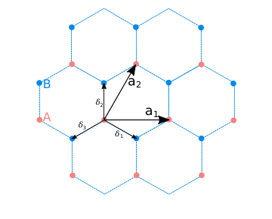
Figure 1: The honeycomb lattice of graphene with lattice parameter $\left|\boldsymbol{\delta}_{2}\right|=a_{0}$ and the armchair in the $\hat{y}$ direction. We have represented both the lattice vectors, ($\boldsymbol{a}_{1}$, $\boldsymbol{a}_{2}$), and the vectors connecting an A atom to its nearest neighbours, ($\boldsymbol{\delta}_{1}$, $\boldsymbol{\delta}_{2}$, $\boldsymbol{\delta}_{3}$). In plain graphene (PG), the atoms A and B are equivalent, in gapped graphene (GG), these are not.

III.2 Choosing a representation for the tight-binding Hamiltonian

There is a second issue concerning tight-binding Hamiltonians that, though it does not pertain solely to the velocity gauge, is extremely relevant in the calculation of nonlinear optical conductivities. For simplicity, we present the following discussion in terms of the nearest neighbour tight-binding model for the PG monolayer, since it will be used in our description of the nonlinear optical responses. The hopping parameter is set to $3$ eV, both in this section and throughout the rest of the work (Passos et al., 2018; Hipolito et al., 2018).

This Hamiltonian is usually written in two different ways,

$$H_{\mathbf{k},(a/\delta)}= \left[\begin{array}[]{cc}0&(-t)\ \phi_{(\delta/a)}(\mathbf{k})\\ (-t)\ \phi_{(\delta/a)}^{*}(\mathbf{k})&0\end{array}\right].$$ (37)

The first comes directly from the definition of the second Bloch basis as that in Eq.(27),

$$\phi_{(\delta)}(\mathbf{k})= \ e^{-i\mathbf{k}\cdot\boldsymbol{\delta}_{1}}+e^{-i\mathbf{k}\cdot\boldsymbol{\delta}_{2}}+e^{-i\mathbf{k}\cdot\boldsymbol{\delta}_{3}},$$ (38)

and is expressed in terms of the vectors connecting an atom to its nearest neighbours, Figure 1. The other way of writing this Hamiltonian is associated to a second Bloch basis that has its states phase shifted with respect to those of Eq.(27),

$$\bigl{|}\tilde{\psi}_{\mathbf{k}i}\bigr{\rangle}= \sum_{\mathbf{R}_{n}}e^{i\mathbf{k}\cdot\mathbf{R}_{n}}\bigl{|}\phi_{\mathbf{R}_{n}\,i}\bigr{\rangle},$$ (39)

such that hoppings are written in terms of the lattice vectors $\mathbf{a}_{1}$ and $\mathbf{a}_{2}$, (Cheng et al., 2014; Mikhailov, 2016; Passos et al., 2018),

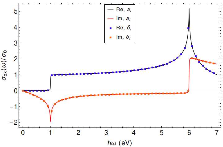
Figure 2: The real and imaginary parts of the interband portion of the linear conductivity, $\sigma_{xx}(\omega)$, for tight-binding Hamiltonians written in the lattice vector ($a_{i}$) and nearest neighbour ($\delta_{i}$) representations. The relevant parameters here are $\mu=0.5$ eV, $\gamma=0.005$ eV and $T=1$ K. The conductivity is normalized with respect to $\sigma_{0}=e^{2}/4\hbar$.

$$\phi_{(a)}(\mathbf{k})= \ 1+e^{i\mathbf{k}\cdot(\mathbf{a}_{2}-\mathbf{a}_{1})}+e^{i\mathbf{k}\cdot\mathbf{a}_{2}}.$$ (40)

Both representations have the same eigenvalues since the $\phi$ functions are related by a phase factor,

$$\phi_{(a)}(\mathbf{k})=e^{i\mathbf{k}\cdot\boldsymbol{\delta}_{2}}\,\phi_{(\delta)}(\mathbf{k}).$$ (41)

There is, however, a very important subtlety. If we use Eq.(31) to define the $h$ coefficients, or Eq.(34) to compute the Berry connection we obtain different results, both found in the literature, in the two representations: Eqs.(38) and (40).

It would appear that the condition for a trivial Berry connection in the entire FBZ, Eq.(29), that follows from the definition of the position operator of Eq.(28) is satisfied in the $\psi_{\mathbf{k}i}$ basis but it is not satisfied in the $\tilde{\psi}_{\mathbf{k}i}$ basis, since

$$\bigl{|}\tilde{u}_{\mathbf{k}i}\bigr{\rangle}=e^{-i\mathbf{k}\cdot\mathbf{r}}\bigl{|}\tilde{\psi}_{\mathbf{k}i}\bigr{\rangle}=\sum_{\mathbf{R}_{n}}e^{-i\mathbf{k}\cdot\boldsymbol{\delta}_{i}}\bigl{|}\phi_{\mathbf{R}_{n}\,i}\bigr{\rangle}$$ (42)

Still one needs to point out Eqs.(31) and (34) are still valid for the $\bigl{|}\tilde{\psi}_{\mathbf{k}i}\bigr{\rangle}$ basis of Eq.(39), provided we define $\mathbf{r}$ differently, effectively neglecting the distances inside the unit cell, $\left|\boldsymbol{\lambda}_{i}\right|$,

$$\mathbf{r}\bigl{|}\phi_{\mathbf{R}_{n}\,i}\bigr{\rangle}=\mathbf{R}_{n}\bigl{|}\phi_{\mathbf{R}_{n}\,i}\bigr{\rangle}.$$ (43)

These two different representations of the position operator, correspond naturally to different approximations to the perturbation term, and can lead to different results. To illustrate these distinctions it is worthwhile to compare the responses that follow from either representation, under the consideration that $h$ coefficients can be computed following Eq.(31), for both the zig-zag and armchair directions.

First, we consider the linear response along the zig-zag direction, $\sigma_{xx}(\omega)$, represented in Figure 2.

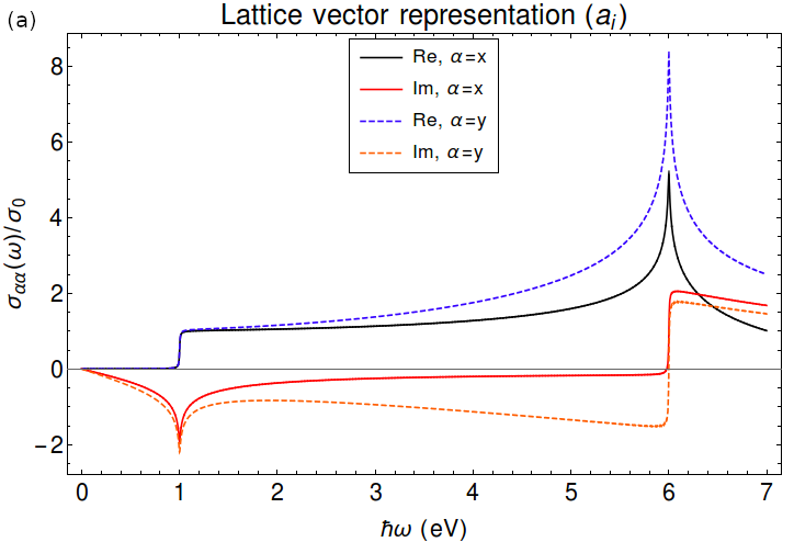
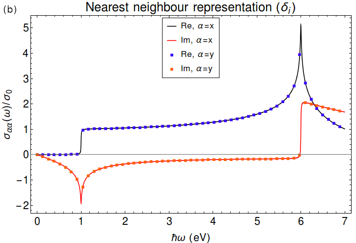
Figure 3: The real and imaginary parts of interband portion of the linear conductivities, $\sigma_{xx}(\omega)$ and $\sigma_{yy}(\omega)$, following from Eq.(40)/(38), the lattice vector representation (a) and the nearest neighbour representation (b). The chemical potential is again fixed to $0.5$ eV.

In this case, the responses that follow from the two representations are exactly the same, as both $\xi_{\mathbf{k}ij}^{x}$ and $\tilde{\xi}_{\mathbf{k}ij}^{x}$ are zero. This is due to the fact that $\boldsymbol{\delta}_{2}$ points in the $\hat{y}$ or armchair direction and as such, does not bear an influence in the response along the zig-zag direction. For the armchair direction, however, it is clear that the results in the two representations are different, Figure 3. More importantly, we can see that in lattice vector representation, the responses along zig-zag, $\sigma_{xx}(\omega)$, and armchair directions, $\sigma_{yy}(\omega)$, are different from one another, Figure 3(a). The use of the approximation described in Eq.(43) fails to properly translate the symmetry properties of the PG monolayer, particularly at high frequencies (Boyd, 2008). In the nearest neighbours representation, that property is indeed fulfilled. It was this latter representation that we used for the remaining numerical results in this work.

IV Results

In this section, we present the results for the second order response, i.e. the second harmonic generation and optical rectification conductivities, of the gapped graphene monolayer and for the third order response, i.e. the third harmonic generation and Kerr effect conductivities, of the plain and gapped monolayers to a monochromatic electric field. We considered different values for the gap and chemical potential, $\Delta$ and $\mu$, as well as different values for the scattering rate, $\gamma$, but not different values for the temperature, $T$, as its effect is similar to that of $\gamma$, which is to broaden the features. $T$ is thus set, throughout this work, to $1$K. Since all nonlinear optical conductivities are monotonically decreasing — the exception being the regions around processes at the gap (or twice the chemical potential) and around the van Hove singularities — these were represented in the two frequency regions separately, so as to make the features more visible. It must be said of these high frequency results that they should be taken only as an indication of what the response should look like — they were calculated in the independent particle approximation and, as such, do not consider the effect of excitons (Chae et al., 2011; Mak et al., 2014). Finally, we emphasize that the following conductivities satisfy the property of intrinsic permutation symmetry (Boyd, 2008).

IV.1 SECOND ORDER RESPONSE OF THE GAPPED GRAPHENE MONOLAYER

A gap is introduced in the plain graphene Hamiltonian, Eq.(37), by adding to it a term that breaks the equivalence between the A and B atoms, $\text{diag}(\Delta/2,-\Delta/2)$, and thus the centrosymmetricity of the PG monolayer. The study of the remaining symmetries in the point group then tells us that there is only one relevant component for this conductivity tensor: $\sigma_{yyy}$, with $y$ being the armchair direction (Hipolito et al., 2016). In addition, the relation between this component and the remaining nontrivial components reads as,

$$\sigma_{xxy}=\sigma_{xyx}=\sigma_{yxx}=-\sigma_{yyy}.$$ (44)

The following results have been normalized with respect to $\sigma_{2}=e^{3}a_{0}/4t\hbar=2.87\times 10^{-15}\text{ S$\cdot$m/V}$ (Hipolito et al., 2016).

IV.1.1 Second Harmonic Generation (SHG)

We begin with the study of the one photon ($\hbar\omega\sim\Delta$) and two photon ($2\hbar\omega\sim\Delta$) processes at the gap for values of $\Delta=30,\,300$ meV (Hipolito et al., 2018) and for two different values of the scattering rate, $\gamma=0.005,\,0.001$ eV, Figure 4.

   

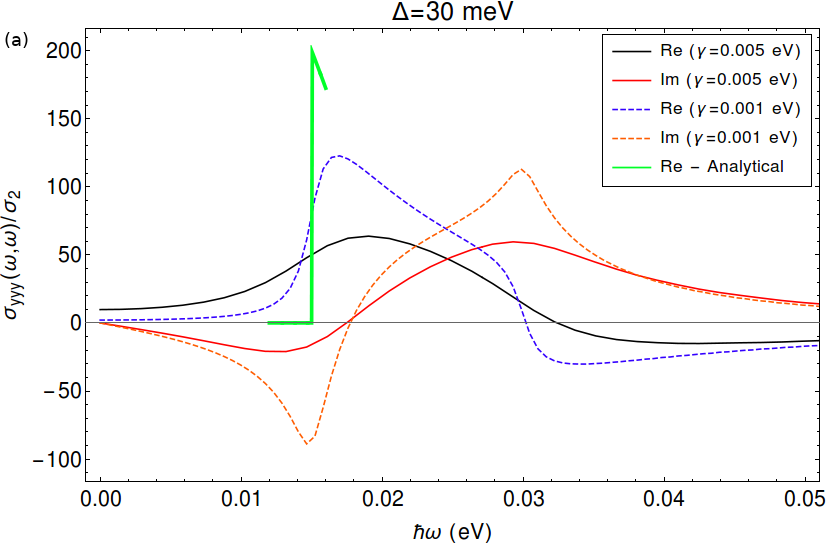
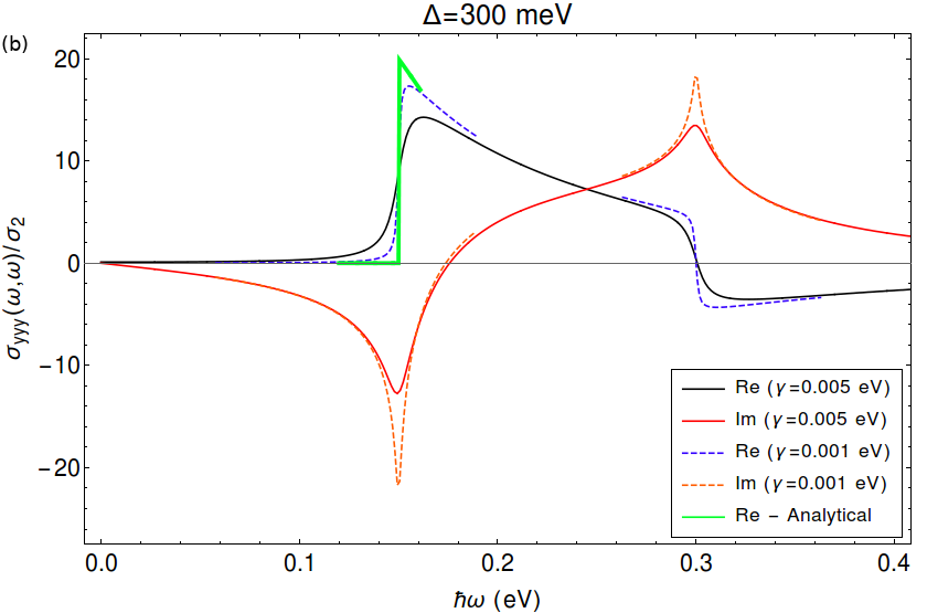
Figure 4: The real and imaginary parts of the second harmonic generation, $\sigma_{yyy}(\omega,\omega)$, close to the one photon and two photon processes at the gap: $30$ meV in the top plot, (a), and $\Delta=300$ meV in the bottom plot, (b) for different values of the scattering rate. The green curve represents the $\gamma=0$ analytical result. The parameters not listed in the plots are the chemical potential and the temperature, which will be fixed to $\mu=0$ eV, $T=1$K. These values are used in the remaining figures of this section.

It is clear from these results that the shape of the features is highly dependent on the interplay between the gap and scattering parameters, $\gamma$ and $\Delta$. For the larger scattering rate and smaller gap, we can see an overlap of the two and one photon peaks, Figure 4(a), which is markedly different from what happens for the larger gap, Figure 4(b), where the two peaks are clearly distinct. For smaller values of the scattering rate, represented by dashed curves, there is a sharpening of the features — now narrower and taller — and the results for the two gaps are similar. To study the zero scattering limit, $\gamma=0$, we turn to the analytical results — represented by the thicker green curve — that are obtained in the length gauge, Eq.(23). It can be shown that the real part of the two photon process in the second harmonic generation can be expressed in terms of the shift current coefficient that has been previously derived in (Aversa and Sipe, 1995; Sipe and Shkrebtii, 2000),

$$\frac{\text{Re}\left[\sigma_{yyy}(\omega,\omega)\right]}{\sigma_{2}}= -\frac{8it}{\pi}\int d^{2}\mathbf{k}\,\xi_{vc}^{y}\bigl{(}\xi_{cv}^{y}\bigr{)}_{;y}\ \delta(2\hbar\omega-\Delta\epsilon_{cv}).$$ (45)

using the standard notation for the generalized derivative, $\bigl{(}\xi_{ss^{\prime}}^{\alpha_{1}}\bigr{)}_{;\alpha_{2}}=\nabla_{\mathbf{k}}^{\alpha_{1}}(\xi_{ss^{\prime}}^{\alpha_{2}})-i(\xi_{ss}^{\alpha_{1}}-\xi_{s^{\prime}s^{\prime}}^{\alpha_{1}})\xi_{ss^{\prime}}^{\alpha_{2}}$ (Aversa and Sipe, 1995). By having a delta function in the integrand, one can see that the relevant contributions to the study of the two photon processes at the gap will come from the two regions of the FBZ around the band minimum, $\mathbf{K},\,\mathbf{K}^{\prime}=\pm 4\pi/3\sqrt{3}a_{0}\,\hat{x}$, which motivates a momentum expansion of the band around those points. Furthermore, since the delta function fixes $\Delta\epsilon_{cv}$ directly to twice the photon energy it is the suitable variable of integration,

$$\Delta\epsilon_{cv}^{2}= \Delta^{2}+4t^{2}\left|\phi_{\delta}(\mathbf{k})\right|^{2}.$$ (46)

Now, by expanding the hopping function, $\phi_{\delta}$, for small momenta around one of the band minima,

$$\left|\phi_{\delta}(\mathbf{k}=\mathbf{K}+\mathbf{q})\right|= \frac{3\left|\mathbf{q}\right|}{2}-\frac{3\left|\mathbf{q}\right|^{2}}{8}\text{cos}(3\theta)+\mathcal{O}(\left|\mathbf{q}\right|^{3}),$$ (47)

where $\left|\mathbf{q}\right|$ and $\theta$ are the radial and polar coordiantes associated with $\mathbf{q}$, and by rewriting Eq.(46) with the help of Eq.(47), we obtain,

$$\frac{1}{t}\sqrt{\Delta\epsilon_{cv}^{2}-\Delta^{2}}= \frac{3\left|\mathbf{q}\right|}{2}-\frac{3\left|\mathbf{q}\right|^{2}}{8}\text{cos}(3\theta)+\mathcal{O}(\left|\mathbf{q}\right|^{3}).$$ (48)

We have effectively related one of our integration variables, $\left|\mathbf{q}\right|$, with the small parameter $\delta(\Delta\epsilon_{cv})=\sqrt{\Delta\epsilon_{cv}^{2}-\Delta^{2}}/t$. It is now possible to invert this series, so as to obtain $\left|\mathbf{q}\right|$ in terms of $\delta$,

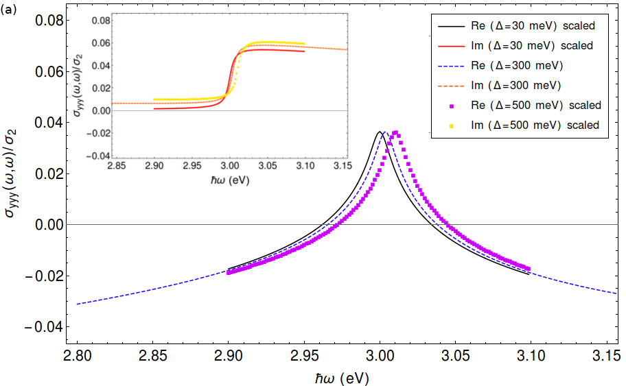
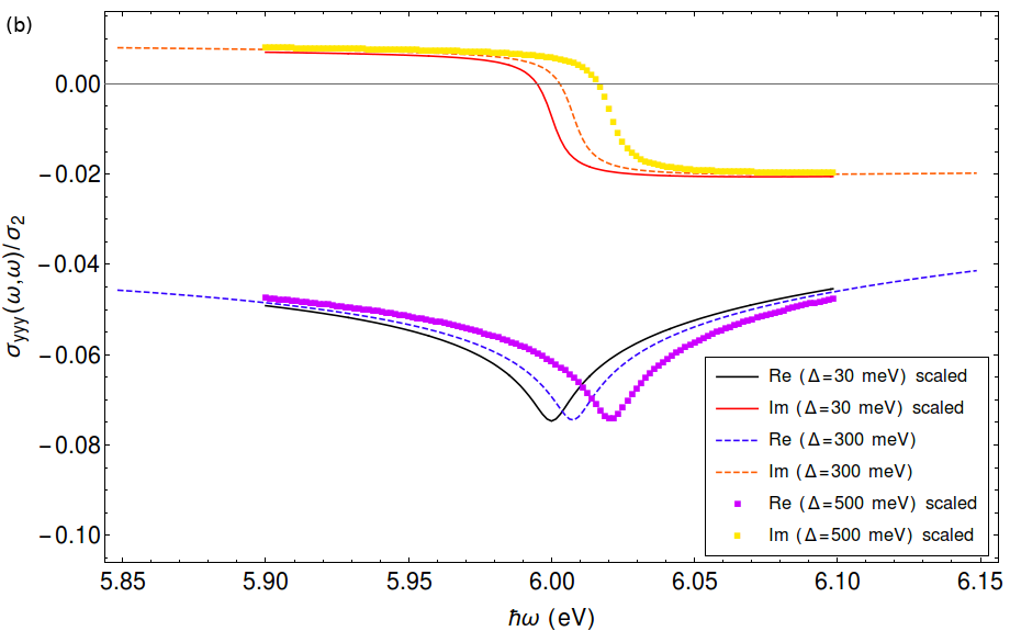
Figure 5: The real and imaginary parts of the SHG in GG, $\sigma_{yyy}(\omega,\omega)$, for frequencies around the two ($\hbar\omega\sim t$) (a) and one ($\hbar\omega\sim 2t$) (b) photon processes at the van Hove singularity. The imaginary parts for the two photon processes are represented on the inset. Curves labelled as scaled have been divided by a factor of $\Delta/300$ meV. The scattering parameter for these plots is $\gamma=0.005$ eV.

$$\left|\mathbf{q}\right| =\frac{\delta}{3}+\frac{\delta^{2}}{36}\text{cos}(3\theta)+\mathcal{O}(\delta^{3}).$$ (49)

Performing this change of variable in the integral, $\left|\mathbf{q}\right|\rightarrow\delta$, enables us to compute the integration in Eq.(45) analytically. The result is an expansion in powers of $(2\hbar\omega)^{2}-\Delta^{2}$, which in the lowest orders reads,

$$\frac{\text{Re}\left[\sigma_{yyy}(\omega,\omega)\right]}{\sigma_{2}}=\ \Theta(2\hbar\omega-\Delta)\Bigl{[}\frac{2t}{\Delta}+\Bigl{(}\frac{t}{9\Delta}-\frac{2t^{3}}{\Delta^{3}}\Bigr{)}$$

$$\times\Bigl{(}\Bigl{(}\frac{2\hbar\omega}{t}\Bigr{)}^{2}-\Bigl{(}\frac{\Delta}{t}\Bigr{)}^{2}\Bigr{)}+(...)\Bigr{]}.$$ (50)

This represented in Figure 4, alongside the numerical results of the velocity gauge. We must note that, had we carried only linear terms in $\left|\mathbf{q}\right|$ in the expansion of the hopping function, the $\text{Re}\left[\sigma_{yyy}(\omega,\omega)\right]$ would be exactly zero, for the same reason it vanishes in the monolayer of plain graphene: in that case, the Berry connections, $\xi_{\mathbf{q}ss^{\prime}}^{\alpha}$, are odd under $\mathbf{q}\rightarrow-\mathbf{q}$, and the integral vanishes necessarily. To obtain a nontrivial second order response in GG one has to consider the trigonal warping terms in the expansion of Eq.(47). The high frequency results, i.e. those for the two ($\hbar\omega\sim t$) and one ($\hbar\omega\sim 2t$) photon processes at the van Hove singularities, are represented in Figure 5. We can see that the features — for different values of $\Delta$ — are centered around slightly different different energies, as

$$\Delta\epsilon_{\textsc{vHs}}^{2}= \Delta^{2}+4t^{2}\left|\phi_{\delta}(\mathbf{M})\right|^{2}.$$ (51)

Note also that the absolute value of these conductivities scales with $\Delta$ — the opposite behavior to what we found for the response at the gap. Another, quite surprising, point concerns the features for the real and imaginary parts of these conductivities as they are switched with respect to the real and imaginary parts of the conductivities at the gap, Figure 4. It is now the real part that has the shape of a logarithmic-like divergence while the step-like behavior is present in the imaginary part.

IV.1.2 Optical Rectification

The other second order process that can be observed in the response to an external monochromatic field is the generation of a DC current, described by the optical recitification conductivity: $\sigma_{yyy}(\omega,-\omega)$, Figures 6 and 7.

From the inspection of the response at photon energies close to the value of the gap, $\hbar\omega\sim\Delta$, Figure 6, we can see that this tensor component is always finite (even in the zero scattering limit), meaning that there is indeed the absence of the injection current, as prescribed by the symmetry properties of the GG monolayer, Eq.(44). The remaining portion of this response is associated to the shift current and has a feature which is similar to that of the second harmonic generation at the gap, Figure 4(b). In the zero scattering limit, we have (Sipe and Shkrebtii, 2000),

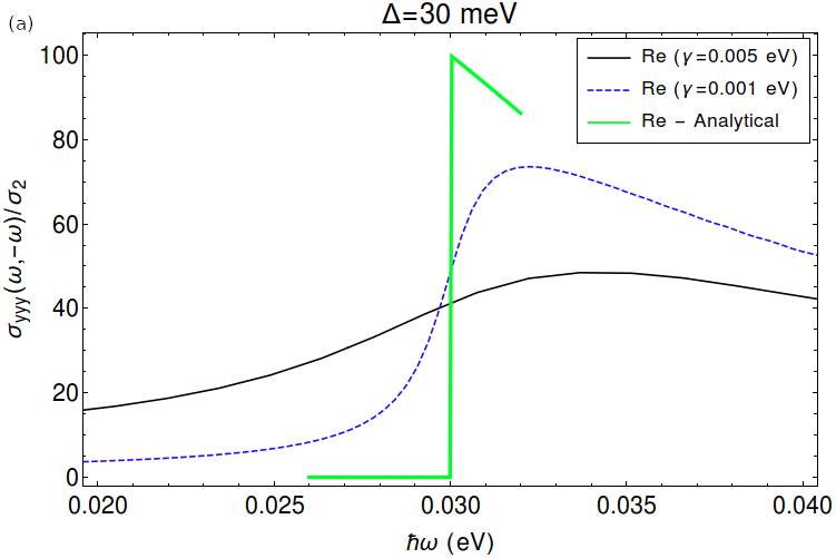
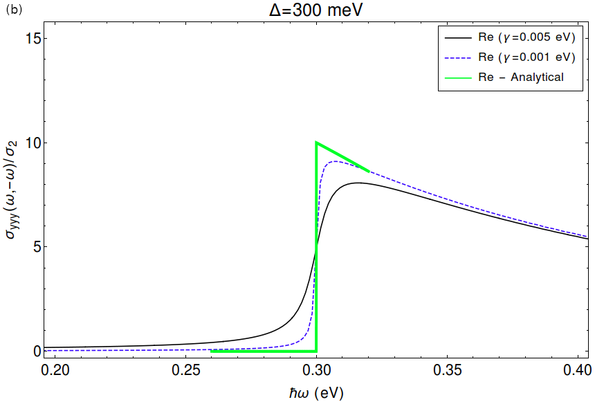
Figure 6: The optical rectification conductivity, $\sigma_{yyy}(\omega,-\omega)$, in GG for frequencies close to the gap: $\Delta=30$ meV in the top plot (a) and $\Delta=300$ meV in the bottom plot (b) for different values of the scattering rate. The green curve represents the $\gamma=0$ analytical result of Eq.(53).

$$\frac{\sigma_{yyy}(\omega,-\omega)}{\sigma_{2}}= -\frac{4it}{\pi}\int d^{2}\mathbf{k}\,\xi_{vc}^{y}\bigl{(}\xi_{cv}^{y}\bigr{)}_{;y}\ \delta(\hbar\omega-\Delta\epsilon_{cv}).$$ (52)

By comparison with the two photon resonance in the second harmonic generation, Eq.(50), we can see the two effects are essentially described by the same function with just different arguments — $2\omega$ in the case of the SHG — and an extra factor of two,

$$\frac{\text{Re}\left[\sigma_{yyy}(\omega,-\omega)\right]}{\sigma_{2}}=\ \Theta(\hbar\omega-\Delta)\Bigl{[}\frac{t}{\Delta}+\Bigl{(}\frac{t}{18\Delta}-\frac{t^{3}}{\Delta^{3}}\Bigr{)}$$

$$\times\Bigl{(}\Bigl{(}\frac{\hbar\omega}{t}\Bigr{)}^{2}-\Bigl{(}\frac{\Delta}{t}\Bigr{)}^{2}\Bigr{)}+(...)\Bigr{]}.$$ (53)

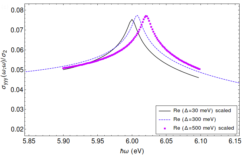
Figure 7: The optical rectification conductivity, $\sigma_{yyy}(\omega,-\omega)$, in GG for frequencies around the one photon process at the van Hove singularity. Curves labelled as scaled have been divided by a factor of $\Delta/300$ meV. The scattering parameter in this plot is $\gamma=0.005$ eV.

The similarity between the optical rectification conductivity and the second harmonic generation is also present at higher frequencies, $\hbar\omega\sim 2t$, Figure 7. Apart from a sign switch and the absence of the imaginary part — the symmetrized optical rectification conductivity is necessarily real — this result is very similar that of Figure 5(b).

IV.2 THIRD ORDER RESPONSE OF THE GG AND PG MONOLAYERS

The third order response is finite even in the presence of inversion symmetry and as such, we present results for both the gapped graphene and the plain graphene monolayers for the nonlinear processes of third harmonic generation and optical Kerr effect. Though associated to different point group symmetries, the components of their third order conductivities satisfy the same relations,

$$\begin{array}[]{c}\sigma_{yyyy}=\sigma_{xxxx}=\sigma_{xxyy}+\sigma_{xyxy}+\sigma_{xyyx},\\ \sigma_{xxyy}=\sigma_{yyxx},\ \sigma_{xyxy}=\sigma_{yxyx},\ \sigma_{xyyx}=\sigma_{yxxy}.\end{array}$$ (54)

As we are also imposing intrinsic permutation symmetry, there is only one relevant component in third harmonic generation (THG), with all other components of the tensor trivially expressed in terms of it,

$$\begin{array}[]{c}\sigma_{xxyy}(\omega,\omega,\omega)=\sigma_{xyxy}(\omega,\omega,\omega)=\sigma_{xyyx}(\omega,\omega,\omega),\\ \sigma_{xxyy}(\omega,\omega,\omega)=\frac{1}{3}\sigma_{xxxx}(\omega,\omega,\omega)=\frac{1}{3}\sigma_{yyyy}(\omega,\omega,\omega).\end{array}$$ (55)

We will thus present only the $\sigma_{yyyy}$ in our study of the THG. For the optical Kerr effect, we consider both the $\sigma_{yyyy}$ and $\sigma_{yxxy}$ components. The following results have been normalized by $\sigma_{3}=e^{4}a_{0}^{2}/8\hbar t^{2}=6.84\times 10^{-26}\text{ S$\cdot$m}^{2}\text{/V}^{2}$.

IV.2.1 Third Harmonic Generation (THG)

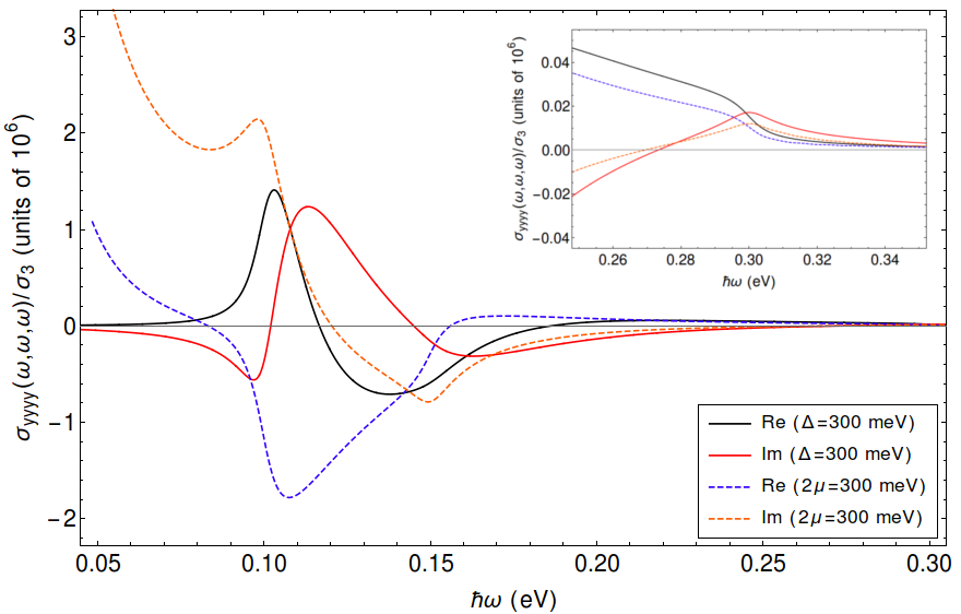
Figure 8: The real and imaginary parts of the third harmonic generation, $\sigma_{yyyy}(\omega,\omega,\omega)$, in the GG, $\Delta=300$ meV, and PG, $2\mu=300$ meV, monolayers for frequencies that cover the different (one, two and three) photon processes at the gap / twice the value of the chemical potential. Note that the vertical scale is in units of $10^{6}$. The inset represents a zoom-in in the region of the one photon process, $\hbar\omega\sim\Delta,\,2\mu$.

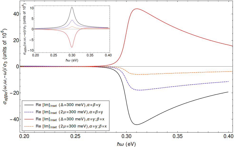
Figure 9: The real and imaginary parts (the latter is represented in the inset) of the optical Kerr effect for the components, $\sigma_{yyyy}(\omega,\omega,-\omega)$ and $\sigma_{yxxy}(\omega,\omega,-\omega)$, in the GG, $\Delta=300$ meV, and PG, $2\mu=300$ meV, monolayers for frequencies around the one photon process at the gap / twice the value of the chemical potential. Note that the vertical scale is in units of $10^{6}$.

One of the points covered in a previous subsection (SHG) concerned the interplay between $\Delta$ and $\gamma$, and how this affected the features one sees in the conductivities. If one were to do this analysis in the THG, one would again conclude that for larger scattering rates one sees a broadening, possibly even a merger, of the main features in the conductivity. The scattering rate is therefore fixed to $\gamma=0.005$ eV. We will, instead, focus on the THG of the gapped and plain graphene monolayers, in the case where the value of the gap in the GG is equal to the energy value of the region of states that are Pauli-blocked, $2\mu$, of the PG, and that this is equal to $300$ meV, Figures 8 and 10.

We begin by studying the response of the several different photon processes, $n\hbar\omega=\Delta,\,2\mu$ for $n=1,2,3$, Figure 8. It is clear that the conductivities for gapped and plain graphene are very much different: for the three photon resonance, there are prominent features in both sets of curves but the sign appears to be switched with respect to one another; for the two photon resonance, there are no clear features in the GG monolayer, whereas in the PG, one finds a shoulder and a local minimum in the real and imaginary parts, respectively. An exception to this, however, are the features for the one photon process, inset of Figure 8. The differences between the low frequency limit of the gapped and plain graphene monolayer can be easily ascribed to the intraband terms of the response, dominant in this frequency range, that are completely absent from the response of the GG — a cold semiconductor — but present in the response of the doped PG monolayer.

For higher frequencies, associated with the different processes around the van Hove singularities, Figure 10, we can see that the conductivities of the PG and GG monolayers are rather similar. For those energies, the band structures are rather similar (as $\Delta\ll t$) and the chemical potential that is set in the PG is completely irrelevant. The only difference in the two curves comes from the different energy values for the van Hove singularity, Eq.(51).

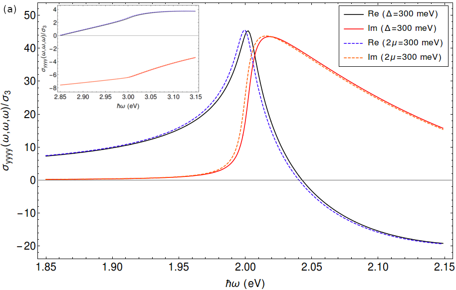
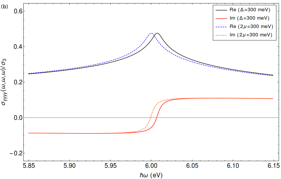
Figure 10: The real and imaginary parts of the third harmonic generation, $\sigma_{yyyy}(\omega,\omega,\omega)$, for frequencies around the three photon ($3\hbar\omega\sim 2t$), (a), two photon ($\hbar\omega\sim t$), inset of (a), and one photon ($\hbar\omega\sim 2t$), (b), processes at the van Hove singularity in the GG, $\Delta=300$ meV, and PG, $2\mu=300$ meV, monolayers.

      

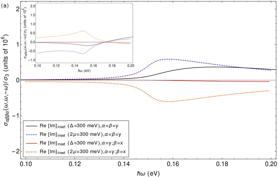
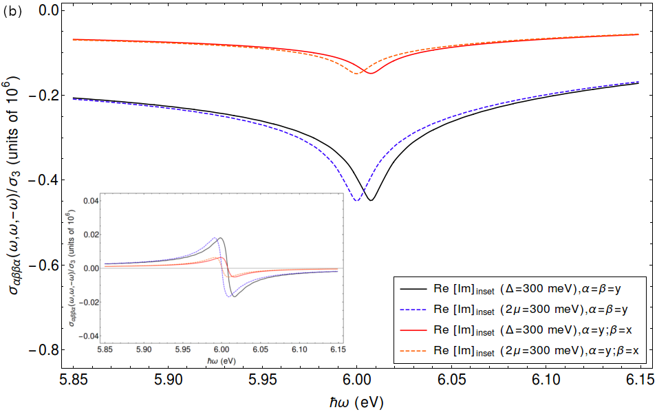
Figure 11: The real and imaginary (the latter represented in the insets) parts of the Kerr effect, $\sigma_{yyyy}(\omega,\omega,-\omega)$, in the GG, $\Delta=300$ meV, and PG, $2\mu=300$ meV, monolayers for frequencies around $\Delta=\,2\mu$, (a), and for frequencies around the van Hove singularity, (b). Note that the vertical scale in both figures is in units of $10^{6}$.

      

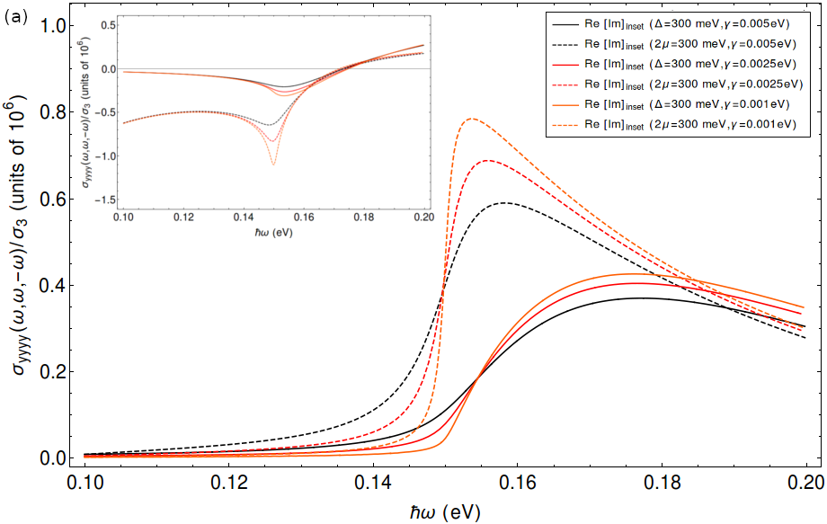
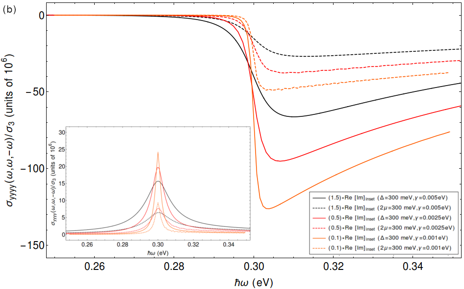
Figure 12: The real and imaginary (the latter represented in the insets) parts of the Kerr effect, $\sigma_{yyyy}(\omega,\omega,-\omega)$, in the GG, $\Delta=300$ meV, and PG, $2\mu=300$ meV, monolayers for frequencies around $2\hbar\omega\sim\Delta=\,2\mu$ (a), and for frequencies around $\hbar\omega\sim\Delta=\,2\mu$ (b) for different values of the scattering parameter: $\gamma=0.005$ eV (black), $\gamma=0.0025$ eV (red) and $\gamma=0.001$ eV (orange). Note that in (b), the conductivities for different $\gamma$ have been scaled by different factors: $1.5$ for black, $0.5$ for red and $0.1$ for orange. As before, the vertical scale in both figures is in units of $10^{6}$.

IV.2.2 Optical Kerr Effect (OKE)

Our final set of results concerns the optical Kerr effect (OKE), once again calculated for the cases of the GG and PG monolayers of parameters, $\Delta=2\mu$. Now, unlike the THG — Eq.(55) — not all nonzero components of the conductivity tensor associated with the OKE can be directly related to the diagonal terms. To show their differences, we present the $\sigma_{yyyy}(\omega,\omega,-\omega)$ and $\sigma_{yxxy}(\omega,\omega,-\omega)$ components in the low-frequency portion of the response, i.e. around the one and two photon processes at the gap (twice the chemical potential for the PG), Figures 9 and 11(a), as well as the response around the one photon process at the van Hove singularity, Figure (11)(b). Figure 9 shows that the two conductivity components of the GG monolayer have opposite signs — in both the real and the imaginary part — and that they are similar, but not exactly equal, in modulus. In the PG, it is only the height of the features that is different, being less pronouced in the off-diagonal component. For the two photon processes at the gap (twice the chemical potential), Figure 11(a), both the GG and PG conductivities display sign differences between the two tensor components and the property observed in the one photon seems to appear in reverse: here it is in the response of the GG that we see the less pronounced features for the off-diagonal component; the PG conductivities have opposite signs and are rather similar, in modulus, across the frequency range considered. For the high frequency response, i.e. one photon processes at the van Hove singularity, Figure 11(b), we see that the features on both components of the OKE conductivity are essentially the same, differing only by an overall factor of three. As in the THG, the only distinction between responses of the GG and PG monolayers comes from the fact the different energy values for the van Hove singularity: slightly higher in the GG monolayer, Eq.(51).

A second point of interest in the OKE concerns the existence of a divergence in the real part of its associated conductivity for frequencies above the one photon absorption at the gap (twice the chemical potential) in the scatteringless limit (Aversa and Sipe, 1995), that is related to the acceleration of electron-hole pairs — produced in one photon absorption processes — by a static, nonlinear, electric field. This divergence should be present in both the GG and PG monolayers and was indeed seen in an analytical calculation of the OKE in the monolayer of plain graphene, in the context of a linearized band (Cheng et al., 2014). Although we cannot probe this singularity directly — in the sense that the scattering parameter is necessarily finite in the numerical calculations — we find that it is nonetheless clear that such a divergence does exists, in both the PG and the GG monolayer. Figure (12) represents the real and imaginary parts of the OKE conductivity for frequencies around the two photon (a) and one photon (b) at the gap (twice the chemical potential) for different values of the scattering parameter, $\gamma$. For frequencies, $2\hbar\omega\sim\Delta=2\mu$, Figure (12)(a), we can see that a decrease in the value of $\gamma$ is associated with sharper features in a small region around the absorption threshold, that then tend to merge as one moves to frequencies away from those around the threshold. This is similar to what we have observed in Figures 4(b) and 6(b) and it is the expected behavior for features in any given regular conductivity. When we move to frequencies above the one photon absorption, $\hbar\omega\geq\Delta=2\mu$, this no longer holds for the real part of the OKE conductivity. It increases in absolute value as $\gamma$ is reduced with the curves for different $\gamma$ running parallel to one another. Instead of a well-localized feature, one can see the appearance of a divergence.

V SUMMARY

In this work we have studied second and third harmonic generation, the optical rectification and the optical Kerr effect for the gapped and plain graphene monolayers to a monochromatic pulse by using the density matrix formalism in the velocity gauge as well as in the length gauge. Although the topic is not new, this is the first work to present all tensor components of the nonlinear conductivities of these materials, in a frequency range that extends beyond the Dirac approximation. We emphasize that the tensor components considered here are not the effective tensors of ref.(Hipolito et al., 2018), the use of which, we think, has not been adequately justified.

To calculate the conductivities in this work, we used the velocity gauge formalism developed in a previous work (Passos et al., 2018) with an additional point that we presented here: the choice of an adequate basis — the second Bloch basis — can be used to reduce covariant derivatives to regular k-space derivatives, which in turn simplifies the computation of the $h$ coefficients that are required for the calculation of nonlinear optical responses in the velocity gauge. We have also shown how this treatment of the covariant derivative is related to the representation of the position operator, the choice of which bears an influence in the results.

As for the nonlinear conductivities themselves: for the second harmonic generation and the optical rectification conductivity at the gap, the numerical results of the velocity gauge were complemented by analytical, zero scattering limit, results in the length gauge. From these numerical results we saw how the interplay between the gap, $\Delta$, and the scattering rate, $\gamma$, affected the form of the features at low frequency. For higher frequencies, that is, around the van Hove singularity, we saw the relation between conductivities of GG monolayers with different values of the gap as well as a blueshift of the features for increasing values of $\Delta$. For the third order response, we instead focused on a comparison between the responses of the gapped graphene and doped plain graphene monolayer, in the case where the excluded energy region for interband transitions is the same, i.e., $\Delta=2\mu$. We saw, in the case of the THG, that the low frequency limit in the two materials is very different, which can be traced back to the presence of intraband terms in the response of the doped PG monolayer. For higher frequencies, the two responses are very much alike, with the exception of the shift that follows from the different location of the van Hove singularity. For the OKE, we studied two different components of the conductivity tensor, for both low and high frequencies, as well as the existence of a divergence for frequencies above the one photon absorption at the gap (twice the chemical potential) in the response of both the PG and the GG monolayers.

The authors acknowledge financing of Fundação da Ciência e Tecnologia, of COMPETE 2020 program in FEDER component (European Union), through projects POCI-01-0145-FEDER-028887 and UID/FIS/04650/2013. G. B. V. would like to thank Emilia Ridolfi and Vítor M. Pereira of the Centre for Advanced 2D Materials at the National University of Singapore for useful discussions, Nuno M. R. Peres for his help reviewing the manuscript and Simão Meneses João for providing Figure 1.

References

- Mikhailov (2007) S. A. Mikhailov, EPL (Europhysics Letters) 79, 27002 (2007).
- Mikhailov and Ziegler (2008) S. A. Mikhailov and K. Ziegler, Journal of Physics: Condensed Matter 20, 384204 (2008).
- Al-Naib et al. (2014) I. Al-Naib, J. E. Sipe, and M. M. Dignam, Phys. Rev. B 90, 245423 (2014).
- Glazov and Ganichev (2014) M. M. Glazov and S. D. Ganichev, Physics Reports 535, 101 (2014).
- Peres et al. (2014) N. M. R. Peres, Y. V. Bludov, J. E. Santos, A.-P. Jauho, and M. I. Vasilevskiy, Phys. Rev. B 90, 125425 (2014).
- Cheng et al. (2014) J. L. Cheng, N. Vermeulen, and J. E. Sipe, New Journal of Physics 16, 053014 (2014).
- Cheng et al. (2015a) J. L. Cheng, N. Vermeulen, and J. E. Sipe, Phys. Rev. B 92, 235307 (2015a).
- Cheng et al. (2015b) J. L. Cheng, N. Vermeulen, and J. E. Sipe, Phys. Rev. B 91, 235320 (2015b).
- Mikhailov (2016) S. A. Mikhailov, Phys. Rev. B 93, 085403 (2016).
- Semnani et al. (2016) B. Semnani, A. H. Majedi, and S. Safavi-Naeini, Journal of Optics 18, 035402 (2016).
- Mikhailov (2017) S. A. Mikhailov, Phys. Rev. B 95, 085432 (2017).
- Savostianova and Mikhailov (2017) N. A. Savostianova and S. A. Mikhailov, Opt. Express 25, 3268 (2017).
- Ventura et al. (2017) G. B. Ventura, D. J. Passos, J. M. B. Lopes dos Santos, J. M. Viana Parente Lopes, and N. M. R. Peres, Phys. Rev. B 96, 035431 (2017).
- Passos et al. (2018) D. J. Passos, G. B. Ventura, J. M. V. P. Lopes, J. M. B. L. d. Santos, and N. M. R. Peres, Phys. Rev. B 97, 235446 (2018).
- Savostianova and Mikhailov (2018) N. A. Savostianova and S. A. Mikhailov, Phys. Rev. B 97, 165424 (2018).
- Hipolito et al. (2018) F. Hipolito, A. Taghizadeh, and T. G. Pedersen, Phys. Rev. B 98, 205420 (2018).
- Hendry et al. (2010) E. Hendry, P. J. Hale, J. Moger, A. K. Savchenko, and S. A. Mikhailov, Phys. Rev. Lett. 105, 097401 (2010).
- Dean and van Driel (2010) J. J. Dean and H. M. van Driel, Phys. Rev. B 82, 125411 (2010).
- Zhang et al. (2012) H. Zhang, S. Virally, Q. Bao, L. K. Ping, S. Massar, N. Godbout, and P. Kockaert, Opt. Lett. 37, 1856 (2012).
- Kumar et al. (2013) N. Kumar, J. Kumar, C. Gerstenkorn, R. Wang, H.-Y. Chiu, A. L. Smirl, and H. Zhao, Phys. Rev. B 87, 121406 (2013).
- Hong et al. (2013) S.-Y. Hong, J. I. Dadap, N. Petrone, P.-C. Yeh, J. Hone, and R. M. Osgood, Phys. Rev. X 3, 021014 (2013).
- Dremetsika et al. (2016) E. Dremetsika, B. Dlubak, S.-P. Gorza, C. Ciret, M.-B. Martin, S. Hofmann, P. Seneor, D. Dolfi, S. Massar, P. Emplit, and P. Kockaert, Opt. Lett. 41, 3281 (2016).
- Vermeulen et al. (2016) N. Vermeulen, D. Castelló-Lurbe, J. Cheng, I. Pasternak, A. Krajewska, T. Ciuk, W. Strupinski, H. Thienpont, and J. Van Erps, Phys. Rev. Applied 6, 044006 (2016).
- Higuchi et al. (2017) T. Higuchi, C. Heide, K. Ullmann, H. B. Weber, and P. Hommelhoff, Nature 550, 224 (2017).
- Baudisch et al. (2018) M. Baudisch, A. Marini, J. D. Cox, T. Zhu, F. Silva, S. Teichmann, M. Massicotte, F. Koppens, L. S. Levitov, F. J. Garcia de Abajo, and J. Biegert, Nature Communications 9, 1018 (2018).
- Janisch et al. (2014) C. Janisch, Y. Wang, D. Ma, N. Mehta, A. L. ElÃas, N. Perea-Lopez, M. Terrones, V. Crespi, and Z. Liu, Nature: Scientific Reports 4, 5530 (2014).
- Pedersen (2015) T. G. Pedersen, Phys. Rev. B 92, 235432 (2015).
- Hipolito et al. (2016) F. Hipolito, T. G. Pedersen, and V. M. Pereira, Phys. Rev. B 94, 045434 (2016).
- Hipolito and Pedersen (2018) F. Hipolito and T. G. Pedersen, Phys. Rev. B 97, 035431 (2018).
- Youngblood et al. (2017) N. Youngblood, R. Peng, A. Nemilentsau, T. Low, and M. Li, ACS Photonics 4, 8 (2017).
- Moss et al. (1989) D. J. Moss, E. Ghahramani, J. E. Sipe, and H. M. Van Driel, Phys. Rev. B 41, 15 (1989).
- Sipe and Ghahramani (1993) J. E. Sipe and E. Ghahramani, Phys. Rev. B 48, 11705 (1993).
- Aversa and Sipe (1995) C. Aversa and J. E. Sipe, Phys. Rev. B 52, 14636 (1995).
- Sipe and Shkrebtii (2000) J. Sipe and A. Shkrebtii, Phys. Rev. B 61, 5337 (2000).
- Parker et al. (2019) D. E. Parker, T. Morimoto, J. Orenstein, and J. E. Moore, Phys. Rev. B 99, 045121 (2019).
- João and Lopes (2018) S. M. João and J. M. V. P. Lopes, arXiv e-prints , arXiv:1810.03732 (2018), arXiv:1810.03732 [cond-mat.other] .
- Boyd (2008) R. W. Boyd, Nonlinear Optics, Third Edition, 3rd ed. (Academic Press, 2008).
- Note (1) We consider two things in the following expressions: repeated cartesian indexes are being implicitly summed over; conductivities satisfy the property of intrinsic permutation symmetry (Boyd, 2008).
- Blount (1962) E. I. Blount, Solid State Physics: Advances in Research and Applications, edited by F. Seitz and D. Turnbull, Vol. 13 (Academic, New York, 1962).
- Chae et al. (2011) D.-H. Chae, T. Utikal, S. Weisenburger, H. Giessen, K. v. Klitzing, M. Lippitz, and J. Smet, Nano Letters 11, 1379 (2011), pMID: 21322607, https://doi.org/10.1021/nl200040q .
- Mak et al. (2014) K. F. Mak, F. H. da Jornada, K. He, J. Deslippe, N. Petrone, J. Hone, J. Shan, S. G. Louie, and T. F. Heinz, Phys. Rev. Lett. 112, 207401 (2014).
- Note (2) We have compared this with the analytical result of ref.(Hipolito et al., 2016) and found a minus sign discrepancy, which — according to our calculations — follows from excluding the derivative portion of the generalized derivative.