MorteX method for contact along real and embedded surfaces:
coupling X-FEM with the Mortar method

Abstract

A method to treat frictional contact problems along embedded surfaces in the finite element framework is developed. Arbitrarily shaped embedded surfaces, cutting through finite element meshes, are handled by the X-FEM. The frictional contact problem is solved using the monolithic augmented Lagrangian method within the mortar framework which was adapted for handling embedded surfaces. We report that the resulting mixed formulation is prone to mesh locking in case of high elastic and mesh density contrasts across the contact interface. The mesh locking manifests itself in spurious stress oscillations in the vicinity of the contact interface. We demonstrate that in the classical patch test, these oscillations can be removed simply by using triangular blending elements. In a more general case, the triangulation is shown inefficient, therefore stabilization of the problem is achieved by adopting a recently proposed coarse-graining interpolation of Lagrange multipliers. Moreover, we demonstrate that the coarse-graining is also beneficial for the classical mortar method to avoid spurious oscillations for contact interfaces with high elastic contrast. The performance of this novel method, called MorteX, is demonstrated on several examples which show as accurate treatment of frictional contact along embedded surfaces as the classical mortar method along boundary fitted surfaces.

1 Introduction

Among the wide spectrum of engineering applications, the class of problems involving contact interactions between solids are complex both with regard to their mathematical description and numerical treatment. The transfer of mechanical forces, thermal or electrical conduction, tectonic plate movements are merely a few examples of the ubiquity of contact in nature and engineering applications. The vast majority of phenomena occurring at the contact interface, such as wear, adhesion, lubrication and fretting, as well as mass and energy transfer, determine to the greater extent the service life of engineering components. This lays a strong emphasis on the importance to gain a fine understanding of these mechanisms for the accurate analysis and timely prediction of failure. In the last decade, a class of surface-to-surface contact discretizations, such as mortar method, coupled with appropriate treatment of inequality contact constraints has been well established and proved its ability to efficiently treat contact problems [47, 25, 43]. However, the numerical treatment of the contact and related phenomena remains particularly challenging when it involves the evolution of complex surfaces. These complexities can involve cumbersome remeshing algorithms and field transfer procedures, as for instance those encountered in the context of wear. In addition, construction of adequate finite element meshes near contact interfaces and stability of the contact formulations are necessary ingredients to ensure the overall efficiency, accuracy and robustness of the numerical procedures.

In this work, first we present a coherent framework for mortar frictional contact based on the monolithic augmented Lagrangian method for both normal and tangential contact components [2, 15]. We then extend this framework for a two dimensional unified framework, called MorteX, capable to treat frictional contact problems between a real and a virtual (intra-mesh) surfaces. It combines the features of Generalized/Extended Finite element methods (GFEM/X-FEM) [18, 9] and mortar methods for solving the contact problems [7, 37, 47, 44]. This unified framework was elaborated in [1] for mesh tying problems and is extended here to handle frictional contact problems. Within the proposed framework, in a discretized setting (see Fig. 1) the contact constraints are imposed between a “real” surface $\displaystyle\Gamma_{c}^{1}$ (explicitly represented by edges of finite elements) and an embedded virtual surfaces $\displaystyle\Gamma^{2}_{c}$ (internal surface geometrically non-conformal with the underlying discretization).

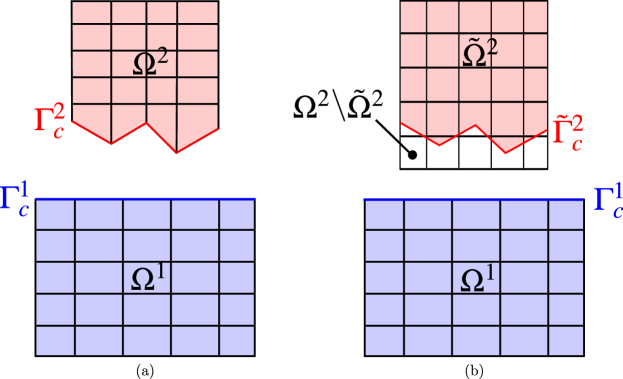
Figure 1: Equivalent discrete setting of two deformable bodies coming in contact: (a) the contact surfaces $\displaystyle\Gamma^{1}_{c}$ and $\displaystyle\Gamma^{2}_{c}$ are conformal to the boundaries of discretized solids; (b) contact boundary $\displaystyle\Gamma^{1}_{c}$ is still conformal, while the homologue deformable body is now $\displaystyle\tilde{\Omega}^{2}$ and its contact boundary $\displaystyle\tilde{\Gamma}^{2}_{c}$ is embeded in the domain $\displaystyle\Omega^{2}$, whose part $\displaystyle\Omega^{2}\setminus\tilde{\Omega}^{2}$ is discarded from the computation.

The X-FEM is an enrichment method based on the partition of unity (PUM) for discontinuous fields [38, 4]. In this framework, discontinuities are not explicitly modeled, and as a result, the mesh is not required to conform to these discontinuities. In X-FEM, enrichment functions are added to the finite element interpolation using the framework of PUM, to account for non-smooth behavior without compromising on the optimal convergence [22]. The X-FEM methods are extensively used in applications such as fracture mechanics, shock wave front and oxidation front propagation, and other applications involving discontinuities both strong and weak [52, 53, 16, 28, 32], and in particular for the contact between crack lips [17, 34, 49, 20, 36, 27, 40]. The ability of the X-FEM to describe geometric features (e.g. inclusions and voids) independently of the underlying mesh, will be exploited in the proposed unified framework to describe complex and evolving surfaces.

As opposed to the node-to-node discretisation which is limited to small sliding and the node-to-surface method which is inaccurate, the surface-to-surface based mortar methods are stable and very accurate in treating contact problems under finite sliding conditions [19]. The mortar methods provide us with a comprehensive framework to address the limitations of incompatible interface discretizations. They are a subclass of domain decomposition methods (DDM), that are tailored for non-conformal spatial interface discretizations [10], and were originally introduced for spectral elements [8, 11]. The coupling and tying of different physical models, discretization schemes, and/or non-matching discretizations along interfaces between the domains can be ensured by mortar methods. The mathematical optimality and applicability of the mortar methods in spectral and finite element frameworks were studied extensively for elliptic problems in [11, 8, 56]. The mortar methods were brought into the contact realm with the initial contributions from Belgacem et al., Hild, Laursen et al.  [7, 31, 37]. Subsequent works of Fischer and Wriggers  [24, 25], Puso and Laursen  [47, 46] have extended the application of mortar methods to the class of non-linear problems. The work of Popp, Gietterle, et al [26, 43] dealt with the class of dual Lagrangian resolution schemes  [55].

In the present methodology, we use the monolithic augmented Lagrange multiplier resolution scheme to treat the frictional contact problems. It represents a so-called mixed formulation [13]. The choice of Lagrange multipliers’ functional space strongly affects the convergence rate and can lead to loss of accuracy in the interfacial tractions. These difficulties arise from a locking type phenomena reported for mixed variational formulations as a result of non-satisfaction of Ladyzhenskaya-Babuška-Brezzi (LBB) [3, 13]. This locking, present in standard FEM with Lagrange multipliers on the boundary [5], but also in the mixed X-FEM framework when Dirichlet boundary conditions are applied along embedded surfaces, was extensively studied in [21, 39, 6, 14, 29, 48]. However, to the best of our knowledge, the manifestation of mesh locking effects when imposing contact constraints using Lagrange multipliers, was never reported. The manifestation of the locking effect will be illustrated in the present work for contact problems both in the context of standard mortar and MorteX methods. In addition, stabilization strategies initially proposed for the mesh tying problems in the context of MorteX method [1], are adapted here for contact applications.

The paper is organized as follows. In Section 2 and 3, we present the strong and weak continuum problem description of two-body frictional contact. The classical spatial mortar interface discretization scheme for the frictional contact problem is derived in Section 4. In Section 6 this framework is extended to account for embedded contact surfaces, and referred as MorteX framework. It will explicitly detail the features of the X-FEM and adaptation of the mortar which are needed to construct a coherent computational scheme. In Section 8, few examples including the contact patch test are considered to illustrate the methods performance for both frictionless and frictional contact problem settings. In Section 9, we give the concluding remarks and present the prospective works.

2 Problem definition

The case of two deformable bodies in contact is considered, for simplicity the derivations are made in infinitesimal deformation formalism, but is readily extandable to the finite strain framework. Fig. 2 shows two statements of this contact problem: (a) is a classical formulation where the solids come in contact over their outer surfaces. In (b) an equivalent, from continuum point of view, setting is shown, whereby contact boundary $\displaystyle\Gamma^{1}_{c}$ is still an outer boundary of $\displaystyle\Omega^{1}$, while the homologue deformable body is now $\displaystyle\tilde{\Omega}^{2}$ and its contact boundary $\displaystyle\tilde{\Gamma}^{2}_{c}$ is embeded in the domain $\displaystyle\Omega^{2}$, whose part $\displaystyle\Omega^{2}\setminus\tilde{\Omega}^{2}$ is discarded from the computation. In the current and next two sections, we will state the problem and suggest the methods to handle the configuration shown in Fig. 2(a), whereas in Section 6, we will extend these methods to deal with the problem shown in Fig. 2(b). The domains $\displaystyle\Omega^{i}$, $\displaystyle i=1,\,2$, have non-intersecting Dirichlet boundaries $\displaystyle\Gamma_{u}^{i}$, Neumann boundaries $\displaystyle\Gamma_{t}^{i}$ and contact boundaries $\displaystyle\Gamma_{c}^{i}$, i.e. $\displaystyle\partial{\Omega^{i}}=\Gamma_{u}^{i}\cup\Gamma_{t}^{i}\cup\Gamma_{c}^{i}$. The standard boundary value problem (BVP) is described by the balance of linear momentum along with the imposed boundary conditions:

$$\displaystyle\nabla\cdot\underline{\underline{\bm{\sigma}}}^{i}+\underline{\bm{f}}_{v}^{i} \displaystyle=0\quad\mbox{in}\,\,\Omega^{i},$$ (1)

$$\displaystyle\underline{\underline{\bm{\sigma}}}^{i}\cdot\underline{\bm{n}}^{i} \displaystyle=\underline{\bm{\hat{t}}}^{i}\quad\mbox{on}\,\,\Gamma_{t}^{i},$$ (2)

$$\displaystyle\underline{\bm{u}}^{i} \displaystyle=\underline{\bm{\hat{u}}}^{i}\quad\mbox{on}\,\,\Gamma_{u}^{i},$$ (3)

$$\displaystyle\underline{\underline{\bm{\sigma}}}^{i}\cdot\underline{\bm{n}}^{i} \displaystyle=\underline{\bm{t}}^{i}_{c}\quad\mbox{on}\,\,\Gamma_{c}^{i},\quad i=1,2.$$ (4)

$\displaystyle\underline{\underline{\bm{\sigma}}}^{i}$ is the Cauchy stress tensor. Under the small deformation assumption the strain-displacement and constitutive relations are:

$$\underline{\underline{\bm{\varepsilon}}}=\frac{1}{2}\big{[}(\nabla\underline{\bm{u}})^{\intercal}+\nabla\underline{\bm{u}}\big{]},\quad\underline{\underline{\bm{\sigma}}}=\underline{\underline{\bm{\mathcal{C}}}}:\underline{\underline{\bm{\varepsilon}}}$$ (5)

where $\displaystyle\underline{\underline{\bm{\varepsilon}}}$ and $\displaystyle\underline{\underline{\bm{\mathcal{C}}}}$ are the Cauchy strain tensor and the fourth-order elasticity tensor describing Hooke’s law, respectively. $\displaystyle\underline{\bm{f}}_{v}^{i}$ represents the density of body forces, $\displaystyle\underline{\bm{n}}^{i}$ is the unit outward normal to $\displaystyle\Omega^{i}$ and $\displaystyle\underline{\bm{\hat{t}}}^{i}$, $\displaystyle\underline{\bm{\hat{u}}}^{i}$ are the prescribed tractions and displacements on $\displaystyle\Gamma_{t}^{i}$ and $\displaystyle\Gamma_{u}^{i}$, respectively. The contact between the bodies introduces constraints which can be treated as additional configuration-dependent traction ($\displaystyle\underline{\bm{t}}_{c}^{i}$), which have to be only compressive (in absence of adhesion) and ensure non-penetration of solids (4).

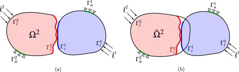
Figure 2: Continuum setting of two deformable bodies $\displaystyle\Omega^{1}$ and $\displaystyle\Omega^{2}$ coming into contact.

The gap function defines the signed distance between the two surfaces and is the fundamental measure that determines the status of contact. Here, we define the gap vector as a vector from a point $\displaystyle\underline{\bm{x}}^{1}$ on the surface $\displaystyle\Gamma_{c}^{1}$ to its closest fprojection $\displaystyle\hat{\underline{\bm{x}}}^{2}(\underline{\bm{x}}^{1})$ along the normal $\displaystyle\underline{\bm{n}}(\underline{\bm{x}}^{1})$ onto the surface $\displaystyle\Gamma_{c}^{2}$ (the choice of these surfaces is arbitrary):

$$\underline{\bm{g}}(\underline{\bm{x}}^{1},\Gamma_{c}^{2})=\hat{\underline{\bm{x}}}^{2}(\underline{\bm{x}}^{1})-\underline{\bm{x}}^{1}.$$ (6)

The normal gap function is thus obtained as a dot product of the gap vector $\displaystyle\underline{\bm{g}}$ (6) and the outward unit normal $\displaystyle\underline{\bm{n}}(\underline{\bm{x}}^{1})$

$$g_{n}(\underline{\bm{x}}^{1},\Gamma_{c}^{2})=\underline{\bm{g}}\cdot\underline{\bm{n}}(\underline{\bm{x}}^{1}).$$ (7)

The MorteX method is, at this stage, elaborated for two-dimensional problems only, which allows some simplifications in case of frictional contact, which is also presented in 2D. The tangential relative sliding velocity is given as in [47]:

$$\dot{g}_{\tau}(\underline{\bm{x}}^{1})=\underline{\bm{\tau}}(\underline{\bm{x}}^{1})\cdot\left(\dot{\underline{\bm{x}}}^{1}-\dot{\hat{\underline{\bm{x}}}}^{2}(\underline{\bm{x}}^{1})\right)$$ (8)

where $\displaystyle\underline{\bm{\tau}}(\underline{\bm{x}}^{1})$ is the unit tangential vector to $\displaystyle\Gamma_{c}^{1}$ at point $\displaystyle\underline{\bm{x}}^{1}$. In order to preserve the consistency of units, hereinafter the incremental slip will be used instead of the slip velocity $\displaystyle\mathring{g}_{\tau}=\dot{g}_{\tau}\Delta t$, where $\displaystyle 0<\Delta t<\infty$ is an arbitrary time increment. This replacement does not change the physical sense of all following equations. With these notations at hand, the contact traction can be decomposed into normal and tangential contributions:

$$\underline{\bm{t}}_{c}^{1}=p_{n}\underline{\bm{n}}+p_{\tau}\underline{\bm{\tau}}.$$ (9)

Along the contact interface, the classical Hertz-Signorini-Moreau conditions [35] also known as KKT conditions in the theory of optimization [30, 45] have to be satisfied. These conditions are formulated using the normal gap $\displaystyle g_{n}$ and the contact pressure $\displaystyle p_{n}$ as:

$$g_{n}\geq 0,\quad p_{n}\leq 0,\quad p_{n}g_{n}=0.$$ (10)

The tangential friction is described using the Coulomb friction law. The frictional constraints are formulated using the tangential slip increment $\displaystyle\mathring{g}_{\tau}$, the tangential traction $\displaystyle p_{\tau}$ and the contact pressure $\displaystyle p_{n}$. The incremental slip vanishes $\displaystyle|\mathring{g}_{\tau}|=0$ when the tangential traction is below the frictional threshold $\displaystyle|p_{\tau}|\leq\mu|p_{n}|$, non-zero incremental slip $\displaystyle|\mathring{g}_{\tau}|\neq 0$ is possible when $\displaystyle|p_{\tau}|=\mu|p_{n}|$. These conditions can be also formulated as KKT conditions:

$$|\mathring{g}_{\tau}|\geq 0,\quad|p_{\tau}|-\mu|p_{n}|\leq 0,\quad\left(\mu|p_{n}|-|p_{\tau}|\right)|\mathring{g}_{\tau}|=0$$ (11)

where $\displaystyle\mu$ is the Coulomb’s coefficient of friction.

3 Weak form

The Eqs. (1)-(3) denote the strong form of the standard solid mechanics BVP, and Eq. (4), along with the contact conditions (10)-(11) represents the contact part of the BVP. The weak form of the contact problem reduces to a variation inequality and the associated displacements should be selected in a constrained functional space, which has to include the non-penetration condition $\displaystyle g_{n}\geq 0$ [23, 35]. It is a constrained minimization problem. However, using the augmented Lagrangian method permits us to convert this problem into a fully unconstrained one, with displacements $\displaystyle\underline{\bm{u}}$ and virtual displacements $\displaystyle\delta\underline{\bm{u}}$ (test functions) selected in unconstrained functional spaces: $\displaystyle\mathcal{U}^{i}$ and the test function space $\displaystyle\mathcal{V}^{i}$ definitions:

$$\displaystyle\mathcal{U}^{i} \displaystyle=\{u^{i}\in H^{1}(\Omega^{i})\,|\,u^{i}=\hat{u}^{i}\,\mbox{on}\,\Gamma_{u}^{i}\},$$ (12)

$$\displaystyle\mathcal{V}^{i} \displaystyle=\{\delta u^{i}\in H^{1}(\Omega^{i})\,|\,\delta u^{i}=0\,\mbox{on}\,\Gamma_{u}^{i}\}$$ (13)

where $\displaystyle H^{1}(\Omega^{i})$ denotes the first order Sobolev space. The virtual work $\displaystyle\delta W_{s}$ corresponding to the structural part is given by:

$$\displaystyle\delta W_{s}=\sum_{i=1}^{2}\bigg{[}\underbrace{\int\limits_{\Omega^{i}}\underline{\underline{\bm{\sigma}}}^{i}:\delta\underline{\underline{\bm{\varepsilon}}}^{i}\,d\Omega^{i}}_{\delta W_{int}^{i}}-\underbrace{\int\limits_{\Omega^{i}}\underline{\bm{f}}_{v}^{i}\cdot\delta\underline{\bm{u}}^{i}\,d\Omega^{i}-\int\limits_{\Gamma_{t}^{i}}\hat{\underline{\bm{t}}}^{i}\cdot\delta\underline{\bm{u}}^{i}\,d\Gamma_{t}^{i}}_{\delta W_{ext}^{i}}\bigg{]},$$ (14)

where $\displaystyle\delta W_{\text{int}},\delta W_{\text{ext}}$ are the change in internal energy and the virtual work of forces, respectively.

Regarding the contribution of the virtual work associated with the contact problem, we adapt the monolithic augmented Lagrangian method (ALM) framework of Alart and Curnier [2] to the mortar framework. The ALM is a mixed dual formulation that introduces Lagrange multipliers as dual variables along with the primal displacement variables. The fields of Lagrange multipliers $\displaystyle\lambda_{n}$ and $\displaystyle\lambda_{\tau}$ are respectively equivalent to the contact pressure $\displaystyle p_{n}$ and the tangential friction shear $\displaystyle p_{\tau}$ introduced in Eq. (9). They and their virtual variations are selected from the appropriate functional space $\displaystyle\lambda_{n,\tau},\delta\lambda_{n,\tau}\in H^{-1/2}$, namely fractional Sobolev space of order $\displaystyle-1/2$. The augmented Lagrangian functionals $\displaystyle l_{n}$ and $\displaystyle l_{\tau}$ for the normal and frictional contact respectively are given by the following expressions [41, 42]:

$$l_{n}(g_{n},\lambda_{n})=\begin{cases}\lambda_{n}g_{n}+\frac{\varepsilon_{n}}{2}g_{n}^{2},\quad&\,\hat{\!\lambda}_{n}\leq 0,\\ -\frac{1}{2\varepsilon_{n}}\lambda_{n}^{2},\quad&\,\hat{\!\lambda}_{n}>0\end{cases}$$ (15)

$$l_{\tau}(\mathring{g}_{\tau},\lambda_{\tau},\,\hat{p}_{n})=\begin{cases}\begin{Bmatrix}&\lambda_{\tau}\mathring{g}_{\tau}+\frac{\varepsilon_{\tau}}{2}\mathring{g}_{\tau}^{2},&\quad|\,\hat{\!\lambda}_{\tau}|\leq-\mu\,\hat{p}_{n}\\ &-\frac{1}{2\varepsilon_{\tau}}\left(\lambda_{\tau}^{2}+2\mu\hat{p}_{n}|\,\hat{\!\lambda}_{\tau}|+\mu^{2}\hat{p}_{n}^{2}\right),&\quad|\,\hat{\!\lambda}_{\tau}|>-\mu\,\hat{p}_{n}\end{Bmatrix},&\,\hat{\!\lambda}_{n}\leq 0\\ -\frac{1}{2\varepsilon_{\tau}}\lambda_{\tau}^{2},&\,\hat{\!\lambda}_{n}>0\end{cases}$$ (16)

where $\displaystyle\,\hat{\!\lambda}_{n},\hat{\!\lambda}_{\tau},\hat{p}_{n}$ are the augmented normal and tangential Lagrange multipliers, and the augmented pressure, respectively:

$$\,\hat{\!\lambda}_{n}=\lambda_{n}+\varepsilon_{n}g_{n},\quad\,\hat{\!\lambda}_{\tau}=\lambda_{\tau}+\varepsilon_{\tau}\mathring{g}_{\tau},\quad\hat{p}_{n}=p_{n}+\varepsilon_{n}g_{n},$$ (17)

where $\displaystyle\varepsilon_{n}$ and $\displaystyle\varepsilon_{\tau}$ are the normal and tangential augmentation parameters, respectively. The augmented pressure determining the frictional threshold is replaced by the corresponding augmented Lagrange multiplier $\displaystyle\hat{\!\lambda}_{n}$, however $\displaystyle\hat{p}_{n}$ is not subjected to variation, therefore a different notation is used to highlight this subtle difference. Integrating the functionals (15) and (16) over the contact surface $\displaystyle\Gamma_{c}^{1}$ integrates the contact constraints in the Lagrangian:

$$\mathcal{L}=W_{s}+W_{c}=W_{s}+\int\limits_{\Gamma_{c}^{1}}l_{n}(g_{n},\lambda_{n})+l_{\tau}(\mathring{g}_{\tau},\lambda_{\tau},\hat{p}_{n})\,d\Gamma,$$ (18)

where $\displaystyle W_{s}$ is the potential energy of the system.

The problem of contrained optimization transforms into the min-max or saddle point problem for the Lagrangian, whose solution is equivalent to the solution of the variational inequality optimization problem on a non-convex domain and its boundary [30, 45, 41]. The min-max problem is solved by searching the stationary point minimizing the Lagrangian with respect to primal (displacement) field and maximizing it with respect to the dual field (Lagrange multipliers). The variation of the structural part, which contains only primal variables is given in (14), whereas the variation of the contact contribution is given by:

$$\displaystyle\delta W_{c} \displaystyle=\int\limits_{\Gamma_{c}^{1}}\delta l_{n}(g_{n},\lambda_{n})+\delta l_{\tau}(\mathring{g}_{\tau},\lambda_{\tau},\hat{p}_{n})\,d\Gamma_{c}^{1}=$$ (19)

$$\displaystyle=\int\limits_{\Gamma_{c}^{1}}\frac{\partial l_{n}}{\partial g_{n}}\delta g_{n}+\frac{\partial l_{\tau}}{\partial\mathring{g}_{\tau}}\delta\mathring{g}_{\tau}\,d\Gamma_{c}^{1}\,+$$ frictional contact virtual work (20)

$$\displaystyle\quad+\int\limits_{\Gamma_{c}^{1}}\frac{\partial l_{n}}{\partial\lambda_{n}}\delta\lambda_{n}\,d\Gamma_{c}^{1}\,+$$ weak normal contact contribution (21)

$$\displaystyle\quad+\int\limits_{\Gamma_{c}^{1}}\frac{\partial l_{\tau}}{\partial\lambda_{\tau}}\delta\lambda_{\tau}\,d\Gamma_{c}^{1} \displaystyle\quad\mbox{weak tangential contact contribution}.$$ (22)

The contact virtual work (19) is expressed as a summation of the contact contribution to the virtual work resulting from the variations of the positions (20), the weak contribution of normal contact constraints (21) from the variation of the normal Lagrange multiplier and the weak contribution of tangential contact constraints (22) from the variation of the tangential Lagrange multiplier. Note that the variations and derivatives of piece-wise smooth potentials $\displaystyle l_{n}$ and $\displaystyle l_{\tau}$ can be seen as sub-derivatives [41]. We recall that the variation of $\displaystyle\hat{p}_{n}$ is not required. Based on the three possible contact statuses (i.e. stick, slip or no contact), the contact surface is divided into three distinct sub-surfaces:

$$\Gamma_{c}^{1}=\Gamma_{{\mbox{\tiny stick}}}\,\cup\,\Gamma_{{\mbox{\tiny slip}}}\,\cup\,\Gamma_{{\mbox{\tiny nc}}}.$$

The frictional contact contribution to the virtual work can be split as follows:

$$\delta W_{c}=\begin{cases}\displaystyle\;\int\limits_{\Gamma_{{\mbox{\tiny stick}}}}\,\hat{\!\lambda}_{n}\delta g_{n}+g_{n}\delta\lambda_{n}+\,\hat{\!\lambda}_{\tau}\delta\mathring{g}_{\tau}+\mathring{g}_{\tau}\delta\lambda_{\tau}\,d\Gamma,&{\hat{\!\lambda}_{n}\leq 0,\;}|\,\hat{\!\lambda}_{\tau}|\leq-\mu\,\hat{p}_{n},\mbox{ stick,}\\ \displaystyle\;\int\limits_{\Gamma_{{\mbox{\tiny slip}}}}\,\hat{\!\lambda}_{n}\delta g_{n}+g_{n}\delta\lambda_{n}-\mu\,\hat{p}_{n}\mathrm{sign}(\,\hat{\!\lambda}_{\tau})\delta\mathring{g}_{\tau}-\frac{1}{\varepsilon_{\tau}}\bigg{(}\lambda_{\tau}+\mu\,\hat{p}_{n}\mathrm{sign}(\,\hat{\!\lambda}_{\tau})\bigg{)}\;\delta\lambda_{\tau}\,d\Gamma,&{\hat{\!\lambda}_{n}\leq 0,\;}|\,\hat{\!\lambda}_{\tau}|>-\mu\,\hat{p}_{n},\mbox{slip,}\\ \displaystyle\;\int\limits_{\Gamma_{{\mbox{\tiny nc}}}}-\frac{1}{\varepsilon_{n}}\lambda_{n}\delta\lambda_{n}-\frac{1}{\varepsilon_{\tau}}\lambda_{\tau}\delta\lambda_{\tau}{\,d\Gamma},&\,\hat{\!\lambda}_{n}>0.\end{cases}$$ (23)

4 Mortar interface discretization

Within the mortar discretized framework, the contacting surfaces are typically classified into mortar and non-mortar sides. In the following, the superscript “$\displaystyle 1$” refers to the mortar side of the interface and “$\displaystyle 2$” to the non-mortar side. The choice of mortar and non-mortar is rather arbitrary: however, in general the choice of the finer meshed surface as mortar side is known to result in higher accuracy. All the contact related integral evaluations will be carried out on the mortar side of the interface. In the considered two dimensional case, the edges of potentially contacting surfaces are parametrized by $\displaystyle\xi^{i}\,\in[-1;1]$ . In the current configuration the interpolations of mortar and non-mortar surface edges are given by:

$$\underline{\bm{x}}^{1}(\xi^{1},t)=N^{1}_{m}(\xi^{1})\underline{\bm{x}}_{m}^{1},\quad{\underline{\bm{x}}^{2}(\xi^{2},t)=N^{2}_{i}(\xi^{2})\underline{\bm{x}}_{i}^{2},\quad m\in[1,\mathrm{M}],\;i\in[1,\mathrm{N}]}.$$ (24)

$\displaystyle N^{1}_{m}(\xi^{1})$ and $\displaystyle N^{2}_{i}(\xi^{2})$ are the interpolation functions of mortar and non-mortar sides, respectively; whereas $\displaystyle\mathrm{M}$ and $\displaystyle\mathrm{N}$ is the number of nodes per segment at mortar and non-mortar sides, respectively. Note that we use isoparametric linear elements, which implies that the normal remains constant along the edge. Moreover, that in the current framework, for the sake of simplicity, we omitted averaging of normals at nodes and their interpolation, which was elaborated in [58, 43]. Hereinafter, Einstein summation over repetitive index is used. We assign scalar Lagrange multipliers $\displaystyle\lambda_{n}$ and $\displaystyle\lambda_{\tau}$ for the normal and tangential directions to the nodes of the mortar side. The Lagrange multiplier vector $\displaystyle\underline{\bm{\lambda}}=\lambda_{n}\underline{\bm{n}}+\lambda_{\tau}\underline{\bm{\tau}}$ is interpolated functions $\displaystyle\Phi_{l}$:

$${\underline{\bm{\lambda}}(\xi^{1},t)=\Phi_{l}(\xi^{1})\underline{\bm{\lambda}}^{l}(t),\quad l\in[1,\mathrm{L}]}$$ (25)

where $\displaystyle\mathrm{L}$ is the number of nodes used for interpolation over every edge, where L can be less than or equal to M.

Every mortar contact element is created between parts of mortar and non-mortar segments which are projected one on the other (see Fig. 3). The segment-to-segment projection is described in detail in [57, 58, 44] and will not be reproduced here. Each contact element consists of $\displaystyle\mathrm{M+N}$ nodes, each with $\displaystyle 2$ primal DoFs in 2D, and of $\displaystyle\mathrm{L}$ or $\displaystyle 2\mathrm{L}$ dual DoFs associated with Lagrange multipliers in case of frictionless or frictional contact, respectively.

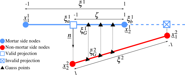
Figure 3: Nodes of the non-mortar edge are projected onto mortar edge, establishing a mapping and determining the integration domain parametrized by $\displaystyle\zeta$.

4.1 Discrete integral kinematic quantities

As a first step towards the elaboration of the contact part of the residual vector, the discretisations (24) and (25) are inserted in the continuous weak form (23). First, we focus on the derivation of a single term of this integral, which enables us to introduce coincise notations and simplifications to be used for the other terms. It is obtained for every active contact element by integrating over a part or an entire mortar edge $\displaystyle S^{\mathrm{el}}$:

$$\int\limits_{S^{\mathrm{el}}}g_{n}\delta\lambda_{n}\,d\Gamma=\int\limits_{S^{\mathrm{el}}}\left(N^{1}_{m}(\xi^{1})\underline{\bm{x}}^{1}_{m}-N^{2}_{i}(\xi^{2})\underline{\bm{x}}^{2}_{i}\right)\cdot\underline{\bm{n}}\,\Phi_{l}(\xi^{1})\delta\lambda^{l}_{n}\,d\Gamma$$ (26)

where $\displaystyle\underline{\bm{n}}$ is the unit outward normal of the mortar edge. Note that this equality holds if the parametrization $\displaystyle\xi^{2}$ ensures collinearity between the vector in brackets and the normal vector. Therefore, $\displaystyle\xi^{2}$ depends on positions of all the nodes both mortar and non-mortar forming the contact element. This is not explicitly reflected in the equation but should be kept in mind. The hat-notations, which denoted projections in (6,8), are therefore omitted hereinafter.

It appears useful [47] to introduce an integral gap vector $\displaystyle\bar{\!\underline{\bm{g}}}^{l}$, which is defined using the above Eq. (26) as:

$${\bar{\!\underline{\bm{g}}}^{l}(t)}=\left[{D}_{lm}\underline{\bm{x}}_{m}^{1}-{M}_{li}\underline{\bm{x}}_{i}^{2}\right]$$ (27)

where $\displaystyle D_{lm}$ and $\displaystyle M_{li}$ are the so-called mortar integrals [44], which are defined as
$$D_{lm}=\int\limits_{S^{\mathrm{el}}}\Phi_{l}(\xi^{1})N^{1}_{m}(\xi^{1})\,d\Gamma,\quad$$ (28) $$M_{li}=\int\limits_{S^{\mathrm{el}}}\Phi_{l}(\xi^{1})N^{2}_{i}(\xi^{2})\,d\Gamma.$$ (29) The evaluation of the these integrals forms the core of the mortar discretization scheme. The evaluation of these integrals is detailed in Section 4.2. Using the introduced notations, the term (26) takes a simple form:

$$\int\limits_{S^{\mathrm{el}}}g_{n}\delta\lambda_{n}\,d\Gamma=\bar{\!g}_{n}^{l}\delta\lambda^{l}_{n}$$ (30)

where

$$\bar{g}_{n}^{l}=\bar{\underline{\bm{g}}}^{l}\cdot\underline{\bm{n}}=\left[D_{lm}\underline{\bm{x}}^{1}_{m}-M_{li}\underline{\bm{x}}^{2}_{i}\right]\cdot\underline{\bm{n}}$$ (31)

is the integral normal gap. The variation of the integral normal gap is given by:

$$\delta\bar{\!g}_{n}^{l}=\left[{D}_{lm}\delta\underline{\bm{x}}_{m}^{1}-{M}_{li}\delta\underline{\bm{x}}_{i}^{2}\right]\cdot\underline{\bm{n}}.$$ (32)

By analogy, the contribution of the tangential contact term can be introduced as:

$$\int\limits_{S^{\mathrm{el}}}\mathring{g}_{\tau}\delta\lambda_{\tau}\,d\Gamma=\mathring{\bar{\!g}}_{\tau}^{l}\delta\lambda^{l}_{\tau},$$ (33)

where $\displaystyle\mathring{\bar{g}}_{\tau}^{l}$ is the integral slip increment given by [47]:

$$\begin{split}\mathring{\bar{\!g}}_{\tau}^{l}(t_{j})&=-\underline{\bm{\tau}}_{l}(t_{j})\cdot\bigg{(}[D_{lm}(t_{j})-D_{lm}(t_{j-1})]\underline{\bm{x}}_{m}^{1}(t_{j-1})-[M_{li}(t_{j})-M_{li}(t_{j-1})]\underline{\bm{x}}_{i}^{2}(t_{j-1})\bigg{)}=\\ &=-\underline{\bm{\tau}}_{l}(t_{j})\cdot\left(D_{lm}(t_{j})\underline{\bm{x}}_{m}^{1}(t_{j-1})-M_{li}(t_{j})\underline{\bm{x}}_{i}^{2}(t_{j-1})-\underline{\bm{g}}^{l}(t_{j-1})\right)\end{split}$$ (34)

where the current time step $\displaystyle t_{j}$ and the previous time step $\displaystyle t_{j-1}$ come in an interplay. The variation of the incremental slip, again following [47] is given by:

$$\delta\mathring{\bar{g}}_{\tau}^{l}(t_{j})=\underline{\bm{\tau}}_{l}(t_{j})\cdot\bigg{(}D_{lm}(t_{j})\delta\underline{\bm{x}}_{m}^{1}-M_{li}(t_{j})\delta\underline{\bm{x}}_{i}^{2}\bigg{)}.$$ (35)

Eqs. (32) and (35) are both used for evaluation of Eq. (23).

4.2 Evaluation of mortar integrals

The evaluation of the mortar side integrals $\displaystyle D_{lm}$ is straightforward, as it only involves the product of shape functions from the mortar side (28). This is in contrast with the evaluation of the mortar integral $\displaystyle M_{li}$ which combines shape functions from both the mortar and non-mortar sides. Its evaluation requires a mapping between them (Fig. 3). For this purpose, non-mortar quantities are projected onto the mortar side of the interface using the mortar segment normal vector. The non-mortar nodes $\displaystyle\underline{\bm{x}}_{i}^{2}\,(i\,\in[1,N])$ are projected onto the mortar side segment along the mortar segment normal $\displaystyle\underline{\bm{n}}$. The local coordinates $\displaystyle\xi^{1}_{i}$ of the projections are found by solving

$$\left(N^{1}_{m}(\xi_{i}^{1})\underline{\bm{x}}^{1}_{m}-\underline{\bm{x}}_{i}^{2}\right)\times\underline{\bm{n}}=0.$$ (36)

The extremities of the integration domain $\displaystyle S^{\mathrm{el}}$ are defined either by mortar or non-mortar edge nodes, details of this procedure are provides in [58] and not repeated here. The segment of the mortar edge over which the evaluation of mortar integrals is carried out is parametrized by $\displaystyle\zeta\in[-1;1]$. The projection coordinates $\displaystyle\xi_{a/b}^{1}$, which determine the limits of the integration domain, are mapped on the segment parameterization:

$$\xi^{1}(\zeta)=\frac{1}{2}(1-\zeta)\xi_{a}^{1}\,+\,\frac{1}{2}(1+\zeta)\xi_{b}^{1}.$$ (37)

Fig. 3 illustrates how the integration domain is determined between two edges. To evaluate the integrals using Gauss quadratures, the mortar-side Gauss points $\displaystyle\xi^{1}_{G}$ are projected along mortar segment normal $\displaystyle\underline{\bm{n}}$ onto the non-mortar side and the corresponding local coordinates $\displaystyle\zeta_{G}$ are determined by:

$$\left[N^{2}_{i}(\xi^{2}_{G})\underline{\bm{x}}^{2}_{i}-N^{1}_{m}(\xi^{1}_{G})\underline{\bm{x}}^{1}_{m}\right]\times\underline{\bm{n}}=0.$$ (38)

The mortar matrices, evaluated with Gauss quadratures, take the following form:

$$D_{lm}=\int\limits_{S^{\mathrm{el}}}\Phi_{l}(\xi^{1})N^{1}_{m}(\xi^{1})\,d\Gamma=w_{G}\Phi_{l}(\xi^{1}_{G})N^{1}_{m}(\xi^{1}_{G})J_{\mbox{\tiny seg}}(\xi_{G}^{1}),$$ (39)

$$M_{li}=\int\limits_{S^{\mathrm{el}}}\Phi_{l}(\xi^{1})N^{2}_{i}(\xi^{2})\,d\Gamma=w_{G}\Phi_{l}(\xi^{1}_{G})N^{2}_{i}(\xi^{2}_{G})J_{\mbox{\tiny seg}}(\xi_{G}^{1}),$$ (40)

where, as previously, $\displaystyle l\in[1,L]$, $\displaystyle m\in[1,M]$, $\displaystyle i\in[1,N]$ and $\displaystyle G\in[1,N_{G}]$, where $\displaystyle N_{G}$ is number of Gauss integration points, $\displaystyle J_{\mbox{\tiny seg}}$ is the normalized Jacobian

$$J_{\mbox{\tiny seg}}(\xi_{G}^{1})=\bigg{|}\frac{\partial{N^{1}_{i}}}{\partial\xi^{1}}\frac{\partial\xi^{1}}{\partial\zeta}\underline{\bm{X}}_{i}\bigg{|}.$$ (41)

The factor $\displaystyle\partial\xi^{1}/\partial\zeta$ reflects the fact that the integral is evaluated only over a part of the mortar edge.

4.3 Residual vector

Within the augmented Lagrangian formulation, every created contact element contributes to the virtual work of the system irrespectively of its contact status (active or inactive). This translates into a smoother energy potential in comparison to the standard method of Lagrange multipliers. For each contact element, the discretized form of the virtual work can be obtained for the three possible contact statuses, namely stick, slip and no contact as follows:

$$\displaystyle\delta W_{\mbox{\tiny stick}}^{e}= \displaystyle\begin{bmatrix}\delta\underline{\bm{x}}_{m}^{1}\\[3.0pt] \delta\underline{\bm{x}}_{i}^{2}\\[3.0pt] \delta\lambda_{n}^{l}\\[3.0pt] \delta\lambda_{\tau}^{l}\\ \end{bmatrix}^{\intercal}\begin{bmatrix}D_{lm}\bigg{(}\hat{\!\lambda}_{n}^{l}\underline{\bm{n}}+\hat{\!\lambda}_{\tau}^{l}\underline{\bm{\tau}}\bigg{)}\\ -M_{li}\bigg{(}\hat{\!\lambda}_{n}^{l}\underline{\bm{n}}+\hat{\!\lambda}_{\tau}^{l}\underline{\bm{\tau}}\bigg{)}\\ \bar{g}_{n}^{l}\\[3.0pt] \mathring{\bar{g}}_{\tau}^{l}\\ \end{bmatrix}, \displaystyle\quad\hat{\!\lambda}_{n}^{l}\leq 0,\,|\,\hat{\!\lambda}_{\tau}^{l}|\leq-\mu\,\hat{\!\lambda}_{n}^{l}\,(\mbox{stick})$$ (42)

$$\displaystyle\delta W_{\mbox{\tiny slip}}^{e}= \displaystyle\begin{bmatrix}\delta\underline{\bm{x}}_{m}^{1}\\[3.0pt] \delta\underline{\bm{x}}_{i}^{2}\\[3.0pt] \delta\lambda_{n}^{l}\\[3.0pt] \delta\lambda_{\tau}^{l}\\ \end{bmatrix}^{\intercal}\begin{bmatrix}D_{lm}\bigg{(}\hat{\!\lambda}_{n}^{l}\underline{\bm{n}}-\mu\,\hat{\!\lambda}_{n}^{l}\mathrm{sign}(\,\hat{\!\lambda}_{\tau})\underline{\bm{\tau}}_{l}\bigg{)}\\ -M_{li}\bigg{(}\hat{\!\lambda}_{n}^{l}\underline{\bm{n}}-\mu\,\hat{\!\lambda}_{n}^{l}\mathrm{sign}(\,\hat{\!\lambda}_{\tau})\underline{\bm{\tau}}_{l}\bigg{)}\\ \bar{g}_{n}^{l}\\ -\frac{1}{\varepsilon_{\tau}}\left(\lambda_{\tau}^{l}+\mu\,\hat{\!\lambda}_{n}^{l}\mathrm{sign}(\,\hat{\!\lambda}_{\tau}^{l})\right)\end{bmatrix}, \displaystyle\quad\hat{\!\lambda}_{n}^{l}\leq 0,\,|\,\hat{\!\lambda}_{\tau}^{l}|>-\mu\,\hat{\!\lambda}_{n}^{l}\,(\mbox{slip})$$ (43)

$$\displaystyle\delta W_{\mbox{\tiny nc}}^{e}= \displaystyle\begin{bmatrix}\delta\underline{\bm{x}}_{m}^{1}\\[3.0pt] \delta\underline{\bm{x}}_{i}^{2}\\[3.0pt] \delta\lambda_{n}^{l}\\[3.0pt] \delta\lambda_{\tau}^{l}\\ \end{bmatrix}^{\intercal}\begin{bmatrix}0\\ 0\\ -\frac{1}{\varepsilon_{n}}\lambda_{n}^{l}\\[10.0pt] -\frac{1}{\varepsilon_{\tau}}\lambda_{\tau}^{l}\\ \end{bmatrix}, \displaystyle\quad\hat{\!\lambda}_{n}^{l}>0\,(\mbox{no contact}).$$ (44)

It is important to remark that the contact status is now based on the integral quantities (31, 34).

$$\hat{\lambda}_{n}^{l}=\lambda_{n}^{l}+\varepsilon_{n}\bar{g}_{n}^{l},\quad\hat{\lambda}_{\tau}^{l}=\lambda_{\tau}^{l}+\varepsilon_{\tau}\mathring{\bar{g}}_{\tau}^{l}.$$

5 Extended finite element methods

In this section, we present some elements of the extended finite element method (X-FEM) [18, 9]. In complement to the mortar method, X-FEM is a key ingredient required to construct a unified MorteX framework to treat contact problems along along surfaces embedded in the bulk mesh. By analogy with the MorteX method for tying [1], the mesh hosting the embedded surface will be referred to as the host mesh. Such an embedded (or virtual) surface splits the domain of the host solid into two parts. One part is discarded (i.e. considered as empty space) and the remaining effective part represents the solid, see Fig. 4. The virtual line $\displaystyle\tilde{\Gamma}_{c}^{2}$ runs through elements, which will be called blending elements. As such, these elements are also made of discarded and effective parts. The finite elements are then essentially partitioned into three distinct categories, namely the discarded, blending and standard elements. Here, X-FEM will be used to account for the fact that only the effective volume $\displaystyle\tilde{\Omega}^{2}$ contributes to the internal virtual work.

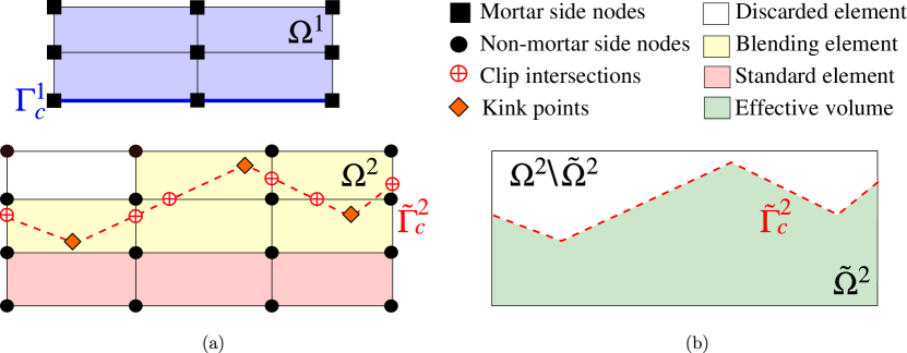
Figure 4: (a) Discrete contact interface pair: $\displaystyle\Gamma_{c}^{1}$ and $\displaystyle\Gamma_{c}^{2}$ denote real mortar surface and embedded non-mortar surface, respectively; (b) effective volume of the host domain $\displaystyle\tilde{\Omega}^{2}$.

The virtual surface $\displaystyle\tilde{\Gamma}^{2}_{c}$ of the host domain is treated as an internal discontinuity, the outer part of the volume $\displaystyle\Omega^{2}\setminus\tilde{\Omega}^{2}$ is disregarded using the X-FEM framework. The X-FEM relies on enhancement of the FEM shape functions used to interpolate the displacement fields. The enrichment functions describing the field behavior are incorporated locally into the finite element approximation. This feature allows the resulting displacement to capture discontinuities. The subdivision of the host mesh is defined by indicator function $\displaystyle\phi({\underline{\bm{X}}}):\mathbb{R}^{\mathrm{dim}}\to\{0,1\}$ (where $\displaystyle{\underline{\bm{X}}}$ is the spatial position vector in the reference configuration in domain $\displaystyle\Omega^{2}$) [51]. The indicator function is non-zero only in the efficient part of the host domain $\displaystyle\tilde{\Omega}^{2}$:

$$\phi(\underline{\bm{X}})=\begin{cases}1,&\mbox{ if }\underline{\bm{X}}\in\tilde{\Omega}^{2};\\ 0,&\mbox{ elsewhere.}\end{cases}$$

The discontinuity surface $\displaystyle\tilde{\Gamma}^{2}_{c}$ can be seen as a level-set defined as follows:

$$\tilde{\Gamma}^{2}_{g}=\left\{\underline{\bm{X}}\in\Omega^{2}:\;\nabla\phi(\underline{\bm{X}})\neq 0\right\}.$$

In the considered framework, for the sake of simplicity, we will assume that the embedded surface is represented by a piece-wise linear line with possible kink points occurring inside host elements.

In practice, the enrichment of shape functions in case of void/inclusion problem can be simply replaced by a selective integration scheme [53]. For the standard elements, there is no change in volume of integration and the discarded elements are simply excluded from the volume integration procedure. In order to obtain the effective volume of integration for each blending element, we perform the clipping of the blending elements by the embedded surface $\displaystyle\tilde{\Gamma}^{2}_{c}$ [Fig. 5] . The clipped element is virtually triangulated to perform the integration of the internal virtual work using a Gauss quadrature rule. In this framework, we use three newly initialized Gauss points per triangle which ensures a rather accurate integration in view of linear or bi-linear shape functions for triangular and quadrilateral elements, respectively. The clipping of a single element by an arbitrary embedded surface results in one or several various polygons either convex or non-convex or even disjoint, which represent the effective volumes of integration. The tilde ($\displaystyle\tilde{\bullet}$) notations are adopted for the quantities related to the effective part of the host mesh ($\displaystyle\tilde{\Omega}^{2}$).

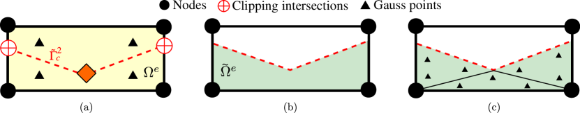
Figure 5: Selective integration scheme for blending elements: (a) blending element with standard Gauss points; (b) elemental volume segregation based on polygon clipping (shaded part represents the effective volume); (c) triangulation of the effective volume, and reinitialization of Gauss points, which is used to evaluate associated integrals using a Gauss quadrature rule.

6 MorteX framework

Here, the MorteX framework, which is presented in a separate paper [1] in the context of mesh tying problems, is extended to treat frictional contact problems. Similar to the tying problem, it consists of two distinct procedures. The first procedure invokes the X-FEM method to account for the fact that only a portion of the body $\displaystyle\Omega^{2}$ is contributing to the internal virtual work; it is called the effective volume, see $\displaystyle\tilde{\Omega}^{2}$ on Fig. 4. The second procedure deals with the enforcement of the contact constraints between a “real” surface $\displaystyle\Gamma_{c}^{1}$ (explicitly represented by edges) and an embedded virtual surface $\displaystyle\Gamma^{2}_{c}$, which is geometrically non-conformal with the finite element discretization and passing through the elements. The contact treatment is adjusted through few modifications of the classical mortar contact schemes introduced in Section 4.

6.1 MorteX interface discretization

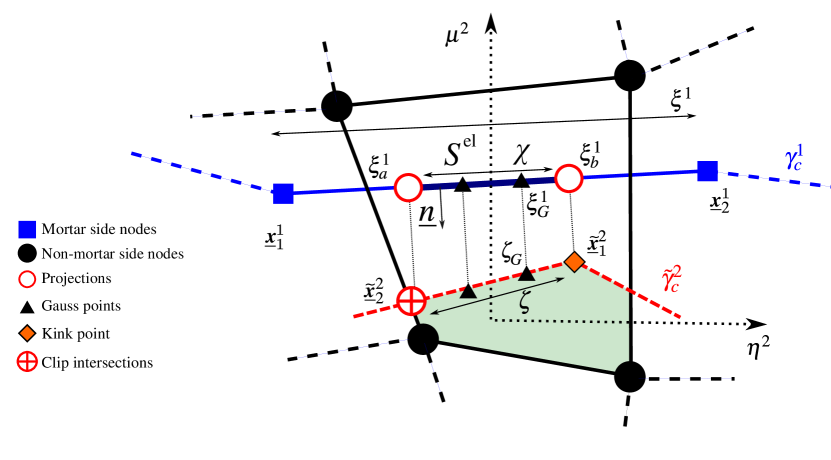
Figure 6: Example of mortar domain: the contact element is formed between a mortar side segment connecting $\displaystyle\underline{\bm{x}}_{1}^{1}$ and $\displaystyle\underline{\bm{x}}_{2}^{1}$ and a blending element; the integration is carried out over a portion of mortar segment and a corresponding portion of embedded surface (dashed line) between a clip intersection $\displaystyle\tilde{\underline{\bm{x}}}_{2}^{1}$ and a kink point $\displaystyle\tilde{\underline{\bm{x}}}_{1}^{2}$.

Similar to the tying problem in the MorteX framework, the rationale behind the choice of mortar and non-mortar sides, holds for the contact problems as well [1]: the real surface is always selected as the mortar surface. The interpolations of the nodal positions in the current configuration and the Lagrange multipliers along the mortar side $\displaystyle\Gamma_{c}^{1}$ remain the same as for the classical schemes, and are given by:

$$\underline{\bm{x}}^{1}(\xi^{1})=N_{m}(\xi^{1})\underline{\bm{x}}_{m}^{1},\quad m\in[1,\mathrm{M}],$$ (45)

$$\lambda_{n,\tau}(\xi^{1})=\Phi_{l}(\xi^{1})\lambda^{l}_{n,\tau},\quad l\in[1,\mathrm{L}].$$ (46)

where as previously $\displaystyle\mathrm{M}$ and $\displaystyle\mathrm{L}$ is the number of nodes per mortar segment and those carrying Lagrange multipliers respectively. Vector $\displaystyle\underline{\bm{x}}_{m}^{1}$ represents the nodal positions of the mortar nodes forming the segment, and $\displaystyle\xi^{1}\in[-1;1]$ is the parametric coordinate of the mortar side. The parametrization on the non-mortar side requires more consideration. As shown in Fig. 6, the embedded surface $\displaystyle\tilde{\Gamma}_{c}^{2}$ is divided into straight segments, whose vertices can either be a clip intersection (i.e. the intersection between $\displaystyle\tilde{\Gamma}_{c}^{2}$ and the edge of a bulk element of the non-mortar side) or a kink point (a vertex of the discrete virtual surface $\displaystyle\tilde{\Gamma}_{c}^{2}$ that lies inside a blending element). Hereinafter, we will refer to these vertices as “points of interest”, without distinction between kink and clip intersection points; their notation will be equipped with a tilde $\displaystyle\tilde{\underline{\bm{x}}}_{j}^{2},j\in[1,2]$. The shape of the embedded surface in the current configuration parametrized by $\displaystyle\zeta\in[-1;1]$ between two points of interest, can be defined using two-dimensional shape functions inherited from the host element [see Fig. 6]:

$${\underline{\bm{x}}}^{2}(\zeta)=N_{i}\left(\mu^{2}(\zeta),\eta^{2}(\zeta)\right)\underline{\bm{x}}_{i}^{2}.$$ (47)

Irrespective of the fact that the embedded surface is assumed piece-wise linear in the reference configuration, it can become piece-wise non-linear in the current configuration, therefore the displacement along every linear segment cannot be parametrized by linear shape functions. Note that here, in the MorteX contact set-up, the kink points represent vertices of the discretized surface $\displaystyle\tilde{\Gamma}_{c}^{2}$, whereas they represented imprints of mortar side nodes in case of MorteX tying set-up [1].

6.1.1 MorteX contact element

A MorteX contact element is formed between a single mortar segment and a blending element, and it consists of $\displaystyle(\mathrm{M}+\mathrm{N})$ nodes, $\displaystyle\mathrm{M}$ from the mortar segment, and $\displaystyle\mathrm{N}$ from blending element. In addition the contact element stores $\displaystyle\mathrm{L}$ or $\displaystyle\mathrm{L}\times\mathrm{dim}$ Lagrange multipliers for the frictionless and frictional cases, respectively. As was shown in [1], to avoid mesh-locking (or over-constraining of the interface), which results in spurious oscillations, the number of Lagrange multipliers should be balanced by the number of blending elements, i.e. often it is reasonable to use one set per blending element, a detailed discussion can be found in Section 7.

6.1.2 Discrete integral kinematic quantities

The aforementioned selective integration scheme, used to accommodate for the presence of an embedded virtual surface, leads to changes in the discrete contact integral quantities: the integral gap vector (27), the integral normal gap (31) and the incremental slip (34). For a MorteX contact element, these nodal quantities are now evaluated along the interface formed by a pair of real and embedded segments (tilde-notations are used):

$$\displaystyle{\tilde{\bar{\!\underline{\bm{g}}}}^{l}} \displaystyle=\left[{D}_{lm}\underline{\bm{x}}_{m}^{1}-\tilde{{M}}_{li}{\underline{\bm{x}}}_{i}^{2}\right],$$ (48)

$$\displaystyle\tilde{\bar{g}}_{n}^{l} \displaystyle=\tilde{\bar{\underline{\bm{g}}}}^{l}\cdot\underline{\bm{n}},$$ (49)

$$\displaystyle\mathring{\tilde{\bar{g}}}^{l}_{\tau} \displaystyle=-\underline{\bm{\tau}}\cdot\left[\left(D_{lm}(t_{j})-D_{lm}(t_{j-1})\right){\underline{\bm{x}}}_{m}^{1}(t_{j-1})-\left(\tilde{M}_{li}(t_{j})-\tilde{M}_{li}(t_{j-1})\right){\underline{\bm{x}}}_{i}^{2}(t_{j-1})\right]$$ (50)

where $\displaystyle i\in[1,N]$, $\displaystyle l\in[1,L]$, $\displaystyle m\in[1,M]$, $\displaystyle{D}_{lm}$ and $\displaystyle\tilde{M}_{li}$ are the mortar integrals in the MorteX framework, which will be defined in (58). Note that within the MorteX framework, the definitions of purely mortar side quantities, like the mortar segment normal $\displaystyle\underline{\bm{n}}$ and mortar side integral $\displaystyle D_{lm}$ remain the same as in the classical mortar framework, whereas $\displaystyle\tilde{M}_{lm}$ now presents a convolution of volumetric and surface shape functions of primal and dual quantities, respectively.

6.1.3 Discrete contact virtual work

The MorteX residual vector is larger than the standard mortar one as it involves the displacement DoFs from the bulk of the non-mortar side of the interface. The residuals for stick, slip and non-contact statuses are:

$$\displaystyle\delta\tilde{W}_{\mbox{\tiny stick}}^{\mathrm{el}}= \displaystyle\begin{bmatrix}\delta\underline{\bm{x}}_{m}^{1}\\[5.0pt] \delta\underline{\bm{x}}_{i}^{2}\\[5.0pt] \delta\lambda_{n}^{l}\\[5.0pt] \delta\lambda_{\tau}^{l}\\ \end{bmatrix}^{\intercal}\begin{bmatrix}\left(\hat{\!\lambda}_{n}^{l}\underline{\bm{n}}+\hat{\!\lambda}_{\tau}^{l}\underline{\bm{\tau}}\right)D_{lm}\\[5.0pt] -\left(\hat{\!\lambda}_{n}^{l}\underline{\bm{n}}+\hat{\!\lambda}_{\tau}^{l}\underline{\bm{\tau}}\right)\tilde{M}_{li}\\[5.0pt] \tilde{\bar{g}}_{n}^{l}\\[5.0pt] \mathring{\tilde{\bar{g}}}_{\tau}^{l}\\ \end{bmatrix}, \displaystyle\quad\hat{\!\lambda}_{n}^{l}\leq 0,\,|\,\hat{\!\lambda}_{\tau}^{l}|\leq-\mu\,\hat{\!\lambda}_{n}^{l}\,(\mbox{stick})$$ (51)

$$\displaystyle\delta\tilde{W}_{\mbox{\tiny slip}}^{e}= \displaystyle\begin{bmatrix}\delta\underline{\bm{x}}_{m}^{1}\\[5.0pt] \delta\underline{\bm{x}}_{i}^{2}\\[5.0pt] \delta\lambda_{n}^{l}\\[5.0pt] \delta\lambda_{\tau}^{l}\\ \end{bmatrix}^{\intercal}\begin{bmatrix}\left(\hat{\!\lambda}_{n}^{l}\underline{\bm{n}}-\mu\,\hat{\!\lambda}_{n}^{l}\mathrm{sign}(\,\hat{\!\lambda}_{\tau})\underline{\bm{\tau}}\right)D_{lm}\\[5.0pt] -\left(\hat{\!\lambda}_{n}^{l}\underline{\bm{n}}-\mu\,\hat{\!\lambda}_{n}^{l}\mathrm{sign}(\,\hat{\!\lambda}_{\tau})\underline{\bm{\tau}}\right)\tilde{M}_{li}\\[5.0pt] \tilde{\bar{g}}_{n}^{l}\\[5.0pt] -\frac{1}{\varepsilon_{\tau}}\left(\lambda_{\tau}^{l}+\mu\,\hat{\!\lambda}_{n}^{l}\mathrm{sign}(\,\hat{\!\lambda}_{\tau}^{l})\right)\end{bmatrix}, \displaystyle\quad\hat{\!\lambda}_{n}^{l}\leq 0,\,|\,\hat{\!\lambda}_{\tau}^{l}|>-\mu\,\hat{\!\lambda}_{n}^{l}\,(\mbox{slip})$$ (52)

$$\displaystyle\delta\tilde{W}_{\mbox{\tiny nc}}^{e}= \displaystyle\begin{bmatrix}\delta\underline{\bm{x}}_{m}^{1}\\[5.0pt] \delta\underline{\bm{x}}_{i}^{2}\\[5.0pt] \delta\lambda_{n}^{l}\\[5.0pt] \delta\lambda_{\tau}^{l}\\ \end{bmatrix}^{\intercal}\begin{bmatrix}0\\ 0\\ -\frac{1}{\varepsilon_{n}}\lambda_{n}^{l}\\[5.0pt] -\frac{1}{\varepsilon_{\tau}}\lambda_{\tau}^{l}\\ \end{bmatrix}, \displaystyle\quad\hat{\!\lambda}_{n}^{l}>0\,(\mbox{no contact}).$$ (53)

In addition, the contact detection as well as the evaluation of the residual vector are based on the following modified weighted integral quantities (48), (49) and (50).

$$\hat{\lambda}_{n}^{l}=\lambda_{n}^{l}+\varepsilon_{n}\tilde{\bar{g}}_{n}^{l},\quad\hat{\lambda}_{\tau}^{l}=\lambda_{\tau}^{l}+\varepsilon_{\tau}\mathring{\tilde{\bar{g}}}_{\tau}^{l}.$$

6.1.4 MorteX integral evaluation

The numerical procedures of the classical mortar framework to evaluate the mortar integrals need to be adapted for the MorteX framework similar to what was done for the tying problem. However, the numerical procedure adapted for the tying problem in MorteX framework cannot be used directly for the contact problems, because the former does not require any projections between the tying surfaces $\displaystyle\tilde{\Gamma}_{g}^{2}$ and $\displaystyle\Gamma_{g}^{1}$ [1]. The lack of projections in the tying framework is due to the fact that the embedded surface is nothing but an imprint of the mortar surface of the patch domain in the reference configuration. However, for the non-linear contact problem, where the contact interface continuously changes in response to the deformations the bodies, the conformity of surface meshes cannot be ensured. It implies a need for a projection step similar to the classical mortar framework to determine the limits of integration mortar-domain $\displaystyle S^{\mathrm{el}}$ (see Fig. 6). The quantities projected are points of interest rather than non-mortar segment nodes, which is the case in the classical mortar. The mortar projection coordinates for the extremities of the integration ($\displaystyle\xi^{1}_{a},\xi^{2}_{b}$) are found by solving the following equation:

$${\left[N_{m}(\xi^{1})\underline{\bm{x}}^{1}_{m}-\tilde{\underline{\bm{x}}}^{2}_{i}\right]\times\underline{\bm{n}}=0},$$ (54)

where $\displaystyle\tilde{\underline{\bm{x}}}^{2}$ denote points of interest (kink or clip intersection). The resulting projections $\displaystyle\xi_{a/b}^{1}$ serve as limits of the mortar domain $\displaystyle S^{\mathrm{el}}$, which is parametrized by $\displaystyle\chi\,\in[-1,1]$ (see Fig. 6). To evaluate the integrals using Gauss quadrature, the mortar-side Gauss points $\displaystyle\xi^{1}_{G}$ are projected along the mortar-segment normal $\displaystyle\underline{\bm{n}}$ onto the non-mortar side. The corresponding local coordinates $\displaystyle\zeta_{G}$ are determined by solving for each Gauss point $\displaystyle\xi^{1}_{G}$:

$$\left[N_{i}^{2}(\mu^{2}(\zeta_{G}),\eta^{2}(\zeta_{G})){\underline{\bm{x}}}^{2}_{i}-N_{m}(\xi^{1}_{G})\underline{\bm{x}}^{1}_{m}\right]\times\underline{\bm{n}}=0.$$ (55)

The Gauss point location obtained in the parametric space $\displaystyle\zeta$ is mapped onto the underlying parameterization of the non-mortar element ($\displaystyle\mu^{2},\eta^{2}$).

$$\mu_{{G}}^{2}{(\zeta_{G})}=\frac{1}{2}(1-\zeta_{G})\mu_{1}^{2}\,+\,\frac{1}{2}(1+\zeta_{G})\mu_{2}^{2},\quad\eta_{{G}}^{2}{(\zeta_{G})}=\frac{1}{2}(1-\zeta_{G})\eta_{1}^{2}\,+\,\frac{1}{2}(1+\zeta_{G})\eta_{2}^{2},$$ (56)

where $\displaystyle(\mu_{j}^{2},\eta_{j}^{2})$ are the coordinates of the points of interest $\displaystyle\tilde{\underline{\bm{x}}}^{2}_{j}\;j\in[1,2]$ in the parent domain. The integrals are evaluated as:

$$\displaystyle D_{lm} \displaystyle=\int\limits_{S^{\mathrm{el}}}\Phi_{l}(\xi^{1})N_{m}^{1}(\xi^{1})\,d\Gamma=\sum_{G=1}^{N_{G}}w_{G}\Phi_{l}(\xi^{1}_{G})N_{m}^{1}(\xi^{1}_{G})J_{\mbox{\tiny seg}}(\xi_{G}^{1})$$ (57)

$$\displaystyle\tilde{{M}}_{li} \displaystyle=\int\limits_{S^{\mathrm{el}}}\Phi_{l}(\xi^{1})N_{i}^{2}(\mu^{2}(\zeta),\eta^{2}(\zeta))\,d\Gamma=\sum_{G=1}^{N_{G}}w_{G}\Phi_{l}(\xi^{1}_{G})N_{i}^{2}\big{(}\mu^{2}_{G},\eta^{2}_{G}\big{)}J_{\mbox{\tiny seg}}(\xi_{G}^{1})$$ (58)

where the Jacobian is given by:

$$J_{\mbox{\tiny seg}}(\xi_{G}^{1})=\bigg{|}\frac{\partial{N^{1}_{i}}}{\partial\xi^{1}}\frac{\partial\xi^{1}}{\partial\chi}\underline{\bm{x}}_{i}\bigg{|}.$$ (59)

7 Stabilization of the MorteX method

As known, mixed formulations for interface problems are frequently prone to mesh locking phenomenon causing spurious oscillations near the interface [50]. In the particular case of contact and mesh tying, the mesh locking can manifest itself if the number of constraints surpasses the number of available degrees of freedom to fulfil them. Therefore, interfaces with high contrast of mesh densities across the interface are more likely to be prone to mesh locking. Especially, this manifestation is more severe for high elastic (or stiffness) contrasts between contacting or tied domains [1]. For example, prescribing Dirichlet boundary condition along an embedded surface, which is known to pose similar problems in the X-FEM framework [5, 6, 48], can be seen as a particular case of infinite material contrast across the interface. In order to avoid spurious oscillations at contact interfaces between materials of high contrast or meshes of too different densities, a stabilization technique should be used. In [1] we suggested to coarse-grain Lagrange multipliers in order to avoid over-constraining of the interface. This technique was proved particularly efficient and easy to use. In contrast to Nitsche method which needs to be stabilized in similar situations accordingly to the material contrast [50], a simple mesh-based spacing parameter is used in the coarse-graining of Lagrange multipliers. Therefore, an automatic choice of the coarse-graining parameter (either local or global one) is straightforward to integrate in a finite element procedure. Here, the coarse graining technique will be briefly recalled and tested on a simple contact patch test similar to [54, 19]. An alternative approach to address the mesh locking is the triangulation of blending elements, which was also studied in [1]. Even though the triangulation does not resolve the problem of over-constraining, it ensures a linearity of the displacement field along any straight line inside blending elements and can potentially help for some problems. Nevertheless, as was shown in [1], this triangulation allows to get rid from the spurious oscillations only in a very limited number of cases, among which the classical contact patch test [54, 19].

7.1 Coarse-grained interpolation of Lagrange multipliers

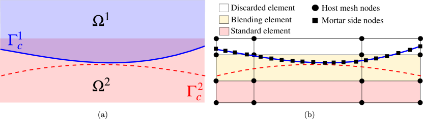
Figure 7: Contact between real surface $\displaystyle\Gamma_{c}^{1}$ and embedded surface $\displaystyle\Gamma^{2}_{c}$: (a) continuum set-up, (b) discretized framework (only surface discretization is shown on the mortar side, whereas the inherent discretization of the embedded surface is not shown on purpose to avoid any confusions).

The concept of coarsening, inspired from [39, 6] and implemented in [1], consists in selecting only few (master) nodes of the mortar surface to carry Lagrange multipliers. Therefore the associated traction field is interpolated over the mortar surface using classical shape functions, with the difference that they span now few elements. Alternatively, one can assign Lagrange multipliers to remaining (slave) mortar nodes and use classical local interpolation shape functions for Lagrange multipliers; however, the values of these slave Lagrange multipliers should be constrained to be a linear combination of Lagrange multipliers of neighbouring master nodes, the associated weights still should be defined by non-local shape functions spanning all the edges which connect the corresponding master nodes. This alternative approach, which is used in this work, can be achieved using multi-point constraints (MPC) for Lagrange DoFs. The concept of coarse-grained interpolation (CGI) is illustrated in Fig. 8. Here, we choose an arbitrary discretized curved mortar surface $\displaystyle\Gamma^{1}_{c}$ which comes in contact with an embedded surface $\displaystyle\Gamma^{2}_{c}$ cutting through blending elements of the non-mortar host mesh $\displaystyle\Omega^{2}$. In this example, on purpose we choose such discretization that mortar nodes (potentially carrying Lagrange multipliers) largely outnumber blending elements. In this situation, the related contact (or tying) interface can be considered over-constrained especially when the mortar side material is considerably more rigid than this of the non-mortar side.

To construct a coarse-grained interpolation, we proceed to the selection of master nodes on the mortar side, which will carry lagrange multipliers. This selection can be guided either by the global or a local mesh density contrast. In the former case, we introduce a global mesh density contrast parameter $\displaystyle m_{c}$ which is the ratio of mortar-side segments $\displaystyle N^{m}$ to the number of blending elements $\displaystyle N^{b}$, i.e. $\displaystyle m_{c}=N^{m}/N^{b}$. For approximately equal discretizations $\displaystyle m_{c}\approx 1$ or coarser discretization of the mortar $\displaystyle m_{c}<1$, the coarse-graining is usually not needed. But for higher density on the mortar side $\displaystyle m_{c}>1$, only few mortar nodes should carry Lagrange multipliers. To characterize it, we introduce a coarse-graining spacing parameter or simply spacing parameter $\displaystyle\kappa$ , which denotes that only every $\displaystyle\kappa$-th mortar node will be assigned as master node [Fig. 8(b)]. The limit case $\displaystyle\kappa=1$, all mortar nodes carry Lagrange multipliers, which corresponds to the standard Lagrange interpolation (SLI). Evidently, such an approach based on the global mesh-density contrast, is expected to perform well only for regularly meshed surfaces and regular size of blending elements. Otherwise, a local approach should be used, in which, for example, one master node per homologue blending element is selected [Fig. 8(b)]. The global approach results in a uniform spacing between master nodes (possibly with an exception of one extremity of the mortar side) and local approach has a potentially variable spacing.

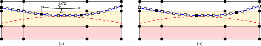
Figure 8: Coarse graining of Lagrange multipliers for an interface with mesh contrast parameter $\displaystyle m_{c}=7$ (the ratio of 21 mortar segments to 3 blending elements): (a) a global approach in which every seventh mortar node is selected as master one and is assigned to carry Lagrange multipliers, (b) local coarse-graining in which only one mortar node per homologue blending element is selected as master.

Let assume that we have a pair of neighbouring master nodes $\displaystyle 1$ and $\displaystyle N$, carrying Lagrange multipliers $\displaystyle\underline{\bm{\lambda}}_{1}$ and $\displaystyle\underline{\bm{\lambda}}_{N}$ and separated by distance $\displaystyle L$, which is the sum of the lengths of segments $\displaystyle L_{i,i+1}$ with $\displaystyle i\in[1,N-1]$ connecting these nodes, i.e. $\displaystyle L=\sum_{i=1}^{N}L_{i,i+1}$. Therefore, within the context of MPC, to interpolate Lagrange multipliers we assign to every slave node $\displaystyle i$ a nominal value of Lagrange multiplier as

$$\tilde{\!\!\,\lambda}_{i}=\lambda_{1}(1-L_{1,i})/L+\lambda_{N}L_{i,N}/L,$$

where $\displaystyle L_{i,j}=\sum_{k=i}^{j-1}L_{i,i+1}$ is the total length of segments connecting nodes $\displaystyle i$ and $\displaystyle j$. Subsequently, the classical local shape functions can be used to interpolate the field of Lagrange multipliers over every segment; this approach is adopted here. Alternatively, a coarse-grained parametrization with normalized parameter $\displaystyle\xi^{CG}$ could be used; it should fulfil the following condition

$$\forall i\in[1,N-1]:\quad\frac{\xi^{CG}_{i+1}-\xi^{CG}_{i}}{L_{i,i+1}}=\mathrm{const},$$

then classical but non-local shape functions can be used to interpolate the field of Lagrange multipliers:

$$\lambda(\xi^{CG})=\lambda^{1}\tilde{\Phi}_{1}(\xi^{CG})+\lambda^{N}\tilde{\Phi}_{2}(\xi^{CG}).$$ (60)

The choice of optimal spacing parameter $\displaystyle\kappa$ was studied in [1]. To summarize the drawn conclusions: (1) the choice of the spacing, which ensures that the distance between master mortar nodes is greater than the average dimension of blending elements, allows to get rid of spurious oscillations; (2) to preserve the accuracy of the solution the $\displaystyle\kappa$ parameter should not be too large.

7.2 Contact patch test

To illustrate the stabilization techniques, a contact patch test shown in Fig. 7 is used, where outer surface $\displaystyle\Gamma_{c}^{1}\subset\partial\Omega^{1}$ comes in contact with an embedded surface $\displaystyle\Gamma_{c}^{2}\subset\Omega^{2}$ (Fig. 9). The classical contact patch test [54, 19] is adjusted to the case of different materials by constraining the normal displacement on lateral sides. A very similar test was presented for mesh tying along straight interfaces in [1], with the only difference that here the developed MorteX contact algorithm is used.

The particular case of softer and coarser host mesh is chosen, as this combination is known to be the most prone to spurious oscillations along the interface [1]. Additionally, the host domain is meshed on purpose with distorted quadrilateral elements in order to obtain a local parametrization that is not aligned with the embedded surface. Linear elastic material properties are used for both the domains $\displaystyle\Omega^{1}$ ($\displaystyle E_{1}=1000$ GPa, $\displaystyle\nu_{1}=0.3$) and $\displaystyle\Omega^{2}$ ($\displaystyle E_{2}=1$ GPa, $\displaystyle\nu_{2}=0.3$). The geometric set-up is illustrated in Fig. 9(a). The discretization for the domains is shown in Fig. 9(b), resulting in a mesh-density contrast $\displaystyle m_{c}\approx 11$. Plane strain formulation is used. A uniform pressure $\displaystyle\sigma_{0}=1$ Pa is applied on the top surface, while the bottom surface is fixed in all directions ($\displaystyle\underline{\bm{u}}=0$) and the lateral sides are constrained in the normal direction $\displaystyle u_{x}=0$ (Fig. 9 (a)). The exact solution for the vertical stress component is a uniform field $\displaystyle\sigma_{yy}=\sigma_{0}$. Fig. 10 shows that the standard Lagrange multiplier interpolation (SLI) exhibits high-amplitude spurious oscillations with errors locally exceeding $\displaystyle 300$ % and spanning many layers of elements in the bulk.

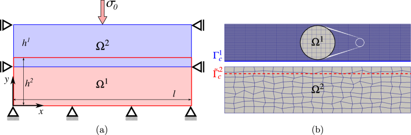
Figure 9: (a) Patch test setup; (b) host mesh has a coarser discretization than the mortar side mesh with the mesh density contrast $\displaystyle m_{c}\approx 12$.

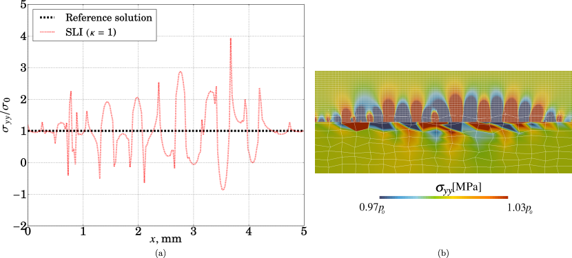
Figure 10: Result of the patch-test in the absence of any stabilisation: (a) $\displaystyle\sigma_{yy}$ along $\displaystyle\Gamma_{c}^{1}$, (b) contour plot of $\displaystyle\sigma_{yy}$.

As we seek to approximate a uniform stress state, a single Lagrange multiplier with a zero order interpolation should be sufficient. Here, however, two Lagrange multipliers are used to demonstrate the effect of coarse-graining interpolation. This interpolation is achieved by assigning Lagrange multipliers to both end nodes of the mortar surface $\displaystyle\Gamma_{c}^{1}$ which act as master nodes for the multi-point constraints, while the nodes lying in-between are the slaves, and the Lagrange multipliers are expressed as a linear combination of the Lagrange multipliers hosted by the master nodes (60). Fig. 11(a) shows that the amplitude of the stress oscillations along the contact interface are significantly reduced ($\displaystyle<1$ %). However, the stresses $\displaystyle\sigma_{yy}$ in the host mesh still exhibit oscillations of amplitude ($\displaystyle\approx 3$ %). This shows that although the CGI scheme allows drastic reduction in stress oscillations, it is not sufficient to recover the reference uniform stress distribution. Surprisingly, the reference field can be recovered if initially quadrilateral blending elements of the host mesh are triangulated. As seen in Fig. 11(b) no visible oscillations are observed in the interface even though this triangulation does not resolve the problem of over-constraining.

Nevertheless, as will be demonstrated below, passing this patch test does not guarantee, in the general case, that using triangular host mesh ensures accurate stress fields near the interface. As was demonstrated in [1] for mesh tying, the considered configuration of the patch test is the only example in which triangulation is sufficient to get rid of spurious oscillations and recover the reference solution. In a more general case, when the interface stress is non-uniform, simple triangulation does allow to obtain accurate solution and is as prone to spurious oscillations as a quadrilateral mesh. Therefore, it could be reasonably thought that the coarse graining should be always combined with the triangulation of blending elements in order to ensure a good performance in any case. However, as was demonstrated in numerous examples in [1], the triangulation can slightly deteriorate the accuracy of the solution. Finally, from the practical point of view, the triangulation of blending elements can be a user-defined option, whereas coarse-grained interpolation is a needed feature as will be shown below on more realistic contact examples.

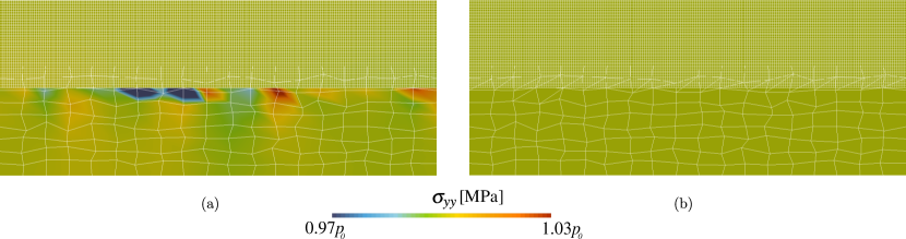
Figure 11: MorteX patch test, stress component $\displaystyle\sigma_{yy}$: (a) coarse-grained interpolation (CGI) with two master nodes assigned on the extremities of the mortar surface; (b) triangulation of blending elements.

8 Numerical examples

In this section, we carefully selected numerical tests to demonstrate the accuracy, the robustness and the efficiency of the method. Linear elements are used in all the examples. All the examples are set-up using both boundary-fitted domains and embedded surfaces, solved within classical mortar and MorteX frameworks, respectively. Both methods were implemented in in-house finite element suite Z-set [12]. In the figures displaying contour stress plots, transparency is used to visually differentiate between the “discarded” (most transparent), “blending” (semi transparent) and “standard” (opaque) elements.

8.1 Frictionless contact of cylinders

As demonstrated in [1] for mesh tying problems, set-up involving a host that is softer and coarser than the patch tend to exhibit spurious interface oscillations as a result of mesh-locking. In order to illustrate the mesh-locking effect within the context of contact problems, we choose the below set-ups for mortar [Fig. 12] and MorteX [Fig. 13]. The problem under consideration is the frictionless Hertzian contact between two infinite cylinders. For the MorteX set-up, the bottom cylinder surface is embedded into a host rectangular domain $\displaystyle\Omega^{2}$. The cylinders are of equal radii $\displaystyle R_{1}=R_{2}=8$ mm. Linear elastic materials are used for both domains $\displaystyle\Omega^{1}$ ($\displaystyle E_{1},\nu_{1}$) and $\displaystyle\Omega^{2}$ ($\displaystyle E_{2},\nu_{2}$). A material contrast is introduced by choosing $\displaystyle E_{1}/E_{2}=100$. The same Poisson ratio of $\displaystyle\nu_{1}=\nu_{2}=0.3$ is used for both the domains. The top cylinder has a finer discretization compared to the bottom cylinder, with the mesh contrast parameter $\displaystyle m_{c}\approx 3$. A vertical displacement $\displaystyle u_{y}=0.005$ mm is applied on the surface of the top cylinder. This results in a total reaction force of $\displaystyle P\approx 0.016512$ N. The bottom surface is fully fixed. The middle point of the top surface is fixed in $\displaystyle x$ direction. For the classical mortar framework contact is enforced between the real-real surface pair ($\displaystyle\Gamma_{c}^{1}/\Gamma_{c}^{2}$), while for MorteX the contact is enforced between the real-virtual surface pair ($\displaystyle\Gamma_{c}^{1}/\tilde{\Gamma}_{c}^{2}$).

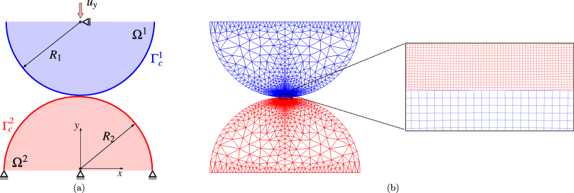
Figure 12: Mortar Hertzian contact: (a) problem set-up and boundary conditions; (b) FE discretization, with mesh contrast parameter $\displaystyle m_{c}\approx 3$ (zoom at the interface mesh).

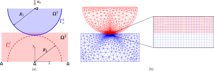
Figure 13: MorteX Hertzian contact: (a) problem set-up and boundary conditions; (b) FE discretization, with mesh contrast parameter $\displaystyle m_{c}\approx 3$ (zoom at the interface mesh).

The analytical solution for this problem is derived from the Hertzian contact formulae for two cylinders, which defines the maximum contact pressure ($\displaystyle p_{0}$), the semi-width of contact zone $\displaystyle a$, and the contact pressure distribution $\displaystyle p$ along the $\displaystyle x$ coordinate [33]:

$$p_{0}=\sqrt{\frac{PE^{*}}{\pi R^{*}}},$$ (61)

$$a=\sqrt{\frac{4PR^{*}}{\pi E^{*}}},$$ (62)

$$p=p_{0}\sqrt{1-\bigg{(}\frac{x}{a}\bigg{)}^{2}}.$$ (63)

In the above equations, the effective elastic modulus $\displaystyle E^{*}$ is defined as

$$E^{*}=\frac{E_{1}E_{2}}{E_{1}(1-\nu_{2}^{2})+E_{2}(1-\nu_{1}^{2})}$$ (64)

and the effective radius $\displaystyle R^{*}$, is evaluated as:

$$R^{*}=\frac{R_{1}R_{2}}{R_{1}+R_{2}}.$$ (65)

Figure 14: Contact stresses ($\displaystyle\lambda_{n},\sigma_{yy}$) for the standard Lagrange multiplier interpolations (SLI): (a) Mortar; (b) MorteX methods.

Using the standard Lagrange multiplier interpolation in which every mortar side node holds a Lagrange multiplier results in spurious oscillations in the stresses [see Fig. 14]. Similar oscillations have been demonstrated in [1] in mesh tying problems. The stabilization technique, coarse graining of Lagrange multiplier interpolations [see Section 7.1], was proved efficient in removing these oscillations on various problem settings for mesh tying problems. We adapt the same stabilization approach for contact problems, to both the mortar and MorteX frameworks. The plots in Fig. 15 show the results obtained by applying the CGI scheme for two values of spacing parameter $\displaystyle\kappa=2,3$ [see Section 7.1]. The amplitude of spurious oscillations are reduced for $\displaystyle\kappa=2$ ($\displaystyle\kappa<m_{c}$) and they are almost eliminated for $\displaystyle\kappa=3$ ($\displaystyle\kappa=m_{c}$), enabling an accurate representation of the analytical contact pressure distribution, only a small perturbation near edges of the contact zone is persisting. The results corroborate the facts established by the patch and Eshelby tests [1], concerning the minimum value that $\displaystyle\kappa$ needs to take for minimizing the effect of mesh-locking ($\displaystyle\kappa\approx m_{c}$). Note that the change in vertical stress in the MorteX framework on the non-mortar side is simply a visualization issue due to inappropriate construction of contour plots in selectively integrated elements .

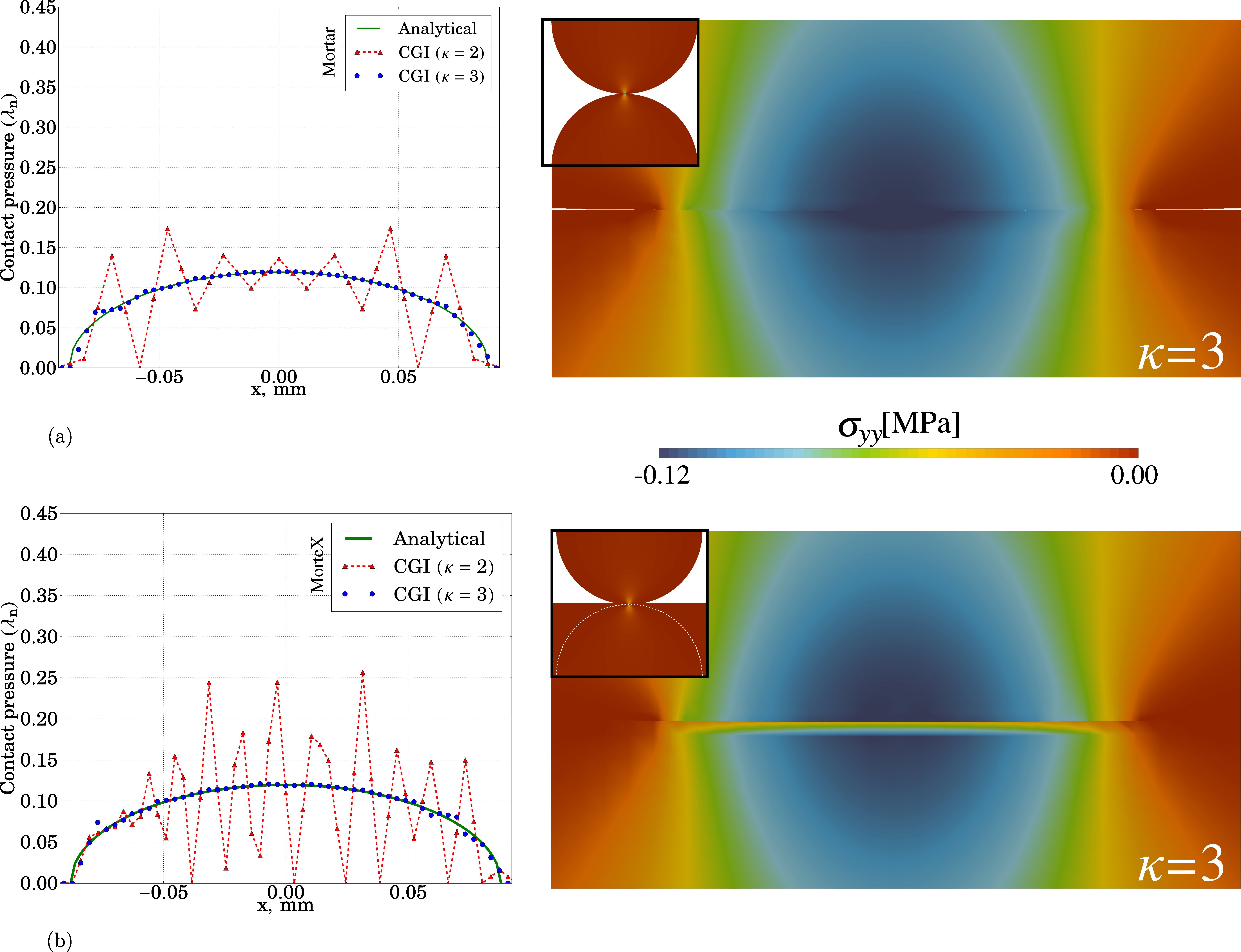
Figure 15: Contact stresses ($\displaystyle\lambda_{n},\sigma_{yy}$) for the coarse grained Lagrange multiplier interpolations (CGI): (a) Mortar; (b) MorteX methods.

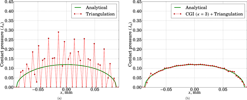
Figure 16: Contact tractions ($\displaystyle\lambda_{n}$) for the MorteX method (a) only triangulation of blending elements; (b) triangulation coupled with the CGI ($\displaystyle\kappa=3$).

For the MorteX method, we additionally test the triangulation of blending elements. As seen from Fig. 16, the triangulation of blending elements reduces the amplitude of oscillations (compared to Fig. 14), which however remain significant. However, when coupled with the CGI stabilization, they do not deteriorate the quality of the solution.

8.2 Frictional contact of cylinders

A set-up similar to the frictionless case [Fig. 13(a)] is considered for the frictional contact. The Coulomb’s friction law is used with the coefficient of friction $\displaystyle\mu=0.2$. The same linear elastic material is assigned to the two cylinders with $\displaystyle E=200$ MPa and $\displaystyle\nu=0.3$. Both cylinders are discretized ensuring equal meshes densities ($\displaystyle m_{c}\approx 1$). This test was also considered in [58, 26]. In the first load sequence, a vertical displacement $\displaystyle u_{y}=0.182$ mm is applied on the top surface of the upper cylinder in 100 load steps, which results in a total reaction force of $\displaystyle P\approx 10.0$ N ($\displaystyle p_{0}\approx 0.625$ N/mm). This is followed by a second sequence of loading where a horizontal displacement $\displaystyle u_{y}=0.03$ mm is applied in 100 load steps. This results in a total reaction force of $\displaystyle Q\approx 0.936$ N ($\displaystyle q_{0}\approx 0.05851$ N/mm). The bottom surface of the lower cylinder is fixed throughout the simulation. The contact pressure profile $\displaystyle p(x)$ and the contact semi-width $\displaystyle a$ are still given by Eqs. (63)-(62).

According to the analytical solution [33], the contact zone is divided into a stick zone in the central area $\displaystyle|x|\leq c$ and two peripheral slip regions $\displaystyle c<|x|\leq a$ , where the semi-width of the stick zone is given by:

$$c=a\sqrt{1-\frac{q_{0}}{\mu p_{0}}}.$$ (66)

The tangential traction $\displaystyle p_{\tau}$ is given as:

$$p_{\tau}(x)=\begin{cases}\quad\displaystyle\mu\frac{4Rp_{0}}{\pi a^{2}}(\sqrt{a^{2}-x^{2}}-\sqrt{c^{2}-x^{2}})&,\mbox{if}\,|x|\leq c;\\[12.0pt] \quad\displaystyle\mu\frac{4Rp_{0}}{\pi a^{2}}(\sqrt{a^{2}-x^{2}})&,\mbox{if}\,c<|x|\leq a;\\ \quad 0&,\mbox{elsewhere.}\end{cases}$$ (67)

Figure 17: Contour stress plots $\displaystyle\sigma_{yy}$, $\displaystyle\sigma_{xy}$ for results obtained by Mortar method.

Figure 18: Contour stress plots $\displaystyle\sigma_{yy}$, $\displaystyle\sigma_{xy}$ for results obtained by MorteX method.

Fig. 17 and 18 show the contour stress plots for $\displaystyle\sigma_{yy}$ and $\displaystyle\sigma_{xy}$ at the end of the second load sequence, obtained with Mortar and MorteX methods, respectively. The results obtained by the Mortar and MorteX methods are very similar to each other, and provide a good approximation of the analytical solution in terms of contact tractions [see Fig. 19].

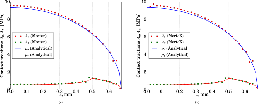
Figure 19: Normal and tangential contact tractions: (a) Mortar; (b) MorteX methods.

8.3 Ironing a wavy surface

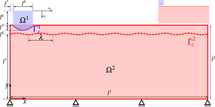
Figure 20: MorteX frictionless ironing of wavy surface set-up, equivalent Mortar set-up (inset).

In this example we consider a frictionless sliding contact between an elastic slider and an elastic wavy substrate [see Fig. 20]. Within the MorteX framework, a discretized surface $\displaystyle\Gamma_{c}^{1}$ comes in contact and slides along a virtual surface $\displaystyle\tilde{\Gamma}_{c}^{2}$ embedded inside a rectangular block. The slider and substrate are meshed with a comparable mesh density ($\displaystyle m_{c}\approx 1$). The geometric dimensions used are: $\displaystyle l^{1}=12,\,l^{2}=4.5,\,l^{3}=4,\,l^{4}=0.2,\,l^{5}=0.3,\,l^{6}=0.9,\,l^{7}=0.2,\,l^{8}=1.2$ (all the length dimension are in mm). The wavy surface is described by $\displaystyle y(x)=l^{3}+\Delta\sin(2\pi x/\lambda)$, with $\displaystyle\lambda=1.5$ mm and $\displaystyle\Delta=0.05$ mm. Both solids are made of the same material: Young’s modulus $\displaystyle E=100$ GPa and Poisson’s ratio $\displaystyle\nu=0.3$. A vertical displacement of $\displaystyle u_{y}=-0.75$ mm is applied on the top of the slider within first 20 load steps ($\displaystyle t\,\in[0,1]$) while the horizontal displacement of the same boundary is kept zero. During the following sequence ($\displaystyle t\,\in[1,2]$), the vertical displacement is maintained and the horizontal displacement of $\displaystyle u_{x}=10$ mm is applied in 100 load steps. The bottom surface of the rectangular block is fixed throughout the simulation.

For the sake of comparison, the same problem is also solved within the classical mortar contact formulation, in which the contact occurs between two surfaces explicitly represented by body-fitted meshes [see Fig. 20, inset]. The contour plots of stresses $\displaystyle\sigma_{yy}$, at $\displaystyle t=1.0,2.0$ seconds, for both the Mortar and MorteX methods are shown in Fig. 21-22. These fields are very smooth and indistinguishable by naked eye. The normalized contact tractions ($\displaystyle\lambda_{n}/E$) and the displacements in $\displaystyle y$-direction ($\displaystyle u_{y}$) along the real surface $\displaystyle\Gamma_{c}^{1}$ are compared between the two methods. In order to quantify the difference between two solutions we use $\displaystyle L^{2}$ norm of displacement and contact traction difference as below:
$$E_{r}(u_{y})=\frac{||u_{y}^{\mbox{\tiny Mortar}}-u_{y}^{\mbox{\tiny MorteX}}||_{L^{2}(\Gamma_{c}^{1})}}{||u_{y}^{\mbox{\tiny Mortar}}||_{L^{2}(\Gamma_{c}^{1})}},$$ (68) $$E_{r}(\lambda_{n})=\frac{||\lambda_{n}^{\mbox{\tiny Mortar}}-\lambda_{n}^{\mbox{\tiny MorteX}}||_{L^{2}(\Gamma_{c}^{1})}}{||\lambda_{n}^{\mbox{\tiny Mortar}}||_{L^{2}(\Gamma_{c}^{1})}}.$$ (69) where the norm is computed as $\displaystyle\left\|f(x)-g(x)\right\|_{L^{2}(\Gamma_{g}^{1})}=\sqrt{\frac{1}{N}\sum_{i=1}^{N}\left[f(x_{i})-g(x_{i})\right]^{2}}$, where $\displaystyle x_{i}\in[0,L]$ are the $\displaystyle x$-coordinates of mortar nodes $\displaystyle\underline{\bm{x}}_{i}\in\Gamma_{g}^{1}$ in the reference configuration. Negligibly small difference between displacements and tractions obtained by the two methods [see Fig. 23] reflects a comparable accuracy the MorteX framework compared to the classical Mortar method.

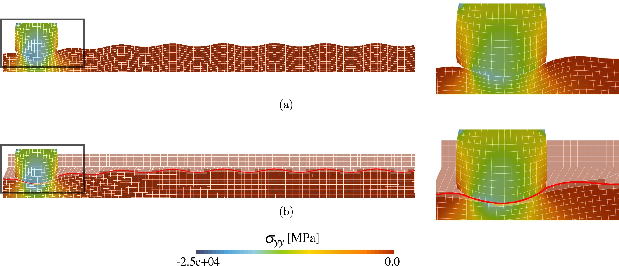
Figure 21: $\displaystyle\sigma_{yy}$ contour plots at $\displaystyle t=1$ s (a) Mortar; (b) MorteX methods.

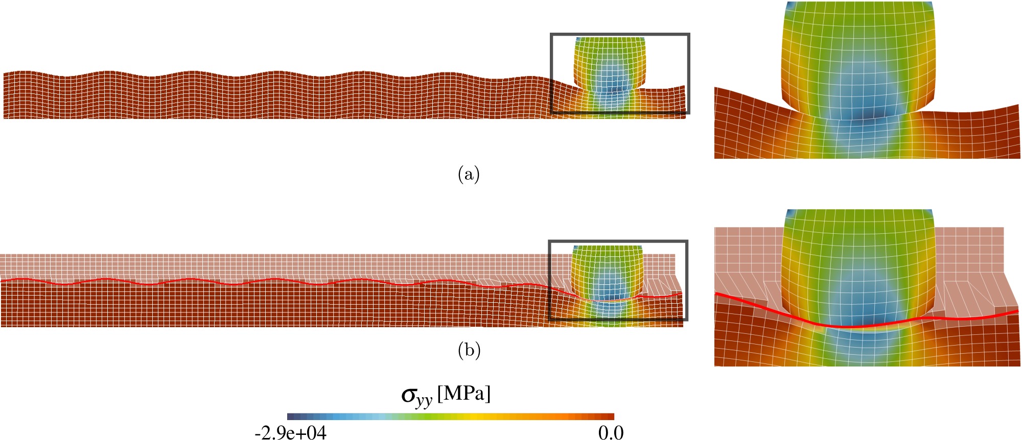
Figure 22: $\displaystyle\sigma_{yy}$ contour plots at $\displaystyle t=2$ s (a) Mortar; (b) MorteX methods.

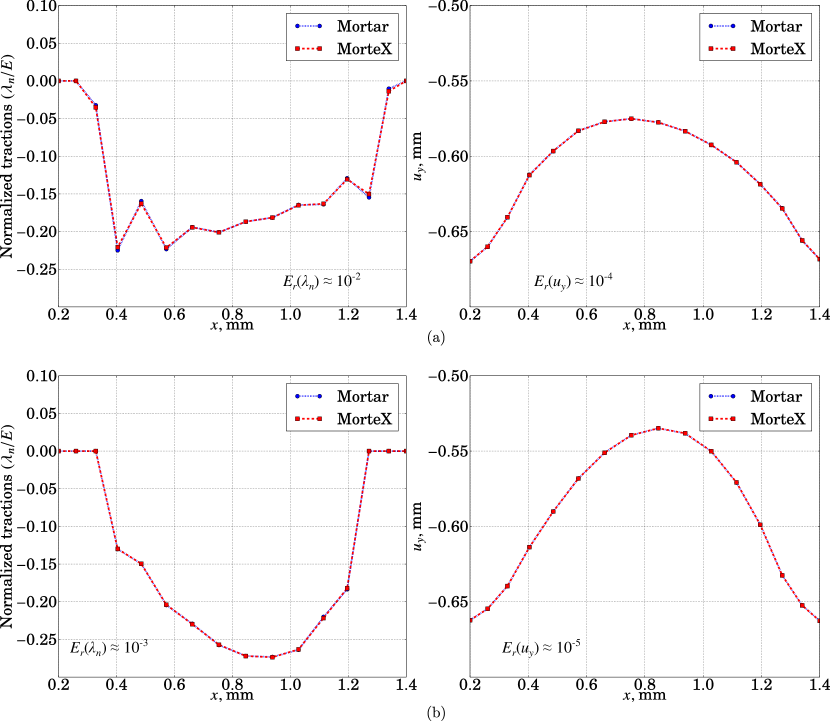
Figure 23: Comparison of normalized contact tractions ($\displaystyle\lambda_{n}/E$) and displacements ($\displaystyle u_{y}$) along slider surface $\displaystyle\Gamma_{c}^{1}$: (a) $\displaystyle t=1$ s; (b) $\displaystyle t=2$ s; associated norms of difference between displacements and pressures obtained by the MorteX and Mortar methods are also shown.

8.4 Frictional shallow ironing

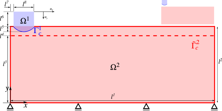
Figure 24: MorteX frictional ironing set-up, equivalent Mortar set-up (inset).

Here we consider the same geometrical set-up as in the previous example (Section 8.3), but here the virtual surface $\displaystyle\tilde{\Gamma}_{c}^{2}$ embedded into the host domain $\displaystyle\Omega^{2}$ is flat [see Fig. 24]. The slider and substrate properties are respectively $\displaystyle E_{1}=68.96$ MPa, $\displaystyle\nu_{1}=0.32$ and $\displaystyle E_{2}=6.896$ MPa, $\displaystyle\nu_{1}=0.32$ ($\displaystyle E_{1}/E_{2}=10$). In addition, the slider has a finer mesh than the substrate: so that the mesh contrast is $\displaystyle m_{c}\approx 3$. A coefficient of friction $\displaystyle\mu=0.3$ is used. The contrast in material and mesh density is introduced purposefully to better illustrate the manifestation of the mesh locking phenomenon. A vertical displacement of $\displaystyle u_{y}=-0.75$ mm is applied on the top of the slider within the first 50 load steps ($\displaystyle t\,\in[0,1]$), while the horizontal displacement of the same boundary is kept zero. During the following sequence ($\displaystyle t\,\in[1,2]$), the vertical displacement is maintained and the horizontal displacement of $\displaystyle u_{x}=10$ mm is applied in 500 load steps. The bottom surface of the rectangular block is fixed in all directions throughout the simulation.

Fig. 25, shows the oscillation in the stress field $\displaystyle\sigma_{yy}$ for the standard Lagrange multiplier interpolations, both in the context of Mortar and MorteX. These results suffer from spurious oscillations. Similar to the Hertzian contact problem setting in Section 8.1, we use the coarse grained Lagrange multiplier interpolations to both the Mortar and MorteX formulations. It results in a reduced amplitude of oscillations, as seen in Fig. 26 and 27 where the contact tractions are presented for different coarse grain spacing parameter $\displaystyle\kappa$. A good agreement between the Lagrange multiplier field $\displaystyle\lambda_{n}$ and hence the reaction forces ($\displaystyle R_{x},R_{y}$) on the slider for the Mortar and MorteX methods can bee seen in Fig. 28. In this example, the applicability of CGI for Lagrange multipliers is once again proved efficient for both the MorteX and for the classical Mortar frameworks.

Figure 25: Standard Lagrange multiplier space ($\displaystyle\kappa=1$), $\displaystyle\sigma_{yy}$ contour plots at $\displaystyle t=2$ seconds (a) Mortar; (b) MorteX methods.

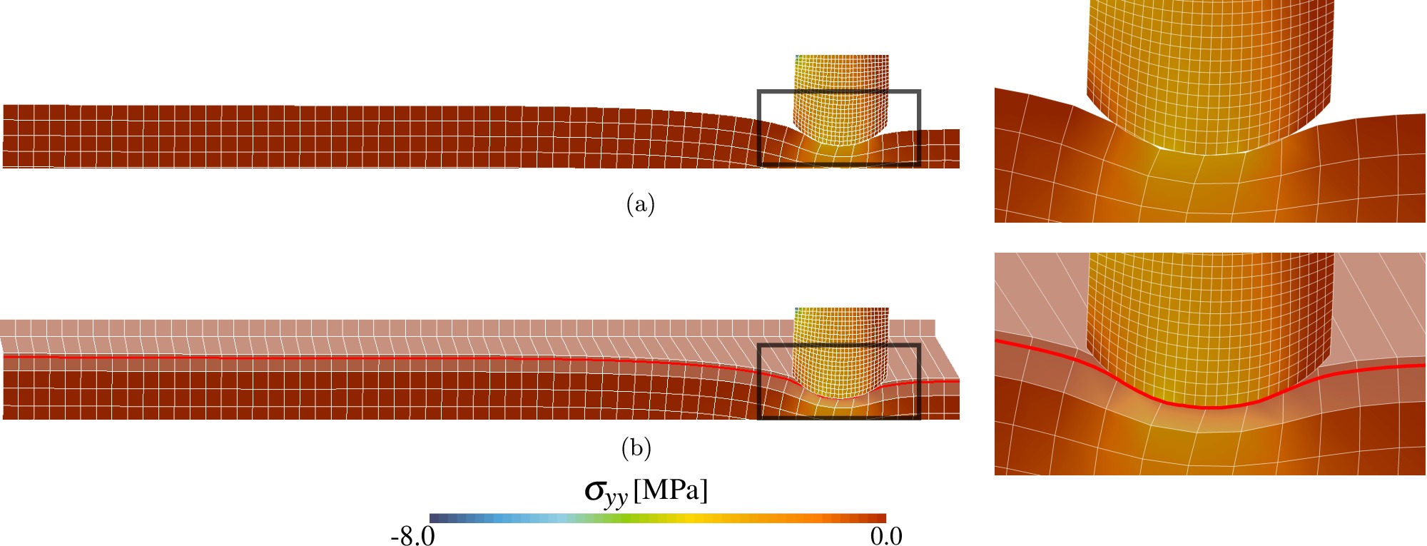
Figure 26: Coarse grained Lagrange multiplier space ($\displaystyle\kappa=3$), $\displaystyle\sigma_{yy}$ contour plots at $\displaystyle t=2$ seconds (a) Mortar; (b) MorteX methods.

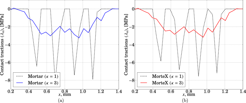
Figure 27: Comparison of $\displaystyle\lambda_{n}$ at nodes along $\displaystyle\Gamma_{c}^{1}$ for $\displaystyle\kappa=1$ and $\displaystyle\kappa=3$: (a) Mortar; (b) MorteX methods at time $\displaystyle t=2$ s.

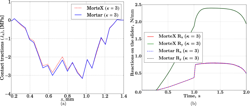
Figure 28: Comparison of Mortar and MorteX methods for CGI with $\displaystyle\kappa=3$: (a) contact tractions $\displaystyle\lambda_{n}$ along $\displaystyle\Gamma_{c}^{1}$; (b) reaction forces in $\displaystyle x$ and $\displaystyle y$ along the top surface of the slider.

9 Concluding remarks

The MorteX framework combining the selective integration from the X-FEM and accurate handling of contact constraints between a boundary fitted and embedded surfaces is developed for the two-dimensional case. The use of the monolithic augmented Lagrangian method renders the constrained optimization problem (resulting from frictional contact) to a fully unconstrained one and ensures a robust convergence because of the resuting smoothed functional which does not require the use of active set strategy common to the method of Lagrange multipliers. Moreover, it presents a comprehensive framework to solve frictional problems without violation of stick constraints inherent to the penalty method. However, for high mesh-density and material contrast, the resulting mixed formulation is shown to be prone to over-constraining of the interface or mesh locking which manifests itself in the form of spurious oscillations. As demonstrated by the classical patch test, these oscillations can be removed if triangular elements are used in the mesh hosting an embedded surface (at least the blending element should be made triangular). However, in real applications, such simple triangulation cannot ensure oscillation-free interface traction fields. To deal with this mesh locking, we adopt here the technique of coarse-grained interpolation of Lagrange multipliers developed in [1]. It consists in assigning Lagrange multipliers only to few mortar-side nodes (master nodes); the choice of the subsampling distance is governed by the relative mesh densities, i.e. the local or global ratio of active mortar nodes per number of active blending elements in contact. The value of Lagrange multipliers of the remaining mortar (slave) nodes is ensured by shape functions spanning few elements. Alternatively, Lagrange multipliers can be assigned to all mortar nodes, but those of the slave nodes can be constrained using multi-point constraints and associated interpolation between master nodes. Such coarse graining cannot ensure a perfect performance of the contact patch test but it enables to reduce the amplitude of spurious oscillations by more than two orders of magnitude for large material contrast (ratio of Young’s moduli equal to 1000) and high mesh density contrast (ratio of the number of mortar nodes per number of blending elements equal to 10). For more realistic contact problems such as frictional contact between two cylinders or shallow ironing, the coarse graining ensures accurate results free of spurious oscillations. Moreover, this coarse-graining is shown to be helpful for the classical mortar method applied to contact problems between boundary fitted surfaces. As demonstrated here, if the material and mesh-density contrast are high between contacting surfaces, spurious oscillations also manifest themselves and can be efficiently removed by the coarse-graining technique. To conclude, we would like to highlight that the good performance of the discretization scheme in the classical contact patch test, where a uniform pressure is transmitted in the contact interface, does not ensure a good performance in a general case. Therefore, it is suggested to extend the contact patch test by applying not only a uniform pressure but also a bending moment [50, 1].

The developed framework should be helpful for wear simulations, where the worn surface can be assumed to be embedded and can propagate inside the bulk mesh due to material loss. The current work is focused on elaborating a methodology to simulate wear within the MorteX framework with an energy-based local wear law. In perspective, this framework is planned to extend to the three-dimensional case. This extension should also involve the possibility to coarse grain Lagrange multipliers and use an appropriate interpolation spanning several mortar faces.

References

- [1] Basava Raju Akula, Julien Vignollet, and Vladislav A. Yastrebov. Stabilized mortex method for mesh tying along embedded interfaces. 2019. submitted.
- [2] Pierre Alart and Alain Curnier. A mixed formulation for frictional contact problems prone to Newton like solution methods. Computer methods in applied mechanics and engineering, 92(3):353–375, 1991.
- [3] Ivo Babuška. The finite element method with Lagrangian multipliers. Numerische Mathematik, 20(3):179–192, 1973.
- [4] Ivo Babuška and Jens M Melenk. The partition of unity method. International journal for numerical methods in engineering, 40(4):727–758, 1997.
- [5] Helio JC Barbosa and Thomas JR Hughes. The finite element method with Lagrange multipliers on the boundary: circumventing the Babuška-Brezzi condition. Computer Methods in Applied Mechanics and Engineering, 85(1):109–128, 1991.
- [6] Éric Béchet, Nicolas Moës, and Barbara Wohlmuth. A stable Lagrange multiplier space for stiff interface conditions within the extended finite element method. International Journal for Numerical Methods in Engineering, 78(8):931–954, 2009.
- [7] F. B. Belgacem, P. Hild, and P. Laborde. The mortar finite element method for contact problems. Mathematical and Computer Modelling, 28(4–8):263 – 271, 1998. Recent Advances in Contact Mechanics.
- [8] F. Ben Belgacem and Y. Maday. A spectral element methodology tuned to parallel implementations. Computer Methods in Applied Mechanics and Engineering, 116(1):59 – 67, 1994.
- [9] Ted Belytschko, Robert Gracie, and Giulio Ventura. A review of extended/generalized finite element methods for material modeling. Modelling and Simulation in Materials Science and Engineering, 17(4):043001, 2009.
- [10] Christine Bernardi. A new nonconforming approach to domain decomposition: the mortar element method. Nonliner Partial Differential Equations and Their Applications, 1994.
- [11] Christine Bernardi, Naïma Debit, and Yvon Maday. Coupling finite element and spectral methods: First results. Mathematics of Computation, 54(189):21–39, 1990.
- [12] J Besson and R Foerch. Large scale object-oriented finite element code design. Computer methods in applied mechanics and engineering, 142(1-2):165–187, 1997.
- [13] Franco Brezzi and Michel Fortin. Mixed and hybrid finite element methods, volume 15. Springer Science & Business Media, 2012.
- [14] Erik Burman and Peter Hansbo. Fictitious domain finite element methods using cut elements: I. A stabilized Lagrange multiplier method. Computer Methods in Applied Mechanics and Engineering, 199(41-44):2680–2686, 2010.
- [15] Federico José Cavalieri and Alberto Cardona. Numerical solution of frictional contact problems based on a mortar algorithm with an augmented lagrangian technique. Multibody System Dynamics, 35(4):353–375, 2015.
- [16] Pedro Diez, Régis Cottereau, and Sergio Zlotnik. A stable extended FEM formulation for multi-phase problems enforcing the accuracy of the fluxes through Lagrange multipliers. International Journal for Numerical Methods in Engineering, 96(5):303–322, 2013.
- [17] John Dolbow, Nicolas Moës, and Ted Belytschko. An extended finite element method for modeling crack growth with frictional contact. Computer methods in applied Mechanics and engineering, 190(51-52):6825–6846, 2001.
- [18] John Everett Dolbow. An extended finite element method with discontinuous enrichment for applied mechanics. Northwestern university, 1999.
- [19] Nagi El-Abbasi and Klaus-Jürgen Bathe. Stability and patch test performance of contact discretizations and a new solution algorithm. Computers & Structures, 79(16):1473–1486, 2001.
- [20] Thomas Elguedj, Anthony Gravouil, and Alain Combescure. A mixed augmented Lagrangian-extended finite element method for modelling elastic–plastic fatigue crack growth with unilateral contact. International Journal for Numerical Methods in Engineering, 71(13):1569–1597, 2007.
- [21] Sonia Fernández-Méndez and Antonio Huerta. Imposing essential boundary conditions in mesh-free methods. Computer methods in applied mechanics and engineering, 193(12-14):1257–1275, 2004.
- [22] G Ferté, P Massin, and N Moës. Interface problems with quadratic X-FEM: design of a stable multiplier space and error analysis. International Journal for Numerical Methods in Engineering, 100(11):834–870, 2014.
- [23] Gaetano Fichera. Boundary value problems of elasticity with unilateral constraints. In Linear Theories of Elasticity and Thermoelasticity, pages 391–424. Springer, 1973.
- [24] KA Fischer and P Wriggers. Frictionless 2d contact formulations for finite deformations based on the mortar method. Computational Mechanics, 36(3):226–244, 2005.
- [25] Kathrin A Fischer and Peter Wriggers. Mortar based frictional contact formulation for higher order interpolations using the moving friction cone. Computer methods in applied mechanics and engineering, 195(37):5020–5036, 2006.
- [26] Markus Gitterle, Alexander Popp, Michael W Gee, and Wolfgang A Wall. Finite deformation frictional mortar contact using a semi-smooth Newton method with consistent linearization. International Journal for Numerical Methods in Engineering, 84(5):543–571, 2010.
- [27] Anthony Gravouil, Emilien Pierres, and Marie-Christine Baietto. Stabilized global–local X-FEM for 3d non-planar frictional crack using relevant meshes. International Journal for Numerical Methods in Engineering, 88(13):1449–1475, 2011.
- [28] Sven Gross and Arnold Reusken. An extended pressure finite element space for two-phase incompressible flows with surface tension. Journal of Computational Physics, 224(1):40 – 58, 2007.
- [29] Martin Hautefeuille, Chandrasekhar Annavarapu, and John E Dolbow. Robust imposition of Dirichlet boundary conditions on embedded surfaces. International Journal for Numerical Methods in Engineering, 90(1):40–64, 2012.
- [30] Magnus R Hestenes. Multiplier and gradient methods. Journal of optimization theory and applications, 4(5):303–320, 1969.
- [31] Patrick Hild. Numerical implementation of two nonconforming finite element methods for unilateral contact. Computer Methods in Applied Mechanics and Engineering, 184(1):99–123, 2000.
- [32] H Ji, D Chopp, and JE Dolbow. A hybrid extended finite element/level set method for modeling phase transformations. International Journal for Numerical Methods in Engineering, 54(8):1209–1233, 2002.
- [33] Kenneth Langstreth Johnson. Contact mechanics. Cambridge University Press, 1985.
- [34] AR Khoei and M Nikbakht. Contact friction modeling with the extended finite element method (X-FEM). Journal of materials processing technology, 177(1-3):58–62, 2006.
- [35] N. Kikuchi and J. Oden. Contact Problems in Elasticity. Society for Industrial and Applied Mathematics, 1988.
- [36] Fushen Liu and Ronaldo I Borja. A contact algorithm for frictional crack propagation with the extended finite element method. International Journal for Numerical methods in engineering, 76(10):1489–1512, 2008.
- [37] TW McDevitt and TA Laursen. A mortar-finite element formulation for frictional contact problems. International Journal for Numerical Methods in Engineering, 48(10):1525–1547, 2000.
- [38] Jens M Melenk and Ivo Babuška. The partition of unity finite element method: basic theory and applications. Computer methods in applied mechanics and engineering, 139(1-4):289–314, 1996.
- [39] Nicolas Moës, Eric Béchet, and Matthieu Tourbier. Imposing Dirichlet boundary conditions in the extended finite element method. International Journal for Numerical Methods in Engineering, 67(12):1641–1669, 2006.
- [40] DS Mueller-Hoeppe, P Wriggers, and S Loehnert. Crack face contact for a hexahedral-based XFEM formulation. Computational Mechanics, 49(6):725–734, 2012.
- [41] G. Pietrzak and A. Curnier. Continuum mechanics modelling and augmented Lagrangian formulation of multibody, large deformation frictional contact problems. Computational Plasticity, pages 878–883, 1997.
- [42] G Pietrzak and A Curnier. Large deformation frictional contact mechanics: continuum formulation and augmented Lagrangian treatment. Computer Methods in Applied Mechanics and Engineering, 177(3-4):351–381, 1999.
- [43] Alexander Popp. Mortar methods for computational contact mechanics and general interface problems. PhD Thesis, Technische Universität München, 2012.
- [44] Alexander Popp, Michael W. Gee, and Wolfgang A. Wall. A finite deformation mortar contact formulation using a primal-dual active set strategy. International Journal for Numerical Methods in Engineering, 79(11):1354–1391, September 2009.
- [45] M. J. D. Powell. Algorithms for nonlinear constraints that use lagrangian functions. Mathematical Programming, 14(1):224–248, December 1978.
- [46] Michael A Puso and Tod A Laursen. A mortar segment-to-segment contact method for large deformation solid mechanics. Computer methods in applied mechanics and engineering, 193(6):601–629, 2004.
- [47] Michael A Puso and Tod A Laursen. A mortar segment-to-segment frictional contact method for large deformations. Computer methods in applied mechanics and engineering, 193(45):4891–4913, 2004.
- [48] Aurelia Cuba Ramos, Alejandro M Aragón, Soheil Soghrati, Philippe H Geubelle, and Jean-François Molinari. A new formulation for imposing Dirichlet boundary conditions on non-matching meshes. International Journal for Numerical Methods in Engineering, 103(6):430–444, 2015.
- [49] Rachelle Ribeaucourt, M-C Baietto-Dubourg, and Anthony Gravouil. A new fatigue frictional contact crack propagation model with the coupled X-FEM/LATIN method. Computer Methods in Applied Mechanics and Engineering, 196(33-34):3230–3247, 2007.
- [50] Jessica D Sanders, Tod A Laursen, and Michael A Puso. A Nitsche embedded mesh method. Computational Mechanics, 49(2):243–257, 2012.
- [51] James Albert Sethian. Level set methods and fast marching methods: evolving interfaces in computational geometry, fluid mechanics, computer vision, and materials science, volume 3. Cambridge university press, 1999.
- [52] Natarajan Sukumar and Ted Belytschko. Arbitrary branched and intersecting cracks with the extended finite element method. International Journal for Numerical Methods in Engineering, 48:1741–1760, 2000.
- [53] Natarajan Sukumar, David L Chopp, Nicolas Moës, and Ted Belytschko. Modeling holes and inclusions by level sets in the extended finite-element method. Computer methods in applied mechanics and engineering, 190(46):6183–6200, 2001.
- [54] Robert L Taylor and Panayiotis Papadopoulos. On a patch test for contact problems in two dimensions. Computational methods in nonlinear mechanics, pages 690–702, 1991.
- [55] Barbara I. Wohlmuth. A Mortar Finite Element Method Using Dual Spaces for the Lagrange Multiplier. SIAM J. Numer. Anal., 38(3):989–1012, August 2000.
- [56] Barbara I. Wohlmuth. Discretization Methods and Iterative Solvers Based on Domain Decomposition, volume 17 of Lecture Notes in Computational Science and Engineering. Springer Berlin Heidelberg, Berlin, Heidelberg, 2001.
- [57] Peter Wriggers. Computational contact mechanics. Springer, Berlin, 2nd edition, 2006.
- [58] Bin Yang, Tod A. Laursen, and Xiaonong Meng. Two dimensional mortar contact methods for large deformation frictional sliding. International Journal for Numerical Methods in Engineering, 62(9):1183–1225, March 2005.