Dynamics and control for multi-agent networked systems: a finite difference approach

Abstract.

We analyze the dynamics of multi-agent collective behavior models and its control theoretical properties. We first derive a large population limit to parabolic diffusive equations. We also show that the non-local transport equations commonly derived as the mean-field limit, are subordinated to the first one. In other words, the solution of the non-local transport model can be obtained by a suitable averaging of the diffusive one.

We then address the control problem in the linear setting, linking the multi-agent model with the spatial semi-discretization of parabolic equations. This allows us to use the existing techniques for parabolic control problems in the present setting and derive explicit estimates on the cost of controlling these systems as the number of agents tends to infinity. We obtain precise estimates on the time of control and the size of the controls needed to drive the system to consensus, depending on the size of the population considered.

Our approach, inspired on the existing results for parabolic equations, possibly of fractional type, and in several space dimensions, shows that the formation of consensus may be understood in terms of the underlying diffusion process described by the heat semi-group. In this way, we are able to give precise estimates on the cost of controllability for these systems as the number of agents increases, both in what concerns the needed control time-horizon and the size of the controls.

1. Introduction

1.1. Problem formulation and main results

In the last decades, there has been a tremendous surge of interest among researchers from various disciplines of engineering and science in problems related to multi-agent networked systems. This is partly due to the large spectrum of applications in many different areas including subjects such as consensus ([3, 9, 51]), collective behavior of flocks and swarms ([63, 65, 71, 84]), sensor fusion ([35, 68]), random networks ([38]), synchronization of coupled oscillators ([43, 69, 70]), asynchronous distributed algorithms ([30, 59]), formation control for multi-robot systems ([67, 85]), and dynamic graphs ([60]).

For the description of these phenomena, several mathematical models have been introduced with different levels of complexity. From the viewpoint of each individual, the dynamics of the agents can be described in a microscopic way as a system of ordinary differential equations (ODEs). The challenge is to describe complex behaviors by means of simple and local interaction rules.

One of the prevalent models in collective dynamics is the so-called consensus model ([10, 45]) describing the evolution of opinions which tend to have similar beliefs among close neighbors. In it, each opinion is represented by a quantity $x_{i}\in\mathbb{R}^{d}$, $d\geq 1$, and evolves according to the following equations:

$$\dot{x}_{i}(t)=\sum_{j=1}^{N}a_{i,j}(x_{j}(t)-x_{i}(t)),\;\;\;i=1,\ldots,N.$$ (1.1)

Here, the parameters $a_{i,j}$ mainly describe the interaction between the agents $x_{i}$ and $x_{j}$. In this work, we will consider two types of choices for $a_{i,j}$, generating two different classes of models: the linear networked model, where $a_{i,j}$ are constants, and the nonlinear alignment model in which $a_{i,j}=a(|x_{j}-x_{i}|)$ (the terminology will be made clear in Section 2).

One of the principal aspects of interest in collective behavior models is the limit behavior as the number of agents $N$ tends to infinity. When considering a large amount of individuals, to follow each trajectory separately may become a prohibitive task. To overcome this difficulty, one classical approach is to replace (1.1) with a suitable partial differential equation (PDE). Depending on the type of interactions $a_{i,j}$, this is done with different techniques.

On the one hand, one can employ the so-called graph limit method ([57]) to describe the limit of (1.1) as $N\to+\infty$ by means of non-local diffusive models in the form

$$\partial_{t}x(s,t)=\int_{I}W(s,s_{*})(x(s_{*},t)-x(s,t))\,ds_{*}.$$ (1.2)

When (1.1) is a (linear) networked system, the limit (1.2) is linear as well and the kernel $W(s,s_{*})$ reflects the connectivity of the network and its interaction coefficients $a_{i,j}$.

We anticipate that, as expected, the structure of the network beneath (1.1) is of great relevance when performing the graph limit. This fact is reflected in the form of the limit interaction kernel $W(s,s_{*})$.

Indeed, as we shall see in Section 3, in order not to have a trivial dynamics in (1.2) (that is, $W(s,s_{*})\equiv 0$) the network has to be sufficiently dense, meaning that each agent needs to communicate with a large percentage of the whole population.

This fact is not surprising: if the interactions in the model are very mild, the inclusion of more and more agents into the system deteriorates the communications to a point in which the individuals are nearly disconnected.

For alignment models, the same technique can be applied leading to a nonlinear non-local diffusion model of the form

$$\partial_{t}x(s,t)=\int_{I}a(|x(s_{*},t)-x(s,t)|)(x(s_{*},t)-x(s,t))\,ds_{*}.$$ (1.3)

On the other hand, for alignment models, apart than the graph limit approach leading to (1.3), one can also use a mean-field procedure ([64]) leading to a non-local transport equation

$$\partial_{t}\mu(x,t)=\partial_{x}\left(\mu(x,t)\int_{X}a(|y-x|)(x-y)\mu(y,t)\,dy\right).$$ (1.4)

Our first main objective in the present paper is to explain the relations between these possible limits (1.3) and (1.4). In particular, we will show that there is a subordination relation allowing to obtain (1.4) from (1.3) through an averaging process.

Once this first aspect is fully clarified, we will give a deeper insight to the role of $N$ in collective-behavior models. With this regard, we will show that certain characteristic properties of multi-agent systems are badly behaved when analyzing the infinite-agents dynamics.

For doing that, we first focus on a simple example of the collective behavior systems, related to the spatial discretization of the heat equation. This allows to reinterpret and explain several fundamental properties in a very intuitive and easily comprehensible manner.

We will be particularly concerned with the controllability of (1.1) which, in this context, is interpreted as the possibility of steering the system to a state in which all the agents agree on a common opinion (the so-called consensus state) and to do it in a finite time by means of the action of one control acting on one of the system components.

The second main result of our work will be to provide estimates on the control properties of this system in terms of the number of agents $N$. In particular, we shall realize that the cost of controlling (1.1) in finite time blows up exponentially when $N\to+\infty$. This, of course, means that the corresponding infinite-dimensional averaged non-local dynamics will fail to be controllable in finite time.

Inspired on this example, we can analyze others related to multi-dimensional or fractional heat processes, which allow to build networks in which the (divergent) control properties can be quantified as $N\to+\infty$. We also analyze other networks, not directly linked to parabolic models, in which the connectivity is rather dense.

To simplify the presentation we will mainly be concerned with networks in which the control acts on some of the external nodes. But similar results apply when the network is controlled in some interior nodes/agents, and in particular in the case where the number of controlled nodes preserves a constant ratio with respect to $N$.

The analysis presented in this paper is non-exhaustive. There is plenty to be understood in what concerns the control of systems of the form (1.1). But the approach presented here may be useful to exploit the existing techniques and results on the control of numerical approximations of PDEs in this context, and to orient future efforts.

The rest of this paper is organized as follows. First of all, in Section 1.2 we give a general bibliographical overview of the modeling of many-particle systems. Section 2 provides a deeper insight on collective dynamics. We first clarify the distinction between networked and alignment systems, and we introduce a general discussion on the control properties of consensus models. In Section 3, we describe in detail the mean-field and graph limit processes leading to the non-local transport and diffusive equation (1.4) and (1.2). In addition, we show a subordination principle of the non-local transport equation (1.4) to (1.3), and we briefly discuss the case of second-order models. In Section 4, we show how (1.1) may be related to the finite difference discretization of the heat equation, and we use this for analyzing control properties of collective behavior models with the help of some specific examples. Finally, Section 5 is devoted to some final remarks and open problems.

1.2. Modeling aspects

The dynamics of many-particle systems may be described into three scales: microscopic, mesoscopic (sometimes referred to as kinetic), and macroscopic.

At a microscopic level, relevant models, composed by a limited number of particles, may be described in terms of ODEs as in (1.1). At a mesoscopic and macroscopic level, infinite-dimensional models described by PDEs or integro-differential equations are needed. In the first case, these models describe the evolution of the distribution of particles over a phase space. In the second one, they involve macroscopic observable quantities obtained by weighted moments of the distribution functions.

There is a well-defined subordination among these scales, and there are different approaches for describing it.

In this framework, the most classical results date back to the works of Hilbert [39, 40] who, as an example in his sixth problem on the axiomatization of physics, translated into a mathematical setting the concepts of hydrodynamic limits introduced by Boltzmann and Maxwell some years before.

This seminal approach has then been extended in several directions, with a special concern toward the derivation and qualitative analysis of different kinetic models (see [2, 13, 34]).

In this context, a widely used technique nowadays is the mean-field limit ([33, 73]), which refers to the problem of passing from a particle description to continuum models of Vlasov-type ([4, 12, 17, 18, 24, 64]), namely

$$\partial_{t}f=-{\bf{v}}\cdot\nabla_{x}f+\nabla_{v}\cdot({\bf{a}}[f]f).$$ (1.5)

In particular, in the context of collective behavior models, ${\bf{a}}[f]$ is typically of the form ([37])

$${\bf{a}}[f](x,v,t):=\int_{\mathbb{R}^{2d}}r(x,y)(v-v_{*})f(y,v_{*},t)\,dv_{*}dt,$$

with an inter-particle interaction kernel $r$, and (1.5) is the kinetic equation corresponding to a second-order model, in the same spirit as (1.4) corresponds to (1.1).

Mean-field theory originally arose in physics to describe phase transitions ([44, 82]), and was later extended toward several areas including queueing theory ([1]), computer network performance and game theory ([49]), and epidemic models ([50]).

The term mean-field comes from the fact that the limit equation describes a distribution function of the representative particle which is affected by a kind of averaged version of the interactions.

The strategy is essentially to consider the continuity equation of a representative one-particle distribution, which can be obtained from the BBGKY hierarchy of the Liouville equations.

The principal limitation of the mean-field approach is that it does not allow to treat all those situations in which underneath (1.1) there is a graph structure, because particles are indistinguishable.

Nonetheless, models on graphs are relevant in different applications throughout the natural sciences and technology. Examples range from synchronization of neuronal networks in biology ([48]), to Josephson junctions in physics ([80]), or to transient stability in power networks ([25]).

Hence, in some recent works (see, e.g., [57, 58]) a graph-limit strategy based on seminal results of graph theory ([53, 54]) has been developed.

In the context of the consensus model (1.1), this leads to the non-local diffusive equation (1.2), representing the opinion distribution of an infinite number of individuals over a dense network.

In conclusion, these two general limit approaches, strongly rooted in the historical development of multiscale modeling, that we just introduced above, allow to describe the infinite-agents dynamics of a large spectrum of consensus models.

In the following sections, we will present them in detail and we will clarify their analogies and differences.

2. General overview of consensus models

This section is devoted to a general discussion on some fundamental aspects of the consensus model (1.1) and on its most relevant properties, in particular from a control theoretical perspective.

2.1. Description of the models

Thanks to the development of social media, the dynamics of opinion formation has lately become a hot topic in the scientific community ([5, 6, 81, 86]). A complex network of interactions leads to the emergence of groups with various opinions, and such behavior raises several questions, including how groups are formed and how many of them survive throughout time.

In this work, we focus on the consensus model (1.1). As their name suggests, it is typically employed to describe the opinion formation in a group. In it, the variables of interest represent the different viewpoints of the agents with respect to certain topics and their evolution along time through the influence of the neighboring opinions in the state space.

Let $x_{i}\in\mathbb{R}^{d}$, $d\geq 1$ be the opinion of the $i$-th agent, which evolves according to the equation (1.1):

$$\dot{x}_{i}(t)=\sum_{j=1}^{N}a_{i,j}(x_{j}(t)-x_{i}(t)),\;\;\;i=1,\ldots,N.$$

Note that the nature of the interaction, namely of $a_{i,j}\in\mathbb{R}$, plays a key role. In some models (see [66]) the interactions $a_{i,j}$ are simply assumed to be constants, according to the adjacency matrix of an weighted undirected graph, with nodes $x_{i}$, describing the connections between the agents. In more detail,

$$a_{i,j}:=\begin{cases}a_{j,i}>0,&\textrm{ if }i\neq j\textrm{ and }x_{i}\textrm{ is conncected to }x_{j},\\ 0,&\textrm{ otherwise}.\end{cases}$$ (2.1)

Then, the matrix $A=(a_{i,j})$ is symmetric and it describes the behavior of a network of individuals, which are connected if $a_{i,j}>0$ and disconnected if $a_{i,j}=0$. These are the so-called networked multi-agent models.

In other situations, ([64]), these interactions depend nonlinearly on the difference of opinions among the agents, and can be defined as

$$a_{i,j}=\frac{a(|x_{j}-x_{i}|)}{N}.$$ (2.2)

Here, the function $a:\mathbb{R}_{+}\to\mathbb{R}_{+}$ is the so-called influence function acting on the magnitude of relative opinions $|x_{j}-x_{i}|$, which measures how much the behavior of each agent $x_{i}$ is affected by the presence of $x_{j}$. In what follows, taking inspiration from the work [64], we shall refer to this class of systems as alignment models.

We may immediately notice a substantial difference between the two classes of models presented. Indeed, networked systems are linear while the alignment is necessarily nonlinear since the interaction matrix depends on the contrast of opinions $|x_{j}-x_{i}|$.

In addition, there is another important distinction between these two situations which, however, is not clearly detectable at first glance. In the first case of networked models, the interactions $a_{i,j}$ given by (2.1) are fixed and the connectivity between two agents depends only on their indices, identifying their own position in the network. For the alignment models, instead, the interactions $a_{i,j}$ depend on the mutual difference of opinion between the different agents, $|x_{j}-x_{i}|$, but not explicitly on their indices $i$ and $j$.

2.2. The notion of consensus

For linear consensus models (1.1)-(2.1) we can introduce the matrix notation

$$\dot{\textbf{x}}+L\textbf{x}=0,$$ (2.3)

where $\textbf{x}=(x_{1},\ldots,x_{N})$ and $L=(\ell_{i,j})_{i,j=1}^{N}=D-A$ with

$$A=(a_{i,j})_{i,j=1}^{N}$$

and

$$D=\textrm{diag}(d_{1},\ldots,d_{N}),\;\;\;d_{k}=\sum_{j=1}^{N}a_{k,j}.$$

The matrix $L$ in (2.3) is usually called the Laplacian of the adjacency matrix $A$. Since $A$ is symmetric, it is evident by construction that $L$ is real and symmetric. Besides, it is always positive-semidefinite (which in particular implies the non-negativity of all its eigenvalues), with all the row and column sums vanishing. As a consequence, $L$ always has a zero eigenvalue, whose corresponding eigenvector is $v_{0}=(1,1,\dots,1)^{T}$ (since it satisfies $Lv_{0}=0$).

Therefore, a constant state of the form $\textbf{x}_{eq}=(\bar{x},\ldots,\bar{x})^{T}$ is an equilibrium of system (2.3) for which the mean-opinion

$$\bar{x}:=\frac{1}{N}\sum_{i=1}^{N}x_{i}(0)$$

is time-invariant. Indeed, one can easily check that

$$\frac{1}{N}\sum_{i=1}^{N}\dot{x}_{i}(t) =\frac{1}{N^{2}}\sum_{i,j=1}^{N}a_{i,j}x_{j}(t)-\frac{1}{N^{2}}\sum_{i,j=1}^{N}a_{j,i}x_{i}(t)=0.$$

This equilibrium $\textbf{x}_{eq}$ is a state in which all the agents agree on a common opinion, the so-called consensus state.

It has been observed that large groups of autonomous agents have the tendency to look for some sort of uniform configuration, even when the individuals interact only locally. This is usually referred as self-organization, and the resulting phenomenon is called emergent behavior ([21, 42, 64]). From a mathematical point of view, consensus is then a pattern to which the system tends naturally to be attracted.

When and how consensus emerges from the consensus models (1.1), and what types of communication rules influence their formation are natural questions to be considered. In [66, Section I.D] the authors provide an extended account of these real word applications, including fast consensus in small-worlds ([87]), distributed sensor fusion in sensor networks ([68]), and a nonlinear extension of (1.1) such as the Kuramoto model ([36, 72]).

2.3. Controllability properties of consensus models

When the consensus is not achieved by self-organization, it is natural to ask whether it can be generated by means of an external action. This is the so-called notion of organization via intervention.

We analyze this issue from a control theoretical perspective. We do it in a standard way, by adding the control function as an external action described by some given constant parameters $b_{i,j}$:

$$\dot{x}_{i}(t)=\sum_{j=1}^{N}a_{i,j}(x_{j}(t)-x_{i}(t))+\sum_{j=1}^{M}b_{i,j}u_{j}(t),\;\;\;i=1,\ldots,N.$$ (2.4)

Notice that, following the above presentation, in the linear networked case (2.4) may be rewritten in matrix form as

$$\dot{\textbf{x}}+L\textbf{x}=Bu.$$ (2.5)

In some seminal papers (see, e.g., [66]), the authors proposed controls acting on all the components of the system. While this strategy is certainly effective, in many situations it is not optimal and, in the last years, other more efficient approaches have been introduced: Sparse control strategies, concentrating their action only on a small number of agents at each time (see for instance [14]), and the control through leadership, which consists in looking for a single leader to act on a whole group and steer it to the desired configuration ([29, 83]).

As far as the authors know, the aforementioned methods need the whole time interval $[0,\infty)$ for the opinions $x_{i}$ to form a consensus in an asymptotic manner, the object being to stabilize a specific equilibrium of the system. Besides, this is reflected on the infinite dimensional transport model (1.4), whose stabilization properties have been studied, for instance, in [15, 26, 27].

But it is natural to investigate whether a suitable control strategy can drive the system to consensus in finite time.

For finite-dimensional linear systems of the form (2.5) controllability in finite time is equivalent to the so-called Kalman rank condition:

$$\textrm{rank}[B,LB,\ldots,L^{N-1}B]=N.$$

Note however that this rank condition in itself does not yield any estimate on the cost of controlling the system as the dimension $N\to+\infty$, which will constitute one of the main focuses of this paper. This has been partially done for the non-local diffusion model (1.2) in the special case

$$I=\mathbb{R}\quad\textrm{ and }\quad W(s,s_{*})=c_{\alpha}|s_{*}-s|^{-1-2\alpha},\;\alpha\in(0,1),$$

corresponding to the heat equation with fractional Laplacian (see [7, 62, 79]). Notwithstanding, to the best of our knowledge, analogous results for more general kernels $W(s,s_{*})$ are not available in the literature.

In Section 4, we will give a partial answer to this question, by discussing some specific example of linear networked consensus models (1.1)-(2.1). We will relate these models to spatial semi-discretized parabolic equations and, in this way, we will characterize their controllability properties through well-known results in PDE control theory and its numerical analysis. For simplicity, we will focus there on the case of sparse controls.

Note that the controllability property refers to the possibility of steering the system to any final state. Here we are mainly concerned with the control to the consensus configuration, which is a desirable target whatever $N$ is.

In particular, we will distinguish two situations. In a first moment, we will consider models on a sparse graph, whose infinite agent dynamics (1.2) is trivial (that is, $W(s,s_{*})\equiv 0$). As we will see, in this case the system cannot be controlled to consensus in a uniform, with respect to $N$ manner. We shall prove that, to control the system, either the time of control or the size of controls has to diverge. More precisely, we shall prove that controllability may be achieved:

• When the time of control is of the order of $T\sim N^{2}$, in which case the size of the needed control is independent of $N$.

• When the time $T$ is independent of $N$ but with controls of size that blows-up exponentially as $N\to+\infty$.

This is a consequence of the fact that, in the considered model, the interaction among agents is weak, implying that (1.1) requires either a large time or a very costly control strategy in order to be controlled.

As we shall see, this type of results will be shared by a number of graph models for which the control to consensus cannot be expected to be uniform with respect to $N$.

Secondly, we will focus on non-trivial limit diffusion equations (1.2), with $W(s,s_{*})\not\equiv 0$, for which we may expect that the stronger level of interaction among the agents produces better controllability properties.

Nevertheless, we will see that this is not necessarily the case, because of possible spectral accumulations. To clarify this aspect, we will present a couple of examples of dense graphs that behave differently from a control perspective.

3. Infinite agents dynamics

In this Section, we are interested in the large population limit ($N\to+\infty$) of the consensus model (1.1).

As we anticipated in Section 1.2, for collective dynamics, this is generally addressed either through the mean-field or graph limit approach. We introduce here the main ingredients for these two procedures.

3.1. The mean-field limit of alignment models

We present here in a schematic manner the mean-field procedure applied to nonlinear models ((1.1) with $a_{i,j}$ given by (2.2)). The interested reader may find a more detailed description in [33, 37, 74] and the references therein.

The process works as follows:

Step 1

The starting point is to consider the empirical measure

$$\mu^{N}=\mu^{N}(x,t):=\frac{1}{N}\sum_{i=1}^{N}\delta_{x_{i}(t)}(x),\;\;\;x\in\mathbb{R}^{d},$$ (3.1)

which identifies which portion of agents have an opinion $x$ at time $t$.

Step 2

Secondly, it can be shown that the density function $\mu^{N}$ satisfies the equation

$$\begin{cases}\displaystyle\partial_{t}\mu^{N}(x,t)=\partial_{x}\left(\mu^{N}(x,t)\int_{\mathbb{R}^{d}}a(|y-x|)(x-y)\mu^{N}(y,t)\,dy\right),\\[10.0pt] \mu^{N}(x,0)=\mu^{N}_{0}(x),\quad x\in\mathbb{R}^{d},\;t>0,\end{cases}$$ (3.2)

in which the initial datum $\mu^{N}_{0}(x)$ is determined by (3.1) and the initial data of (1.1).

This is a non-local transport equation in which the presence of the convolution kernel describes how the interactions among the agents during the time evolution of the dynamics mix their opinions, thus influencing the general behavior of the whole group.

Step 3

Let $\mu_{0}\in\mathcal{P}_{c}(\mathbb{R}^{d})$, the space of probability measures with compact support in $\mathbb{R}^{d}$, and denote $d_{1}$ the Wasserstein one-distance (see Definition 2.1 in [16]). If we assume that $\lim_{N\to+\infty}d_{1}(\mu_{0}^{N},\mu_{0})=0$ and the interaction function $a$ is enough regular to ensure some compactness property, then according to Theorem 2.1 and Corollary 2.1 in [16], there exists $\mu\in C([0,+\infty);\mathcal{P}_{c}(\mathbb{R}^{d}))$ satisfying (3.2) such that, for any $T>0$,

$$\lim_{N\to+\infty}\left[\sup_{t\in[0,T]}d_{1}(\mu^{N},\mu)\right]=0.$$

Notice that from the definition of $\mu^{N}$ and the equation (3.2), we are assuming that the agents are indistinguishable since any opinion at $x$ has the same dynamics. Therefore, this limit process is appropriate only in the case (2.2), where the interactions $a_{i,j}$ measure the contrast of opinions, but do not take into account from which agents they originate. This reflects the fact that there is no network structure at the basis of alignment models.

3.2. Role of the underlying networks

As we already mentioned in the previous sections, for the linear networked models we are analyzing, in which $a_{i,j}$ depends on the indices $i$ and $j$ but not on the difference of opinions $|x_{i}-x_{j}|$, the classical mean-field limit process is not suitable anymore. For this reason, the mean-field limit procedure cannot be applied to a networked collective behavior model in which the interactions are given as in (2.1).

To better clarify this key aspect, we present below a simple example which highlights the role of the graph structure underlying consensus models.

Example 3.1.

Consider a linear networked model with three agents, whose equation is given by

$$\dot{\textbf{x}}+L\textbf{x}=0\quad\text{and}\quad L=\left(\begin{matrix}1&-1&0\\ -1&2&-1\\ 0&-1&1\end{matrix}\right).$$

Let $\textbf{x}^{\,1}$ and $\textbf{x}^{\,2}$ be two solutions of this model with initial data $\textbf{x}^{\,1}_{0}=(1,0,-1)$ and $\textbf{x}^{\,2}_{0}=(1,-1,0)$, respectively. Note that they have the same initial density function:

$$\mu^{3}(x,0)=\frac{1}{3}\delta_{-1}(x)+\frac{1}{3}\delta_{0}(x)+\frac{1}{3}\delta_{1}(x).$$

However, their dynamics are not identical. In particular (see also Figure 1),

$$\dot{\textbf{x}}^{\,1}(0)=(-1,0,1),\quad\text{but}\quad\dot{\textbf{x}}^{\,2}(0)=(-2,3,-1).$$

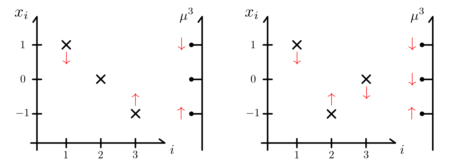
Figure 1. Graphical representation of Example 3.1: two different states $\textbf{x}^{\,1}$ (left) and $\textbf{x}^{\,2}$ (right) generating the same density function $\mu^{3}$.

Example 3.1 shows clearly how, for networked systems, in order to describe completely the dynamics, it is not enough to consider the density of opinions as in model (3.2). Instead, one should adopt a different approach, representing the state as an opinion distribution function whose dynamics will rather be described by a non-local parabolic problem of the form (1.2).

This idea goes back to the pattern formation theory of collective behavior models, for example [46]. Recently its convergence and regularity has been analyzed in [57]. Their relationship is exactly the same as for random variables and their density functions.

This is the basis of the graph limit procedure, which we describe in the next section.

3.3. The graph limit

Recall that (1.1), (2.1) can be seen as a set of $N$ coupled equations on a graph. To analyze the limit when $N\to+\infty$, we adopt the graph limit method presented in [57], where the author combines techniques from the theory of evolution equations and the recent theory of graph limits ([11, 53]) to rigorously justify the possibility of taking the continuum limit for a large class of dynamical models on deterministic graphs.

First of all, let us consider the sub-intervals of $I=[0,1]$ given by

$$I_{i}:=\left[\frac{i-1}{N},\frac{i}{N}\right),\quad i=1,\cdots,N.$$

Let $(x^{N}_{i})_{i=1}^{N}$ be the solution of the consensus model

$$\begin{cases}\displaystyle\dot{x}^{N}_{i}=\frac{1}{N}\sum_{j=1}^{N}a^{N}_{i,j}\psi(x^{N}_{j}-x^{N}_{i}),\\[15.0pt] x^{N}_{i}(0)=g^{N}_{i}\quad i=1,\cdots,N,\end{cases}$$ (3.3)

where $a^{N}_{i,j}=a^{N}_{j,i}$ and $g^{N}_{i}$ are constants and $\psi$ is a Lipschitz continuous function.

Notice that (3.3) contains both the linear dynamics (2.1) and the nonlinear one (2.2). The first one corresponds to take $\psi$ as the identity, while the second one corresponds to $a_{i,j}^{N}=1$ for all $i,j=1,\ldots,N$ and

$$\psi(x_{j}^{N}-x_{i}^{N})=a(|x_{j}^{N}-x_{i}^{N}|)(x_{j}^{N}-x_{i}^{N}).$$

Let $x^{N}(s,t)$ be the opinion-valued distribution function

$$x^{N}(s,t)=\sum_{i=1}^{N}x^{N}_{i}(t)\chi_{I_{i}}(s),\quad s\in I,$$ (3.4)

where $\chi_{I_{i}}$ denotes the characteristic function on $I_{i}$.

Figure 2 shows a diagram representing the relationship between $x_{i}^{N}(t)$ and $x^{N}(s,t)$.

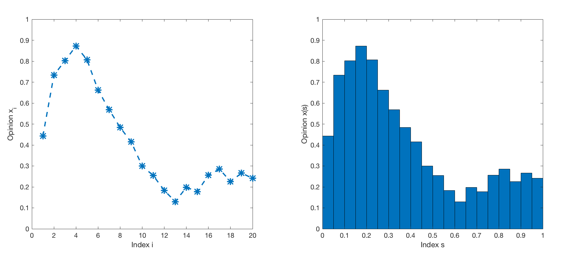
Figure 2. The opinions $(x_{1}^{20},\ldots,x_{20}^{20})$ and their distribution $x^{20}(s,t)$

We have the following result.

Theorem 3.2.

[57] For each $N\in\mathbb{N}$, let $(x^{N}_{i})_{i=1}^{N}$ be the solution of (3.3). Suppose that both the interaction kernel

$$W^{N}(s,s_{*}):=\sum_{i,j=1}^{N}a_{i,j}^{N}\chi_{I_{i}}(s)\chi_{I_{j}}(s_{*}),\quad s,\,s_{*}\in I,\quad W^{N}\in L^{\infty}(I^{2})$$

and the initial datum

$$g^{N}(s):=\sum_{i=1}^{N}g^{N}_{i}\chi_{I_{i}}(s),\quad s\in I,\quad g^{N}\in L^{\infty}(I)$$

are uniformly bounded in $L^{\infty}$ and converge in $L^{2}$ sense to $W$ and $g$, respectively. Then, for every finite $T>0$, the distribution function $x^{N}$ defined in (3.4) converges in $C(0,T;L^{2}(I))$ to the solution $x(s,t)$ of

$$\begin{cases}\displaystyle\partial_{t}x(s,t)=\int_{I}W(s,s_{*})\psi(x(s_{*},t)-x(s,t))\,ds_{*},&s\in I,\;t>0\\ x(s,0)=g(s),&s\in I.\end{cases}$$ (3.5)

Model (3.3) includes a scaling factor $1/N$ which, as we mentioned before, is natural in opinion formation since each agent has to make a compromise of the various opinions of all the other agents in interaction. Hence (see [57]), to ensure that the limit equation (3.5) is not trivial ($W(s,s_{*})\not\equiv 0$) we need a network with the property

$$(\text{\# of nonzero}\leavevmode\nobreak\ a_{i,j}^{N})\sim N^{2}\quad\text{as}\quad N\to+\infty.$$ (3.6)

In what follows, adopting the terminology of [23], we are going to refer as dense graph to a network fulfilling (3.6). On the contrary, if the network does not satisfy this condition, we will call it a sparse graph.

It is worth to mention that (3.6) is compatible with collective dynamics, since the linearization around consensus of the alignment model (2.2) often leads to a dense network. This has been done, e.g., in [14], where the authors obtained local controllability around a consensus point for the linearized alignment model by means of the Kalman’s rank condition.

3.4. An example on a dense graph

To illustrate the importance of the hypothesis (3.6), we describe here the graph limit procedure for a model on a dense graph.

Let us then consider the following system

$$\dot{x}_{i}=\frac{1}{N}\sum_{j=i-\ell}^{i+\ell}(x_{j}-x_{i}),$$ (3.7)

with $\ell=[rN]$, $r\in[0,1]$, where $[rN]$ denotes the closest integer to $rN$.

                                            $\color[rgb]{1,0,0}\bullet\color[rgb]{0,0,0}$$\color[rgb]{1,0,0}\bullet\color[rgb]{0,0,0}$$\color[rgb]{1,0,0}\bullet\color[rgb]{0,0,0}$$\color[rgb]{1,0,0}\bullet\color[rgb]{0,0,0}$$\color[rgb]{1,0,0}\bullet\color[rgb]{0,0,0}$$\color[rgb]{1,0,0}\bullet\color[rgb]{0,0,0}$$\color[rgb]{1,0,0}\bullet\color[rgb]{0,0,0}$$\color[rgb]{1,0,0}\bullet\color[rgb]{0,0,0}$$\color[rgb]{1,0,0}\bullet\color[rgb]{0,0,0}$$\color[rgb]{1,0,0}\bullet\color[rgb]{0,0,0}$$\color[rgb]{1,0,0}\bullet\color[rgb]{0,0,0}$$\color[rgb]{0,0,1}\square\color[rgb]{0,0,0}$$\color[rgb]{0,0,1}\square\color[rgb]{0,0,0}$$\color[rgb]{0,0,1}\square\color[rgb]{0,0,0}$$\color[rgb]{0,0,1}\square\color[rgb]{0,0,0}$$\color[rgb]{0,0,1}\square\color[rgb]{0,0,0}$$\color[rgb]{0,0,1}\square\color[rgb]{0,0,0}$$i-1$……$i-\ell$$i$$i+1$……$i+\ell$

Figure 3. Scheme of the interactions in (3.7). The $i$^th agent communicates with the $j$^th, $j=i-\ell,\ldots,i+\ell$, $\ell=[rN]$.

Recall that (3.7) can be rewritten in the form

$$\dot{\textbf{x}}+L_{r}\textbf{x}=0$$ (3.8)

with $L_{r}=\frac{1}{N}(D_{r}-A_{r})$, where the adjacency matrix $A_{r}$ is

$$A_{r}=(a_{i,j}^{N})_{i,j=1}^{N},\;\;\;a_{i,j}^{N}=\begin{cases}1,&\textrm{if }j=i-\ell,\ldots,i-1,i+1,\ldots,i+\ell,\\ 0,&\textrm{otherwise},\end{cases}$$ (3.9)

and $D_{r}$ is a diagonal matrix indicating the number of connections with each agent in the network, that is

$$D_{r}=\text{diag}(\deg(x_{1}),\ldots,\deg(x_{N}))\;\;\;\deg(x_{i}):=\sum_{j\neq i}|a_{i,j}|.$$

Following the procedure described in Section 3.3, we need to construct an opinion distribution out of the points $x_{i}$.

For doing that, let us denote $\{s_{i}\}_{i=1}^{N}$ a uniform mesh of the space interval $I=[0,1]$. For instance, we set

$$s_{i}=\frac{i}{N}-\frac{1}{2N},\;\;\;i=1,\ldots,N,$$

and consider the intervals

$$I_{i}:=\left[s_{i}-\frac{1}{2N},s_{i}+\frac{1}{2N}\right)=\left[\frac{i-1}{N},\frac{i}{N}\right),$$

so that $\cup_{i=1}^{N}I_{i}=[0,1)$. Out of this, let us define the distribution of phase-values $x^{N}(s,t)$

$$x^{N}(s,t)=\sum_{i=1}^{N}x_{i}^{N}(t)\chi_{I_{i}}(s),\quad s\in I,\;t>0,$$ (3.10)

and assume that $g^{N}:=\sum_{i=1}^{N}x_{i}^{N}(0)\chi_{I_{i}}(s)$ satisfies the assumptions of Theorem 3.2. Then, it is possible to show that (3.10) satisfies the equation

$$\begin{cases}\displaystyle\partial_{t}x^{N}(s,t)=\int_{I}\sum_{i,j=1}^{N}a_{i,j}^{N}\chi_{I_{i}}(s)\chi_{I_{j}}(s_{*})(x^{N}(s_{*},t)-x^{N}(s,t))\,ds_{*},&s\in I,\,t>0\\[15.0pt] \displaystyle x^{N}(s,0)=g^{N}(s),&s\in I.\end{cases}$$

Consider the sequence of the interaction kernels

$$W_{A_{r}}(s,s_{*}):=\sum_{i,j=1}^{N}a_{i,j}^{N}\chi_{I_{i}}(s)\chi_{I_{j}}(s_{*}):I^{2}\to\mathbb{R}.$$

From (3.9) it follows immediately that $|W_{A_{r}}(s,s_{*})|<1$. Moreover, we can readily check that

$$\int_{I^{2}}\Big{(}W_{A_{r}}(s,s_{*})-\chi_{[0,r]}(|s_{*}-s|)\Big{)}^{2}\,ds_{*}ds\leq\frac{4}{N}\to 0,\quad\textrm{ as }N\to+\infty.$$

Hence, $W_{A_{r}}(s,s_{*})$ satisfies the assumptions of Theorem 3.2 and converges in $L^{2}$ to the function $\chi_{[0,r]}(|s_{*}-s|)$. We then conclude that $x^{N}$ converges in $C(0,T;L^{2}(I))$ to some distribution $x$ satisfying the equation

$$\begin{cases}\displaystyle\partial_{t}x(s,t)=\int_{I}\chi_{[0,r]}(|s_{*}-s|)(x(s_{*},t)-x(s,t))\,ds_{*},&s\in I,\,t>0\\[15.0pt] x(s,0)=g(s),&s\in I.\end{cases}$$ (3.11)

3.5. Subordination of the mean-field transport equations

For the sake of completeness, we conclude this section with a brief discussion on the relations between the non-local diffusive models coming from the graph limit of nonlinear aligned systems and the non-local transport ones, obtained through the mean-field limit process ((1.3) and (1.4), respectively).

We start by considering the finite-dimensional nonlinear alignment model

$$\dot{x}_{i}=\frac{1}{N}\sum_{j=1}^{N}a(|x_{j}-x_{i}|)(x_{j}-x_{i}).$$ (3.12)

Recall that (3.12) can be written in the form (3.3) by taking $a_{i,j}^{N}=1$ for all $i,j=1,\ldots,N$ and $\psi(x_{j}-x_{i})=a(|x_{j}-x_{i}|)(x_{j}-x_{i})$.

We may follow the graph limit method (see Theorem3.2), from which we obtain the integro-differential equation

$$\partial_{t}x(s,t)=\int_{I}a\big{(}|x(s_{*},t)-x(s,t)|\big{)}\big{(}x(s_{*},t)-x(s,t)\big{)}\,ds_{*},$$ (3.13)

where $x(s,t)$ is the distribution of the opinion $x_{i}$ over a set $I$ of infinite indices:

$$x(s,t)=\lim_{N\to+\infty}x^{N}(s,t),\quad x^{N}(s,t):=\sum_{i=1}^{N}x_{i}(t)\chi_{I_{i}}(s),\quad s\in I,\;t>0.$$

Note that, this time, the non-local limit (3.13) defines a non-trivial dynamics as soon as $a$ is non-trivial.

On the other hand, the mean-field approach in [64] on the equation (3.12) leads to the following non-local transport PDE:

$$\partial_{t}\mu(x,t)=\nabla_{x}(V[\mu]\mu),\quad\text{where}\quad V[\mu]:=\int_{\mathbb{R}^{d}}a(|x_{*}-x|)(x-x_{*})\mu(x_{*},t)\,dx_{*}.$$ (3.14)

Here $\mu(x,t)$ describes the density of opinions:

$$\mu(x,t)=\lim_{N\to+\infty}\mu^{N}(x,t),\quad\mu^{N}(x,t):=\frac{1}{N}\sum_{i=1}^{N}\delta(x-x_{i}(t)),\quad x\in\mathbb{R}^{d},\;t>0.$$

Although equation (3.13) is parabolic and (3.14) is hyperbolic, there is a relationship among them through the following transformation:

$$\mu(x,t)=\int_{I}\delta(x-x(s,t))ds.$$ (3.15)

Indeed, by employing (3.15), we can firstly rewrite the time derivative $x_{t}$ in terms of $\mu$ as

$$\partial_{t}x(s,t) =\int_{I}a\big{(}|x(s_{*},t)-x(s,t)|\big{)}\big{(}x(s_{*},t)-x(s,t)\big{)}\,ds_{*}$$

$$=\int_{\mathbb{R}^{d}}\mu(x_{*},t)a\big{(}|x_{*}-x(s,t)|\big{)}\big{(}x_{*}-x(s,t)\big{)}\,dx_{*}=-V[\mu](x(s,t)).$$

Then, given a test function $\phi=\phi(x)$, consider the inner product

$$(\mu,\phi):=\int_{\mathbb{R}^{d}}\mu(x,t)\phi(x)\,dx=\int_{I}\phi(x(s,t))\,ds.$$

We have:

$$\frac{d}{dt}(\mu,\phi) =\frac{d}{dt}\int_{I}\phi(x(s,t))\,ds=\int_{I}\big{\langle}x_{t}(s,t),\nabla_{x}\phi(x(s,t))\big{\rangle}\,ds$$

$$=-\int_{I}\big{\langle}V[\mu](x(s,t)),\nabla_{x}\phi(x(s,t))\big{\rangle}\,ds$$

$$=-\int_{\mathbb{R}^{d}}\mu(x,t)\big{\langle}V[\mu](x,t),\nabla_{x}\phi(x)\big{\rangle}\,dx$$

$$=\int_{\mathbb{R}^{d}}\big{\langle}\nabla_{x}(V[\mu](x,t)\mu(x,t)),\phi(x)\big{\rangle}\,dx=\big{(}\nabla_{x}(V[\mu]\mu),\phi\big{)},$$

which constitutes the weak version of (3.14).

Therefore, for the alignment model (1.1), (2.2), the non-local diffusive equation (3.13) includes, in particular, the dynamics of the non-local transport equation (3.14), which is subordinated to the first one.

In the latter, the opinion-valued distribution function is projected into the opinion space to get the density over opinions as in (3.15). During this process, we lose information of the position of the agents.

Finally, note that this subordination principle is significantly different from others such as the Kannai transform (see [28] and the references therein) from the wave to the heat equation.

3.6. Graph limit of second-order models and subordination of mean-field equations

The same methodology that we introduced for the graph limit of (1.1) may be applied also to the study of second-order collective behavior models such as the classical Cucker-Smale system appearing in flock dynamics ([21]), or the second-order Kuramoto equation used for the synchronization of oscillators ([75]).

In particular, the latter one is in the form

$$\ddot{x}_{i}(t)+\dot{x}_{i}(t)=\frac{1}{N}\sum_{j=1}^{N}a_{i,j}(x_{j}(t)-x_{i}(t)),\;\;\;i=1,\ldots,N.$$ (3.16)

In analogy with what we did before, for the sake of completeness, we are going to present here an heuristic description of the process for computing the graph limit of (3.16) and of the subordination to the corresponding mean-field equation. The approach is analogous to the first-order system (1.1). We first need to construct the distribution

$$x^{N}(s,t)=\sum_{i=1}^{N}x_{i}(t)\chi_{I_{i}}(s),\quad s\in I,\;t>0.$$ (3.17)

Then, as $N\to+\infty$, we expect $x^{N}$ to converge to some distribution $x$ satisfying the equation

$$\partial_{tt}x(s,t)+\partial_{t}x(s,t)=\int_{I}W(s,s_{*})(x(s_{*},t)-x(s,t))\,ds_{*},$$ (3.18)

which is a second-order damped wave-like integro-differential equation where, as in (1.2), the kernel $W(s,s_{*})$ inherits the graph structure underneath (3.16).

Notice that, once again, the interactions among the $x_{i}$ in (3.16) generate a non-local term in the limit equation, which this time is in the form of an integral potential.

Besides, also in this case, one can formally establish a relationship among (3.18) and the corresponding mean-field model, by projecting (3.17) into the positions/velocity space. The subordination process works as follows.

Step 1

First of all, we introduce the nonlinear alignment model corresponding to (3.16):

$$\ddot{x}_{i}(t)+\dot{x}_{i}(t)=\frac{1}{N}\sum_{j=1}^{N}a(|x_{j}-x_{i}|)(x_{j}(t)-x_{i}(t)),\;\;\;i=1,\ldots,N.$$ (3.19)

Step 2

By substituting (3.17) into (3.19) we have that, for any $s\in I$ and $t>0$, the distribution $x^{N}(s,t)$ satisfies the nonlinear equation

$$\partial_{tt}x^{N}(s,t)+\partial_{t}x^{N}(s,t)=\int_{I}a\big{(}|x^{N}(s_{*},t)-x^{N}(s,t)|\big{)}\big{(}x^{N}(s_{*},t)-x^{N}(s,t)\big{)}\,ds_{*}.$$ (3.20)

Then, in the same spirit of Theorem 3.2, we may formally see that, as $N\to+\infty$, $x^{N}(s,t)$ converges to a distribution $x(s,t)$ which satisfies the nonlinear non-local wave model

$$\partial_{tt}x(s,t)+\partial_{t}x(s,t)=\int_{I}a\big{(}|x(s_{*},t)-x(s,t)|\big{)}\big{(}x(s_{*},t)-x(s,t)\big{)}\,ds_{*}.$$ (3.21)

Step 3

Through the transformation

$$g(x,v,t)=\int_{I}\delta(x-x(s,t))\delta(v-\partial_{t}x(s,t))ds,$$

with a similar procedure as in the first-order case, from (3.21) we recover the kinetic equation

$$\begin{cases}\partial_{t}g=-v\cdot\nabla_{x}g+\nabla_{v}\cdot\big{(}F[g]g\big{)}\\[5.0pt] \displaystyle F[g]=\int_{V}\Big{[}a(|x_{*}-x|)(x-x_{*})+v\Big{]}g(x_{*},v_{*},t)\,dx_{*}dv_{*}.\end{cases}$$ (3.22)

Moreover, this three-step process is not specific to (3.22), but may be extended to other kinetic models. Nevertheless, we have to stress that this is a merely heuristic procedure, which may be difficult to justify rigorously.

In contrast with the first-order case, the equation being of wave-like form the limit process in Step 2 may be hard to be performed. Indeed, in the present case, in the absence of regularizing effect, passing to the limit in the nonlinear term is not trivial, as it often occurs in nonlinear wave theory.

Nonetheless, despite of the fact that the limit process is purely formal, the subordination of (3.22) to (3.21) is in itself a good indication of the interest of the approach.

4. Dependence of control properties on the number of agents $N$

In this section, we analyze the impact of the number of agents $N$ on the dynamics of the consensus model (1.1). Our principal scope is to discuss to which extent the number of individuals $N$ involved in the model affects its general behavior and control properties.

As we anticipated, this will be done by interpreting (1.1) as semi-discretized parabolic equations and by using classical PDE techniques to identify the role that $N$ plays. This will allow to describe how the time scale and the control cost evolve with respect to $N$.

4.1. From opinion dynamics to semi-discretized PDEs

We start with an example of network dynamics on a sparse graph, which is closely related to the one-dimensional semi-discretized heat equation.

Recall that, according to the discussion at the end of Section 3.3, this case corresponds to a trivial limit dynamics (1.2), in which $W(s,s_{*})=0$.

Let us consider the consensus formation model (1.1), and assume for simplicity that the opinions are described by scalar functions $x_{i}(t)\in\mathbb{R}$, $i=1,\ldots,N$, and that the agents (denoted by the index $i$) are aligned along the same line. In addition, let us define the interactions by

$$a_{i,j}=\begin{cases}1,&\textrm{ if }j=i-1,\,i+1,\\ 0,&\textrm{ otherwise}.\end{cases}$$ (4.1)

In other words, the agent $i$ is communicating only with the left and right neighbor $i-1$ and $i+1$, meaning that the graph describing these interactions has a very simple structure in which all the nodes are aligned on the same line and ordered in a chain (see Figure (4)).

                                            $\color[rgb]{1,0,0}\bullet\color[rgb]{0,0,0}$$\color[rgb]{1,0,0}\bullet\color[rgb]{0,0,0}$$\color[rgb]{1,0,0}\bullet\color[rgb]{0,0,0}$$\color[rgb]{1,0,0}\bullet\color[rgb]{0,0,0}$$\color[rgb]{1,0,0}\bullet\color[rgb]{0,0,0}$$\color[rgb]{1,0,0}\bullet\color[rgb]{0,0,0}$$\color[rgb]{1,0,0}\bullet\color[rgb]{0,0,0}$$\color[rgb]{1,0,0}\bullet\color[rgb]{0,0,0}$$\color[rgb]{1,0,0}\bullet\color[rgb]{0,0,0}$$\color[rgb]{1,0,0}\bullet\color[rgb]{0,0,0}$$\color[rgb]{1,0,0}\bullet\color[rgb]{0,0,0}$$\color[rgb]{0,0,1}\square\color[rgb]{0,0,0}$$\color[rgb]{0,0,1}\square\color[rgb]{0,0,0}$$1$$2$$i-1$$i$$i+1$$N$…………

Figure 4. Scheme of the interactions corresponding to (4.1). The agent $i$ communicates only with $j$, $j=i\pm 1$.

To some extent, one can relate $i=1,\ldots,N$ with the indices of the points of a uniform mesh discretizing the real line or a sub-interval of it.

In view of the structure of the interaction matrix (4.1), if we denote $\textbf{x}:=(x_{1},\ldots,x_{N})^{T}$, we can easily see that system (1.1) may be written in matrix notation as

$$\dot{\textbf{x}}+L\textbf{x}=0$$ (4.2)

where the Laplacian matrix $L$ is given by

$$L=\left(\begin{matrix}1&-1&0&\ldots&\ldots&0\\ -1&2&-1&\ldots&\ldots&0\\ \vdots&&\ddots&&&\vdots\\ \vdots&&&\ddots&&\vdots\\ 0&\ldots&\ldots&-1&2&-1\\ 0&\ldots&\ldots&\ldots&-1&1\end{matrix}\right)_{N\times N},$$ (4.3)

uniformly bounded on $N$.

There is a clear similarity between (4.2)-(4.3) and the classical finite difference discretization of the one-dimensional heat equation with homogeneous Neumann boundary condition on a interval $I\subset\mathbb{R}$, say $[0,1]$, which is given by

$$\dot{\textbf{x}}+D\textbf{x}=0$$ (4.4)

and

$$D=N^{2}L.$$ (4.5)

In (4.4), we immediately recognize the finite difference semi-discretization of the one-dimensional heat equation. Accordingly, (4.2) can be seen as a finite-difference discretization of the heat equation

$$u_{t}-\sigma u_{xx}=0,$$ (4.6)

with diffusivity $\sigma=\sigma(N):=N^{-2}$.

The heat equation is one of the paradigmatic models for which the existing PDE control theory is rather complete (see [28, 90]). In the present one-dimensional setting the heat equation is null-controllable in any positive time by means of controls acting on the boundary or in interior measurable sets with positive measure. But, of course, the fact that the diffusivity $\sigma(N)=N^{-2}$ vanishes asymptotically has a significant impact on the cost of controlling the system. These properties are inherited by the finite difference semi-discretized models ([89]).

Figure 5. Solution of (4.4) (left) and (4.2) (right) on the time interval $[0,T]$. with $T=0.2s$ and $N=50$.

Systems (4.2) and (4.4) are equivalent up to a change of variables of time-scale $t\mapsto\sigma(N)t=N^{-2}t$:

$$\dot{\textbf{x}}+D\textbf{x}=0,\;\;\;t\in[0,T/N^{2}].$$ (4.7)

A standard way of characterizing controllability properties is through the control cost which, roughly speaking, measures how expensive is the control strategy that one adopts to steer any given initial datum to consensus in a given finite time.

In the finite-dimensional context, the classical Kalman’s condition assures that models (4.2) and (4.4) can be controlled by acting only on one of their components. Besides, the results in [90] show that the cost of controlling (4.2) is of the order of $\exp(CN^{2}/T)$. This means that to control the system with controls uniformly bounded on $N$ one needs to take a control time of the order of $T\sim N^{2}$.

If instead the time horizon $T$ is fixed, independent of $N$, then the cost of controlling system (4.2) increases exponentially: $c(T)\sim\exp(CN^{2}/T)$.

This discussion may be summarized in the following result.

Proposition 4.1.

Let us consider the following control problem associated to (4.2):

$$\dot{\textbf{x}}+L\textbf{x}=B\bf{u},$$ (4.8)

with $L$ given by (4.3) and

$$B=(1,0,\ldots,0)^{T}.$$ (4.9)

The controllability properties of (4.8) can be characterized in terms of the number of agents $N$ in the following way:

1. When the time of control is of the order of $T\sim N^{2}$, controllability to consensus is achievable by acting only on one agent with a control uniformly bounded on $N$.

2. When the time $T$ is independent of $N$, controllability to consensus requires controls of size that blows-up exponentially as $N\to+\infty$.

Notice that the choice of $B$ in Proposition 4.1 corresponds to controlling the network only through one control acting on the agent placed in one of the extremes of it. Nevertheless, the same result would be true in the context of interior control acting on all agents $j$ so that $j/N$ lies in a given sub-interval $(a,b)$ of the network, corresponding to a $N\times j$ control matrix $B$ in the form

$$B=(0,I_{j},0)^{T},$$ (4.10)

where $I_{j}$ indicates the $j\times j$ identity matrix.

In fact the network in which the control acts in all nodes $j$ such that $j/N$ belongs to $(a,b)$ can be seen as two networks, one to the left of $a$, and the other one to the right of $b$, connected by the intermediate control zone $(a,b)$, so that each of them is controlled in the corresponding end-point $a$ or $b$.

The bad behavior of (4.2) in terms of controllability as $N\to+\infty$ can be further explained through the analysis of the spectrum of (4.3).

Following the classical methodology presented in [41, Chapter 9, Section 1.1], we can easily compute the eigenvalues of (4.3) and (4.5), which are given respectively by

$$\lambda_{k}^{L}=\lambda_{k}^{L}(N):=4\sin^{2}\left(\frac{\pi(k-1)}{2N}\right),\;\;\;k=1,\ldots,N$$ (4.11)

and

$$\lambda_{k}^{D}=\lambda_{k}^{D}(N)=N^{2}\lambda_{k}^{L}(N),\;\;\;k=1,\ldots,N.$$ (4.12)

The systems under consideration have a spectrum composed by $N$ real eigenvalues. We are interested here in their control properties as $N$ tends to infinity. To address this we make use of the existing theory of families of dynamical systems that can be represented in Fourier series by a sequence of real exponential, as it occurs in the context parabolic equations. When the spectrum of the system is given by real eigenvalues $\{\lambda_{k}\}_{k\geq 1}$, the controllability of the corresponding parabolic dynamics requires the following two properties to hold:

$$\textrm{1. There exists a constant }\gamma>0\textrm{ such that }\lambda_{k+1}-\lambda_{k}\geq\gamma\textrm{ for all }k\geq 1.$$

$$\textrm{2. The sum }\sum_{\underset{\lambda_{k}\neq 0}{k\geq 1}}\lambda_{k}^{-1}\textrm{ is finite}.$$ (4.13)

In this paper we consider systems depending on the parameter $N$. Thus, the spectrum also depends on $N$. But it is well known (see [90]) that the corresponding systems are uniformly controllable provided the former gap and summability conditions are uniform on the index $N$. Here uniformity means that, for a fixed initial datum (or a family of data converging to a given datum as $N$ tends to infinity) and for a fixed consensus target and a time horizon $T$, the controls remain uniformly bounded as $N$ tends to infinity. The families of eigenvalues under consideration are finite, consisting on $N$ eigenvalues. They can be extended to an infinite sequence by simply setting $\lambda_{j}=j^{2}$ for $j\geq N+1$.

It is easy to see that (4.1) are satisfied uniformly by the eigenvalues (4.12) of the semi-discrete heat equation (4.4), but not by the ones of the consensus model (4.2) (see also Figure 6).

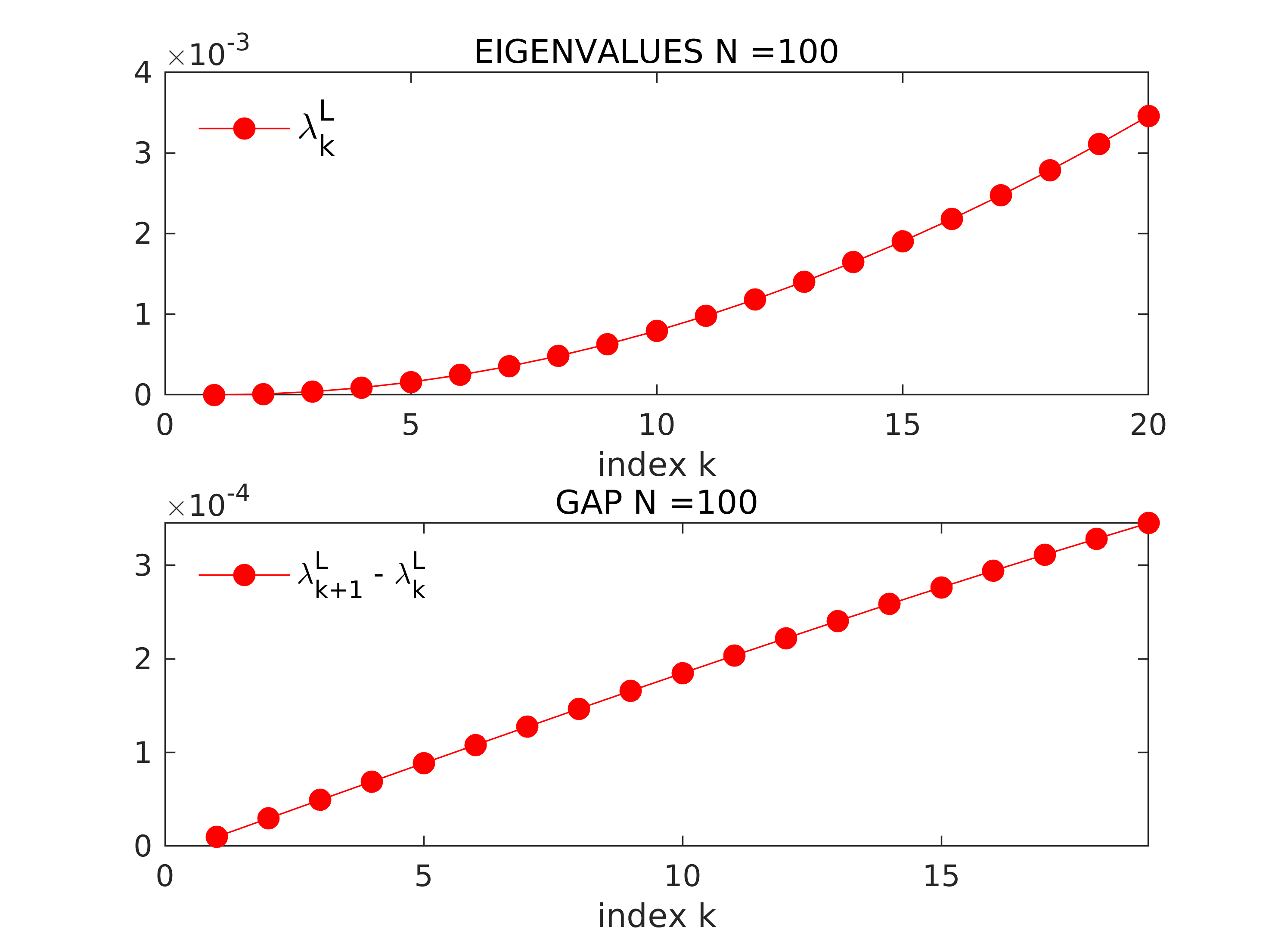
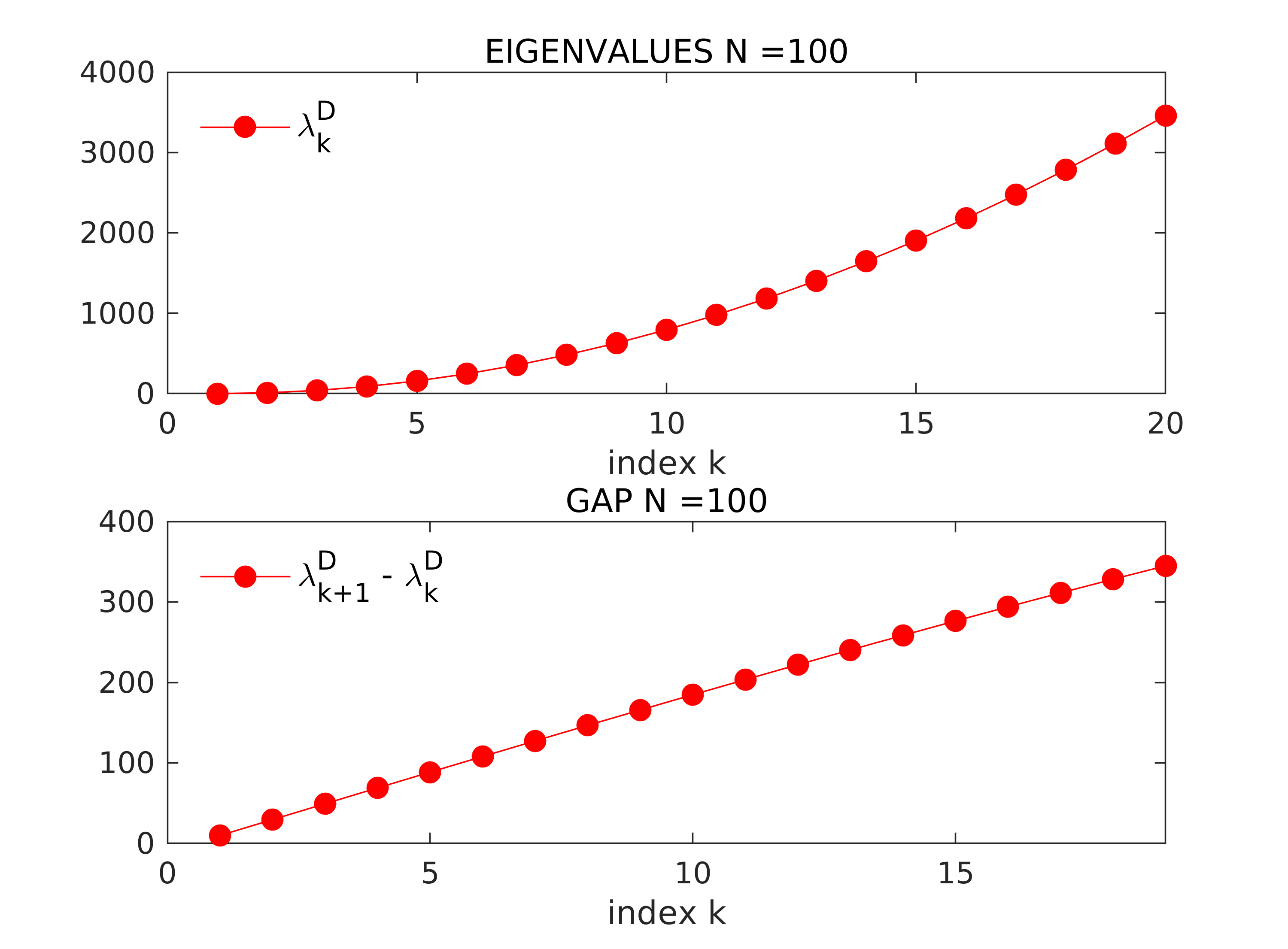
Figure 6. First twenty eigenvalues of (4.3) (top-left) and (4.5) (top-right) for $N=100$. The corresponding spectral gap is plotted at the bottom.

This gives a further explanation of the bad controllability properties of (4.2) (see Proposition 4.1).

For completeness, we have to mention that spectral accumulation phenomena similar to the ones observed for (4.2) arise in other classes of models, such as PDEs with memory terms ([8, 19, 55]), the structurally damped wave equation ([56]), or the Benjamin-Bona-Mahony equation ([61]).

4.2. The network dynamics of the 2d semi-discrete heat equation

A second example of model on a sparse graph to which our previous analysis applies is related the finite difference semi-discretization of the two dimensional heat equation on a square domain, for instance $[0,1]\times[0,1]$.

Let us consider the following interaction graph in Figure 7 and let

                                             $\color[rgb]{1,0,0}\bullet\color[rgb]{0,0,0}$$\color[rgb]{1,0,0}\bullet\color[rgb]{0,0,0}$$\color[rgb]{1,0,0}\bullet\color[rgb]{0,0,0}$$\color[rgb]{1,0,0}\bullet\color[rgb]{0,0,0}$$\color[rgb]{1,0,0}\bullet\color[rgb]{0,0,0}$$\color[rgb]{1,0,0}\bullet\color[rgb]{0,0,0}$$\color[rgb]{1,0,0}\bullet\color[rgb]{0,0,0}$$\color[rgb]{1,0,0}\bullet\color[rgb]{0,0,0}$$\color[rgb]{1,0,0}\bullet\color[rgb]{0,0,0}$$\color[rgb]{1,0,0}\bullet\color[rgb]{0,0,0}$$\color[rgb]{1,0,0}\bullet\color[rgb]{0,0,0}$$\color[rgb]{1,0,0}\bullet\color[rgb]{0,0,0}$$\color[rgb]{1,0,0}\bullet\color[rgb]{0,0,0}$$\color[rgb]{1,0,0}\bullet\color[rgb]{0,0,0}$$\color[rgb]{1,0,0}\bullet\color[rgb]{0,0,0}$$\color[rgb]{1,0,0}\bullet\color[rgb]{0,0,0}$$\color[rgb]{1,0,0}\bullet\color[rgb]{0,0,0}$$\color[rgb]{1,0,0}\bullet\color[rgb]{0,0,0}$$\color[rgb]{1,0,0}\bullet\color[rgb]{0,0,0}$$\color[rgb]{1,0,0}\bullet\color[rgb]{0,0,0}$$\color[rgb]{1,0,0}\bullet\color[rgb]{0,0,0}$$\color[rgb]{1,0,0}\bullet\color[rgb]{0,0,0}$$\color[rgb]{1,0,0}\bullet\color[rgb]{0,0,0}$$\color[rgb]{1,0,0}\bullet\color[rgb]{0,0,0}$$\color[rgb]{1,0,0}\bullet\color[rgb]{0,0,0}$$\color[rgb]{1,0,0}\bullet\color[rgb]{0,0,0}$$\color[rgb]{1,0,0}\bullet\color[rgb]{0,0,0}$$\color[rgb]{1,0,0}\bullet\color[rgb]{0,0,0}$$\color[rgb]{1,0,0}\bullet\color[rgb]{0,0,0}$$\color[rgb]{1,0,0}\bullet\color[rgb]{0,0,0}$$\color[rgb]{1,0,0}\bullet\color[rgb]{0,0,0}$$\color[rgb]{1,0,0}\bullet\color[rgb]{0,0,0}$$\color[rgb]{1,0,0}\bullet\color[rgb]{0,0,0}$$\color[rgb]{1,0,0}\bullet\color[rgb]{0,0,0}$$\color[rgb]{1,0,0}\bullet\color[rgb]{0,0,0}$$\color[rgb]{1,0,0}\bullet\color[rgb]{0,0,0}$$\color[rgb]{1,0,0}\bullet\color[rgb]{0,0,0}$$\color[rgb]{1,0,0}\bullet\color[rgb]{0,0,0}$$\color[rgb]{1,0,0}\bullet\color[rgb]{0,0,0}$$\color[rgb]{1,0,0}\bullet\color[rgb]{0,0,0}$$\color[rgb]{1,0,0}\bullet\color[rgb]{0,0,0}$$\color[rgb]{1,0,0}\bullet\color[rgb]{0,0,0}$$\color[rgb]{1,0,0}\bullet\color[rgb]{0,0,0}$$\color[rgb]{1,0,0}\bullet\color[rgb]{0,0,0}$$\color[rgb]{1,0,0}\bullet\color[rgb]{0,0,0}$$\color[rgb]{1,0,0}\bullet\color[rgb]{0,0,0}$$\color[rgb]{1,0,0}\bullet\color[rgb]{0,0,0}$$\color[rgb]{1,0,0}\bullet\color[rgb]{0,0,0}$$\color[rgb]{1,0,0}\bullet\color[rgb]{0,0,0}$$\color[rgb]{1,0,0}\bullet\color[rgb]{0,0,0}$$\color[rgb]{0,0,1}\square\color[rgb]{0,0,0}$$\color[rgb]{0,0,1}\square\color[rgb]{0,0,0}$$\color[rgb]{0,0,1}\square\color[rgb]{0,0,0}$$\color[rgb]{0,0,1}\square\color[rgb]{0,0,0}$$\color[rgb]{0,0,1}\square\color[rgb]{0,0,0}$$\small{\color[rgb]{0,0,1}\bullet\color[rgb]{0,0,0}}$$\small{\color[rgb]{0,0,1}\bullet\color[rgb]{0,0,0}}$$\small{\color[rgb]{0,0,1}\bullet\color[rgb]{0,0,0}}$$\small{\color[rgb]{0,0,1}\bullet\color[rgb]{0,0,0}}$$\small{\color[rgb]{0,0,1}\bullet\color[rgb]{0,0,0}}$$(1,1)$$(1,2)$$(1,N)$$(1,j-1)$$(1,j)$$(1,j+1)$$(i,j-1)$$(i,j)$$(i,j+1)$$(i-1,j)$$(i+1,j)$…………

Figure 7. Disposition on the $N^{2}$ agents of the model. Each agent $(i,j)$ interacts with the four agents connected to him. The control acts on the blue nodes in the box.

$$\dot{\textbf{x}}+L\textbf{x}=B\bf{u}$$ (4.14)

describe the control problem corresponding to the collective dynamics (1.1). In (4.14), we consider the$N^{2}\times N$ control matrix $B=[I,0,\ldots,0]^{T}$, where $I$ is the $N\times N$ identity, while the Laplacian matrix $L$ is given by

$$L=\left(\begin{matrix}P_{1}&-I&0&\ldots&0\\ -I&P_{2}&-I&\ldots&0\\ \vdots&&\ddots&&\vdots\\ 0&\ldots&-I&P_{2}&-I\\ 0&\ldots&\ldots&-I&P_{1}\end{matrix}\right)_{N^{2}\times N^{2}},$$ (4.15)

with $P_{1}$ and $P_{2}$ defined as

$$P_{1}=\left(\begin{matrix}2&-1&0&\ldots&0\\ -1&3&-1&\ldots&0\\ \vdots&&\ddots&&\vdots\\ 0&\ldots&-1&3&-1\\ 0&\ldots&\ldots&-1&2\end{matrix}\right)_{N\times N},\quad P_{2}=\left(\begin{matrix}3&-1&0&\ldots&0\\ -1&4&-1&\ldots&0\\ \vdots&&\ddots&&\vdots\\ 0&\ldots&-1&4&-1\\ 0&\ldots&\ldots&-1&3\end{matrix}\right)_{N\times N}.$$

As in the one-dimensional case, this is associated with the five-points finite difference semi-discretization of the two-dimensional heat equation with homogeneous Neumann boundary condition, which is given by

$$\dot{\textbf{x}}+Q\textbf{x}=B{\bf{u}},\quad Q=N^{2}L_{c}.$$ (4.16)

Hence, once again, the controllability properties of (4.14) can be analyzed in terms of the ones of (4.16).

It is classically known (see [20, 88, 89]) that in order to obtain the controllability of (4.16) the control region has to be “large enough”, for instance, a neighborhood of one side of the boundary (marked with blue diamonds in Figure 7).

When addressing the controllability problem for (4.14), other issues analogous to the one-dimensional case previously discussed arise. In particular, we find again that the control cost associated to (4.14) is $\exp(CN^{2}/T)$. Thus, the discussion in Section 4.1 applies again, and we can conclude that also in this case the controllability properties of (4.14) are badly behaved as $N\to+\infty$.

This gives a further account of the pathologies that may arise when considering a model on a sparse graph. Of course this example can be generalized to networks in any euclidean dimension. The same results hold if the control acts in the interior nodes within a fixed horizontal or vertical strip.

4.3. Consensus models on a dense graph

In Sections 4.1 and 4.2, we presented a couple of practical examples of consensus models (1.1) on sparse graphs, which have bad controllability properties because of the weakness of the interactions $a_{i,j}$.

We conclude our discussion presenting a couple of examples of consensus models on dense graphs. Recall that, in this case, the limit equation (1.2) will be a non-trivial one (that is, $W(s,s_{*})\neq 0$).

4.3.1. The model with a simple dense graph

Our first example is the following model with a periodic dense network (see Figure 8), similar to (3.8):

$$\dot{\textbf{x}}+L_{r}\textbf{x}=B{\bf{u}},\quad r\in[0,1/2].$$ (4.17)

In (4.17), the Laplacian matrix $L_{r}$ is given by

$$L_{r}=(l_{i,j})_{i,j=1}^{N},\quad l_{i,j}=\begin{cases}2,\quad&\text{if}\leavevmode\nobreak\ i=j,\\ -1/\ell,\quad&\text{if}\leavevmode\nobreak\ 0<|j-i|\leq\ell\textrm{ or }|j-i|>N-\ell,\\ 0,\quad&\text{otherwise},\end{cases}$$ (4.18)

with $\ell=[rN]$, where $[rN]$ denotes the closest integer to $rN$. Moreover, we consider a control $B$ as in (4.10).

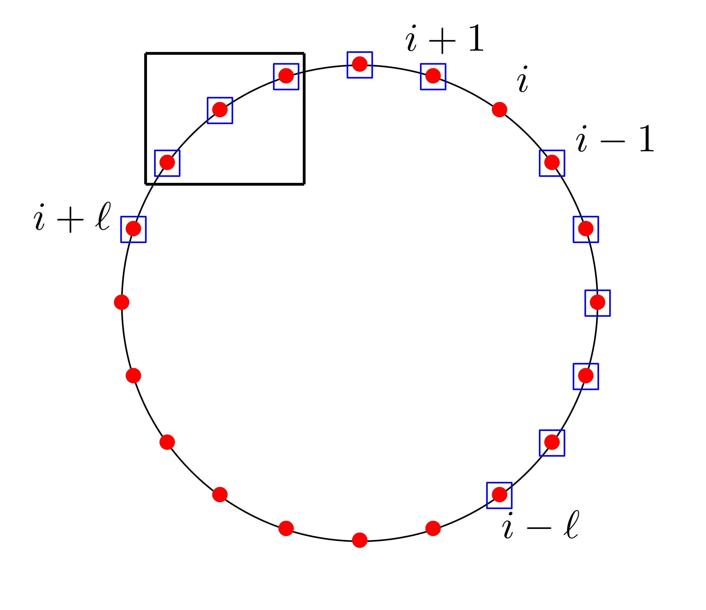
Figure 8. Disposition of the $N$ agents of the model. The agent $i$ interacts only with $j$, $j=i-\ell,\ldots,i+\ell$. The control acts on the agents in the black box.

In this model, each agent communicates with $2\ell=2[rN]$ other agents, and the number of agents with which communication is ensured increases with $N$. This is in contrast with the system (4.2), reminiscent from the finite difference discretization of the heat equation, in which each agent was only interacting with other two, one on the left and one on the right.

A relevant feature of this model is that the intensity of communication among the different agents is always the same, independent on their distance $|i-j|$, but decreases as $N$ increases to compensate the fact that effective interaction takes place with a increasing umber of agents. This is reflected also in the graph limit of (4.17) which, following [57], is given by the equation (see (3.11))

$$\partial_{t}x(\theta,t)=\frac{1}{2\pi r}\int_{\mathbb{S}^{1}}\chi_{[0,2\pi r]}(|\theta_{*}-\theta|)(x(\theta_{*},t)-x(\theta,t))\,d\theta_{*},\quad\theta\in\mathbb{S}^{1},\,t>0.$$

As we did in Section 4.1, in order to discuss controllability properties of (4.17) we analyze the spectrum of the Toeplitz matrix $L_{r}$, whose eigenvalues can be computed explicitly (see [78]):

$$\lambda_{k}^{r}=2-\frac{2}{\ell}\sum_{j=1}^{\ell}\cos\left(\frac{2k\pi j}{N}\right),\quad k=1,\ldots,N,$$

and are associated to plane-wave eigenvectors $\phi_{k}=\left(e^{i\frac{2k\pi j}{N}}\right)_{j=1}^{N}$, $k=1,\ldots,N$.

Notice that these eigenvalues may not be in ascending order, due to the presence of the sinusoidal function. Hence, to study the spectral gap analytically is not an easy task.

For this reason, in what follows we will only address an heuristic analysis of the spectral properties of (4.18), by showing the behavior of the eigenvalues and comparing them with the ones of (4.3).

We start by choosing the particular value $r=1/4$, which means that each agent is communicating with the fifty percent of the other agents in the network, and considering different values for $N$, namely $N=7,40$.

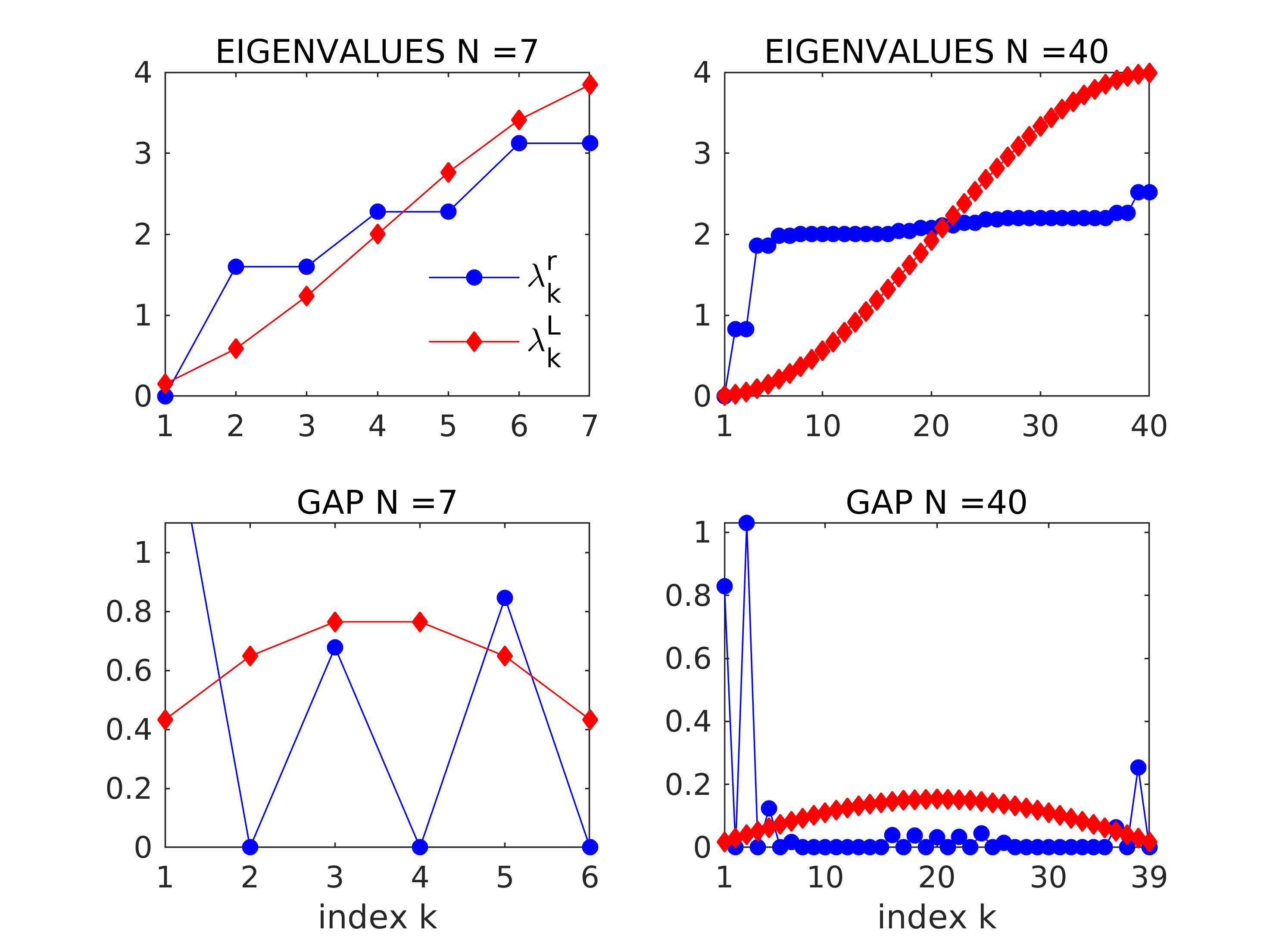
Figure 9. Eigenvalues (top) and spectral gap (bottom) of (4.18) (blue circles) and (4.3) (red diamonds). We consider $r=1/4$ and different values of $N=7,40$.

As we see in Figure 9, (4.17) has worst spectral properties than (4.2) from a control perspective. In particular, as $N$ increases the eigenvalues tends to accumulate more and more. Hence, the conditions (4.1) ensuring the controllability of (4.17) are once again not uniform and badly behaved in $N$.

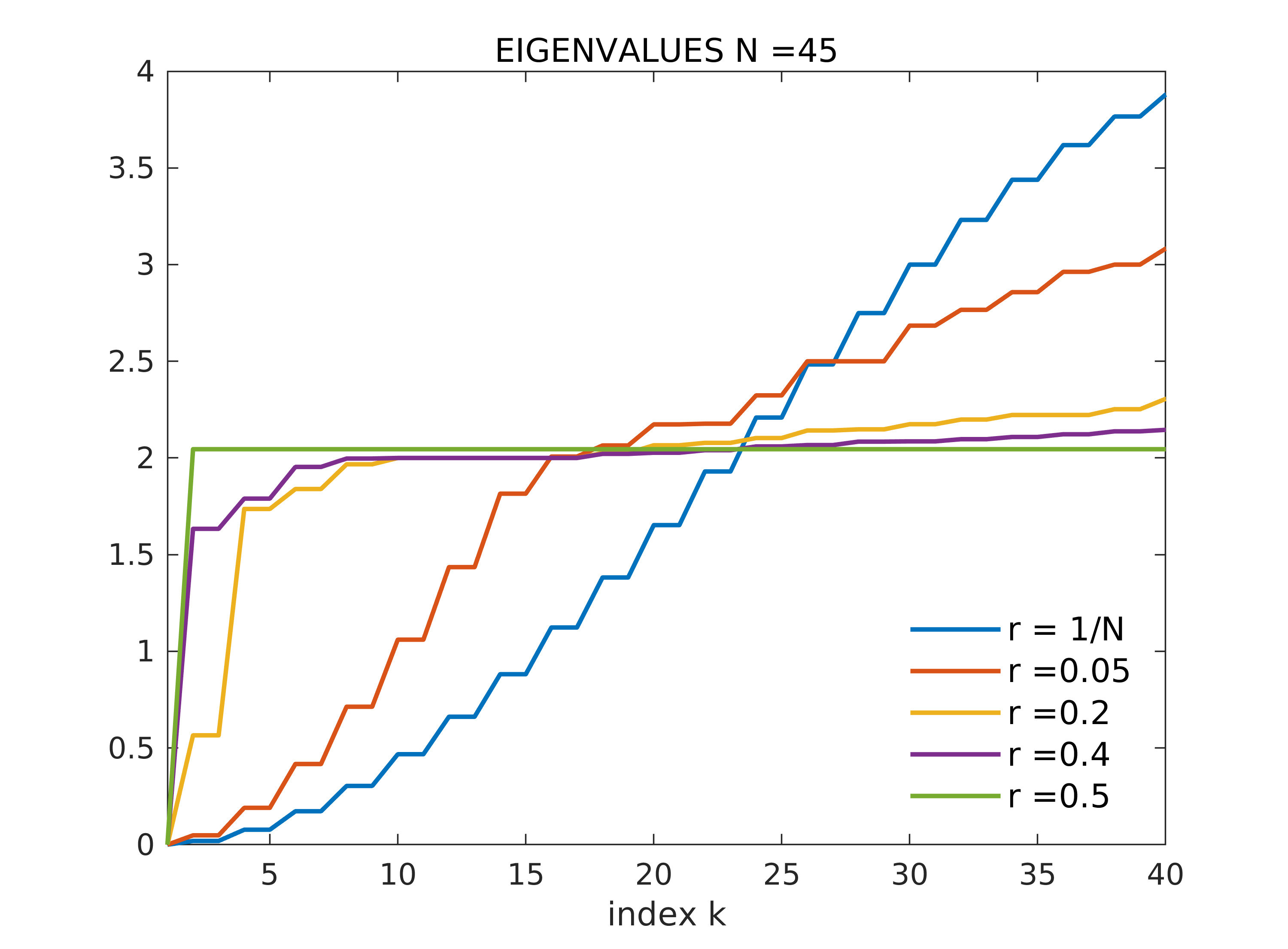
Figure 10. Distribution of the eigenvalues of (4.18) for fixed $N=45$ and different values of $r\in[0,1/2]$.

In Figure 10, instead, we are showing the evolution of the eigenvalues of (4.18) for a fixed value of $N$ (namely $N=45)$ and different values of $r$, for keeping track of their behavior in terms of the total percentage of interactions among the agents. We can clearly see that the accumulation of the spectrum increases for large values of $r$, that is, for very dense networks.

In conclusion, this example shows that having a dense network underneath the model (1.1) may not be enough to have uniform (with respect to $N$) controllability properties for the system, which are then transferred to the corresponding infinite-agent equation. In fact, the strength of the connections is also relevant. As a validation of that, we analyze in the next section a second example of consensus model on a dense graph associated to a fractional diffusion equation.

4.3.2. A fractional Laplacian network

As a final example of consensus model on a dense graph, let us consider the following equation

$$\dot{\textbf{x}}+L_{frac}\textbf{x}=B{\bf{u}},$$ (4.19)

where, for all $\alpha\in(0,1)$, the matrix $L_{frac}$ is defined as

$$L_{frac}=(a_{i,j})_{i,j=1}^{N},\quad a_{i,j}=\begin{cases}\displaystyle-\frac{c(\alpha)}{|i-j|^{1+2\alpha}},\quad&\text{if}\leavevmode\nobreak\ j\neq i,\\[10.0pt] \displaystyle\sum_{j\neq i}a_{i,j},\quad&\text{if}\leavevmode\nobreak\ i=j.\end{cases}$$ (4.20)

In (4.19), in contrast with (4.18), the communication rate among different agents is weighted as a function of the distance $|i-j|$. Hence, although the graphs underneath (4.19) and (4.17) are dense in both cases, in the former one the interactions are also weighted, and the ones among close agents have a higher impact on the dynamics.

Moreover, in this case, we consider a control strategy in which the matrix $B$ is given by (4.10).

According to (4.20), $L_{frac}$ describes a dense network inspired on the fractional Laplacian. Indeed, we can easily see that the matrix

$$D_{frac}:=N^{2\alpha}L_{frac}$$ (4.21)

is the finite difference discretization of the fractional Laplace operator ([22])

$$(-d_{x}^{2})^{\alpha}u(x):=c_{\alpha}P.V.\int_{\mathbb{R}}\frac{u(x)-u(y)}{|x-y|^{1+2\alpha}}dy,$$ (4.22)

and

$$\dot{\textbf{x}}+D_{frac}\textbf{x}=B{\bf{u}}$$ (4.23)

is the semi-discretized control problem associated to the following fractional heat equation

$$\partial_{t}u+(-d_{x}^{2})^{\alpha}u=0,\quad t\geq 0.$$ (4.24)

Notice that (4.24) corresponds the non-local diffusive model (1.2) with

$$W(x,y)=|x-y|^{-1-2\alpha},$$ (4.25)

In [7, 62, 79], the controllability of (4.24) has been studied both at the continuous and discrete level by means of spectral analysis techniques. In particular, it has been proved that controllability holds for any $T>0$ if and only $\alpha 1/2$, but that it cannot be achieved for $\alpha\leq 1/2$.

Hence, we can use this result, together with the presentation in Section 4.1, to discuss the controllability properties of (4.19).

Let us start by analyzing the spectral properties of (4.21) and (4.22). According to [47], in this case the eigenvalues behave as (see Figure 11)

$$\lambda_{k}^{D}\sim k^{2\alpha},\quad k\geq 1.$$

Figure 11. Evolution of the eigenvalues of (4.20) and (4.22) for $\alpha\leq 1/2$ (top) and $\alpha>1/2$ (bottom).

Hence, the spectral conditions (4.1) are satisfied uniformly in $N$ only for $\alpha>1/2$ (see Figure 12). In particular, for (4.21) we have that

$$\sum_{k=1}^{N}\left(\lambda_{k}^{D}\right)^{-1}\geq N, \textrm{ for }\alpha\leq 1/2$$

$$\sum_{k=1}^{N}\left(\lambda_{k}^{D}\right)^{-1}\leq C<+\infty, \textrm{ for }\alpha>1/2$$

and

$$\inf_{k=1,\ldots,N-1}\left(\lambda_{D}^{frac}-\lambda_{k}^{D}\right)=\begin{cases}\lambda_{N}^{D}-\lambda_{N-1}^{D}=\mathcal{O}(N^{2\alpha-1}),&\textrm{ for }\alpha<1/2\\[10.0pt] \lambda_{2}^{D}-\lambda_{1}^{D}=\mathcal{O}(1),&\textrm{ for }\alpha\geq 1/2.\end{cases}$$

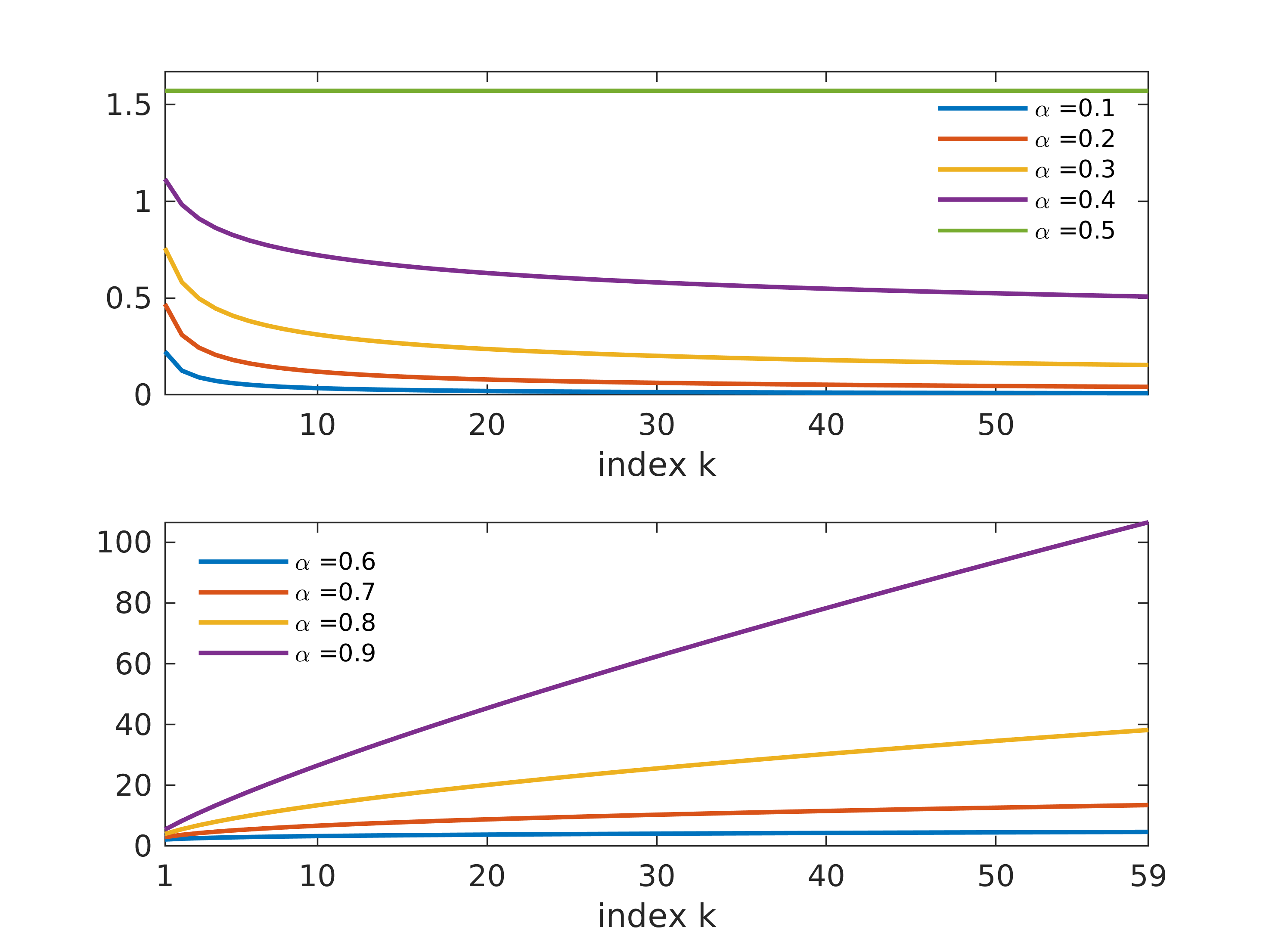
Figure 12. Evolution of the spectral gap of (4.20) and (4.22) for $\alpha\leq 1/2$ (top) and $\alpha>1/2$ (bottom).

Following [31, 32], this yields that, for $\alpha\leq 1/2$, the control cost for (4.23) is not bounded in $N$. In particular, for $\alpha<1/2$ it blows-up exponentially as $\exp(N^{1-2\alpha})$.

When considering the model (4.19), the situation is even worst and, even in the case $\alpha>1/2$, the controllability properties are not uniform in $N$ due to the scaling of the matrix (4.20)

First of all, from (4.21) we immediately have that the eigenvalues of (4.20) behave as

$$\lambda_{k}^{L}=N^{-2\alpha}\lambda_{k}^{D}\sim\left(\frac{k}{N}\right)^{2\alpha}$$

and, consequently, the spectral gap is very small even for $\alpha>1/2$ (see Figure 13).

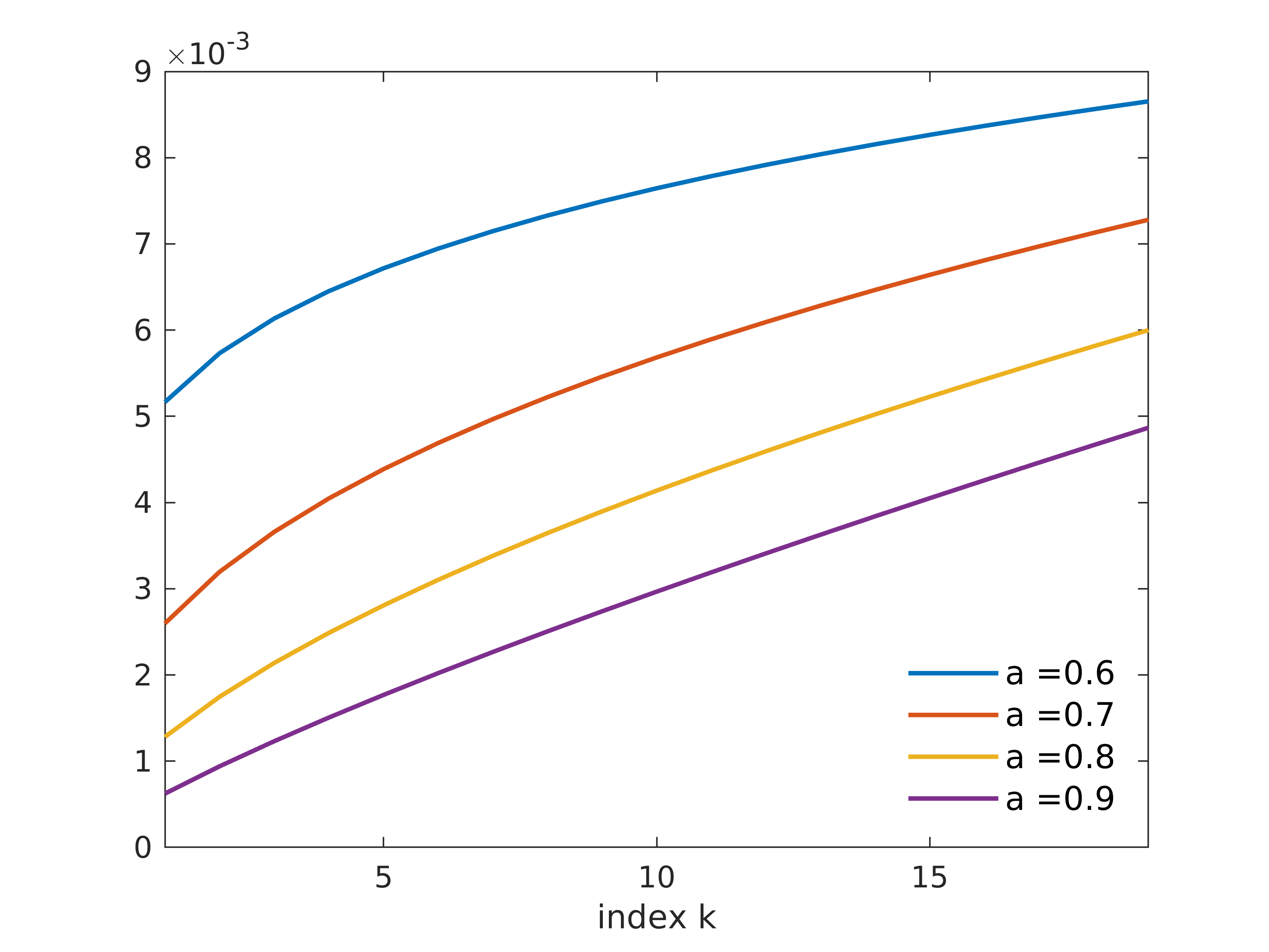
Figure 13. Evolution of the spectral gap of (4.20) for $\alpha>1/2$.

Moreover, systems (4.19) and (4.23) are equivalent up to time-scaling $t\mapsto N^{-2\alpha}t$:

$$\dot{\textbf{x}}+D_{frac}\textbf{x}=0,\;\;\;t\in[0,T/N^{2\alpha}].$$ (4.26)

Hence, following again the results in [90] we obtain that the cost of controlling (4.19) is of the order of $\exp(CN^{2\alpha}/T)$. This means that to control the system (4.19) with controls uniformly bounded on $N$ one needs not only $\alpha>1/2$, but also to take a control time of the order of $T\sim N^{2\alpha}$.

If instead the time horizon $T$ is fixed, independent of $N$, then the cost of controlling system (4.2) increases exponentially: $c(T)\sim\exp(CN^{2\alpha}/T)$.

These results are compatible with those in Section 4.1 for the network model inspired on the finite-difference approximation of the heat equation. In fact, when taking $\alpha=1$ in the discussion of the present section we recover the same estimates as in Section 4.1 on the cost of control.

5. Conclusions and open problems

In this article, we considered finite-dimensional collective behavior models and we discussed their infinite-agents limits. In addition, for linear networked systems, we also analyzed control properties.

First of all, we realized that the nature of the interactions among the individuals plays a crucial role in this limit process, and it determines the approach one should use when facing this issue. Namely, networked systems (2.1) require the employment of a graph limit ([57]), while for aligned ones (2.2) it is possible to rely on the classical mean-field theory ([64]).

These two limit approaches lead to substantially different kinds of equations, a diffusion and a transport one, respectively. In addition, a relevant difference between these two techniques is that the graph limit allows to track the evolution of each agent’s opinion individually, while mean-field only provides information only on their density. As a result, (1.4) describes a system in which individuals are indistinguishable. In addition, we showed that the diffusion equation (1.2) is subordinated to the transport one (1.3), and that (1.3) can be obtained by (1.2) through an averaging process.

Then we proposed a novel approach for analyzing the controllability to consensus of networked systems, which provides an alternative viewpoint with respect to the ones applied so far in this topic. In particular, we focused on the case where the control is acting only on a small amount of the agents.

Our idea is very simple: we suggest to relate these models to the finite-difference approximation of partial differential equations, and to rethink them under this new perspective.

We focused on some very specific example of models with linear interaction graphs and we showed how the network structure and the number of agents affect key properties such as the controllability time and cost. In particular, we showed that the cost for driving these systems to consensus is not uniform in $N$, and we described its divergent behavior as $N\to+\infty$.

Moreover, our analysis focused mainly on first-order models, although it can also be extended to second-order ones. In Section 3.6 we gave an account of this fact by heuristically describing the limit process and the corresponding PDEs. Notwithstanding, a rigorous convergence analysis still needs to be developed.

In addition, several interesting questions arise from our work:

1. In this paper, we never addressed the problem of finite-time controllability to consensus of nonlinear alignment models (1.1)-(2.2). Nevertheless, this is certainly an interesting issue and a natural continuation of our work. In particular, we shall be concerned with the analysis of the cost of controllability, in the same spirit of what we did in Section 4.

2. In Section 4.3.1, we briefly present an example of consensus model on a dense graph, in which the density of interactions strongly affects the controllability properties. A natural extension of our discussion would be to answer to the following question: given a network of $N$ agents, how can we determine how controllable the system is as a function of $N$? In particular, which is the minimum number of agents we have to control in order to reach consensus? These kinds of problems have been partially studied, for instance in [52], but a general theory is still unavailable.

3. It would be interesting to address a complete analysis of the controllability properties of second-order consensus models on networks which, according to our analysis, may be related to the semi-discretization of wave-like equations. In this context, we shall take into account that the finite difference semi-discretization may introduce unexpected behaviors of high-frequency solutions (see [76, 77, 88]) which may be inherited also from the collective behavior model.

4. Finally, a last interesting problem would be the analysis of the connection among first and second-order equations at all the levels (finite-dimensional models, graph and mean-field limit) that we described in this work. In the linear PDE setting this issue has already been largely discussed, for instance with the introduction of the transmutation concept based on the Kannai transform (see [28]). Hence, an analogous discussion applied to collective behavior models becomes an attractive topic which certainly deserves a deeper investigation.

References

- [1] Baccelli, F., Karpelevich, F., Kelbert, M. Y., Puhalskii, A., Rybko, A., and Suhov, Y. M. A mean-field limit for a class of queueing networks. J. Stat. Phys. 66, 3-4 (1992), 803–825.
- [2] Bardos, C., and Phung, K. D. Observation estimate for kinetic transport equations by diffusion approximation. C. R. Math. 355, 6 (2017), 640–664.
- [3] Bauso, D., Giarré, L., and Pesenti, R. Non-linear protocols for optimal distributed consensus in networks of dynamic agents. Syst. Control Lett. 55, 11 (2006), 918–928.
- [4] Bellomo, N., and Bellouquid, A. On multiscale models of pedestrian crowds from mesoscopic to macroscopic. Commun. Math. Sci 13, 7 (2015), 1649–1664.
- [5] Ben-Naim, E. Opinion dynamics: rise and fall of political parties. Europhys. Lett. 69, 5 (2005), 671.
- [6] Ben-Naim, E., Krapivsky, P., Vazquez, F., and Redner, S. Unity and discord in opinion dynamics. Phys. A 330, 1-2 (2003), 99–106.
- [7] Biccari, U., and Hernández-Santamaría, V. Controllability of a one-dimensional fractional heat equation: theoretical and numerical aspects. IMA J. Math. Control Inf. to appear (2019).
- [8] Biccari, U., and Micu, S. Null-controllability properties of the wave equation with a second order memory term. arXiv preprint arXiv:1807.03035 (2018).
- [9] Blondel, V. D., Hendrickx, J. M., Olshevsky, A., and Tsitsiklis, J. N. Convergence in multiagent coordination, consensus, and flocking. In Decision and Control, 2005 and 2005 European Control Conference. CDC-ECC’05. 44th IEEE Conference on (2005), IEEE, pp. 2996–3000.
- [10] Blondel, V. D., Hendrickx, J. M., and Tsitsiklis, J. N. On Krause’s multi-agent consensus model with state-dependent connectivity. IEEE Trans. Automat. Contr. 54, 11 (2009), 2586–2597.
- [11] Borgs, C., Chayes, J., Lovász, L., Sós, V. T., Szegedy, B., and Vesztergombi, K. Graph limits and parameter testing. In Proceedings of the thirty-eighth annual ACM symposium on Theory of computing (2006), ACM, pp. 261–270.
- [12] Braun, W., and Hepp, K. The Vlasov dynamics and its fluctuations in the 1/N limit of interacting classical particles. Comm. Math. Phys. 56, 2 (1977), 101–113.
- [13] Burini, D., and Chouhad, N. Hilbert method toward a multiscale analysis from kinetic to macroscopic models for active particles. Math. Models Methods Appl. Sci. 27, 07 (2017), 1327–1353.
- [14] Caponigro, M., Fornasier, M., Piccoli, B., and Trélat, E. Sparse stabilization and optimal control of the Cucker-Smale model. Math. Control Relat. Fields 3, 4 (2013), 447–466.
- [15] Caponigro, M., Piccoli, B., Rossi, F., and Trélat, E. Mean-field sparse Jurdjevic–Quinn control. Math. Models Methods Appl. Sci. 27, 07 (2017), 1223–1253.
- [16] Carrillo, J. A., Choi, Y.-P., and Hauray, M. The derivation of swarming models: mean-field limit and Wasserstein distances. In Collective dynamics from bacteria to crowds. Springer, 2014, pp. 1–46.
- [17] Carrillo, J. A., D’Orsogna, M. R., and Panferov, V. Double milling in self-propelled swarms from kinetic theory. Kinetic Relat. Models 2, 2 (2009), 363–378.
- [18] Carrillo, J. A., Fornasier, M., Toscani, G., and Vecil, F. Particle, kinetic, and hydrodynamic models of swarming. Mathematical modeling of collective behavior in socio-economic and life sciences (2010), 297–336.
- [19] Chaves-Silva, F. W., Zhang, X., and Zuazua, E. Controllability of evolution equations with memory. SIAM J. Control Optim. 55, 4 (2017), 2437–2459.
- [20] Chenais, D., and Zuazua, E. Controllability of an elliptic equation and its finite difference approximation by the shape of the domain. Numer. Math. 95, 1 (2003), 63–99.
- [21] Cucker, F., and Smale, S. Emergent behavior in flocks. IEEE Trans. Automat. Control 52 (2005).
- [22] Di Nezza, E., Palatucci, G., and Valdinoci, E. Hitchhiker’s guide to the fractional Sobolev spaces. Bull. Sci. Math. 136, 5 (2012), 521–573.
- [23] Diestel, R. Graph theory, vol. 173. Springer Heidelberg, 2005.
- [24] Dobrushin, R. L. Vlasov equations. Funct. Anal. Appl. 13, 2 (1979), 115–123.
- [25] Dorfler, F., and Bullo, F. Synchronization and transient stability in power networks and nonuniform Kuramoto oscillators. SIAM J. Control Optim. 50, 3 (2012), 1616–1642.
- [26] Duprez, M., Morancey, M., and Rossi, F. Approximate and exact controllability of the continuity equation with a localized vector field. arXiv preprint arXiv:1710.09287 (2017).
- [27] Duprez, M., Morancey, M., and Rossi, F. Minimal time problem for crowd models with a localized vector field.
- [28] Ervedoza, S., and Zuazua, E. Sharp observability estimates for heat equations. Arch. Rat. Mech. Anal. 202, 3 (2011), 975–1017.
- [29] Escobedo, R., Ibañez, A., and Zuazua, E. Optimal strategies for driving a mobile agent in a ”guidance by repulsion” model. Comm. Nonlin. Sci. Numer. Simul. 39 (2016), 58–72.
- [30] Fang, L., Antsaklis, P. J., and Tzimas, A. Asynchronous consensus protocols: preliminary results, simulations and open questions. In IEEE Conference on Decision and Control (2005), vol. 44, IEEE; 1998, p. 2194.
- [31] Fattorini, H. O., and Russell, D. L. Exact controllability theorems for linear parabolic equations in one space dimension. Arch. Rat. Mech. Anal. 43, 4 (1971), 272–292.
- [32] Fattorini, H. O., and Russell, D. L. Uniform bounds on biorthogonal functions for real exponentials with an application to the control theory of parabolic equations. Quart. Appl. Math. 32, 1 (1974), 45–69.
- [33] Golse, F. The mean-field limit for the dynamics of large particle systems. Journées équations aux dérivées partielles 9 (2003), 1–47.
- [34] Golse, F. The Boltzmann equation and its hydrodynamic limits. Evolutionary equations 2 (2005), 159–301.
- [35] Gupta, V., Hassibi, B., and Murray, R. M. On sensor fusion in the presence of packet-dropping communication channels. In Decision and Control, 2005 and 2005 European Control Conference. CDC-ECC’05. 44th IEEE Conference on (2005), IEEE, pp. 3547–3552.
- [36] Ha, S.-Y., Kim, H. K., and Ryoo, S. W. Emergence of phase-locked states for the Kuramoto model in a large coupling regime. Comm. Math. Sci. 14, 4 (2016), 1073–1091.
- [37] Ha, S.-Y., and Tadmor, E. From particle to kinetic and hydrodynamic descriptions of flocking. Kinetic Relat. Methods 1, 3 (2008), 415–435.
- [38] Hatano, Y., and Mesbahi, M. Agreement over random networks. IEEE Trans. Automat. Contr. 50, 11 (2005), 1867–1872.
- [39] Hilbert, D. Mathematical problems. Internat. Congress of Mathematicians, Paris. English transl.: Bull. Amer. Math. Soc. 37 (2000).
- [40] Hilbert, D. Begründung der kinetischen gastheorie. Math. Ann 72 (1912), 562–577.
- [41] Isaacson, E., and Keller, H. B. Analysis of numerical methods. Courier Corporation, 1994.
- [42] Jabin, P.-E., and Motsch, S. Clustering and asymptotic behavior in opinion formation. J. Differential Equations 257, 11 (2014), 4165–4187.
- [43] Jadbabaie, A., Motee, N., and Barahona, M. On the stability of the Kuramoto model of coupled nonlinear oscillators. In American Control Conference, 2004. Proceedings of the 2004 (2004), vol. 5, IEEE, pp. 4296–4301.
- [44] Kadanoff, L. P. More is the same; phase transitions and mean field theories. J. Stat. Phys. 137, 5-6 (2009), 777.
- [45] Krause, U. A discrete nonlinear and non-autonomous model of consensus formation. Comm. Diff. Equ. 2000 (2000), 227–236.
- [46] Kuramoto, Y., and Battogtokh, D. Coexistence of coherence and incoherence in nonlocally coupled phase oscillators. Nonlin. Phen. Complex Syst. 5, 4 (2002), 380–385.
- [47] Kwaśnicki, M. Eigenvalues of the fractional Laplace operator in the interval. J. Funct. Anal. 262, 5 (2012), 2379–2402.
- [48] Laing, C. R., and Chow, C. C. Stationary bumps in networks of spiking neurons. Neural Comput. 13, 7 (2001), 1473–1494.
- [49] Lasry, J.-M., and Lions, P.-L. Mean field games. Jpn J. Math. 2, 1 (2007), 229–260.
- [50] Le Boudec, J.-Y., McDonald, D., and Mundinger, J. A generic mean field convergence result for systems of interacting objects. In Quantitative Evaluation of Systems, 2007. QEST 2007. Fourth International Conference on the (2007), IEEE, pp. 3–18.
- [51] Lin, Z., Broucke, M., and Francis, B. Local control strategies for groups of mobile autonomous agents. IEEE Trans. Automat. Contr. 49, 4 (2004), 622–629.
- [52] Liu, Y.-Y., Slotine, J.-J., and Barabási, A.-L. Controllability of complex networks. Nature 473, 7346 (2011), 167.
- [53] Lovász, L. Large networks and graph limits, vol. 60. American Mathematical Soc., 2012.
- [54] Lovász, L., and Szegedy, B. Limits of dense graph sequences. J. Comb. Theory B 96, 6 (2006), 933–957.
- [55] Lü, Q., Zhang, X., and Zuazua, E. Null controllability for wave equations with memory. J. Math. Pures Appl. 108, 4 (2017), 500–531.
- [56] Martin, P., Rosier, L., and Rouchon, P. Null controllability of the structurally damped wave equation with moving control. SIAM J. Control Optim. 51, 1 (2013), 660–684.
- [57] Medvedev, G. S. The nonlinear heat equation on dense graphs and graph limits. SIAM J. Math. Anal. 46, 4 (2014), 2743–2766.
- [58] Medvedev, G. S. The nonlinear heat equation on w-random graphs. Arch. Rat. Mech. Anal. 212, 3 (2014), 781–803.
- [59] Mehyar, M., Spanos, D., Pongsajapan, J., Low, S. H., and Murray, R. M. Distributed averaging on asynchronous communication networks. In Decision and Control, 2005 and 2005 European Control Conference. CDC-ECC’05. 44th IEEE Conference on (2005), IEEE, pp. 7446–7451.
- [60] Mesbahi, M. On state-dependent dynamic graphs and their controllability properties. IEEE Trans. Automat. Contr. 50, 3 (2005), 387–392.
- [61] Micu, S. On the controllability of the linearized Benjamin-Bona-Mahony equation. SIAM J. Control Optim. 39, 6 (2001), 1677–1696.
- [62] Micu, S., and Zuazua, E. On the controllability of a fractional order parabolic equation. SIAM J. Control and Optimization 44, 6 (2006), 1950–1972.
- [63] Moshtagh, N., and Jadbabaie, A. Distributed geodesic control laws for flocking of nonholonomic agents. IEEE Trans. Automat. Contr. 52, 4 (2007), 681–686.
- [64] Motsch, S., and Tadmor, E. Heterophilious dynamics enhances consensus. SIAM Rev. 56, 4 (2014), 577–621.
- [65] Olfati-Saber, R. Flocking for multi-agent dynamic systems: Algorithms and theory. IEEE Trans. Automat. Contr. 51, 3 (2006), 401–420.
- [66] Olfati-Saber, R., Fax, J. A., and Murray, R. M. Consensus and cooperation in networked multi-agent systems. IEEE Proc. 95, 1 (2007), 215–233.
- [67] Olfati-Saber, R., and Murray, R. M. Distributed cooperative control of multiple vehicle formations using structural potential functions. In IFAC world congress (2002), vol. 15, Citeseer, pp. 242–248.
- [68] Olfati-Saber, R., and Shamma, J. S. Consensus filters for sensor networks and distributed sensor fusion. In Decision and Control, 2005 and 2005 European Control Conference. CDC-ECC’05. 44th IEEE Conference on (2005), IEEE, pp. 6698–6703.
- [69] Papachristodoulou, A., and Jadbabaie, A. Synchronization in oscillator networks: Switching topologies and non-homogeneous delays. In Decision and Control, 2005 and 2005 European Control Conference. CDC-ECC’05. 44th IEEE Conference on (2005), IEEE, pp. 5692–5697.
- [70] Preciado, V. M., and Verghese, G. C. Synchronization in generalized Erdös-Rényi networks of nonlinear oscillators. In Decision and Control, 2005 and 2005 European Control Conference. CDC-ECC’05. 44th IEEE Conference on (2005), IEEE, pp. 4628–4633.
- [71] Savkin, A. V. Coordinated collective motion of groups of autonomous mobile robots: Analysis of Vicsek’s model. IEEE Trans. Automat. Contr. 49, 6 (2004), 981–982.
- [72] Sepulchre, R., Paley, D., and Leonard, N. Collective motion and oscillator synchronization. In Cooperative control. Springer, 2005, pp. 189–205.
- [73] Spohn, H. Large scale dynamics of interacting particles. Springer Science & Business Media, 2012.
- [74] Sznitman, A.-S. Topics in propagation of chaos. In Ecole d’été de probabilités de Saint-Flour XIX—1989. Springer, 1991, pp. 165–251.
- [75] Tanaka, H.-A., Lichtenberg, A. J., and Oishi, S. Self-synchronization of coupled oscillators with hysteretic responses. Phys. D 100, 3-4 (1997), 279–300.
- [76] Trefethen, L. N. Group velocity in finite difference schemes. SIAM Rev. 24, 2 (1982), 113–136.
- [77] Vichnevetsky, R. Energy and group velocity in semi discretizations of hyperbolic equations. Math. Comput. Simul. 23, 4 (1981), 333–343.
- [78] Vichnevetsky, R., and Bowles, J. B. Fourier analysis of numerical approximations of hyperbolic equations, vol. 5. Siam, 1982.
- [79] Warma, M., and Zamorano, S. Null controllability from the exterior of a one-dimensional nonlocal heat equation. arXiv preprint arXiv:1811.10477 (2018).
- [80] Watanabe, S., and Strogatz, S. H. Constants of motion for superconducting Josephson arrays. Phys. D 74, 3-4 (1994), 197–253.
- [81] Weisbuch, G., Deffuant, G., Amblard, F., and Nadal, J.-P. Meet, discuss, and segregate! Complexity 7, 3 (2002), 55–63.
- [82] Weiss, P. L’hypothèse du champ moléculaire et la propriété ferromagnétique. J. Phys. Theor. Appl. 6, 1 (1907), 661–690.
- [83] Wongkaew, S., Caponigro, M., and Borzi, A. On the control through leadership of the Hegselmann–Krause opinion formation model. Math. Models Methods Appl. Sci. 25, 03 (2015), 565–585.
- [84] Xi, W., Tan, X., and Baras, J. S. A stochastic algorithm for self-organization of autonomous swarms. In Decision and Control, 2005 and 2005 European Control Conference. CDC-ECC’05. 44th IEEE Conference on (2005), IEEE, pp. 765–770.
- [85] Xi, X., and Abed, E. H. Formation control with virtual leaders and reduced communications. In Decision and Control, 2005 and 2005 European Control Conference. CDC-ECC’05. 44th IEEE Conference on (2005), IEEE, pp. 1854–1860.
- [86] Xia, H., Wang, H., and Xuan, Z. Opinion dynamics: A multidisciplinary review and perspective on future research. International J. Knowledge Syst. Sci. 2, 4 (2011), 72–91.
- [87] Xiao, L., and Boyd, S. Fast linear iterations for distributed averaging. Syst. Control Lett. 53, 1 (2004), 65–78.
- [88] Zuazua, E. Propagation, observation, and control of waves approximated by finite difference methods. Siam Rev. 47, 2 (2005), 197–243.
- [89] Zuazua, E. Control and numerical approximation of the wave and heat equations. In International Congress of Mathematicians, Madrid, Spain (2006), vol. 3, pp. 1389–1417.
- [90] Zuazua, E. Controllability and observability of partial differential equations: some results and open problems. In Handbook of differential equations: evolutionary equations, vol. 3. Elsevier, 2007, pp. 527–621.