Imaginary time density functional calculation of ground states
for second – row atoms using CWDVR approach

Abstract

We have developed the Coulomb wave function discrete variable representation (CWDVR) method to solve the imaginary time dependent Kohn – Sham equation on the many – electronic second row atoms. The imaginary time dependent Kohn – Sham equation is numerically solved using the CWDVR method. We have presented that the results of calculation for second row $Li$, $Be$, $B$, $C$, $N$, $O$ and $F$ atoms are in good agreement with other best available values using the Mathematica 7.0 programm.

I Introduction

Numerical approach of many – electron systems is extremely difficult computation. Density functional theory (DFT) is a computational quantum mechanical modeling method used to investigate many – electron systems, in particular atoms, molecules, and the condensed phases ref1 . It provides a powerful alternative technique to ab – initio wave function approach, since the electron density $\rho(\vec{r})$ possesses only three spatial dimensions no matter how large the system is. The DFT proves accurate and computationally much less expensive than usual ab – initio wave function methods, such as a Hartree Fock method. However, the exchange – correlation energy functional, which is a functional of the total electron density is not known exactly, and thus approximate exchange – correlation energy functional must be used. The DFT based upon the Hohenberg – Kohn (HK) energy functional ref2 focuses on the solution of exchange – correlation energy and it had been used in many calculations of ground state properties an atomic system. The Kohn – Sham equation is shown to be solved by the Coulomb wave function discrete variable representation method. Since the CWDVR method is able to treat the Coulomb singularity naturally, it is suitable for atomic systems ref3 . In our previous article, we calculated the ground state properties for noble gas atoms, such as $He$, $Ne$ and $Ar$ atoms using the Coulomb wave function discrete variable representation (CWDVR) method ref33 .

In this paper, we present the solution of the Kohn-Sham equation on the ground state problem for the many – electronic second row – atoms by the CWDVR method. This paper consists of methodology and results by the CWDVR method. We show that ground state energy values calculated by the present method are in good agreement with other precise theoretical calculations.

II CWDVR Method

The DVR method has its origin in the transformation method devised by Harris et al ref4 , where it was further developed by Dickinson and Certain ref5 . Light et al. ref6 first explicitly used the DVR method as a basis representation for quantum problems, where after different types of DVR methods have found wide applications in different fields of physical and chemical problems ref7 . The DVR method gives an idea, associated basis functions are localized about discrete values of the coordinate under consideration. The DVR simplifies the evaluation of Hamiltonian matrix elements. The matrix elements of kinetic energy can also be calculated very simply and analytically in most cases ref8 . In this section, we first give a brief introduction to the DVR constructed from orthogonal polynomials and Coulomb wave functions, which will be used to solve the Kohn – Sham equation for many – electron atomic systems.

The DVR approach basis functions can be constructed from any complete set of orthogonal polynomials, defined in the domain with the corresponding weight function ref8 . It is known that a Gaussian quadrature can also be constructed using nonclassical polynomials. The DVR derived from the Legendre polynomials has been shown by Machtoub and Zhang ref9 to provide very precise results for the metastable states of the exotic helium atom.

An appropriate quadrature rule for the Coulomb wave function was given by Dunseath et al ref10 with explicit expressions for the weights. The time dependent single particle Kohn – Sham equation has the form

$$i\frac{\partial\psi_{j}(\vec{r},t)}{\partial t}=(\widehat{H}_{0}+\upsilon_{eff})\psi_{j}(\vec{r},t),j=\overline{1,N}$$ (1)

Here, $\psi(\vec{r},t)$ the single particle Kohn – Sham orbit of $N$ electron atom, $\widehat{H}_{0}$ – atomic Hamiltonian, $\upsilon_{eff}$ is the time dependent effective potential, and charge density depends on the coordinates and time and is given by

$$\rho(\vec{r},t)=\sum^{N}_{j=1}|\psi_{j}(\vec{r},t)|^{2}$$ (2)

However, one can rewrite Eq.(1) in imaginary time $\tau$ and substitute $\tau=-it$, $t$ being the real time, to obtain a diffusion – type equations:

$$-\frac{\partial R_{j}(\vec{r},t)}{\partial t}=(-\frac{1}{2}\nabla^{2}+\upsilon_{eff})R_{j}(\vec{r},t)$$ (3)

The Kohn – Sham effective local potential contains both classical and quantum potentials and can be written as:

$$\upsilon_{eff}[\rho;\vec{r},t]=\frac{\delta E_{bb}}{\delta\rho}+\frac{\delta E_{ne}}{\delta\rho}+\frac{\delta E_{xc}}{\delta\rho}+\frac{\delta E_{ext}}{\delta\rho}$$ (4)

Here the first term is inter – electronic Coulomb repulsion, the second is the electron – nuclear attraction term, the third is exchange – correlation term, and last term comes from interaction with the external field (in the present case, this interaction is zero). A simple local energy functional form has been applied for the atoms, and the exchange part can be found to be ref11 ,

$$\frac{\delta E_{x}}{\delta\rho}=\frac{\delta E^{LDA}_{x}}{\delta\rho}-\beta\bigg{[}\frac{\frac{4}{3}\rho^{1/3}+\frac{2}{3}\frac{r^{2}\rho}{\alpha_{x}}}{(1+\frac{r^{2}\rho^{2/3}}{\alpha_{x}})^{2}}\bigg{]}$$ (5)

$$\frac{\delta E^{LDA}_{x}}{\delta\rho}=-\frac{4}{3}C_{x}\rho^{1/3}$$ (6)

The simple local parameterized Wigner – type correlation energy functional ref12 used for ground states:

$$E_{c}=-\int\frac{\rho}{a+b\cdot\rho^{-1/3}}d\vec{r}$$ (7)

$$\frac{\delta E_{c}}{\delta\rho}=-\frac{a+c\cdot\rho^{-1/3}}{(a+b\cdot\rho^{-1/3})^{2}}$$ (8)

where $a=9.81$, $b=21.437$, $c=28.582667$ are respectively. The solution of Eq.(1) is used split time method, for split time $\Delta t$. It can be written

$$R(\vec{r},t+\Delta t)\cong e^{-\Delta t\hat{H}_{0}/2}e^{-\hat{V}\Delta t}e^{-\Delta t\hat{H}_{0}/2}R(\vec{r},t)$$ (9)

One of the main features of the DVR is that a function $R(\vec{r},t)$ can be approximated by interpolation through the given grid points:

$$R(r)\cong\sum^{N}_{j=0}R(r_{j})\cdot g_{j}(r)$$ (10)

Here: $R(r_{j})$ is the interpolation function, $g_{j}(r)$ is the cardinal function.

The Coulomb wave function is defined by radial grid points. Interpolation function is obtained by using the radial function that is derived from the cardinal functions. By noting that $F(r)$ is the Coulomb function, $F^{\prime}(r)$ is the first derivative from F(r) at the position $r_{j}$, $\psi_{j}$ is found to be $\psi_{j}=\frac{R(r)}{F^{\prime}(r)}$. The propagation in the energy space (step first in equation) can now be achieved through

$$e^{-\hat{H}_{0}\Delta t/2}R(r)=\sum^{N}_{j=0}e^{-\hat{H}_{0}\Delta t/2}R(r_{j})g_{j}(r)$$ (11)

The cardinal functions $g_{j}(r)$ in (Eq.10) are given by the following expression

$$g_{j}(r)=\frac{1}{F^{\prime}(r_{j})}\frac{F(r)}{r-r_{j}}$$ (12)

where the points $r_{j}$ ($j=1,2,...,N$) are the zeros of the Coulomb wave function $F(r)$ and $F^{\prime}(r_{j})$ stands for its first derivative at $r_{j}$ and $g_{j}(r)$ satisfies the cardinality condition

$$g_{j}(r_{i})=\delta_{ji}.$$ (13)

Since the Coulomb wave functions was expressed in quadrature rule with expressions for the weight $\omega_{j}$, then DVR basis function $F_{j}(r)$ satisfies the eigenvalue for the radial Kohn – Sham type equation:

$$\hat{H}(r)\psi(r)=E\psi(r)$$ (14)

and

$$\hat{H}(r)=-\frac{d^{2}}{2d^{2}}+V(r).$$ (15)

The DVR greatly simplifies the evaluation of Hamiltonian matrix elements. The potential matrix elements involve merely the evaluation of the interaction potential at the DVR grid points, where no integration is needed. The DVR basis function $f_{j}(r)$ is constructed from the cardinal function $g_{j}(r)$ as follows

$$f_{j}(r)=\frac{1}{\sqrt{\omega_{j}}}g_{j}(r),$$ (16)

here the weight $\omega_{j}$ is given in ref10 :

$$\omega_{j}\approx\frac{\pi}{a^{2}_{j}}.$$ (17)

$$a_{j}=F^{\prime}(r_{j}).$$ (18)

The second derivative of the cardinal function $g^{{}^{\prime\prime}}_{j}(r_{j})$ is given by

$$g^{{}^{\prime\prime}}_{j}(r_{j})=\delta_{jk}\frac{c_{k}}{3a_{k}}-(1-\delta_{jk})\frac{a_{k}}{a_{j}}\frac{2}{(r_{k}-r_{j})^{2}},$$ (19)

where $a_{k}$ is given by Eq.(18) and $c_{k}$. Here kinetic energy matrix elements $D_{ij}$ calculated using:

$$c_{k}=-a_{k}(2E+2Z/r),$$ (20)

$$D_{ji}=-\delta_{ij}\frac{c_{i}}{6a_{i}}+(1-\delta_{ji})\frac{1}{(r_{i}-r_{j})^{2}},$$ (21)

In the Eq.(15), to expand $R(r_{j})$ in the eigenvectors of the Hamiltonian $\hat{H}_{0}$, we first solve the eigenvalue problem for $\hat{H}_{0}$ after discretization of coordinate, the differential equation for this problem can be written as:

$$\sum^{N}_{j=1}\bigg{[}-\frac{1}{2}D_{ji}+V(r_{j})\delta_{ji}\bigg{]}\phi_{kj}=\varepsilon_{k}\phi_{kj}$$ (22)

Here $D_{ji}$ denotes the symmetrized second derivative of the cardinal function that is given as,

$$(D_{2})_{ji}=\frac{1}{3}(E+\frac{Z}{r}),\qquad j=i$$ (23)

$$(D_{2})_{ji}=\frac{1}{(r_{i}-r_{j})^{2}},\qquad j\neq i.$$ (24)

The Eq.(2) is then numerically solved to achieve a self – consistent set of orbitals, using the DVR method. These orbitals are used to construct various Slater determinants arising out of that particular electronic configuration and its energies computed in the usual manner. A key step in the time propagation of Eq.(9) is to construct the evolution operator $e^{-\hat{H}^{0}_{l}\Delta t/2}\cong S(l)$ through an accurate and efficient representation of $\hat{H}^{0}_{l}$. Here we extend the DVR method to achieve optimal grid discretization and an accurate solution of the eigenvalue problem of $\hat{H}^{0}_{l}$.

In the present work, we are particularly interested in the exploration of the improvement of the Kohn – Sham type equation in electron structure calculation. Thus we choose the Slater wave function as our initial state at $t=0$. Note that, the differential equation for time propagation is normalized at the each time step. Here the 152 grid points are used for the DVR discretization of the radial coordinates and $\Delta t=0.001au.$, with 500 iteration is used in the time propagation to achieve convergence.

III Calculation and Results

In this section we present results from nonrelativistic electronic structure calculation of the ground states of $Li$, $Be$, $B$, $C$, $N$, $O$ and $F$ atoms. Here, parameters of the Coulomb wave function such as wave number and effective charges are chosen to be $k=\sqrt{2E}=3$ and $Z1=400$ . Table 1 summarizes the main results for mentioned atoms. The first row shows the present results. The results from the Amlan K Roy ref13 for energies for the ground states for $Li$, $Be$, $B$, $C$, $N$, $O$ and $F$ atoms are shown below the present results. The corresponding HF values from the literature are listed for comparison. For all atoms except F (mismatch 3.1%), we found the present results of the total electronic energies are considerably match the HF values and are significantly better than the results from Amlan K Roy ref13 .

Table 1: Calculated ground – state properties of $Li$, $Be$, $B$, $C$, $N$, $O$ and $F$ atoms (by the unit of $au.$) along with literature data for comparison.

		$Li$	$Be$	$B$	$C$	$N$	$O$	$F$
$-E$	Present work	7.3197	14.582	24.779	37.9484	55.625	75.795	102.897
	Roy [13]	7.221	14.22 1	23.964	36.953	53.407	73.451	99.734
	HF [2]	7.4332	14.573	24.529	37.688	54.400	74.809	99.400
$-Z/r$	Present work	17.054	33.447	56.728	88.447	128.915	179.317	240.433
	Roy [13]	17.115	34.072	58.143	88.649	127.326	176.324	-
$-E_{x}$	Present work	1.752	2.656	3.732	5.0416	6.527	8.223	10.147
	Roy [13]	1.574	2.404	3.478	4.640	5.987	7.490	10.000
	HF [2]	1.781	2.667	3.744	5.045	6.596	8.174	10.020
$-E_{c}$	Present work	0.0659	0.093	0.1252	0.1637	0.2058	0.2524	0.303
	Roy [13]	0.154	0.322	0.302	0.368	0.434	0.543	-
	HF [2]	0.0435	0.094	0.111	0.1560	0.1890	0.2414	0324
$T$	Present work	7.301	14.172	23.888	37.301	53.536	74.825	98.193
	Roy [13]	7.382	14.844	25.300	37.924	53.664	73.444	98.372
	HF [2]	7.433	14.573	24.529	37.688	54.401	74.810	99.410

It is satisfying that the CWDVR approach can be used to perform high precision calculation of the Kohn – Sham type equation with the use of only a few of grid points.

Analyses of the results for exchange and correlation energies are given in the same table separately. The results from exchange energies ($E_{x}$) calculations of the present calculations show a good agreement with the HF results ref2 . For the $Li$, $Be$, $B$, $C$ and $F$ atoms, the calculated exchange energy is nearly exact, while for $N$, $O$ and $F$ there is an underestimation about $1.1\%$. This indicates that the simple local exchange functional in Eq.(5) is well accurate, compare to those of Amlan J Roy ref13 .

The ”exact” correlation energies are considered for the$Li$, $Be$, $B$, $C$, $N$, $O$ and $F$ atoms in the Table 1 due to the comparison with other results. The Wigner – type correlation energy functional is likely seem to be sufficiently enough for the systems considered. For the $Be$ atom, it is nearly exact, otherwise underestimated by about $5.1-12.5\%$; the $Li$ atom is being the worst case. Compared with other generalized – gradient approximations (GGA), Perdew’s GGA ref14 correlation energy functional gives better results for $Be$, $B$ and $C$ but worse results for $Li$, $N$, $O$ and $F$. We note that the primary purpose of this work is to explore the feasibility of extending the CWDVR to the solution of the Kohn – Sham type differential equation with imaginary time propagation. The LDA – type $E_{xc}$ energy functionals can be easily adopted in the present CWDVR approach. Table 1 shows that the Viral theorem is nearly satisfied for $Li$, $Be$, $B$ and $C$ atoms. The calculated kinetic energy term for the $Li$ atom is reasonably exact to HF, while for rest atoms there is an underestimation by $2.1-4.3\%$. In Figures 1 and 2, the radial density plots for lithium, boroncarbon and nitrogen are presented, where HF plot is not shown. In Figure 3, we report the radial density plots for beryllium. The inset (a) reports the result from present calculation; the inset (b) shows the HF plot for comparison. Here, the radial density plot shape from our calculation is in good agreement with the HF plot.

IV Conclusions

In conclusion, we present that the nonrelativistic ground state properties of $Li$, $Be$, $B$, $C$, $N$, $O$ and $F$ atoms can be calculated by means of time – dependent Kohn – Sham equations and an imaginary time evolution methods. The CWDVR approach shown to be an efficient and precise solution of ground – state energies of atoms. The calculated electronic energies are in good agreement with the HF values and are significantly better than the results in the other literatures. The approach is likely opens a road to solution of ionization and excitation states of many electron atoms.

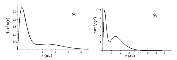
Figure 1: Radial density plot of (a) $Li$ and (b) $B$ (by unit of $au.$).

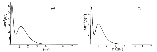
Figure 2: Radial density plot of (a) $C$ and (b) $N$ (by unit of $au.$).

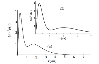
Figure 3: Radial density plot of $Be$ (by unit of $au.$).

- (1) P. Hohenberg and W. Kohn, Phys. Rev. 136, B864 (1964).
- (2) R. G. Parr and W. Yang, Density – Functional Theory of Atoms and Molecules, Oxford Univ. Press, New York, (1989).
- (3) Liang – You Peng and Anthony F. Starace, J. Chem. Physics 125, 154311 (2006).
- (4) D. Naranchimeg, L. Khenmedekh, G. Munkhsaikhan and N. Tsogbadrakh, Mongolian Journal of Physics, 3, 55 (2017); arXiv:1810.01085 (2018).
- (5) D. O. Harris, G. G. Engerholm, and W. D. Gwinn, J. Chem. Phys. 43,1515 (1965).
- (6) A. S. Dickinson and P. R. Certain, J. Chem. Phys. 49, 4209 (1968).
- (7) J. V. Lill, G. A. Parker, and J. C. Light, Chem. Phys. Lett. 89, 483 (1982); R. W. Heather and J. C. Light, J. Chem. Phys. 79, 147 (1983).
- (8) C. Light, I. P. Hamilton, and J. V. Lill, J. Chem. Phys. 82, 1400 (1985).
- (9) D. Baye and P. H. Heenen, J. Phys. A 19, 2041 (1986); V. Szalay, J. Chem. Phys. 99, 1978 (1993).
- (10) G. Machtoub and C. Zhang, Int. J. Theor. Phys. 41, 293 (2002).
- (11) K. M. Dunseath, J. M. Launay, M. Terao-Dunseath, and L. Mouret, J.Phys. B35, 3539 (2002).
- (12) B. M. Deb and P. K. Chattaraj, Phys. Rev. A 39, 1696 (1989).
- (13) Amlan K Roy and Shih – I Chu, J. Phys. B: At. Mol. Opt. Phys.35,2075 (2002).
- (14) Amlan K Roy, J. Math Chem. 49, 1687 (2011).
- (15) J. P. Perdew, Phys.Rev.B 33, 8822 (1986).