ABSTRACT

In the recent years, the field of fast radio bursts (FRBs) is thriving and growing rapidly. It is of interest to study cosmology by using FRBs with known redshifts. In the present work, we try to test the possible cosmic anisotropy with the simulated FRBs. In particular, we only consider the possible dipole in FRBs, rather than the cosmic anisotropy in general, while the analysis is only concerned with finding the rough number of necessary data points to distinguish a dipole from a monopole structure through simulations. Noting that there is no a large sample of actual data of FRBs with known redshifts by now, simulations are necessary to this end. We find that at least 2800, 190, 100 FRBs are competent to find the cosmic dipole with amplitude 0.01, 0.03, 0.05, respectively. Unfortunately, even 10000 FRBs are not competent to find the tiny cosmic dipole with amplitude of ${\cal O}(10^{-3})$. On the other hand, at least 20 FRBs with known redshifts are competent to find the cosmic dipole with amplitude 0.1. We expect that such a big cosmic dipole could be ruled out by using only a few tens of FRBs with known redshifts in the near future.

Cosmic Anisotropy and Fast Radio Bursts

I Introduction

In the past few years, the newly discovered fast radio bursts (FRBs) have become a promising field in astronomy and cosmology, which is currently thriving and growing rapidly Keane:2018jqo ; Lorimer:2018rwi ; Pen:2018ilo ; Kulkarni:2018ola ; Burke-Spolaor:2018xoa ; Macquart:2018fhn ; NAFRBs . In fact, since its first discovery Lorimer:2007qn , more and more evidences suggest that FRBs are at cosmological distances (see e.g. Thornton:2013iua ; Champion:2015pmj ; Spitler:2016dmz ; Tendulkar:2017vuq ; Marcote:2017wan ; Chatterjee:2017dqg ; Keane:2016yyk ; Shannon:2018ASKAP ; Amiri:2019qbv ; Amiri:2019bjk ; Petroff:2016tcr ). So, it is reasonable to consider the cosmological application of FRBs.

One of the key measured quantities of FRBs is the so-called dispersion measure (DM). According to the textbook Rybicki:1979 (see also e.g. Deng:2013aga ; Yang:2016zbm ; Ioka:2003fr ; Inoue:2003ga ), an electromagnetic signal of frequency $\nu$ propagates through an ionized medium (plasma) with a velocity $\displaystyle v=c\,(1-\nu_{p\;}^{2}/\nu^{2})^{1/2}$, less than the speed of light in vacuum $c$, where $\displaystyle\nu_{p}=(n_{e}\,e^{2}/\pi m_{e})^{1/2}\simeq 8.98\times 10^{3}\,n_{e}^{1/2}\;{\rm Hz}$ is the plasma frequency, $n_{e}$ is the number density of free electrons in the medium (given in units of $\rm cm^{-3}$), $m_{e}$ and $e$ are the mass and charge of electron, respectively. Therefore, an electromagnetic signal with frequency $\nu\gg\nu_{p}$ is delayed relative to a signal in vacuum by a time Rybicki:1979 ; Deng:2013aga ; Yang:2016zbm ; Ioka:2003fr ; Inoue:2003ga

$$t_{p}\simeq\int\frac{\nu_{p}^{2}}{2\nu^{2}}\frac{dl}{c}=\frac{e^{2}}{2\pi m_{e\,}c}\frac{1}{\nu^{2}}\int n_{e}\,dl\equiv\frac{e^{2}}{2\pi m_{e\,}c}\frac{\rm DM}{\nu^{2}}\simeq 4.2\,{\rm s}\,\left(\frac{\nu}{\rm GHz}\right)^{-2}\frac{\rm DM}{10^{3}\;{\rm pc\hskip 2.40005ptcm^{-3}}}\,,$$ (1)

where the dispersion measure ${\rm DM}=\int n_{e}\,dl$ means actually the column density of the free electrons. In practice, it is convenient to measure the time delay between two frequencies. For a plasma at redshift $z$, the rest frame (infinitesimal) time delay between two rest frame frequencies is given by

$$dt_{z}=\frac{e^{2}}{2\pi m_{e\,}c}\,\bigg{(}\frac{1}{\nu_{1,\,z}^{2}}-\frac{1}{\nu_{2,\,z}^{2}}\bigg{)}\,n_{e,\,z}\,dl\,.$$ (2)

In the observer frame, the observed time delay and the observed frequency are both redshifted, namely $dt=dt_{z}\,(1+z)$, and $\nu=\nu_{z}/(1+z)$. So, the the observed time delay is given by Deng:2013aga ; Yang:2016zbm ; Ioka:2003fr ; Inoue:2003ga

$$\Delta t=\int dt=\frac{e^{2}}{2\pi m_{e\,}c}\left(\frac{1}{\nu_{1}^{2}}-\frac{1}{\nu_{2}^{2}}\right)\int\frac{n_{e,\,z}}{1+z}\,dl\equiv\frac{e^{2}}{2\pi m_{e\,}c}\left(\frac{1}{\nu_{1}^{2}}-\frac{1}{\nu_{2}^{2}}\right){\rm DM}\,,$$ (3)

and the observed dispersion measure reads Deng:2013aga ; Yang:2016zbm ; Ioka:2003fr ; Inoue:2003ga

$${\rm DM}=\int\frac{n_{e,\,z}}{1+z}\,dl\,.$$ (4)

Using Eq. (3), one can observationally obtain DM by measuring $\Delta t$ between two frequencies $\nu_{1}$ and $\nu_{2}$. On the other hand, since the distance $dl$ along the path in Eq. (4) records the expansion history of the universe (see below in details), the observed DM can be used to study cosmology. It is worth noting that DM is traditionally used to observe pulsars in or nearby our Galaxy (Milky Way) and other objects, but now is also extended to FRBs since the first day that FRB was discovered.

For typical FRBs, the observed DM is ${\cal O}(10^{2})$ or ${\cal O}(10^{3})$ $\rm pc\hskip 2.40005ptcm^{-3}$ with negligible uncertainties of ${\cal O}(10^{-1})$ or ${\cal O}(10^{-2})$ $\rm pc\hskip 2.40005ptcm^{-3}$ Petroff:2016tcr , and $\nu\sim{\rm GHz}$, $\Delta t\sim{\rm ms}$. Most of the published FRBs are at high Galactic latitude $|b|>10^{\circ}$ Petroff:2016tcr , which is helpful to minimize the contribution of our Galaxy (Milky Way) to the electron column density, DM. As of 1 January 2020, 107 FRBs have been found Petroff:2016tcr mainly by the telescopes Parkes, UTMOST, ASKAP and CHIME. In particular, the number of FRBs increased rapidly after the (pre-)commissions of ASKAP and CHIME in 2018. In fact, the lower-limit estimates for the number of the FRB events occurring are a few thousand each day Keane:2018jqo ; Bhandari:2017qrj . Even conservatively, the FRB event rate floor derived from the pre-commissioning of CHIME is $3\times 10^{2}$ events per day Amiri:2019qbv . Thus, the observed FRBs will be numerous in the coming years.

As a very crude rule of thumb, the redshift $z\sim{\rm DM}/(1000\;\rm pc\hskip 2.40005ptcm^{-3})$ Lorimer:2018rwi . For all the 107 observed FRBs to date, their DMs are in the range $100\sim 2600\;\rm pc\hskip 2.40005ptcm^{-3}$ approximately Petroff:2016tcr , and hence one can infer redshifts in the range $0.1\lesssim z\lesssim 2.6$ crudely. In fact, the redshift of FRB 121102 Spitler:2016dmz ; Tendulkar:2017vuq ; Marcote:2017wan ; Chatterjee:2017dqg has been directly identified ($z=0.19273$ Tendulkar:2017vuq ), which is the only repeating FRB source before CHIME. Recently, the other 9 repeating FRB sources have been found by CHIME Amiri:2019bjk ; Andersen:2019yex , and it is reasonable to expect more repeating FRB sources in the future. As mentioned in e.g. Yang:2016zbm , there exist three possibilities to identify FRB redshifts in the future, namely (i) pin down the precise location and then the possible host galaxy of FRB (especially repeating FRB) by using VLBI observations Marcote:2019sjf . (ii) catch the afterglow of FRB by performing multi-wavelength follow-up observations soon after the FRB trigger Yi:2014jka . (iii) detect the FRB counterparts in other wavelengths (for example, gamma-ray bursts (GRBs)). Since the field of FRBs is growing rapidly, similar to the history of GRBs Kulkarni:2018ola , numerous FRBs with identified redshifts might be available in the coming years.

It is worth noting that the up-to-date online catalogue of the observed FRBs can be found in Petroff:2016tcr , which summarizes almost all observational aspects concerning the published FRBs. On the other hand, in the literature, a lot of theoretical models have been proposed for FRBs, and the number of FRB theories is still increasing. Since in the present work we are mainly interested in the observational aspects, we just refer to Platts:2018hiy for the up-to-date online catalogue of FRB theories.

With the observed DMs and the identified redshifts, FRBs can be used to study cosmology. Actually, in the literature, there are some interesting works using FRBs in cosmology, e.g. Deng:2013aga ; Yang:2016zbm ; Gao:2014iva ; Zhou:2014yta ; Yu:2017beg ; Yang:2017bls ; Wei:2018cgd ; Li:2017mek ; Jaroszynski:2018vgh ; Madhavacheril:2019buy ; Wang:2018ydd ; Walters:2017afr ; Cai:2019cfw . In the present work, we are interested in using the simulated FRBs to test the cosmological principle, which is one of the pillars of modern cosmology.

As a fundamental assumption, although the cosmological principle is indeed a very good approximation across a vast part of the universe (see e.g. Hogg:2004vw ; Hajian:2006ud ), actually it has not yet been well proven on cosmic scales $\gtrsim 1\,$Gpc Caldwell:2007yu . Therefore, it is still of interest to test both the homogeneity and the isotropy of the universe carefully. In fact, they could be broken in some theoretical models, such as the well-known Lemaître-Tolman-Bondi (LTB) void model LTB (see also e.g. Yan:2014eca ; Deng:2018yhb ; Deng:2018jrp and references therein) violating the cosmic homogeneity, and the exotic Gödel universe Godel:1949ga (see also e.g. Li:2016nnn and references therein), most of Bianchi type I$\,\sim\,$IX universes Bianchi , Finsler universe Li:2015uda , violating the cosmic isotropy. On the other hand, many observational hints of the cosmic inhomogeneity and/or anisotropy have been claimed in the literature (see e.g. Deng:2018yhb ; Deng:2018jrp for brief reviews).

Here, we mainly concentrate on the possible cosmic anisotropy. In the past 15 years, various hints for the cosmic anisotropy have been found, for example, it is claimed that there exists a preferred direction in the cosmic microwave background (CMB) temperature map (known as the “ Axis of Evil ” in the literature) Axisofevil ; Zhao:2016fas ; Hansen:2004vq , the distribution of type Ia supernovae (SNIa) Schwarz:2007wf ; Antoniou:2010gw ; Mariano:2012wx ; Cai:2011xs ; Zhao:2013yaa ; Yang:2013gea ; Chang:2014nca ; Lin:2015rza ; Chang:2017bbi ; Javanmardi:2015sfa ; Lin:2016jqp ; Bengaly:2015dza ; Deng:2018yhb ; Deng:2018jrp ; Sun:2018cha ; Andrade:2018eta ; Ghodsi:2016dwp , GRBs Meszaros:2009ux ; Wang:2014vqa ; Chang:2014jza , quasars and radio galaxies Singal:2013aga ; Bengaly:2017slg ; Tiwari:papers ; Singal:2011dy , rotationally supported galaxies Zhou:2017lwy ; Chang:2018vxs , and the quasar optical polarization data Hutsemekers ; Pelgrims:2016mhx . In addition, using the absorption systems in the spectra of distant quasars, it is claimed that the fine structure “ constant ” $\alpha$ is not only time-varying Webb98 ; Webb00 (see also e.g. Uzan10 ; Barrow09 ; HWalpha ), but also spatially varying King:2012id ; Webb:2010hc . Precisely speaking, there also exists a preferred direction in the data of $\Delta\alpha/\alpha$. Interestingly, it is found in Mariano:2012wx that the preferred direction in $\Delta\alpha/\alpha$ might be correlated with the one in the distribution of SNIa.

Since the field of FRBs is growing rapidly today, and it can be used to study cosmology, in this work we try to test the possible cosmic anisotropy by using the simulated FRBs. In Sec. II, we briefly describe the methodology to simulate FRBs. In Sec. III, we test the cosmic anisotropy with the simulated FRBs. In Sec. IV, some concluding remarks are given.

II Methodology to simulate FRBs

Clearly, the observed DM of FRB is given by Deng:2013aga ; Yang:2016zbm ; Gao:2014iva ; Zhou:2014yta ; Yang:2017bls

$$\rm DM_{obs}=DM_{MW}+DM_{IGM}+DM_{HG}\,,$$ (5)

where $\rm DM_{MW}$, $\rm DM_{IGM}$, $\rm DM_{HG}$ are the contributions from Milky Way, intergalactic medium (IGM), host galaxy (HG, actually including interstellar medium of HG and the near-source plasma) of FRB, respectively. In fact, $\rm DM_{MW}$ can be well constrained with the pulsar data Taylor:1993my ; Manchester:2004bp . It strongly depends on Galactic latitude $|b|$, and has a maximum $\sim 10^{3}\;{\rm pc\hskip 2.40005ptcm^{-3}}$ around $|b|\sim 0^{\circ}$, but becomes less than $100\;{\rm pc\hskip 2.40005ptcm^{-3}}$ at high Galactic latitude $|b|>10^{\circ}$ Taylor:1993my ; Manchester:2004bp . As mentioned above, most of the published FRBs are at high Galactic latitude $|b|>10^{\circ}$ Petroff:2016tcr , and hence $\rm DM_{MW}$ is a relatively small term in Eq. (5). For a well-localized FRB (available in the coming years), the corresponding $\rm DM_{MW}$ can be extracted with reasonable certainty Cordes:2003ik ; Cordes:2002wz ; YMW16 . Thus, we can subtract this known $\rm DM_{MW}$ from $\rm DM_{obs}$. Following e.g. Yang:2016zbm ; Yang:2017bls , it is convenient to define the extragalactic (or excess) DM of FRB as

$$\rm DM_{E}\equiv DM_{obs}-DM_{MW}=DM_{IGM}+DM_{HG}\,.$$ (6)

Actually, the main contribution to DM of FRB comes from IGM, which can be obtained by using Eq. (4). In e.g. Ioka:2003fr ; Inoue:2003ga , $\rm DM_{IGM}$ for a fully ionized and pure hydrogen plasma has been studied. Assuming that all baryons are fully ionized and homogeneously distributed, the number density of free electrons is given by Ioka:2003fr ; Inoue:2003ga

$$n_{e,\,z}=n_{b,\,z}=\rho_{b,\,z}/m_{p}=\rho_{b,\,0}\,(1+z)^{3}/m_{p}=\frac{3H_{0}^{2}\,\Omega_{b,\,0\,}(1+z)^{3}}{8\pi Gm_{p}}\,,$$ (7)

where $\Omega_{b,\,0}=8\pi G\rho_{b,\,0}/(3H_{0}^{2})$ is the well-known present fractional density of baryons (the subscript “ 0 ” indicates the present value of the corresponding quantity), $H_{0}$ is the Hubble constant, $m_{p}$ is the mass of proton. On the other hand, the element of distance Ioka:2003fr ; Inoue:2003ga

$$dl=c\,dt=c\,dz\left|\frac{dt}{dz}\right|=\frac{c\,dz}{(1+z)\,H(z)}\,,$$ (8)

where $H\equiv\dot{a}/a$ is the Hubble parameter, $a=(1+z)^{-1}$ is the scale factor, and a dot denotes the derivative with respect to cosmic time $t$. Using Eqs. (7), (8) and (4), one obtain Ioka:2003fr ; Inoue:2003ga

$$\langle{\rm DM_{IGM}}\rangle=\frac{3cH_{0}\Omega_{b,\,0}}{8\pi Gm_{p}}\int_{0}^{z}\frac{(1+\tilde{z})\,d\tilde{z}}{E(\tilde{z})}\,,$$ (9)

where $E\equiv H/H_{0}$, and $\langle{\rm DM_{IGM}}\rangle$ is the mean of $\rm DM_{IGM}$, while $\rm DM_{IGM}$ will deviate from $\langle{\rm DM_{IGM}}\rangle$ if the plasma density fluctuations are taken into account McQuinn:2013tmc (see also Ioka:2003fr ; Jaroszynski:2018vgh ). However, this is the simplified case. A more general and realistic case was discussed in Deng:2013aga , by considering IGM comprised of hydrogen and helium which might be not fully ionized. The hydrogen (H) mass fraction $Y_{\rm H}=(3/4)\,y_{1}$, and the helium (He) mass fraction $Y_{\rm He}=(1/4)\,y_{2}$, where $y_{1}\sim 1$ and $y_{2}\simeq 4-3y_{1}\sim 1$ are the hydrogen and helium mass fractions normalized to the typical values $3/4$ and $1/4$, respectively. Their ionization fractions $\chi_{e,\,\rm H}(z)$ and $\chi_{e,\,\rm He}(z)$ are functions of redshift $z$. Noting that H and He have 1 and 2 electrons respectively, the number density of free electrons at redshift $z$ is given by Deng:2013aga ; Yang:2016zbm

$$n_{e,\,z} = n_{{\rm H},\,z}\,\chi_{e,\,\rm H}(z)+2\,n_{{\rm He},\,z}\,\chi_{e,\,\rm He}(z)=\left[\,n_{{\rm H},\,0}\,\chi_{e,\,\rm H}(z)+2\,n_{{\rm He},\,0}\,\chi_{e,\,\rm He}(z)\,\right](1+z)^{3}$$ (10)

$$= \left[\,\frac{Y_{\rm H}\,\rho_{b,\,0}f_{\rm IGM}}{m_{p}}\,\chi_{e,\,\rm H}(z)+2\,\frac{Y_{\rm He}\,\rho_{b,\,0}f_{\rm IGM}}{4m_{p}}\,\chi_{e,\,\rm He}(z)\,\right](1+z)^{3}$$

$$= \frac{3H_{0}^{2}\,\Omega_{b,\,0}f_{\rm IGM}}{8\pi Gm_{p}}\,f_{e}(z)\cdot(1+z)^{3}\,,$$

where $f_{\rm IGM}$ is the fraction of baryon mass in the intergalactic medium, and

$$f_{e}(z)\equiv\frac{3}{4}\,y_{1}\,\chi_{e,\,\rm H}(z)+\frac{1}{8}\,y_{2}\,\chi_{e,\,\rm He}(z)\,.$$ (11)

Using Eqs. (10), (8) and (4), one obtain Deng:2013aga ; Yang:2016zbm

$$\langle{\rm DM_{IGM}}\rangle=K_{\rm IGM}\int_{0}^{z}\frac{f_{e}(\tilde{z})\cdot(1+\tilde{z})\,d\tilde{z}}{E(\tilde{z})}\,,$$ (12)

where

$$K_{\rm IGM}\equiv\frac{3cH_{0}\Omega_{b,\,0}f_{\rm IGM}}{8\pi Gm_{p}}\,.$$ (13)

Obviously, $\langle{\rm DM_{IGM}}\rangle$ in Eq. (12) is the generalized version of the one in Eq. (9). The current observations suggest that the intergalactic hydrogen and helium are fully ionized at redshift $z\lesssim 6$ and $z\lesssim 3$ Meiksin:2007rz ; Becker:2010cu , respectively. Therefore, following e.g. Yang:2016zbm ; Yang:2017bls , in the present work we only consider FRBs at redshift $z\leq 3$ to ensure that hydrogen and helium are both fully ionized, and hence $\chi_{e,\,\rm H}(z)=\chi_{e,\,\rm He}(z)=1$. In this case, $f_{e}(z)\simeq 7/8$. Following e.g. Yang:2016zbm ; Yang:2017bls ; Gao:2014iva , we adopt $f_{\rm IGM}=0.83$ (see e.g. Fukugita:1997bi ; Shull:2011aa and Deng:2013aga ).

In this work, we employ Monte Carlo simulations of FRBs to test the possible cosmic anisotropy. Here, we generate the simulated FRBs by using the simplest flat $\Lambda$CDM model as the fiducial cosmology. As is well known, in this case, the dimensionless Hubble parameter is given by

$$E(z)=\left[\,\Omega_{m,\,0}(1+z)^{3}+(1-\Omega_{m,\,0})\,\right]^{1/2}\,,$$ (14)

where $\Omega_{m,\,0}$ is the present fractional density of matter. We adopt the latest flat $\Lambda$CDM parameters from Planck 2018 CMB data Aghanim:2018eyx , namely $H_{0}=67.36\;{\rm km/s/Mpc}$, $\Omega_{m,\,0}=0.3153$, and $\Omega_{b,\,0}=0.0493$. In this case, $K_{\rm IGM}=928.0118\;{\rm pc\hskip 2.40005ptcm^{-3}}$. With these fiducial parameters, we can get the mean $\langle{\rm DM_{IGM}}\rangle$ by using Eq. (12). As mentioned above, $\rm DM_{IGM}$ deviates from $\langle{\rm DM_{IGM}}\rangle$ if the plasma density fluctuations are taken into account McQuinn:2013tmc (see also e.g. Ioka:2003fr ; Jaroszynski:2018vgh ). According to McQuinn:2013tmc , $\rm DM_{IGM}$ can be approximated by a Gaussian distribution with a random fluctuation $\sigma_{\rm IGM}=100\;{\rm pc\hskip 2.40005ptcm^{-3}}$ McQuinn:2013tmc (see also e.g. Yang:2016zbm ; Ioka:2003fr ; Jaroszynski:2018vgh ),

$${\rm DM_{IGM}}={\cal N}\left(\langle{\rm DM_{IGM}}\rangle,\,\sigma_{\rm IGM}\right)\,.$$ (15)

On the other hand, $\rm DM_{HG}$, namely the contribution from host galaxy of FRB to DM, is poorly known. It depends on many factors, such as the type of host galaxy, the site of FRB in host galaxy, and the inclination angle of the disk with respect to line of sight Gao:2014iva . The local DMs of FRB host galaxies might be assumed to have no significant evolution with redshift Yang:2017bls , namely the mean $\langle{\rm DM_{HG,\,loc}}\rangle\sim{\rm const.}$, and $\rm DM_{HG,\,loc}$ can be approximated by a Gaussian distribution with a random fluctuation $\sigma_{\rm HG,\,loc}$ Yang:2016zbm ; Gao:2014iva ; Yang:2017bls ; Zhou:2014yta , namely

$${\rm DM_{HG,\,loc}}={\cal N}\left(\langle{\rm DM_{HG,\,loc}}\rangle,\,\sigma_{\rm HG,\,loc}\right)\,.$$ (16)

To determine the values of $\langle{\rm DM_{HG,\,loc}}\rangle$ and $\sigma_{\rm HG,\,loc}\,$, it is helpful to consult our Galaxy (Milky Way). As mentioned above, $\displaystyle\rm DM_{MW}\lesssim 100\;{\rm pc\hskip 2.40005ptcm^{-3}}$ at high Galactic latitude $|b|>10^{\circ}$, and its average dispersion is a few tens of $\rm pc\hskip 2.40005ptcm^{-3}$ Taylor:1993my ; Manchester:2004bp (see also e.g. Gao:2014iva ; Zhou:2014yta ). So, it is reasonable to adopt the fiducial values $\langle{\rm DM_{HG,\,loc}}\rangle=100\;{\rm pc\hskip 2.40005ptcm^{-3}}$ and $\sigma_{\rm HG,\,loc}=20\;{\rm pc\hskip 2.40005ptcm^{-3}}$ following e.g. Yang:2016zbm . For a FRB at redshift $z$, its observed $\rm DM_{HG}$ and the uncertainty should be redshifted (see e.g. Yang:2016zbm ; Gao:2014iva ; Yang:2017bls ; Zhou:2014yta ),

$${\rm DM_{HG}}={\rm DM_{HG,\,loc}}/(1+z)\,,\quad\quad\quad\sigma_{\rm HG}=\sigma_{\rm HG,\,loc}/(1+z)\,.$$ (17)

There is no existing guideline for the redshift distribution of FRBs by now. Following e.g. Yang:2016zbm ; Gao:2014iva ; Zhou:2014yta , we assume that the redshift distribution of FRBs takes a form similar to the one of GRBs Shao:2011xt ,

$$P(z)\propto ze^{-z}\,.$$ (18)

For a simulated FRB, we can randomly assign a redshift $z$ from this distribution. Then, the corresponding $\langle{\rm DM_{IGM}}\rangle$ can be obtained by using Eq. (12), and hence we can assign a random value to $\rm DM_{IGM}$ from the Gaussian distribution (15). On the other hand, the value of $\rm DM_{HG,\,loc}$ can be assigned randomly from the Gaussian distribution (16). Finally, the extragalactic (or excess) DM defined in Eq. (6) of this simulated FRB is given by

$${\rm DM_{E}=DM_{IGM}+DM_{HG,\,loc}}/(1+z)\,.$$ (19)

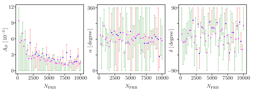
Figure 1: The marginalized $1\sigma$ constraints on the amplitude $A_{D}$, the right ascension $\alpha$, and the declination $\delta$ of the dipole, by using various simulated datasets consisting of $N_{\rm FRB}$ FRBs generated with a preset dipole $A_{D}^{\rm fid}=10^{-3}$, $\alpha_{\rm fid}=150^{\circ}$, and $\delta_{\rm fid}=10^{\circ}$. The green error bars with magenta means (the red error bars with blue means) indicate the cases that $A_{D}=0$ is consistent (inconsistent) with the simulated FRB dataset in the $1\sigma$ region, respectively. Note that $A_{D}$ is given in units of $10^{-3}$. See the text for details.

III Testing the cosmic anisotropy with the simulated FRBs

III.1 Generating the simulated FRB datasets with a preset direction

In fact, the methodology to simulate FRBs given in Sec. II is statistically isotropic. Although there exists variance in $\rm DM_{E}$ for different lines of sight, it is actually statistical noise due to random fluctuations, and hence there is no preferred direction in the simulated FRB datasets indeed.

There exist various methods to generate the simulated datasets with a preset direction in the literature (e.g. Deng:2018yhb ; Lin:2016jqp ; Cai:2017aea ; Lin:2018azu ). A simple way is to directly put a dipole with the preset direction into the simulated data under consideration. In our case, the simulated data of FRB is the extragalactic (or excess) dispersion measure $\rm DM_{E}$, similar to the cases considered in e.g. Yang:2016zbm . Since the simulated $\rm DM_{E}$ given in Eq. (19) is statistically isotropic in fact, we refer to it as $\rm DM_{E}^{iso}$ instead. The simulated $\rm DM_{E}$ with a preset direction $\hat{n}_{\rm fid}$ is given by

$${\rm DM_{E}}={\rm DM_{E}^{iso}}\left[\,1+A_{D}^{\rm fid}\left(\hat{n}_{\rm fid}\cdot\hat{p}\right)\,\right]\,,$$ (20)

where $\rm DM_{E}^{iso}$ is actually the one given in Eq. (19), $A_{D}^{\rm fid}$ is the amplitude of the preset fiducial dipole. The preset fiducial dipole direction $\hat{n}_{\rm fid}$ in terms of the equatorial coordinates $(\alpha,\,\delta)$ is given by

$$\hat{n}_{\rm fid}=\cos(\delta_{\rm fid})\cos(\alpha_{\rm fid})\;\hat{\bf i}+\cos(\delta_{\rm fid})\sin(\alpha_{\rm fid})\;\hat{\bf j}+\sin(\delta_{\rm fid})\;\hat{\bf k}\,,$$ (21)

where $\hat{\bf i}$, $\hat{\bf j}$, $\hat{\bf k}$ are the unit vectors along the axes of Cartesian coordinate system, and $\alpha_{\rm fid}$, $\delta_{\rm fid}$ are the right ascension (ra), declination (dec) of the preset fiducial dipole direction, respectively. The position of the $i$-th simulated data point with the equatorial coordinates $(\alpha_{i},\,\delta_{i})$ is given by

$$\hat{p}_{i}=\cos(\delta_{i})\cos(\alpha_{i})\;\hat{\bf i}+\cos(\delta_{i})\sin(\alpha_{i})\;\hat{\bf j}+\sin(\delta_{i})\;\hat{\bf k}\,.$$ (22)

Note that in the present work, we arbitrarily adopt the preset fiducial dipole direction as $\alpha_{\rm fid}=150^{\circ}$ and $\delta_{\rm fid}=10^{\circ}$. On the other hand, the amplitude of the preset fiducial dipole $A_{D}^{\rm fid}$ will be specified in the particular simulation (see below).

Let us briefly describe the main steps to generate the simulated FRB datasets with a preset direction:

1. Assign a random number uniformly taken from $[\,0^{\circ},\,360^{\circ})$ to the simulated FRB as its right ascension $\alpha_{i}\,$, and assign a random number uniformly taken from $[\,-90^{\circ},\,+90^{\circ}\,]$ to this simulated FRB as its declination $\delta_{i}\,$.

2. Assign a random redshift $z_{i}\leq 3$ from the distribution in Eq. (18) to this simulated FRB.

3. Calculate ${\rm DM_{E,\,{\it i}}^{iso}=DM_{IGM,\,{\it i}}+DM_{HG,\,loc,\,{\it i}}}/(1+z_{i})$ as described in Sec. II.

4. Generate $\rm DM_{E,\,{\it i}}$ for this simulated FRB by using Eqs. (20)$\,\sim\,$(22) with a preset dipole direction.

5. Generate the error $\sigma_{{\rm E},\,i}=\big{\{}\sigma_{\rm IGM}^{2}+\left[\,\sigma_{\rm HG,\,loc}/(1+z_{i})\,\right]^{2}\big{\}}^{1/2}$ for this FRB data point.

6. Repeat the above steps for $N_{\rm FRB}$ times to generate $N_{\rm FRB}$ simulated FRBs.

The formatted output data file for the simulated FRBs contains $N_{\rm FRB}$ rows of $\left\{\alpha_{i},\,\delta_{i},\,z_{i},\,{\rm DM_{E,\,{\it i}}},\,\sigma_{{\rm E},\,i}\right\}$. Once a simulated FRB dataset has been generated, one should forget everything used to generate it, including all the fiducial cosmology, parameters, and preset dipole. One should pretend to deal with it as a real “ observational ” dataset blindly.

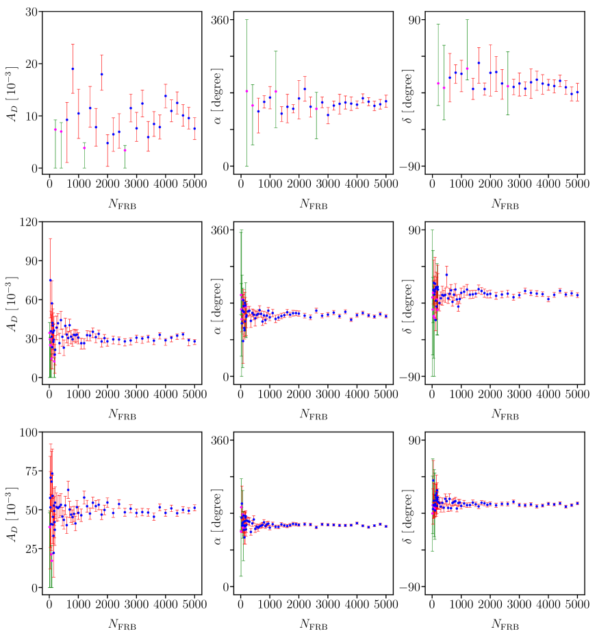
Figure 2: The same as in Fig. 1, except for $A_{D}^{\rm fid}=0.01$ (top panels), $0.03$ (middle panels) and $0.05$ (bottom panels), respectively. See the text for details.

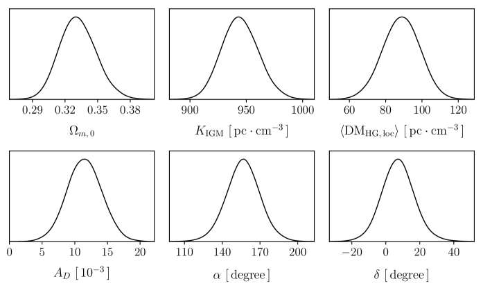
Figure 3: The marginalized probability distributions of all the 6 free model parameters $\Omega_{m,\,0}$, $K_{\rm IGM}$, $\langle{\rm DM_{HG,\,loc}}\rangle$, $A_{D}$, $\alpha$, $\delta$, by using 2800 FRBs simulated with $A_{D}^{\rm fid}=0.01$. Note that $A_{D}$ is given in units of $10^{-3}$. See the text and the top panels of Fig. 2 for details.

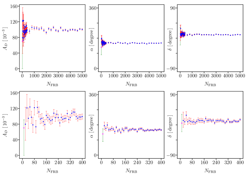
Figure 4: The same as in Fig. 1, except for $A_{D}^{\rm fid}=0.1$. The bottom panels are actually the foreparts $N_{\rm FRB}\leq 400$ of the top panels. See the text for details.

III.2 Testing the cosmic anisotropy with the simulated FRB datasets

Here, we try to test the possible cosmic anisotropy with the simulated FRB datasets. We assume that the universe can be theoretically described by a flat $\Lambda$CDM model, and the corresponding dimensionless Hubble parameter $E(z)$ is given in Eq. (14). We consider the extragalactic (or excess) dispersion measure $\rm DM_{E}$ with a possible dipole,

$${\rm DM_{E}^{th}}=\langle{\rm DM_{E}}\rangle\left[\,1+A_{D}\left(\hat{n}\cdot\hat{p}\right)\,\right]\,,$$ (23)

where $\langle{\rm DM_{E}}\rangle=\langle{\rm DM_{IGM}}\rangle+\langle{\rm DM_{HG,\,loc}}\rangle/(1+z)$, and $\langle{\rm DM_{IGM}}\rangle$ is given in Eq. (12). The dipole direction $\hat{n}$ in terms of the equatorial coordinates $(\alpha,\,\delta)$ is given by

$$\hat{n}=\cos(\delta)\cos(\alpha)\;\hat{\bf i}+\cos(\delta)\sin(\alpha)\;\hat{\bf j}+\sin(\delta)\;\hat{\bf k}\,.$$ (24)

There are 6 free model parameters, namely $\Omega_{m,\,0}$, $K_{\rm IGM}$, $\langle{\rm DM_{HG,\,loc}}\rangle$, $A_{D}$, $\alpha$ and $\delta$. The constraints on these 6 free model parameters can be obtained by using the simulated FRB dataset. The corresponding $\chi^{2}$ is given by

$$\chi^{2}\left(\Omega_{m,\,0},\,K_{\rm IGM},\,\langle{\rm DM_{HG,\,loc}}\rangle,\,A_{D},\,\alpha,\,\delta\right)=\sum_{i}\frac{\left({\rm DM}_{{\rm E},\,i}-{\rm DM_{E}^{th}}\right)^{2}}{\sigma_{{\rm E},\,i}^{2}}\,.$$ (25)

In the following, we use the Markov Chain Monte Carlo (MCMC) code CosmoMC Lewis:2002ah to this end. Noting that $A_{D}\left(\hat{n}\cdot\hat{p}\right)=-A_{D}\left(-\hat{n}\cdot\hat{p}\right)$ in Eq. (23), a positive $A_{D}$ with a direction $\hat{n}$ is equivalent to a negative $A_{D}$ with an opposite direction $-\hat{n}$. Therefore, in this work, without loss of generality, we require $A_{D}\geq 0$ as prior when running CosmoMC.

It is of interest to see how many FRBs (at least) are required to find a possible cosmic anisotropy. At first, we consider a tiny cosmic anisotropy represented by a dipole with $A_{D}^{\rm fid}=0.001$. Adopting this $A_{D}^{\rm fid}$, we generate a series of simulated FRB datasets consisting of $N_{\rm FRB}=200$, 400, 600, …, 10000 FRBs, respectively. For each simulated FRB dataset, we can obtain the constraints on the 6 free model parameters mentioned above, by using the MCMC code CosmoMC. We focus on the parameters related to the dipole, namely $A_{D}$, $\alpha$ and $\delta$. We present the marginalized $1\sigma$ constraints on these 3 dipole parameters versus $N_{\rm FRB}$ in Fig. 1. The green error bars with magenta means (the red error bars with blue means) indicate the cases that $A_{D}=0$ is consistent (inconsistent) with the simulated FRB dataset in the $1\sigma$ region, respectively. If $A_{D}=0$ is consistent with the “ observational ” dataset, it means that no preferred direction is found. Unfortunately, from Fig. 1, we see that even up to the case of $N_{\rm FRB}=10000$, $A_{D}=0$ is still consistent with the simulated FRB dataset. On the other hand, the constraints on the dipole direction $(\alpha,\,\delta)$ are fairly loose. Even in the cases that $A_{D}=0$ is not included in the $1\sigma$ region, the “ found ” $1\sigma$ angular regions are too wide to say that a preferred direction is really found. Thus, FRBs are not competent to find the tiny cosmic anisotropy with a dipole amplitude of ${\cal O}(10^{-3})$. We will come back to this issue in the next subsection (Sec. III.3).

We turn to the case of a larger cosmic anisotropy represented by a dipole with $A_{D}^{\rm fid}=0.01$. Adopting this $A_{D}^{\rm fid}$, we generate a series of simulated FRB datasets consisting of $N_{\rm FRB}=200$, 400, 600, …, 5000 FRBs, respectively. Similarly, we present the marginalized $1\sigma$ constraints on the dipole parameters $A_{D}$, $\alpha$, $\delta$ versus $N_{\rm FRB}$ in the top panels of Fig. 2. It is easy to see that in all cases of $N_{\rm FRB}\geq 2800$, a non-zero $A_{D}$ beyond $1\sigma$ region can be found, while the $1\sigma$ constraints on $\alpha$ and $\delta$ are also tight. Therefore, at least 2800 FRBs are competent to find the cosmic anisotropy with $A_{D}^{\rm fid}=0.01$. More FRBs lead to tighter constraints on the cosmic anisotropy. It is of interest to see also the constraints on the other free model parameters. In Fig. 3, we present the marginalized probability distributions of all the 6 free model parameters for the case of $N_{\rm FRB}=2800$. Obviously, the constraints on all the 6 parameters are consistent with the fiducial ones used to generate this simulated FRB dataset. For conciseness, we choose not to show the constraints on all the 6 parameters again in the rest of this paper, since we are mainly interested in the 3 parameters related to the cosmic anisotropy, namely $A_{D}$, $\alpha$ and $\delta$.

For the case of $A_{D}^{\rm fid}=0.03$, we also present the marginalized $1\sigma$ constraints on the dipole parameters $A_{D}$, $\alpha$, $\delta$ versus $N_{\rm FRB}=10$, 20, 30, …, 180, 190, 200, 250, 300, 350, 400, …, 950, 1000, 1100, …, 2000, 2200, …, 5000 in the middle panels of Fig. 2. We see that in all cases of $N_{\rm FRB}\geq 190$, a non-zero $A_{D}$ beyond $1\sigma$ region can be found, while the $1\sigma$ constraints on $\alpha$ and $\delta$ are fairly tight. Obviously, for all cases of $N_{\rm FRB}\geq 190$, the constraints on the parameters $A_{D}$, $\alpha$, $\delta$ are well consistent with the fiducial ones used to generate the simulated FRB datasets. Therefore, at least 190 FRBs are competent to find the cosmic anisotropy with $A_{D}^{\rm fid}=0.03$.

Similarly, we present the corresponding results for the case of $A_{D}^{\rm fid}=0.05$ in the bottom panels of Fig. 2. Obviously, the constraints on the parameters $A_{D}$, $\alpha$, $\delta$ become tighter (especially for the angular parameters $\alpha$ and $\delta$). In all cases of $N_{\rm FRB}\geq 100$, a non-zero $A_{D}$ beyond $1\sigma$ region can be found, while the $1\sigma$ constraints on $\alpha$ and $\delta$ are fairly tight. In other words, at least 100 FRBs are competent to find the cosmic anisotropy with $A_{D}^{\rm fid}=0.05$.

Finally, we consider a large cosmic anisotropy with $A_{D}^{\rm fid}=0.1$, and present the corresponding results in Fig. 4. To see clearly, we also enlarge the parts of $N_{\rm FRB}\leq 400$ in the bottom panels of Fig. 4. For such a big cosmic anisotropy, it is easy to find the non-zero dipole with high precision by using very few FRBs with known redshifts. In fact, at least 20 FRBs with known redshifts are competent to find the cosmic anisotropy with $A_{D}^{\rm fid}=0.1$. However, by now, there are only a few FRBs (e.g. the repeater FRB 121102) with identified redshifts, and hence the published FRBs to date are still not enough. We expect that such a big cosmic anisotropy can be ruled out by using only a few tens of FRBs with known redshifts in the near future.

Figure 5: The marginalized $1\sigma$ constraints on the amplitude $A_{D}$, the right ascension $\alpha$, and the declination $\delta$ of the dipole, by using 1000 simulated datasets consisting of $N_{\rm FRB}=200$ FRBs generated without a preset dipole (namely $A_{D}^{\rm fid}=0$). The green error bars with magenta means (the red error bars with blue means) indicate the cases that $A_{D}=0$ is consistent (inconsistent) with the simulated FRB dataset in the $1\sigma$ region, respectively. Note that $A_{D}$ is given in units of $10^{-3}$. See the text for details.

III.3 Ratio of pseudo anisotropic signals from the statistical noise

An important question is how reliable are the above results? In fact, pseudo anisotropic signals from the statistical noise due to random fluctuations are possible. Here, we would like to test this possibility in more details.

The key is to find the pseudo anisotropic signal in the simulated FRB datasets generated without a preset anisotropy (namely $A_{D}^{\rm fid}=0$). Noting that at least 190 FRBs are competent to find a cosmic dipole with amplitude $\sim 0.03$ as mentioned above, we randomly generate 1000 simulated datasets consisting of $N_{\rm FRB}=200$ FRBs without a preset dipole (namely $A_{D}^{\rm fid}=0$). For each simulated dataset consisting of $N_{\rm FRB}=200$ FRBs, we can obtain the constraints on the 6 free model parameters, following the same procedures used in the previous subsection, as if $A_{D}^{\rm fid}\not=0$. In Fig. 5, we present the marginalized $1\sigma$ constraints on the 3 dipole parameters for each simulated dataset consisting of $N_{\rm FRB}=200$ FRBs. In all the 1000 simulations, there are 212 simulations having a non-zero $A_{D}$ beyond $1\sigma$ region, as shown by the red error bars with blue means in the left panel of Fig. 5. However, a non-zero $A_{D}$ is not enough to say that a preferred direction has been found. In fact, many of them correspond to a very wide $1\sigma$ angular region, namely the $1\sigma$ constraints on the angular parameters $\alpha$ and $\delta$ are very loose, as shown by the long red error bars with blue means in the middle and right panels of Fig. 5. In some cases, the corresponding direction can be the whole sky or a half sky. Therefore, we cannot say that a preferred direction has been really found. On the contrary, we would like to mention the fairly tight $1\sigma$ constraints on $\alpha$ and $\delta$ in the simulations generated with a no-zero dipole ($A_{D}^{\rm fid}\not=0$), as shown in the the middle and right panels of Figs. 2 and 4. Here, we propose a fairly loose direction criterion, namely the $1\sigma$ range (upper bound minus lower bound) of the right ascension $\alpha$ should be $\leq 180^{\circ}$, and the $1\sigma$ range (upper bound minus lower bound) of the declination $\delta$ should be $\leq 90^{\circ}$. Noting that the value ranges of $\alpha$ and $\delta$ are $[\,0^{\circ},\,360^{\circ})$ and $[\,-90^{\circ},\,+90^{\circ}\,]$ respectively, this direction criterion is indeed fairly loose. Actually, in the 212 simulations with a non-zero $A_{D}$ beyond $1\sigma$ region mentioned above, only 115 simulations can pass this loose direction criterion. However, only 30 of these 115 simulations have a $1\sigma$ upper bound on $A_{D}$ higher than $0.03$ (please remember that 200 FRBs are competent to find a cosmic dipole with amplitude $\sim 0.03$ as mentioned above). In other words, when we report a cosmic dipole with amplitude $\sim 0.03$ by using 200 FRBs, there are only 30 pseudo anisotropic signals from the statistical noise in 1000 simulations. The ratio of pseudo anisotropic signals from the statistical noise is around $30/1000=3\%$, which is acceptable in fact. Note that the ratio of pseudo anisotropic signals will significantly decrease with more FRBs (for example, when one reports a cosmic dipole with amplitude $\sim 0.03$ by using $500+$ FRBs with known redshifts).

Similarly, noting that at least 2800 FRBs are competent to find a cosmic dipole with amplitude $\sim 0.01$ as mentioned above, we randomly generate 1000 simulated datasets consisting of $N_{\rm FRB}=3000$ FRBs without a preset dipole (namely $A_{D}^{\rm fid}=0$). In Fig. 6, we present the marginalized $1\sigma$ constraints on the 3 dipole parameters for each simulated dataset consisting of $N_{\rm FRB}=3000$ FRBs. In all the 1000 simulations, there are 218 simulations having a non-zero $A_{D}$ beyond $1\sigma$ region, as shown by the red error bars with blue means in the left panel of Fig. 6. Again, many of them correspond to a very wide $1\sigma$ angular region, namely the $1\sigma$ constraints on the angular parameters $\alpha$ and $\delta$ are very loose, as shown by the long red error bars with blue means in the middle and right panels of Fig. 6. In these 218 simulations with a non-zero $A_{D}$ beyond $1\sigma$ region mentioned above, only 133 simulations can pass the loose direction criterion proposed above. However, only 3 of these 133 simulations have a $1\sigma$ upper bound on $A_{D}$ higher than $0.01$ (please remember that 3000 FRBs are competent to find a cosmic dipole with amplitude $\sim 0.01$ as mentioned above). Thus, when we report a cosmic dipole with amplitude $\sim 0.01$ by using 3000 FRBs, the ratio of pseudo anisotropic signals from the statistical noise is around $3/1000=0.3\%$.

Through the above two concrete examples, we show that the results obtained in Sec. III.2 are reliable, because the ratio of pseudo anisotropic signals from the statistical noise is fairly low. It is worth noting that the available FRBs with known redshift will be numerous in the coming years, as mentioned in Sec. I. With numerous FRBs, it is reasonable to expect that the ratio of pseudo anisotropic signals from the statistical noise will become much less than $0.1\%$.

As a byproduct, from the above simulations, we can also understand why FRBs are not competent to find the tiny cosmic anisotropy with a dipole amplitude of ${\cal O}(10^{-3})$, even by using 10000 FRBs with known redshifts, as mentioned in Sec. III.2. As shown in the left panels of Figs. 5 and 6, most of the means (magenta and blue points) of $A_{D}$ from the statistical noise are about ${\cal O}(10^{-3})$. Therefore, even a real anisotropic signal of ${\cal O}(10^{-3})$ exsists, it will be hidden behind the statistical noise.

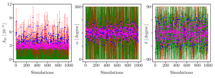
Figure 6: The same as in Fig. 5, except for 1000 simulated datasets consisting of $N_{\rm FRB}=3000$ FRBs generated without a preset dipole (namely $A_{D}^{\rm fid}=0$). See the text for details.

IV Concluding remarks

In the recent years, the field of FRBs is thriving and growing rapidly. It is of interest to study cosmology by using FRBs with known redshifts. In the present work, we try to test the possible cosmic anisotropy with the simulated FRBs. We find that at least 2800, 190, 100 FRBs are competent to find the cosmic anisotropy with a dipole amplitude 0.01, 0.03, 0.05, respectively. Unfortunately, even 10000 FRBs are not competent to find the tiny cosmic anisotropy with a dipole amplitude of ${\cal O}(10^{-3})$. On the other hand, at least 20 FRBs with known redshifts are competent to find the cosmic anisotropy with a dipole amplitude 0.1. We expect that such a big cosmic anisotropy can be ruled out by using only a few tens of FRBs with known redshifts in the near future.

Some remarks are in order. First, we find that so far FRBs are not competent to find the tiny cosmic anisotropy with a dipole amplitude of ${\cal O}(10^{-3})$. In fact, it is easy to imagine that even the cosmological principle is broken, the violation cannot be too large. For example, the Union2.1 sample consisting of 580 SNIa suggests that there is a cosmic anisotropy with a dipole amplitude around $1.2\times 10^{-3}$ Lin:2016jqp . No cosmic anisotropy has been found in the JLA sample consisting of 740 SNIa Deng:2018yhb ; Lin:2015rza ; Chang:2017bbi and the latest Pantheon sample consisting of 1048 SNIa Deng:2018jrp ; Sun:2018cha ; Andrade:2018eta . Our results obtained here suggest that FRBs can be used to find or rule out the cosmic anisotropy with a dipole amplitude $\gtrsim 10^{-2}$, but cannot be used to find or rule out the cosmic anisotropy with a dipole amplitude $\lesssim{\cal O}(10^{-3})$.

Second, as mentioned in Sec. III.3, a possible cosmic anisotropy of ${\cal O}(10^{-3})$ will be hidden behind the pseudo anisotropic signals of ${\cal O}(10^{-3})$ from the statistical noise. Thus, it is necessary to reduce the statistical noise. As mentioned in Sec. II, the main cause of this considerable statistical noise is the large $\sigma_{\rm IGM}\sim 100\;{\rm pc\hskip 2.40005ptcm^{-3}}$ McQuinn:2013tmc due to the IGM plasma density fluctuations. On the other hand, actually this large $\sigma_{\rm IGM}\sim 100\;{\rm pc\hskip 2.40005ptcm^{-3}}$ is also the cause of the relatively large uncertainty when one uses FRBs to constrain other cosmological parameters (see e.g. Deng:2013aga ; Yang:2016zbm ; Gao:2014iva ; Zhou:2014yta ; Yu:2017beg ; Yang:2017bls ; Wei:2018cgd ; Li:2017mek ; Jaroszynski:2018vgh ; Madhavacheril:2019buy ; Wang:2018ydd ; Walters:2017afr ). To obtain tight constraints, one has to combine FRBs with other cosmological probes such as SNIa, baryon acoustic oscillations (BAO), CMB, and GRBs. Therefore, it is of interest to reduce this large $\sigma_{\rm IGM}$ in FRBs cosmology.

Third, the present work can be extended to more general cases. For example, we consider a flat $\Lambda$CDM cosmology here, and it can be generalized to other cosmological models such as $w$CDM and CPL. On the other hand, here we only consider FRBs at redshift $z\leq 3$ to ensure that hydrogen and helium are both fully ionized. However, we can extend to high redshift $z\leq 6$. In the redshift range $3<z<6$, although helium is not fully ionized while hydrogen is fully ionized, the relevant calculations still can be carried out (see e.g. Gao:2014iva ). Actually, it is expected that FRBs are detectable up to redshift $z\sim 15$ in e.g. Zhang:2018fxt . Although it is really a challenge to calculate DM at high redshift $z>6$, FRBs at high redshifts are fairly valuable in cosmology. Here, let us further discuss this issue in more details. If we consider a broader range of redshift e.g. $z\leq 6$ for FRBs (we thank the anonymous referee 1 for pointing out this issue), helium is not fully ionized at $z>3$. In this case, $\chi_{e,\,\rm He}(z)$ becomes a piecewise function Gao:2014iva

$$\chi_{e,\,\rm He}(z)=\left\{\begin{array}[]{l}1\,,\quad\quad{\rm for}\quad z\leq 3\,,\\[5.69054pt] 0.025\,z^{3}-0.244\,z^{2}+0.513\,z+1.006\,,\quad\quad{\rm for}\quad 3<z\leq 6\,.\end{array}\right.$$ (26)

If we extend to higher redshift $z>6$, hydrogen and helium are both not fully ionized, and hence $\chi_{e,\,\rm H}(z)$ and $\chi_{e,\,\rm He}(z)$ should be both piecewise functions, similar to Eq. (26). On the other hand, the fraction of baryon mass in the intergalactic medium $f_{\rm IGM}$ might be not a constant at high redshifts. In fact, the varying $f_{\rm IGM}(z)$ has been considered in the literature (e.g. Li:2019klc ; Wei:2019uhh ; Qiang:2020vta ). In particular, it is reasonable to consider a linear parameterization with respect to the scale factor $a$, namely Li:2019klc ; Qiang:2020vta

$$f_{\rm IGM}(z)=f_{\rm IGM,\,0}\,(1+\beta\,(1-a))=f_{\rm IGM,\,0}\,(1+\beta\,z/(1+z))\,.$$ (27)

So, if we consider FRBs at high redshifts $z>3$, both $f_{e}$ and $f_{\rm IGM}$ might be functions of redshift $z$, and hence the calculation of $\langle{\rm DM_{IGM}}\rangle$ should be changed accordingly (nb. Eqs. (12) and (13)).

Fourth, we stress that our current results do not completely exclude the possibility that FRBs can become competent in the future to find or rule out the tiny cosmic anisotropy with a dipole amplitude $\lesssim{\cal O}(10^{-3})$. As mentioned in Sec. I, thousands FRB events per day over the entire sky are expected (see e.g. Keane:2018jqo ; Bhandari:2017qrj ; Amiri:2019qbv ). So, numerous FRBs (say, $10^{6}$ FRBs, significantly more than 10000 FRBs considered in this work) might be available in the future. On the other hand, the statistical noise of FRBs (especially $\sigma_{\rm IGM}$) might be significantly reduced by the help of future developments (say, FRBs lensing and so on). And, many FRBs at high redshift $3<z<6$ might be also available in the future. Although FRBs with known redshift are very few by now, they will soon become numerous in the near future. In fact, very recently a non-repeating FRB 180924 Bannister2019 has been localized to a massive galaxy at redshift 0.3214 by using ASKAP. Another non-repeating FRB 190523 Ravi:2019alc has been localized to a few-arcsecond region containing a single massive galaxy at redshift 0.66 by using DSA-10. Actually, several projects designed to detect and localize FRBs with arcsecond accuracy in real time are under constriction/proposition, for example, DSA-10 DSA-10 and DSA-2000 DSA-2000 . Thus, it is reasonable to expect that most of future FRBs are available with known redshifts. In summary, it is still possible that FRBs can become competent in the future to find or rule out the tiny cosmic anisotropy with a dipole amplitude $\lesssim{\cal O}(10^{-3})$, by the help of future developments mentioned above.

Fifth, in this work we assume that the redshift distribution of FRBs takes a form similar to the one of GRBs, namely Eq. (18). However, this might be changed as the number of FRBs increases in the future (we thank the anonymous referee 1 for pointing out this issue). In fact, there exist some different redshift distributions for FRBs in the literature. For example, two types of redshift distributions for FRBs have been proposed in Munoz:2016tmg , namely

$$P(z)\propto\frac{\chi^{2}(z)}{\left(1+z\right)H(z)}\,\exp\left(-\frac{d_{L}^{\,2}(z)}{2\,d_{L}^{\,2}(z_{\rm cut})}\right)\,,\quad{\rm or}\quad P(z)\propto\frac{\dot{\rho}_{\ast}(z)\,\chi^{2}(z)}{\,\left(1+z\right)H(z)}\,\exp\left(-\frac{d_{L}^{\,2}(z)}{2\,d_{L}^{\,2}(z_{\rm cut})}\right)\,,$$ (28)

where $\chi(z)=d_{L}(z)/(1+z)=c\int_{0}^{z}d\tilde{z}/H(\tilde{z})$ is the comoving distance, and $d_{L}(z)$ is the luminosity distance. $\dot{\rho}_{\ast}(z)$ corresponds to the star-formation history (SFH). Gaussian cutoff at $z_{\rm cut}$ is introduced to represent an instrumental signal-to-noise threshold. Of course, other types of redshift distributions for FRBs are also possible. However, we argue that different redshift distributions of FRBs do not significantly change the results obtained in this work. As shown in Eqs. (20)–(25), the dipole anisotropy is mainly related to the positions of FRBs in the sky (namely right ascension $\alpha$ and declination $\delta$), rather than their redshifts. Thus, it is reasonable to expect that the redshift distribution of FRBs will not play an important role in testing the cosmic anisotropy.

Sixth, as mentioned in the beginning of Sec. II, we use $\rm DM_{E}$ instead of $\rm DM_{obs}$ to study the FRB cosmology for convenience following e.g. Yang:2016zbm ; Yang:2017bls . Actually, the difference between them is the contribution from Milky Way, $\rm DM_{MW}$. For a well-localized FRB, the corresponding $\rm DM_{MW}$ can be known by using the NE2001 model Cordes:2003ik ; Cordes:2002wz or the YMW16 model YMW16 for the galactic distribution of free electrons and its fluctuations constructed from the known pulsar DM data. It is worth noting that we have not neglected $\rm DM_{MW}$ in fact (although $\rm DM_{MW}$ is usually small with respect to $\rm DM_{obs}$). Instead, we just subtract $\rm DM_{MW}$ from $\rm DM_{obs}$ to introduce $\rm DM_{E}=DM_{obs}-DM_{MW}$, as in Eq. (6). Since there is no theoretical model for $\rm DM_{obs}$, we instead calculate $\rm DM_{E}\equiv DM_{obs}-DM_{MW}=DM_{IGM}+DM_{HG}$ in the simulations because $\rm DM_{obs}=DM_{MW}+DM_{IGM}+DM_{HG}$ (see Eq. (5)). Accordingly, the uncertainty of $\rm DM_{E}$ is given by $\sigma_{\rm E}=(\sigma_{\rm IGM}^{2}+\sigma_{\rm HG}^{2})^{1/2}=\{\,\sigma_{\rm IGM}^{2}+[\,\sigma_{\rm HG,\,loc}/(1+z)\,]^{2}\,\}^{1/2}$ in the simulations, as mentioned at the end of Sec. III.1. Of course, one can also calculate $\sigma_{\rm E}$ by using the uncertainties of $\rm DM_{obs}$ and $\rm DM_{MW}$, since $\rm DM_{E}=DM_{obs}-DM_{MW}$. Although the uncertainty of $\rm DM_{obs}$ is usually small, $\sigma_{\rm E}$ is not so small because we have not neglected $\rm DM_{MW}$ and hence the uncertainty of $\rm DM_{MW}$ should be also taken into account. Since $\rm DM_{MW}$ is known by using the NE2001 model Cordes:2003ik ; Cordes:2002wz or the YMW16 model YMW16 for the galactic distribution of free electrons and its fluctuations, it is model-dependent in some sense, while its uncertainty $\sigma_{\rm MW}$ is not small in fact (on the other hand, one should be aware of the considerable difference between the NE2001 and YMW16 models). Because we are mainly concerned about the cosmological information carried by $\rm DM_{IGM}$, while it is hard to construct $\rm DM_{MW}$ from the NE2001 or YMW16 models and there is no theoretical model for $\rm DM_{obs}$, in this work we choose to simulate $\rm DM_{E}$ by using $\rm DM_{IGM}$ and $\rm DM_{HG}$, as well as their uncertainties.

Seventh, we have paid attention to the possible dipole with amplitude of ${\cal O}(10^{-3})$ or ${\cal O}(10^{-2})$ in this work (we thank the anonymous referee 2 for pointing out this issue). In the literature, the claimed cosmic dipole amplitude is $A_{D}\sim{\cal O}(10^{-3})$ or ${\cal O}(10^{-2})$ by using SNIa (see e.g. Mariano:2012wx ; Cai:2011xs ; Yang:2013gea ; Chang:2014nca ), SNIa+GRBs (see e.g. Wang:2014vqa ; Chang:2014jza ), radio galaxies (see e.g. Bengaly:2017slg ), and so on. As is well known, the dipole in the CMB temperature map is also $A_{D}\sim{\cal O}(10^{-3})$ (see e.g. Aghanim:2013suk ). These results in the literature motivate us to consider the possible dipole in FRBs with amplitude of similar order of magnitude.

Eighth, we would like to emphasize the physical significance of a possible cosmic dipole (we thank the anonymous referee 2 for pointing out this issue). Here we are mainly interested in probing differential expansion of space, as in e.g. Antoniou:2010gw ; Cai:2011xs . A cosmic dipole gives a hint of one (or more) preferred axis in the universe. Actually, the preferred axis is possible in various exotic cosmological models. For example, in the well-known Gödel solution Godel:1949ga (see also e.g. Li:2016nnn and references therein) of Einstein’s field equations, the universe is rotating around an axis. As is well known, the time travel is possible in the Gödel universe. Besides the Gödel universe, in the Finsler universe Li:2015uda and most of Bianchi type I$\,\sim\,$IX universes Bianchi , the cosmic anisotropy is also possible. So, if a cosmic dipole is confirmed, it will force us to consider such kind of exotic models seriously.

Ninth, it is of interest to discuss the potential astrophysical systematics contaminating the signal. In particular, one might speculate that observational systematic errors could create an apparent dipole signal for FRBs, for example, if more high redshift FRBs are observable in one part of the sky as compared to another due to foreground contamination (we thank the anonymous referee 2 for pointing out this issue). Here we argue that such kind of systematics might be fairly minor. It is useful to consult with the cases of SNIa. The Pantheon sample Scolnic:2017caz ; Pantheondata ; Pantheonplugin is the largest spectroscopically confirmed SNIa sample to date, which consists of 1048 SNIa. As is shown in Fig. 1 of Deng:2018jrp (and its Sec. 2), more than one half of 1048 Pantheon SNIa are located in a small region of the southern sky (because of some unknown reasons to our knowledge). However, no evidence for the cosmic dipole is found in the Pantheon SNIa sample Deng:2018jrp . In fact, it is the same for the JLA sample consisting of 740 SNIa Lin:2015rza ; Chang:2017bbi . In light of the cases of SNIa, we expect that the potential systematics mentioned above might be fairly minor.

Finally, the field of FRBs is growing rapidly. In fact, many new findings have been obtained after the (pre-)commissions of ASKAP and CHIME in 2018. Big breakthroughs in the coming years are expected. Therefore, FRBs cosmology might also have a promising future.

References

- (1) E. F. Keane, Nat. Astron. 2, 865 (2018) [arXiv:1811.00899].
- (2) D. R. Lorimer, Nat. Astron. 2, 860 (2018) [arXiv:1811.00195].
- (3) U. L. Pen, Nat. Astron. 2, 842 (2018) [arXiv:1811.00605].
- (4) S. R. Kulkarni, Nat. Astron. 2, 832 (2018) [arXiv:1811.00448].
- (5) S. Burke-Spolaor, Nat. Astron. 2, 845 (2018) [arXiv:1811.00194].
- (6) J. P. Macquart, Nat. Astron. 2, 836 (2018) [arXiv:1811.00197].
- (7) https:www.nature.com/collections/rswtktxcln
- (8) D. R. Lorimer et al., Science 318, 777 (2007) [arXiv:0709.4301].
- (9) D. Thornton et al., Science 341, no. 6141, 53 (2013) [arXiv:1307.1628].
- (10) D. J. Champion et al., Mon. Not. Roy. Astron. Soc. 460, no. 1, L30 (2016) [arXiv:1511.07746].
- (11) L. G. Spitler et al., Nature 531, 202 (2016) [arXiv:1603.00581].
- (12) S. P. Tendulkar et al., Astrophys. J. 834, no. 2, L7 (2017) [arXiv:1701.01100].
- (13) B. Marcote et al., Astrophys. J. 834, no. 2, L8 (2017) [arXiv:1701.01099].
- (14) S. Chatterjee et al., Nature 541, 58 (2017) [arXiv:1701.01098].
- (15) E. F. Keane et al., Nature 530, 453 (2016) [arXiv:1602.07477].
- (16) R. M. Shannon et al., Nature 562, 386 (2018).
- (17) M. Amiri et al., Nature 566, 230 (2019) [arXiv:1901.04524].
- (18) M. Amiri et al., Nature 566, 235 (2019) [arXiv:1901.04525].
-
(19)
E. Petroff et al.,
Publ. Astron. Soc. Austral. 33, e045 (2016)
[arXiv:1601.03547];
The up-to-date FRB Catalogue is available at http:www.frbcat.org - (20) G. B. Rybicki and A. P. Lightman, Radiative Processes in Astrophysics, John Wiley & Sons, Inc. (1979).
- (21) W. Deng and B. Zhang, Astrophys. J. 783, L35 (2014) [arXiv:1401.0059].
- (22) Y. P. Yang and B. Zhang, Astrophys. J. 830, no. 2, L31 (2016) [arXiv:1608.08154].
- (23) K. Ioka, Astrophys. J. 598, L79 (2003) [astro-ph/0309200].
- (24) S. Inoue, Mon. Not. Roy. Astron. Soc. 348, 999 (2004) [astro-ph/0309364].
- (25) S. Bhandari et al., Mon. Not. Roy. Astron. Soc. 475, no. 2, 1427 (2018) [arXiv:1711.08110].
- (26) B. Marcote and Z. Paragi, PoS EVN 2018, 013 (2019) [arXiv:1901.08541].
- (27) S. X. Yi, H. Gao and B. Zhang, Astrophys. J. 792, L21 (2014) [arXiv:1407.0348].
-
(28)
E. Platts et al.,
Phys. Rept. 821, 1 (2019)
[arXiv:1810.05836];
The up-to-date FRB Theory Catalogue is available at http:frbtheorycat.org - (29) H. Gao, Z. Li and B. Zhang, Astrophys. J. 788, 189 (2014) [arXiv:1402.2498].
- (30) B. Zhou, X. Li, T. Wang, Y. Z. Fan and D. M. Wei, Phys. Rev. D 89, 107303 (2014) [arXiv:1401.2927].
- (31) H. Yu and F. Y. Wang, Astron. Astrophys. 606, A3 (2017) [arXiv:1708.06905].
- (32) Y. P. Yang, R. Luo, Z. Li and B. Zhang, Astrophys. J. 839, no. 2, L25 (2017) [arXiv:1701.06465].
- (33) J. J. Wei, X. F. Wu and H. Gao, Astrophys. J. 860, no. 1, L7 (2018) [arXiv:1805.12265].
- (34) Z. X. Li, H. Gao, X. H. Ding, G. J. Wang and B. Zhang, Nat. Comm. 9, 3833 (2018) [arXiv:1708.06357].
- (35) M. Jaroszynski, Mon. Not. Roy. Astron. Soc. 484, no. 2, 1637 (2019) [arXiv:1812.11936].
- (36) M. S. Madhavacheril, N. Battaglia, K. M. Smith and J. L. Sievers, arXiv:1901.02418 [astro-ph.CO].
- (37) Y. K. Wang and F. Y. Wang, Astron. Astrophys. 614, A50 (2018) [arXiv:1801.07360].
- (38) A. Walters et al., Astrophys. J. 856, no. 1, 65 (2018) [arXiv:1711.11277].
- (39) D. W. Hogg et al., Astrophys. J. 624, 54 (2005) [astro-ph/0411197].
-
(40)
A. Hajian and T. Souradeep,
Phys. Rev. D 74, 123521 (2006)
[astro-ph/0607153];
T. R. Jaffe et al., Astrophys. J. 629, L1 (2005) [astro-ph/0503213]. - (41) R. R. Caldwell and A. Stebbins, Phys. Rev. Lett. 100, 191302 (2008) [arXiv:0711.3459].
-
(42)
G. Lemaître,
Annales de la Société Scientifique de Bruxelles A 53, 51 (1933),
see Gen. Rel. Grav. 29, 641 (1997) for English translation;
R. C. Tolman, Proc. Nat. Acad. Sci. 20, 169 (1934),
see Gen. Rel. Grav. 29, 935 (1997) for English translation;
H. Bondi, Mon. Not. Roy. Astron. Soc. 107, 410 (1947). - (43) X. P. Yan, D. Z. Liu and H. Wei, Phys. Lett. B 742, 149 (2015) [arXiv:1411.6218].
- (44) H. K. Deng and H. Wei, Phys. Rev. D 97, no. 12, 123515 (2018) [arXiv:1804.03087].
- (45) H. K. Deng and H. Wei, Eur. Phys. J. C 78, no. 9, 755 (2018) [arXiv:1806.02773].
- (46) K. Gödel, Rev. Mod. Phys. 21, 447 (1949).
-
(47)
S. L. Li, X. H. Feng, H. Wei and H. Lu,
Eur. Phys. J. C 77, no. 5, 289 (2017)
[arXiv:1612.02069];
W. J. Geng, S. L. Li, H. Lu and H. Wei, Phys. Lett. B 780, 196 (2018) [arXiv:1801.00009]. - (48) https:en.wikipedia.org/wiki/Bianchi-classification
-
(49)
X. Li, H. N. Lin, S. Wang and Z. Chang,
Eur. Phys. J. C 75, no. 5, 181 (2015)
[arXiv:1501.06738];
Z. Chang, S. Wang and X. Li, Eur. Phys. J. C 72, 1838 (2012) [arXiv:1106.2726]. -
(50)
K. Land and J. Magueijo,
Phys. Rev. Lett. 95, 071301 (2005)
[astro-ph/0502237];
K. Land and J. Magueijo, Mon. Not. Roy. Astron. Soc. 378, 153 (2007) [astro-ph/0611518];
K. Land and J. Magueijo, Mon. Not. Roy. Astron. Soc. 357, 994 (2005) [astro-ph/0405519]. - (51) W. Zhao and L. Santos, The Universe, no. 3, 9 (2015) [arXiv:1604.05484].
- (52) F. K. Hansen et al., Mon. Not. Roy. Astron. Soc. 354, 641 (2004) [astro-ph/0404206].
- (53) D. J. Schwarz and B. Weinhorst, Astron. Astrophys. 474, 717 (2007) [arXiv:0706.0165].
- (54) I. Antoniou and L. Perivolaropoulos, JCAP 1012, 012 (2010) [arXiv:1007.4347].
- (55) A. Mariano and L. Perivolaropoulos, Phys. Rev. D 86, 083517 (2012) [arXiv:1206.4055].
-
(56)
R. G. Cai and Z. L. Tuo,
JCAP 1202, 004 (2012)
[arXiv:1109.0941];
R. G. Cai, Y. Z. Ma, B. Tang and Z. L. Tuo, Phys. Rev. D 87, 123522 (2013) [arXiv:1303.0961]. - (57) W. Zhao, P. X. Wu and Y. Zhang, Int. J. Mod. Phys. D 22, 1350060 (2013) [arXiv:1305.2701].
- (58) X. Yang, F. Y. Wang and Z. Chu, Mon. Not. Roy. Astron. Soc. 437, 1840 (2014) [arXiv:1310.5211].
- (59) Z. Chang and H. N. Lin, Mon. Not. Roy. Astron. Soc. 446, 2952 (2015) [arXiv:1411.1466].
- (60) H. N. Lin, S. Wang, Z. Chang and X. Li, Mon. Not. Roy. Astron. Soc. 456, 1881 (2016) [arXiv:1504.03428].
- (61) Z. Chang et al., Mon. Not. Roy. Astron. Soc. 478, no. 3, 3633 (2018) [arXiv:1711.11321].
- (62) B. Javanmardi et al., Astrophys. J. 810, no. 1, 47 (2015) [arXiv:1507.07560].
- (63) H. N. Lin, X. Li and Z. Chang, Mon. Not. Roy. Astron. Soc. 460, no. 1, 617 (2016) [arXiv:1604.07505].
-
(64)
C. A. P. Bengaly, A. Bernui and J. S. Alcaniz,
Astrophys. J. 808, 39 (2015)
[arXiv:1503.01413];
U. Andrade et al., Phys. Rev. D 97, no. 8, 083518 (2018) [arXiv:1711.10536]. - (65) Z. Q. Sun and F. Y. Wang, Mon. Not. Roy. Astron. Soc. 478, no. 4, 5153 (2018) [arXiv:1805.09195].
- (66) U. Andrade et al., Astrophys. J. 865, no. 2, 119 (2018) [arXiv:1806.06990].
- (67) A. Meszaros et al., AIP Conf. Proc. 1133, 483 (2009) [arXiv:0906.4034].
- (68) J. S. Wang and F. Y. Wang, Mon. Not. Roy. Astron. Soc. 443, no. 2, 1680 (2014) [arXiv:1406.6448].
- (69) Z. Chang, X. Li, H. N. Lin and S. Wang, Mod. Phys. Lett. A 29, 1450067 (2014) [arXiv:1405.3074].
- (70) A. K. Singal, Astrophys. Space Sci. 357, no. 2, 152 (2015) [arXiv:1305.4134].
- (71) C. A. P. Bengaly, R. Maartens and M. G. Santos, JCAP 1804, 031 (2018) [arXiv:1710.08804].
- (72) Y. Zhou, Z. C. Zhao and Z. Chang, Astrophys. J. 847, no. 2, 86 (2017) [arXiv:1707.00417].
- (73) Z. Chang, H. N. Lin, Z. C. Zhao and Y. Zhou, Chin. Phys. C 42, 115103 (2018) [arXiv:1803.08344].
-
(74)
D. Hutsemekers et al.,
Astron. Astrophys. 441, 915 (2005)
[astro-ph/0507274];
D. Hutsemekers and H. Lamy, Astron. Astrophys. 367, 381 (2001) [astro-ph/0012182];
D. Hutsemekers et al., ASP Conf. Ser. 449, 441 (2011) [arXiv:0809.3088] - (75) V. Pelgrims, arXiv:1604.05141 [astro-ph.CO].
- (76) J. K. Webb et al., Phys. Rev. Lett. 82, 884 (1999) [astro-ph/9803165].
-
(77)
J. K. Webb et al.,
Phys. Rev. Lett. 87, 091301 (2001)
[astro-ph/0012539];
M. T. Murphy et al., Mon. Not. Roy. Astron. Soc. 327, 1208 (2001) [astro-ph/0012419]. - (78) J. P. Uzan, Living Rev. Rel. 14, 2 (2011) [arXiv:1009.5514].
- (79) J. D. Barrow, Ann. Phys. 19, 202 (2010) [arXiv:0912.5510].
-
(80)
H. Wei,
Phys. Lett. B 682, 98 (2009)
[arXiv:0907.2749];
H. Wei, X. P. Ma and H. Y. Qi, Phys. Lett. B 703, 74 (2011) [arXiv:1106.0102];
H. Wei, X. B. Zou, H. Y. Li and D. Z. Xue, Eur. Phys. J. C 77, no. 1, 14 (2017) [arXiv:1605.04571];
H. Wei and D. Z. Xue, Commun. Theor. Phys. 68, no. 5, 632 (2017) [arXiv:1706.04063]. - (81) J. A. King et al., Mon. Not. Roy. Astron. Soc. 422, 3370 (2012) [arXiv:1202.4758].
- (82) J. K. Webb et al., Phys. Rev. Lett. 107, 191101 (2011) [arXiv:1008.3907].
- (83) J. H. Taylor and J. M. Cordes, Astrophys. J. 411, 674 (1993).
-
(84)
R. N. Manchester et al.,
Astron. J. 129, 1993 (2005)
[astro-ph/0412641];
https:www.atnf.csiro.au/research/pulsar/psrcat/ - (85) J. M. Cordes and T. J. W. Lazio, astro-ph/0301598.
- (86) M. McQuinn, Astrophys. J. 780, L33 (2014) [arXiv:1309.4451].
- (87) A. A. Meiksin, Rev. Mod. Phys. 81, 1405 (2009) [arXiv:0711.3358].
- (88) G. D. Becker et al., Mon. Not. Roy. Astron. Soc. 410, 1096 (2011) [arXiv:1008.2622].
- (89) M. Fukugita, C. J. Hogan and P. J. E. Peebles, Astrophys. J. 503, 518 (1998) [astro-ph/9712020].
- (90) J. M. Shull, B. D. Smith and C. W. Danforth, Astrophys. J. 759, 23 (2012) [arXiv:1112.2706].
- (91) N. Aghanim et al., arXiv:1807.06209 [astro-ph.CO].
- (92) L. Shao et al., Astrophys. J. 738, 19 (2011) [arXiv:1104.5498].
- (93) R. G. Cai et al., Phys. Rev. D 97, no. 10, 103005 (2018) [arXiv:1712.00952].
- (94) H. N. Lin, J. Li and X. Li, Eur. Phys. J. C 78, no. 5, 356 (2018) [arXiv:1802.00642].
-
(95)
A. Lewis and S. Bridle,
Phys. Rev. D 66, 103511 (2002)
[astro-ph/0205436];
http:cosmologist.info/cosmomc/ - (96) B. Zhang, Astrophys. J. 867, no. 2, L21 (2018) [arXiv:1808.05277].
- (97) H. Ghodsi, S. Baghram and F. Habibi, JCAP 1710, 017 (2017) [arXiv:1609.08012].
-
(98)
P. Tiwari et al.,
Astropart. Phys. 61, 1 (2014)
[arXiv:1307.1947];
P. Tiwari and P. Jain, Mon. Not. Roy. Astron. Soc. 447, 2658 (2015) [arXiv:1308.3970];
P. Tiwari and P. Jain, Astron. Astrophys. 622, A113 (2019) [arXiv:1809.01270]. -
(99)
A. K. Singal,
Astrophys. J. 742, L23 (2011)
[arXiv:1110.6260];
M. Rubart and D. J. Schwarz, Astron. Astrophys. 555, A117 (2013) [arXiv:1301.5559]. - (100) K. W. Bannister et al., Science 365, no. 6453, 565 (2019) [arXiv:1906.11476].
- (101) V. Ravi et al., Nature 572, no. 7769, 352 (2019) [arXiv:1907.01542].
- (102) J. Kocz et al., Mon. Not. Roy. Astron. Soc. 489, no. 1, 919 (2019) [arXiv:1906.08699].
- (103) G. Hallinan et al., arXiv:1907.07648 [astro-ph.IM].
- (104) B. C. Andersen et al., Astrophys. J. 885, no. 1, L24 (2019) [arXiv:1908.03507].
- (105) R. G. Cai, T. B. Liu, S. J. Wang and W. T. Xu, JCAP 1909, 016 (2019) [arXiv:1905.01803].
- (106) Z. X. Li et al., Astrophys. J. 876, no. 2, 146 (2019) [arXiv:1904.08927].
- (107) J. J. Wei et al., JCAP 1909, 039 (2019) [arXiv:1907.09772].
- (108) J. B. Muñoz et al., Phys. Rev. Lett. 117, no. 9, 091301 (2016) [arXiv:1605.00008].
- (109) J. M. Cordes and T. J. W. Lazio, astro-ph/0207156.
- (110) J. M. Yao, R. N. Manchester and N. Wang, Astrophys. J. 835, 29 (2017) [arXiv:1610.09448].
-
(111)
N. Aghanim et al.,
Astron. Astrophys. 571, A27 (2014)
[arXiv:1303.5087];
Y. Akrami et al., arXiv:1807.06205 [astro-ph.CO]. - (112) D. M. Scolnic et al., Astrophys. J. 859, no. 2, 101 (2018) [arXiv:1710.00845].
-
(113)
The numerical data of the full Pantheon SNIa sample are available at
http:dx.doi.org/10.17909/T95Q4X
https:archive.stsci.edu/prepds/ps1cosmo/index.html -
(114)
The Pantheon plugin for CosmoMC is available at
https:github.com/dscolnic/Pantheon - (115) D. C. Qiang and H. Wei, JCAP 2004, 023 (2020) [arXiv:2002.10189].