Range separation: the divide between local structures and field theories

Abstract

This work presents parallel histories of the development of two modern theories of condensed matter: the theory of electron structure in quantum mechanics, and the theory of liquid structure in statistical mechanics. Comparison shows that key revelations in both are not only remarkably similar, but even follow along a common thread of controversy that marks progress from antiquity through to the present. This theme appears as a creative tension between two competing philosophies, that of short range structure (atomistic models) on the one hand, and long range structure (continuum or density functional models) on the other. The timeline and technical content are designed to build up a set of key relations as guideposts for using density functional theories together with atomistic simulation.

Key words: electronic structure, liquid state structure, density functional theory, Bayes’ theorem, vapor interface, molecular dynamics

Electronic address: davidrogers@usf.edu

Many of the most important scientific theories were forged out of controversy – like particles vs. waves, for which Democritus claimed (with his teacher, Leucippus of 5th century BC) that all things, including the soul, were made of particles, while Aristotle held to the Greek notion that there were continuous distributions of four or five elements.¹ It is telling to note that Aristotle’s objection was strongly biased by his notion that the continuum theory was elegant and beautiful, and does not require any regions of vacuum. In addition, his conception of kinetic equations were first order – like Brownian motion, Navier-Stokes, or the Dirac equation, but not second order like Newton’s or Schrödinger’s. Newton sided with Democritus. In 1738, Daniel Bernoulli first explained thermodynamic pressure using a model of independent atomic collisions. That theory was not scheduled to be widely adopted until the caloric theory (which postulated conservation of heat) was overthrown by James Joule in the 1850s. Wilhelm Ostwald was famously stubborn for refusing to accept the atomic nature of matter until the early 1900s, after Einstein’s theory of Brownian motion was confirmed by Jean Perrin’s experiment.

The working out of gas dynamics by Maxwell and Boltzmann in the 1860s depended critically on switching between a physical picture of a 2-atom collision and a continuum picture of a probability distribution over particle velocities and locations (Fig. 4a). Collision events drawn at random from a Boltzmann distribution were useful for predicting pressures and reaction rates. Whether that distribution represented a probability or an actual average over a well-enough defined physical system was left open to interpretation. Five decades later, Gibbs would argue with Ehrenfest² over this issue. Gibbs seemed to understand the continuous phase space density as any probability distribution that met the requirements of stationarity under time evolution. An observer with no means of gathering further information would have to accept it as representing reality. Ehrenfest argued that a well-defined physical system is exact, mechanical, and objective. The controversy was only resolved by the advent of the age of computation,³ since we forgot about it. Three decades on, the physicist Jaynes championed the (subjective) maximum entropy viewpoint,⁴ while mathematicians like Sinai and Ruelle^{5; 6; 7; 8} moved to do away with the whole subjectivity business by using only exact dynamical systems as starting assumptions.

	SR/Discrete	LR/Continuous
(Democritus)	atoms	elements	(Aristotle)
(Ehrenfest)	microstate	ensemble	(Gibbs)
(Einstein)	particle	wave	(Ostwald)
(Boltzmann)	distribution function	1-body probability density	(Jaynes)
(Wein)	$n(\nu)$	$\nu^{2}d\nu$	(Rayleigh-Jeans)
	$\hat{n}(r,p)$	$n(r),V^{\text{ext}}(r)$
		Jellium	(Sommerfeld)
(Mott)	insulator	conductor	(Pauli)
(Hartree-Fock)	Slater determinant	Electron density	(Hohenberg-Kohn-Sham)
(Born-Oppenheimer)	nucleii	electrons
	correlation hole	polarization response
(Bohm-Pines)	$\xleftarrow{\phantom{verylongtext}}$ Quasiparticle
	Phonon $\xrightarrow{\phantom{verylongtext}}$
	$\xleftarrow{\phantom{verylongtext}}$ Cooper Pair
	Hybrid DFT $\xrightarrow{\phantom{verylongtext}}$

Table 1: Contrasting long-range (LR) and short-range (SR) ideas showing stages of debate over atoms and electrons (top two sections), along with concepts from hybrid theories (lower section).

Maxwell described light propagation by filling the continuum with ‘idler wheels,’ and the resulting partial differential equations inspired much of 20th century mathematics. Planck saw his own condition on quantized transfer of light energy as a regrettable, but necessary refinement of Maxwell’s theory. Planck believed so strongly in that theory that he at first rejected Einstein’s 1905 concept of the photon.⁹ It was also five decades later, around 1955, when a field theory of the electron (quantum electrodynamics) was gaining acceptance from precise calculations of experimental details like the gyromagnetic ratio, radiation-field drag (spontaneous emission) and the Lamb shift. This quantum field theory is not a completely smooth continuum, since it incorporates particles using ‘second quantization.’ It understands particles as wavelike disturbances that pop in and out of existence in an otherwise continuous field. The technical foundations of that theory are derived by ‘path-integrals’ over all possible motions of Maxwell’s idler wheels. As a consequence, infinities characterize the theory,¹⁰ so that the mathematical status of many path integrals is still not settled¹¹ except in the Gaussian case,^{12; 13} and where time-sliced limits are well-behaved.¹⁴

This article discusses some well-known historical developments in the theory of electronic and liquid structure. As its topic is physical chemistry, this history vacillates without warning between experimental facts and technical details of the mathematical models conjured to describe them. The topics, outlined in Table 1, have been chosen specifically to highlight the debate between local structural and field theoretical models. Note that we have also presented the two topics in an idiosyncratic way to highlight their similarities. Differences between electronic and liquid structure theories are easy to find. By the nature of this type of article, we could not hope to be comprehensive. There has not been space to include many significant historical works, while it is likely several offshoots and recent developments have been unknowingly overlooked. Both histories trace their roots to the Herapath/Maxwell/Boltzmann conception of a continuous density (or probability distribution) of discrete molecules, and both remain active research areas that are even in communication on several points. We will find that, like Democritus and Aristotle, not only are there are strong opinions on both sides, but progress continues to be made by researchers regardless of whether they adopt discrete or continuum worldviews.

Electronic Structure Theories

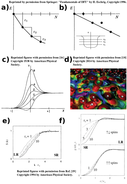
Figure 1: Long-range (left) and short-range (right) theories of electronic structure. (a) and (b) show free energy vs. electron number for a potential well.¹⁵ (c) shows ‘Epstein’ profile of dielectric response^{16; 17} at a metal/vacuum interface. Numbers for each curve give the surface/bulk conductivity ratio. (d) shows surfaces of constant voltage at a water/vacuum interface,¹⁸ (e) and (f) show the correlation function of jellium from accurate calculations.¹⁹

Between the lines of the history above, we find Bose’s famous 1924 Z. Physik paper describing the statistics of bosons, which Einstein noted ‘also yields the quantum theory of the ideal gas,’ and the Thomas-Fermi theory of 1927-28 for a gas of electrons under a fixed applied voltage. Their basic conception was to model the 6-dimensional space of particle locations, $r$ and momenta, $p$ with the volume element,

$$g(p^{\prime})dp^{\prime} =dp^{\prime}\int\delta(|p|-p^{\prime})h^{-3}\,dr^{3}\,dp^{3}$$

$$=4\pi Vh^{-3}p^{\prime 2}dp^{\prime}$$ (1)

Using $p^{\prime}=h\nu/c$ for photons of frequency $\nu$ provides $g(\nu)$, the number of available states for photons near frequency $\nu$. Applying Bose counting statistics to $n(\nu)$ photons occupying $2g(\nu)$ possible states for each frequency gives Bose’s derivation of Planck’s law. In the Thomas-Fermi (TF) model, $p^{\prime}$ is electron momentum. Applying Fermi statistics to the occupancy number $N=2\int^{\hbar k_{F}}_{0}g(k\hbar)d(k\hbar)$ now gives a Fermi distribution for an ideal gas of electrons under a constant external potential (electrostatic voltage). In both cases the number of states is doubled – counting 2 polarizations for photons or 2 spin states for electrons. The result of the first procedure is a free energy expression for the vacuum. The result of the second is a free energy for electrons under a constant voltage.

This idea of a gas with uniform properties uses a long-range field to guess at local structure. Quantitatively, if the voltage at point $r$ is $\phi(r)$, then the theory predicts electrons will fill states up to maximum momentum of $k_{F}=\sqrt{2m_{e}e_{0}\phi(r)}/\hbar$, (where the kinetic energy is $E_{F}=\hbar^{2}k_{F}^{2}/2m_{e}$ and $e_{0}$ is the electron charge) so the local density is,

$$n(r)=k_{F}^{3}/3\pi^{2}.$$ (2)

The resulting model is then usually found to predict long-range properties of metals relatively well. Fig. 1a and b show plots of free energy vs number of electrons in an independent electron solution of the Schrödinger equation for a well of positive potential.¹⁵ Panel b shows a simple adaptation of that model where electrons bind in pairs. The states of the electrons in these exact solutions still represent momentum levels, and are thus qualitatively very close to those of the Thomas-Fermi theory.

The free electron gas evolved into the famous ‘jellium’ model of electron motion rather quickly, as can be seen by the earliest references in a discussion of that model from the late 20th Century.²⁰ The term jellium was coined by Conyers Herring in 1952 to describe the model of a metal used by Ewald²¹ and others consisting of a uniform background density of positive charge. The electrons are therefore free to move about in gas-like motion. At high density, the electrons actually do act like a free gas, so it was possible to use the Thomas-Fermi theory to qualitatively describe the electronic contribution to specific heat, $C_{v}=\pi^{2}k_{B}^{2}T/2E_{F}$, as well as the spin susceptibility and width of the conduction band (after re-scaling the electron mass).²² These are long-range properties arising from the collective motion of many electrons. The predictions become poor for semi-metals and transition metals. It also rather poorly described the cohesive energy of the metal itself. Those cases fail because of the importance of short-range interactions that a free electron theory just doesn’t have.²³

The contrast becomes important at interfaces, as is visible when comparing Fig. 1c,d. On the left is an early model of local charge density response due to placing an external voltage at a point near a metal surface. On the right is a map of the local voltage for one surface configuration of an electrolyte solution computed using an accurate quantum density functional theory. Chloride ions are green, and sodium ions are blue. Treating one of the sodium ions as a test charge, the material response comes from rearrangement of waters (red and white spheres) and Cl^- ions within a nuanced voltage field (colored surfaces).

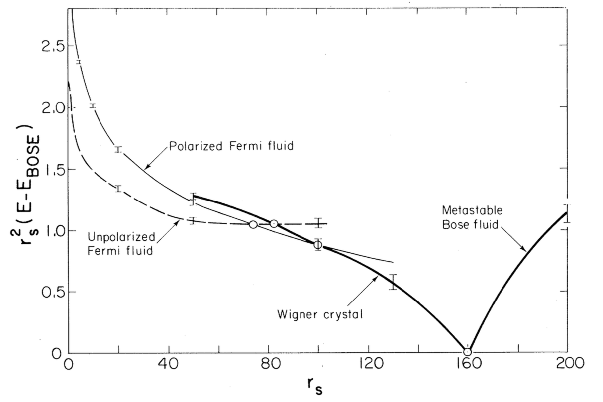
(a) Ground state energy vs. density for the uniform electron gas.²⁶ Four separate phases were observed (at zero temperature). Note that the density axis is reversed by the transformation $1/n=4\pi r_{s}^{3}/3$. Reprinted figure with permission from Ref. 26. Copyright 1980 by the American Physical Society.

(b) Phase diagram of a z:z electrolyte like NaCl where $n$ is the cation concentration. Lines show the position of the spinodal using methods appropriate for each theory, and the minimum indicates a critical point for fluctuation in ionic concentration. Note the temperature axis is reversed by $\beta=z^{2}/dk_{B}T$ and $\eta=\pi nd^{3}/6$, $d$ is the ion diameter. Reprinted from Ref. 35, with the permission of AIP publishing.

Figure 2: Comparing phase diagrams of the electron gas dissolved ions. Both show an insulating phase at low density (labeled Wigner crystal in (a)) and a conducting phase at high density separated by a minimum. The corresponding transition in an electron gas has not been well studied, but critical temperatures feature in the phase diagram of superconducting cuprates (where $n$ is percent of solid impurities).³⁶

It turns out that the electron gas in ‘real’ jellium behaves rather differently at low and high density. At low density, the electron positions are dominated by pairwise repulsion, and organize themselves into a lattice (of plane waves) with low conductivity.²⁴ This low-density state is named the ‘Wigner lattice’ after E. P. Wigner, who computed energetics of an electron distribution based on the lattice symmetry of its host metal.²⁵ At higher densities, collective motions of electrons screen out the pairwise repulsion at long range. This gives rise to a nearly ‘free,’ continuous distribution of electrons with higher conductivity more like we would picture for a metal. Fig. 2(a), from a well-known particle-based simulation of Ceperly and Alder,²⁶ shows the Wigner lattice as well as both spin-polarized and unpolarized high-density states.

Taking the opposing side, early applications of self-consistent field (Hartree-Fock or HF) theory to molecules and oxides noticed that the long-range, collective ‘correlated’ behavior of the electrons was usually irrelevant to the short-range structure of electronic orbitals. Getting the short-range orbital structures right allowed HF theory to do well describing the shapes of molecules and the cohesive energy of metal oxides,²⁷ as well as magnetic properties.²⁸ More recent work has shown explicitly that a model that altogether omits the long-range tail of the $1/r$ potential still allows accurate calculations of the lattice energy of salt crystals.²⁹

Although both theories worked well for their respective problems, the transition from insulating to conducting metals (as electron density increases) also proved to be difficult because it involved a cross-over between both short- and long-range effects. Because of this mixture of size scales required, relying exclusively on a theory appropriate for either short- or long-range produces results that increasingly depend on cancellation of errors. This sort of error cancellation is illustrated by the phenomenology of ‘overdelocalization.’

Well known to density functional theorists, ‘overdelocalization’ is the tendency of continuum models for electron densities (having their roots in the long-range TF theory) to spread electrons out too far away from the nucleus of atoms. The result is that electron clouds appear ‘softer’ in these theories, and polarization of the charge cloud by the charge density of a far molecules contributes too much energy. On the other hand, induced-dipole induced-dipole dispersion forces are not modeled by simple density functionals, and so their stabilizing effect is not present. It has been found that the over-delocalization can be fixed by making a physical distinction between short and long-range forces. However, the resulting binding energies are not strong enough. After the correction, they need a separate addition of a dispersion energy to bring them back into agreement with more accurate calculations.³⁰ Thus, a bit of sloppiness on modeling short-range structure can compensate for the missing, collective long-range effects.

Hybrid Theories in Electronic Structure

When looking at properties like the cross-over between conducting and insulating behavior of electrons, it’s not surprising that successful theories strike a balance between short-range, discrete structure and long-range continuum effects. Even in the venerable Born-Oppenheimer approximation from 1927, we see that atomic nucleii are treated as atoms (immovable point charges), while electrons are described using the wave theory. The separation in time-scales of their motion makes this work. By the time the atoms in a molecule have even slightly moved, the electrons have zipped back and forth between them many times over.

Correlation functions are a central physical concept in the debate between long and short range ideas. The distance-dependent correlation function, $g(r)$, measures the relative likelihood of finding an electron at the point, $r$, given that one sits at the origin. One of the first attempts at accounting for electron-electron interaction was to use perturbation theory to add electron interactions back into the uniform gas model ($g(r)=1$). The first order perturbation modifies this by looking at interactions between electrons of the same spin. This interaction is termed the exchange energy, since it comes from pairs of electrons with the same spin exchanging momentum.²² After the correction, electrons with parallel spin now have smaller density at contact, $g(r)=1-\tfrac{9}{2}(\sin(k_{F}r)-k_{F}r\cos(k_{F}r))^{2}/(k_{F}r)^{6}$.

The correlation function between infinite periodic structures is, $S(k)$, the long-range analogue of $g(r)$ (in fact its Fourier transform). The function $S(k)$ is called the structure factor by crystallographers. If the system consisted only of electrons, the structure factor could be measured directly by light or electron scattering experiments. There, $S(k)$ is the intensity scattered out at angle $\theta=2\arcsin(\lambda k/4\pi)$ when the material is placed into a weak beam of photons or electrons of wavelength $\lambda$ pointed in the $\theta=0$ direction. This function has been computed using an accurate particle simulation technique and shown in Fig. 1e,f.¹⁹ The curves are labeled by $r_{s}=(3/4\pi n)^{1/3}$, measured in units of Bohr radii.

There is a duality between short and long range perspectives inherent in $g(r)$ and $S(k)$ as well. Long-range behavior appears at large $r$ when $g(r)$ approaches 1. At small $r$, the geometry of inter-particle interactions determines the shape of $g(r)$. Because particle dynamics is carried out in real-space, $g(r)$ tends to be used by its practitioners to characterize short and long-range structure. Analytical solutions of many models, and especially those aiding experimental measurements, are simpler in Fourier space. There, $S(0)$ is the integral of $g(r)$. It provides information on the total fluctuations in the number of particles, and is a long-range quantity from which the compressibility, partial molar volumes, and other properties can be computed.³¹ Short-range structures that repeat with length $d$ show up as peaks in $S(k)$ at correspondingly large $k=2\pi/d$.

Back to the metallic/insulator problem, between 1950 and 1953 Bohm and Pines pioneered the idea of explicitly splitting the energy function (Hamiltonian) governing electron motion into local and long-range degrees of freedom.^{32; 33; 34} Using the intuition that long-range collective motions of electrons should look like the continuous plane-wave solutions to Maxwell’s theory, they added and subtracted those terms and called them ‘plasmons.’ (Fig. 4d) Just like photons, the plasmons are continuous waves when treated classically, but are quantized particles when understood quantum mechanically.

What remained after the subtraction was a Hamiltonian whose interactions were only short-ranged, but could not be treated with a continuum description. Instead, the short-range part describes interactions between effective discrete particles which Bohm and Pines dubbed ‘quasiparticles.’ The quasiparticles were like packs of electrons surrounded by empty space, ‘holes.’ The quasiparticles thus have larger mass and softer, screened, pair interactions (explaining why the mass has to be fixed when applying the free electron theory to metals). These new ‘renormalized’ electron quasiparticles could even have effective pairwise attraction. This latter effect was a central component to the BCS model of superconductivity, where the quasiparticles are known as ‘Cooper pairs.’ Because of its dual representation, the Bohm-Pines model gave good answers for both cohesive energies and conductivities – and described the cross-over between insulating and metallic regimes as electron density is increased.²⁴

For all its descriptive power, the Bohm-Pines approach was often lamented for its requirement for a specific set of approximations. Most damningly, it required inventing a continuum of plasmons to describe the long-range interactions of a finite set of electrons. This adds infinite degrees of freedom to a system with an initially finite number. It also required the plasmons to stop and the particles to commence at some cutoff wavelength. These troubles lead us into the problem of renormalization group theory, which is beyond the scope of the present article.

In fact, in 1954, just after the publication of the last article in the Bohm and Pines series above, Lindhard provided a model for collective electronic response of a metal that involved only the metal’s correlation function (by means of its dielectric coefficient, $\epsilon$).³⁴ Following a decade later in 1964-65 was Hohenberg, Kohn and Sham’s density functional theory.^{37; 38; 39} Both developments rephrased the description of electronic structure in terms of a continuous field of electron density. Linear response (perturbation) theory says that an initially homogeneous density $n_{0}$ responds to an applied field, $\phi$ as,

$$\Delta n(r)=n_{0}\int\chi(r,r^{\prime})\phi(r^{\prime}),$$ (3)

where $\chi(r,r^{\prime})$ is the Fourier transform of the structure factor above. Their defining characteristic is the focus on continuous response of that density to a continuous external field, $\rho(r)=\rho[\phi(r^{\prime})](r)$.

The theory may be understood as a fully long-ranged point of view that includes short-range effects indirectly through $S(k)$. It shows how to use integration to calculate all thermodynamic quantities from structure factor. The only problem is that it does not broach the issue of how to predict the structure factor. One well-known method is to assume the probability of $n(r)$ is a Gaussian on function space (so the exponent depends on $\int n(k)^{2}/\chi(k)\,dk^{3}$, and $\chi(k)$ is just slightly different from $S(k)$). In that case, the inverse of the correlation function ($1/\chi(k)$) is a self-energy term plus the inter-particle energy function. This assumption is known as the random phase approximation (RPA), named because of its historical discovery by Bohm and Pines following from neglecting couplings between a set of linearly independent (Fourier) modes, $n(k)$. This ends up excluding all non-Gaussian fluctuations.

The ‘dielectric’ ideas encapsulated in the linear response theory of Eq. 3 can be combined with the free electron model of Eq. 2 ($T[n]$ proportional to $n^{5/3}$), or a wavefunction calculation of the kinetic energy, $T[n]$, to synthesize modern density functional theory (DFT).^{40; 20} It writes the electron configuration energy as,

$$A[\phi]=\inf_{n(r)}T[n]+E_{\text{XC}}[n]+\int n(r)\left(\phi(r)+\frac{1}{2}\int dr^{\prime 3}\frac{n(r^{\prime})}{4\pi\epsilon_{0}|r-r^{\prime}|}\right)\,dr^{3}.$$ (4)

Now the (long-range) correlation function of the electron, $\chi$, is obtained from the curvature of $A[\phi]$. Mathematically, the unknown structure factor has been migrated into an unknown functional, $E_{\text{XC}}[n]$. The initials stand for exchange and correlation, its two major components. The principle advantage gained by this rephrasing is that new, accurately known (usually short-range) terms like $T[n]$ can be added to $A[\phi]$ in order to decrease the burden on $E_{\text{XC}}$ to model ‘everything else.’ The disconnect between short and long-range energies can be shoveled into some fitting parameters.

Again moving forward 40 years, the relative unimportance of long-range Coulomb interactions for local structuring noticed by Lang and Perdew^{41; 29} lead to the suggestion that the density functional method itself should also distinguish between short and long range structural effects. Implementation of this idea was perhaps first carried out by Toulouse, Colonna and Savin in 2004.⁴² There, the local density approximation deriving its roots in the TF theory is applied to describe short-range interactions, while the HF theory is used to ensure proper electron-pair repulsion (exchange) energies at long-range. The association of HF with long-range and density functional (DF) with short-range apparently runs counter to our association between continuum, density-based, models for long-range interactions vs. discrete, particle-based models for short-range interactions. A major complication with our association is that it is known that the HF method describes the long-range (asymptotic) electronic interactions well, whereas the DF method does not. DF methods were historically used to describe the ‘entire’ energy function, and have thus been tailored to describe quasi-particles (the so-called exchange hole), rather than asymptotics. This association was put to the test shortly after by Vydrov and co.⁴³ using an earlier DF called LSDA that is not strongly tailored in this way. They separately averaged the short- and long-range components of HF and DF and checked their ability to predict the cohesive, formation energies of small molecules. Doing so, they discovered that models with no HF at long range had similar descriptive power to those that used only DF at short range and only HF at long range. Split-range functionals are still an evolving research topic.

Liquid-State Theories

The divide between short and long-range, discrete, and continuous distributions also plays a key role in the development of thermodynamic theories for gasses and liquids. In the 1860s, Boltzmann proposed his transport equation for the motion of gas density over space and time. The model employed the famous stoßzahlansatz, which states that the initial positions of molecules before each collision is chosen ‘at random.’ (Fig. 4a) In the original theory, the probability distribution over such random positions was often confused with their statistical averages⁴⁴ – a point which lead to enormous confusion and controversy persisting even until 1960.⁴⁵

This history very nearly parallels the development of electronic density theories. After electromagnetism and gas dynamics had been worked out at the end of the 19th century, Gibbs’ treatise on statistical mechanics laid out the classical foundations of the relationship between statistics and dynamics of molecular systems. Nevertheless, there were contemporary arguments with Ehrenfest and others about the need for introducing statistical hypotheses into an exact dynamical theory.² Early on, it had been hoped that an exact study of the motion of the molecules themselves could predict the appropriate ‘statistical ensemble’ by finding long-time limiting distributions. However, that hope was spoiled by the notice that initial conditions must be described statistically. The idea persists even at present, though it has been tempered by the recognition that sustaining nonequilibrium situations requires an infinitely extended environment, which has to be represented in an essentially statistical way.⁴⁶

The resolution, according to Jaynes,⁴ is to understand the Boltzmann transport equation as governing the 1-particle probability distribution, $NP(r|C)$, rather than the average amount of mass, $n(r)$, at point $r$. It turns out that this switch in perspective from exact knowledge of all particle positions to probability distributions is one of the key ways of separating short and long-range effects. Two of the oldest and most widely known uses of this method are in the dielectric continuum theory dating from before Maxwell’s 1870 treatise, even to Sommerfeld (Fig. 4c), and the Debye model of ionic screening from 1923. For both, a spatial field $E(r-r_{0})$, emanating from a discrete molecule at $r_{0}$, is put to a bulk thermodynamic system whose average properties are well-defined using, for example, $P(r|E)$ for the dipole density $\mu(r)$ at point $r$, due to a field, $E$ or $n(r;\phi)$ for the ion density at point $r$ due to a voltage, $\phi$. Treating $\phi$ and $E$ as weak perturbations and looping $\mu(r)$ (or $n(r)$) back in as additional sources gives a self-consistent equation for the response of a continuum.

As was the case for electronic structure theory, the most concise description of this type of self-consistent loop is provided by a density functional equation for the Helmholtz free energy (with $\beta=1/k_{B}T$),

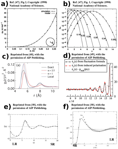
Figure 3: Short- and long-range theories of solvent dipole and electrolyte structure. (a) and (b) show free energies and number occupancy distribution for spherical cavities in water.⁴⁷ (c) shows the dielectric response in a spherical geometry⁴⁸ and (d) shows the dielectric permittivity computed in a slab geometry.⁴⁹ (e) and (f) show the correlation function of a supercritical Lennard-Jones fluid near $n=0.52/\sigma^{3}$, $T=1.34\epsilon/k_{B}$.⁵⁰

$$\beta A[E,\beta] =\inf_{\mu\in\{\mu\}}\left[-\log(g[\mu])-\beta E\cdot\mu\right]$$

$$\approx-\ln\sum_{\mu\in\{\mu\}}g(\mu)e^{\beta E\cdot\mu}.$$ (5)

The curvature of $A$ with changing applied field, $E$, gives the response function which is related to the conventional dielectric. Consider first a case where $\mu$ contains enough information to exactly assign a dipole to every one of $N$ molecules. An example would be a single molecule with twice as many ways to create a small dipole as a large one, $g(4\text{ D})=2$ and $g(2\text{ D})=4$ (1D = 1 Debye). Then $g(\mu)$ is a product over counting factors. The free energy, $A$, will have jump discontinuities in its slope as the field, $E$ is varied because the solution jumps from one assignment ($\mu=2$ D) to another ($\mu=4$ D at $\beta E\geq(\ln 2)/(2\text{ D})$). Its graph is very much like Fig. 1a. In a discrete function space, density functional theory equations yield solutions exhibiting the a discrete nature.

On the other hand, if $g(\mu)$ varies continuously with $\mu$ in some range of allowed average densities, then the solution will describe a smooth field free energy. Interestingly, starting from the first situation and computing

$$S[\bar{\mu},\beta]=-\beta\sup_{E}\left[A[E,\beta]+\int E(r)\cdot\bar{\mu}(r)dr\right],$$ (6)

leads to such a continuous version of $\log g(\mu)\approx S(\mu)$ (in fact its concave hull). This concave function allows densities that are intermediate between discrete possibilities for the system’s state. Such intermediate densities could only be reached physically by averaging, so that $\bar{\mu}$ is an average polarization over possible absolute assignments of dipoles to molecules, $\mu$.

After the theory of self-consistent response to a long-range field had been worked out, further development of liquid-state theory had to wait 40 years for developments in quantum-mechanical interpretation of light absorption and scattering experiments. Some early history is given in Ref. 51 and Debye’s 1936 lecture⁵² in which he explains how electronic and dipole orientational polarization could be clearly distinguished from measurements of the dielectric capacitance of gasses along with the great advancements made in the 1920s (which Debye credits to von Lau in 1912) of using x-ray and electron scattering to confirm molecular structures already adduced by chemists from symmetry and chemical formulas alone. Thus, the long-range theory gave a comprehensive enough description of macroscopic electrical and density response that it could be used as a basis to experimentally determine local structure.

With statistical mechanics, quantum mechanics, and molecular structure in hand, liquid-state theories developed in the 1930s-50s through testing hypotheses about the partition function against experimental results for heat capacities. One of the earliest models was the ‘free volume’ (also known as cell model) theory, developed by Eyring and colleagues and independently by Lennard-Jones and Devonshire in 1937. The theory was put on a statistical mechanical basis by Kirkwood in 1950,⁵³ as essentially expressing the free energy of a fluid in terms of the free energy of a solid composed of freely moving molecules trapped, one each, in cages exactly the size of the molecular volume, plus the free energy cost for trapping all the molecules in those cages in the first place. It competed⁵⁴ with the ‘significant structure’ theory of liquids (also proffered by Eyring and colleagues^{55; 56}). In the significant structure theory (Fig. 4f), the partition function for the fluid is described as an average of gas-like and solid-like partition functions to account for the difference in properties between highly ordered and more disordered regions (which contain vacancies).

Scaled Particle vs Integral Equations

Also around that time, a competition emerged between the scaled particle theory⁵⁷ and the ‘integral equation’ approach based on (and now lumped together with) Percus and Yevick’s^{58; 59} closure of a theory created by Ornstein and Zernike in 1914 to calculate the effect of correlated density fluctuations on the intensity of light scattered by critically opalescent fluids.⁶⁰ This connection was significant, since theories of the correlation function prior to 1958 applied the superposition approximation due to Kirkwood, Yvon, Born, and Green (ca. 1935).^{61; 62}

The scaled particle theory (SPT) approach takes the viewpoint that the number, sizes and shapes of molecules in a fluid are determined by integrating the work of ‘growing’ a new solute particle in the middle of a fluid. Its organizing idea is that the chemical potential of a hydrophobic solute is equal to the work of forming a nanobubble in solvent. For simple hard spheres, the work is $PdV$, where $P=k_{B}Tn_{0}G(d)$, $n_{0}$ is the bulk solvent density, and $G(d)$ (Fig. 4b), the density of solvent molecules on the surface of the solute of diameter $d$. Hence, knowing the contact density for any shape of solute molecule provides complete information on the chemical potentials of those molecules. This very local idea can be related to counting principles at very small sizes,⁶³ and continued through to macroscopic ideas about surface tension at very large sizes – creating a way to interpolate between the two scales.

On the other hand, the integral equation approach expresses the idea that long-range fluctuations in density are well described by a multivariate Gaussian distribution. If the probability distribution of the density, $n(r)$, was actually Gaussian, its probability would be,⁶⁴

$$P[n(r)]=P[n_{0}]\exp\left(-\frac{\beta}{2}\iint drdr^{\prime}\,(n(r)-n_{0})G(r,r^{\prime})(n(r^{\prime})-n_{0})\right)/Z[\beta G],$$ (7)

where $G(r,r^{\prime})\equiv\mathrm{const}\cdot\delta(r-r^{\prime})-c(r-r^{\prime})/\beta$. In the RPA, $-c(r)/\beta$ is energy for placing a pair of molecules at positions $r$ and $r^{\prime}$.⁶⁵

When they are not Gaussian distributed, the correlations in instantaneous densities, $n(r)$, provide a means of estimating $c$, the direct correlation function.⁶⁶ This long-range idea has been used to show that $G$ degenerates to the pairwise energy for very large separations ($G(r)\to U(r)$ as $r\to\infty$). For simple hard spheres, it can also be related to counting principles at short separations, since there the correlations must drop to -1, expressing perfect exclusion. Assuming limits both hold right up to the discrete boundary of a solute yields the mean spherical approximation (MSA, Fig. 4b).

These two theories thus express, in pure form, the divide between short-range and long-range viewpoints on molecular structure. Integral equation theories are most correct for describing continuum densities and smooth interactions. Theories that, like SPT, are based on occupancy probabilities of particles in well-defined local structures and geometries are most correct for describing short-range interactions that can contain large energies and discontinuous jumps.

Fig. 3b shows $P(n|d)$, the probability that a randomly chosen sphere of radius $d$ contains exactly $n$ discrete water molecules. Each curve is marked by its value of $d$ in nanometers. The free energy for creating an empty nanobubble of size $d$ in water is shown in its counterpart, Fig. 3a. Both computations are very closely related, and easiest to do from the local picture of scaled particle theory. The cavity formation free energy (Fig. 3a) is, in principle, also able to be computed from a density functional based on relating the logarithm of Eq. 7 with the entropy.⁶⁴ However, when the calculation is done in the usual density functional way the cavity formation free energy is surprisingly difficult to reproduce.^{67; 68} This difficulty is related to the abrupt decrease in solvent density to zero at the cavity surface. In addition to mathematical difficulties,⁶⁹ this complicates creating a physically consistent functional from bulk properties alone. From scaled particle theory, we know the free energy should scale with the logarithm of the volume for small cavities, but later switch over to scale with the surface area. The transition distance is determined by the size of discrete solvent molecules.

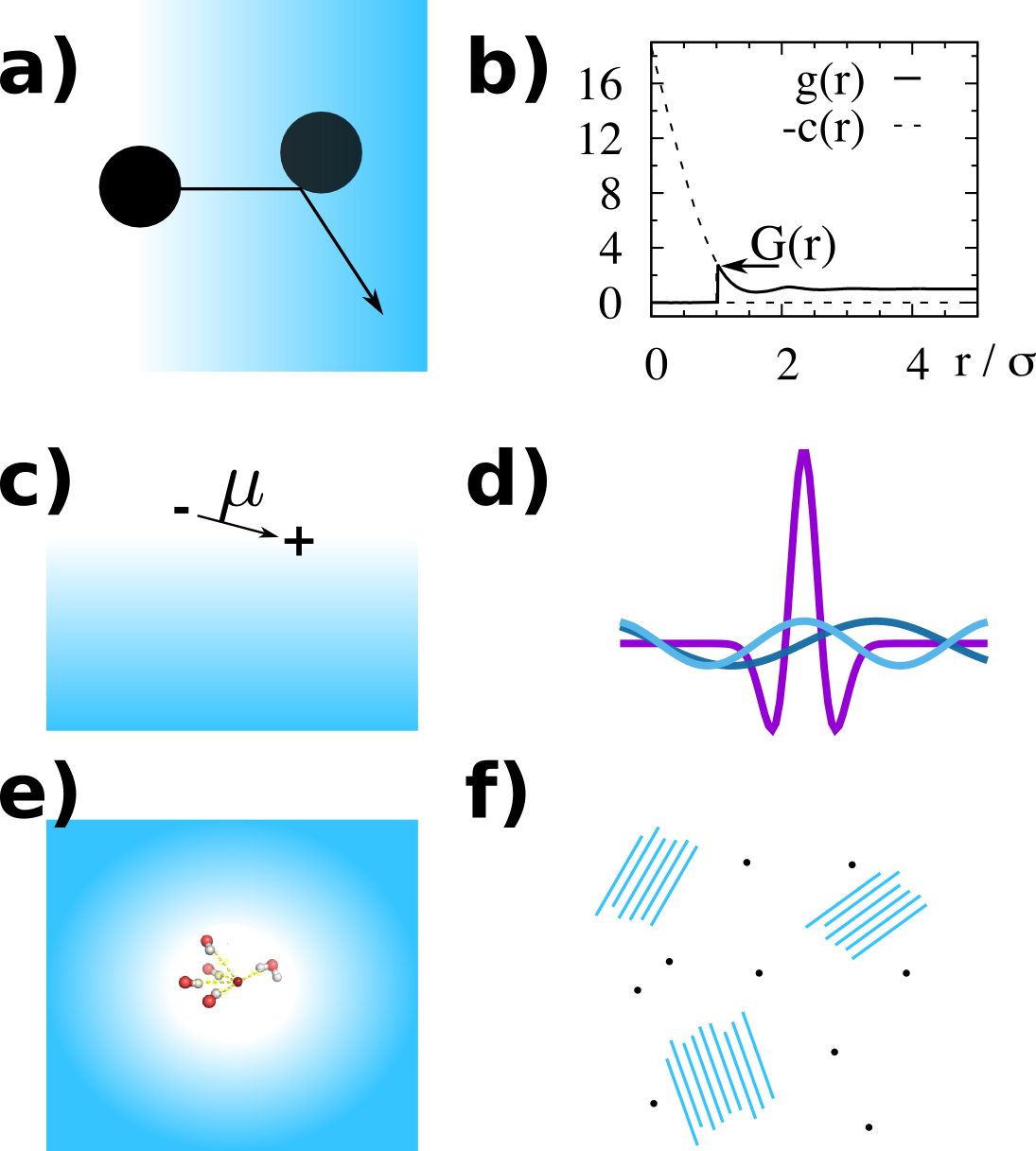
Figure 4: Hybrid discrete/continuum theories. (a) Boltzmann picture of scattering by one particle chosen ‘at random’ from the continuum. (b) Mean spherical approximation for the hard sphere fluid of diameter $\sigma$. $g(r)$ and $c(r)$ are known at $r<<\sigma$ and $r>>\sigma$, but the central region is a guess. (c) Sommerfield conception of a dipole above a continuous polarizable medium. (d) Bohm-Pines conception of a quasiparticle (purple, central peak) and two long-range plasmons (blue). (e) Dressed ion, quasichemical, or Lorenz-Lorentz-Mossotti-Clausius⁵¹ cavity models of a discrete molecule in a continuum solvent, (f) significant / inherent structure theory of a coexisting mixture of ordered and disordered regions making up an overall homogeneous phase.

Perturbation Theories

Slowly but surely during the same time period as integral equation theories were being developed the method of molecular dynamics emerged.⁷⁰ Its primary limitations of small, fixed, particle numbers, large numbers of parameters, finite sizes and short timescale simulations weigh heavy on the minds of its practitioners.⁷¹ Early models of water needed several iterations before reproducing densities, vaporization enthalpies and radial distribution functions from experiment. Initial radial distributions from experiment were wrong, and the models had to be corrected and then un-corrected to chase after them.⁷² Surprisingly, early calculations took the time and effort to calculate scattering functions and frequency-dependent dielectrics to compare to experiment.^{73; 74; 75} By contrast, the bulk of ‘modern’ simulations report only the data that can be readily calculated without building new software.

By checking data from integral equations against molecular dynamics (MD) and scattering experiments it was clear by 1976 that many powerful and predictive methods had been created to describe the theory of liquids.^{76; 77} Nevertheless, there remained even then lingering questions about the applicability of integral methods to fluids where molecules contained dipole moments, and the treatment of long-range electrostatics in MD. Some difficulties in modeling phase transitions and interfaces were anticipated, but it was hardly expected that bulk molecular dynamics methods themselves would stall and eventually break down when simulating liquid/vapor and liquid/solid surfaces.

This trouble is illustrated by the simulation community’s reception of the work leading to Fig. 3c,b. Both show the dielectric response function for water dipoles at the interface with a large spherical particle (left) or vacuum (right). The latter shows a correlation function computed from all-atom molecular dynamics by Ballenegger.⁴⁹ This full computation was preceded two years earlier by less well-cited theoretical work from the same author.⁷⁸ As of writing, the citations counts are 140 and 19, respectively. Even after its publication, the technical difficulties caused by simulating collective dipole correlations inside a finite size box cast a cloud over the interpretation that drove Ballenegger back into those fine details for the following nine years.^{79; 80} On the left (Fig. 3c) is a simulation of water’s dipolar response next to a large sphere.⁴⁸ The finite-size effects are less severe, and a comparison (not common in contemporary literature) is made to analytical theories that apply to infinite systems. However, those analytical theories work best at long-range, and disagree on the short-range order. The disagreement is jarring because energetic contributions of long and short-range order are on the same order of magnitude.

It was also beginning to be recognized that there were two complementary approaches to the theory of fluid structure. The short-range viewpoint stated that the radial distribution function should be reproduced well at small intermolecular separations (small distance in real-space as in Fig. 3f). This leads to good agreement with interaction energies and pressures so that the virial and energy routes to the equation of state work well.⁵⁰ The long-range viewpoint instead emphasizes reproducing the structure factor at small wavevectors (as in Fig. 3e). Because of this, it favors using the compressibility route to the equation of state and leads to good agreement with fluctuation quantities.⁸¹

Inherent structures

Water proved to be a major challenge to molecular models because of its mixture of short-range hydrogen bonding and long-range dipole order.⁸² One successful physical picture of water was provided by the Stillinger-Weber ‘inherent structure’ model introduced in the early 1980s.⁸³ It represented a cross between the ‘significant structure’ theory and the free volume theory. In it, molecules are fixed to volumes defined by their energetic basins, rather than by a rigid crystal lattice. Where the free volume theory had only one reference structure, the inherent structure (like the significant structure theory) had many. One for each basin. Each energetic basin looks, on an intermediate scale, like a distortion of one of the crystalline phases of ice. Thermodynamic quantities can be predicted using the energies and entropies associated to each basin – by virtue of the minimum energy structure and the number of thermal configurations mapping to that minimum.

Hybrid Theories in Liquid-State Structure

The Lennard-Jones fluid presented a challenge to the integral equation and scaled particle theories above because it contains both short-range repulsion and long-range attraction. At high densities, however, it was found that the radial distribution function was almost identical to the radial distribution for hard spheres (compare Fig. 3e and Fig. 4b). The transition from liquid to solid was also described fairly well using the hard-sphere model. On the other hand, at low densities the distribution function could be described by perturbation from the ideal gas. These two discoveries justify the use of a perturbation theory to calculate the effect of long-range interactions at very low and very high densities.⁸⁴ A comparison of molecular dynamics with integral equation plus correction theories is shown in Figs. 3e,f.⁵⁰

At intermediate densities, however, a liquid-to-gas phase transition occurs that can be qualitatively understood, but not explained well as a perturbation from either limit. Instead, the integral equation method turns out to hold the best answer in the supercritical region.⁸⁵ It is often encountered in the form of a perturbation theory from the critical point.⁸⁶ It is no accident that the integral equation method works well here. Supercritical fluids are characterized by long-range correlations that can take maximum advantage of that theory. For the same reason, integral equations describe the compressibility well, but do poorly on the intermolecular energy.

Comparing to developments in electronic structure raises the question of whether perturbation theory could fix the short-range correlations in high and low density fluids. This approach was popularized by Widom’s potential distribution theory.⁸⁷ Its central idea is to drop a spherical void into a continuum of solvent, and then to drop a solute into its center. This divides the new molecule’s chemical potential into a structural part (due to cavity formation) and a long-range part (due to response of solvent to the molecule). Originally, the former were based on a local density approximation from the hard sphere fluid and the latter from a pairwise term that amounted to a van der Waals theory.

Around 1999, this basic idea had been combined with older notions about working with clusters of molecules to create a new ‘quasi-chemical’ theory.⁸⁸ It refined the simple process of creating an empty sphere devoid of solvent into that of creating a locally well-defined cluster of solvent molecules. The free energy required for this process is still local and structural, but now the entire cluster of solute plus solvent can be regarded as one, local, chemical entity. In order to work with molecules that have ‘loose’ solvent clusters, a third step was also added. After pulling solvent molecules into a local structure and adding the long-range interactions between solute and solvent, the third step releases the solvent cluster, liberating any energy that might have been trapped by freezing them.⁸⁹

The opposite of this short-range-first approach could be an inverse perturbation theory – first deciding on the long-range shape of correlation functions and second correcting them for packing interactions at short-range. This kind of correction would look like an adjustment to the solution of the Poisson-Boltzmann equation. Such an approach may first have been presented in Refs. 90; 91, and followed with interesting modifications of the Debye theory.^{92; 93; 94} Even more recently, the basic idea was rigorously applied to molecular simulation models by Remsing and Weeks. Their scheme eliminates a hard step between short and long-range in the first step by splitting the Coulomb pair potential into smooth, long-range and sharp, short-range parts. The long-range forces (from the smooth part of the potential) are used to compute a ‘starting’ density using RPA-like perturbation from a uniform fluid. Although it seems a lot like the molecular density functional method,^{95; 96; 62} the density after the first step remains smooth at the origin, lacking any hard edges. It has previously been considered under the title ‘ultrasoft restricted primitive model.’⁹⁷ Remsing and Weeks added a final step to this model to create a cavity at the origin and compared the results to MD simulations.

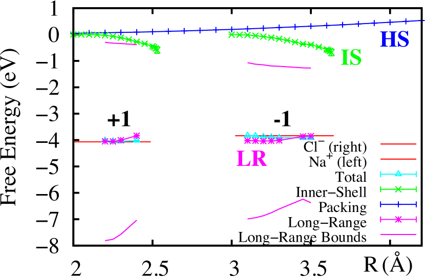
(a) Ion solvation free energy components for the short-range (empty cavity first) model computed from an MD model of NaCl in SPC/E water. $R$ is the cavity radius, ‘HS’ denotes the cavity formation cost, ‘LR’ is the full ion-SPC/E water interaction after a cavity is present, and ‘IS’ is the free energy of removing the cavity constraint.

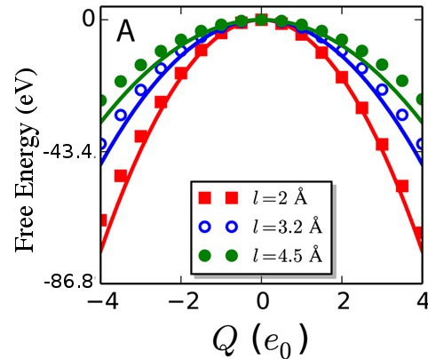
(b) Interaction free energy of SPC/E water with a Gaussian charge distribution, $Q\exp(-r^{2}/l^{2})/(l\sqrt{\pi})^{3}$. Points correspond to simulation data, while lines assume a constant dielectric model. Adapted with permission from Ref. 98, Copyright 2016 American Chemical Society.

Figure 5: Comparing components of the SR-first (left) and LR-first (right) calculations of the free energy gained on dissolving a charged ionic species in water.

Detailed molecular simulations have been used to compare the two approaches with exact simulations by brute force calculation of all the energetic contributions. Focusing on the short-range structure leads to a model whose first step is to form an empty cavity in solution (blue curve in Fig. 5(a), labeled ‘Packing’). Fig. 5(a) shows the free energies of the next step (Na⁺ and Cl^- ions) divided into ‘long-range’ and ‘inner-shell’ parts of the re-structuring.⁹⁹ All points come from MD. If, instead, the long-range interaction between an ion and solvent occurs first, we are lead to couple the solvent to the smooth electric field of a Gaussian charge distribution. Fig. 5(b) shows the free energy of that first step as a function of charge for a variety of Gaussian (smoothing) widths. The lines show continuum predictions, and the points show MD.

Integral equation approaches to the dipolar solvation process have also continued independently. Matyushov developed a model for predicting the barrier to charge transfer reactions.¹⁰⁰ In that work, the dipole density response function to the electric field of a dipole is worked out in linear approximation. A sharp cutoff is used to set the field to zero inside the solute, resulting in a hybrid short/long range theory. The approach succeeds because the linear response approximation (stating density changes are proportional to applied field) is correct at long range, where the largest contributions to the solvation energy of a dipole originate. Other authors have expanded on numerical and practical aspects of correlation functions.^{101; 102; 103}

The theme of separating long-range, continuous vs. short-range, discrete interactions runs throughout numerous other molecular-scale models. Models in this category include the ‘dressed’ ion theory, which posits that ions in solution always go in clad with strongly bound, first shell, water molecules so that their radius is larger than would be suggested from a perfect crystal (Fig. 4e). These enlarged radii appear in the Stokes-Einstein equation to describe the effect of molecular shape on continuous water velocity fields when computing the diffusion coefficients for ions.¹⁰⁴ They should also appear to describe how excluded volume of ions will affect the continuous charge distribution predicted by the primitive model of electrolytes. This modification is not common, and so would yield some nonstandard plots of hydration free energy as a function of ion concentration.¹⁰⁵ Solvent orientational order changes form again beyond about 1.5 micrometers due to the finite speed of light.¹⁰⁶ The Marcus theory of electron transport describes two separate, localized structural states of a charged molecule that interact with a continuously movable, long-range, Gaussian, field. Larger magnitude fluctuations in the solvent structure lead to broader Gaussians, which in turn are the cause of more frequent arrival at favorable conditions for the electron to jump. It is common practice in quantum calculations to explicitly model all atoms and electrons of a central molecule quantum-mechanically while representing the entirety of the solvent with a continuous dielectric field.^{107; 108; 109}

The theories above are not perfect. They show issues precisely at the point where short- and long-range forces are crossing over. At high ionic concentrations, the dressed ion theory breaks down due to competition between ion-water and ion-ion pairing. When solvent molecules are strongly bound, the use of a continuous density field cannot fully capture their influence on thermodynamic properties. Even without strongly bound solvent, dielectric solvation models leave open the important question of whether electrons from the fully modeled molecule are more or less likely to ‘spill out’ into the surrounding solvent. Returning back to Aristotle’s objection to discrete objects, it is known that density based models don’t accurately capture the free energy of forming a empty cavity.^{67; 68} Thousands of years on, we are still vexed by the question of how to understand the interface between material objects and vacuums.

The Future: A Middle Way

Early Eastern thought tends to place opposing ideas next to one another in an attempt to understand them as parts of a whole picture. Written around the beginning of the Middle ages, in 400 AD, the Lankavatara Sutra relates Buddha’s view that this unity applies to atoms and ‘the elements’ (which refer to something like the classical Greek elements). Taking liberties, we can say he is discussing a process like instantaneous disappearance (annihilation) of a quantum particle in saying, “even when closely examined until atoms are reached, it is [only the destruction of] external forms whereby the elements assume different appearances as short or long; but, in fact, nothing is destroyed in the elemental atoms. What is seen as ceased to exist is the external formation of the elements.” Bohr was well-known for his view on the ‘complementarity’ principle, stating in this context that the act of removing a particle makes its number more definite, while making the amount of energy it exchanged with an external observer undefined.¹¹⁰ Perhaps inspiring to Bohr sixteen centuries later,¹¹¹ the quote concludes, “I am neither for permanency nor for impermanency … there is no rising of the elements, nor their disappearance, nor their continuation, nor their differentiation; there are no such things as the elements primary and secondary; because of discrimination there evolve the dualistic indications of perceived and perceiving; when it is recognised that because of discrimination there is a duality, the discussion concerning the existence and non-existence of the external world ceases because Mind-only is understood.” Bohr’s complementarity could be contrasted with physicist John Wheeler. He advocated, as a working hypothesis, that participants elicit yes/no answers from the universe. Replies come as discrete ‘bits,’ and are ultimately the reason that discrete structures emerge whenever continuum models try to become precise.¹¹² Wheeler, in turn, could be contrasted with Hugh Everett, whose working hypothesis was that the universe operates by pure wave mechanics.^{113; 114} A modern resolution of those debates invokes small random, gravitational forces to explain how quantum particles could become tied to definite locations.¹¹⁵ It is does not appear that there will be a resolution allowing us to do away with either continuum or discrete notions.

Of course, it is impossible to deduce scientific principles if we include any elements of mysticism in a theory. Nevertheless, the debate on the separation between short and long-range seems to permeate history. This idea that a meaningful understanding of collective phenomena should be sought by combining physical models appropriate to atomic and macroscopic length scales was taken up even recently by Laughlin, Pines, and co-workers.³⁶ They state, “The search for the existence and universality of such rules, the proof or disproof of organizing principles appropriate to the mesoscopic domain, is called the middle way.”

On one account it is clearly possible to set the record straight. There are well-known ways of converting local structural theories into macroscopic predictions and as vice-versa. Bayes’ theorem states that, for three pieces of information, $A$, $B$, and $C$,

$$P(A|BC)=\frac{P(B|AC)P(A|C)}{P(B|C)}.$$ (8)

If ‘C’ represents a set of fixed conditions for an experiment, ‘B’ represents the outcome of a measurement, and ‘A’ represents a detailed description of the underlying physical mechanism (for example complete atomic coordinates), then Bayes’ theorem explains how to assign a probability to atomic coordinates for any given measurement, ‘B’. Of course, in a reproducible experiment, $C$ will completely determine $B$, so $B$ = $B(C)$. Thus, the probability distribution over the coordinates is a function only of the experimental conditions, $P(A|BC)=P(A|C)$. This summarizes the process of assigning a local structural theory from exactly reproducible experiments.

On the other hand, a local structural theory provides an obvious method for macroscopic prediction. Given a complete description, ‘A,’ simply follow the laws of motion when interacting with a macroscopic measuring device, ‘B.’ This would properly be expressed in the language above as $P(B|AC)=P(B|A)$, since the experimental conditions are irrelevant. Bayes’ theorem then gives us a conundrum, $P(B|C)=P(B|A)$, stating that every microscopic realization of an experiment must yield an identical macroscopic outcome.

The solution to the puzzle is to realize that unless an experiment is exactly reproducible, $BC$ is always more informative than the conditions, $C$, alone and $P(A|BC)\neq P(A|C)$. This explains why studying exactly integrable dynamical systems is such a thorny issue, and is the central conceptual hurdle passed when transitioning from classical to quantum mechanics. Now identifying ‘B’ with a partial measurement that provides a coarse scale observation of some long-range properties, $P(A|BC)$ describes a distribution over the short-range, atomistic, and discrete degrees of freedom. Because of experimental uncertainty, the exact location of those atoms is evidently subjective and unknowable (since it is based on measurement of $B$). Nevertheless, it can in many cases be known to a high degree of accuracy.

Density functional theory traditionally focuses on $P(B|C)$, where ‘B’ is the average density of particles in a fluid and ‘C’ is the experiment where a bulk material is perturbed by placing an atom at the origin. However, with a minor shift in focus, $P(B|A^{\prime}C)$ can also be found, representing the average density under conditions where a particle is placed at the origin and some atomic information, $A^{\prime}$ is also known. The objective of such a density functional theory would be to more accurately know the long-range structure by including some explicit information on the short-range structure. The dual problem is to predict $P(A|B^{\prime}C)$, the distribution over coordinates when we are provided with some known information on the long-range structure. In a complete generalization, we might focus instead on $P(AB|A^{\prime}B^{\prime}C)$, representing the average density and particle distribution under conditions where density and particle positions are known only in part. Bayes’ theorem shows us that such a generalization would just be the result of weaving the primal and dual problems together, since (given the redundancies, $B^{\prime}=B^{\prime}(B)$ and $A^{\prime}=A^{\prime}(A)$), $P(A|A^{\prime}B^{\prime}C)=P(A|B^{\prime}C)/P(A^{\prime}|B^{\prime}C)$, and $P(B|A^{\prime}B^{\prime}C)=P(B|A^{\prime}C)/P(B^{\prime}|A^{\prime}C)$.

The arguments above can be repeated for each of the elements in Table 1 – replacing SR with $A$ and LR with $B$. What emerges is a persistent pattern of logical controversy, where a problem can be apparently solved entirely from either perspective. In some areas, one of the other approach is more expedient. In every case, however, recognizing and using both sides has proved to be profitable. Comparing these two perspectives, we find that the discussion concerning the existence of long and short-range theories ceases, leaving only different ways to phrase probability distributions.

We have now arrived at a point in the history of molecular science where these two great foundations, short-range, discrete structures and long-range, continuum fields are at odds with one another. Molecular dynamical models are fundamentally limited by the world view that all forces must be computed from discrete particle locations. Computational methods treating continuum situations focus their attention on solving partial differential equations for situation-specific boundary conditions. Connecting the two, or even referring back to simple analytical models, requires time and effort that is seen as scientifically unproductive. Whats worse, it reminds us that many, lucidly detailed, broad-ranging, and general answers were already presented in the lengthy manuscripts which set forth those older, unfashionable models.

Indeed, local and continuum theories are hardly on speaking terms. In molecular dynamics, the mathematics of the Ewald method for using a Fourier-space sum to compute long-range interactions are widely considered esoteric numerical details. Much effort has been wasted debating different schemes for avoiding it by truncating and neglecting the long-range terms.^{116; 117; 118} On the positive side, the central issue of simulating charged particles in an infinite hall of mirrors has been addressed by a few works.^{119; 120; 121} Much greater effort has been devoted to adding increasingly detailed parameters, such as polarizability and advanced functional forms for conformation and dispersion energies, to those atomic models. Apparently, automating the parameterization process¹²² is unfundable. In the case of polarization and dispersion, the goal of these atomic parameters is, somewhat paradoxically, to more accurately model the long-range interactions. The problem of coupling molecular simulations to stochastic radiation fields has, apparently, never been considered as such. Instead, we can find comparisons of numerical time integration methods intended to enforce constant temperature on computed correlation functions.¹²³ In continuum models based on partial differential equations, actual molecular information that should go into determining boundary conditions, like surface charge and slip length (or, more accurately, boundary friction¹²⁴), are replaced by ‘fitting parameters’ that are, quite often, never compared with atomic models. Indeed, studies in the literature that even contain a model detailed enough to connect the two scales are few and far between.

We are also at a loss for combining models of different scales with one another. Of the many proposed methods for coupling quantum mechanical wavefunction calculations to continuous solvent, essentially all of them neglect explicit first-shell water structure that could be experimentally measured with neutron scattering, diffusion measurements, and IR and Raman spectroscopy. Jumping directly into applications is a disease infecting much of contemporary science. Rather than attempting to faithfully reproduce the underlying physics, many models are compared by directly checking against experimentally measured energies – and no clear winner has emerged (nor can it). To be correct, models must be checked for consistency with experiments at neighboring length scales. Similar remarks can be made for implicit solvent models coupling molecular mechanics to continuum. Even Marcus theory is not untouched. There is currently debate on the proper way to conceptualize its parameter that sets the ‘stiffness’ of the solvent linear response.¹²⁵

In order to make progress, we must apparently work as if we had one hand tied behind our back. Used correctly, simulations provide a precise tool to answer a well-posed question within a known theory, or as a method of experimentation to discover ideas. However, when used absent a general theory, simply as a tool to reproduce or predict a benchmark set of experimental data, simulation is not capable of providing any detailed insight or understanding of molecular science.

References

- Bertsch and et. al. 2018 George F. Bertsch and James Trefil et. al. Atom. In Encyclopaedia Britannica. Encyclopaedia Britannica, Inc., 2018.
- Ehrenfest and Ehrenfest 1959 Paul Ehrenfest and Tatiana Ehrenfest. The Conceptual Foundations of the Statistical Approach in Mechanics. Cornell Univ. Press, Ithaca, NY, 1959. Translation of Begriffliche Grundlagen der statistichen Auffassung in der Mechanik, 1912, by Michael J. Moravcsik.
- Ninham 2017 Barry W. Ninham. The biological/physical sciences divide, and the age of unreason. Substantia, 1(1):7–24, 2017. doi: 10.13128/Substantia-6.
- Jaynes 1979 E. T. Jaynes. Where do we stand on maximum entropy? In R. D. Levine and M. Tribus, editors, The Maximum Entropy Formalism, page 498. M.I.T Press, Cambridge, 1979. ISBN 0262120801,9780262120807.
- Ruelle 2003 David Ruelle. Is there a unified theory of nonequilibrium statistical mechanics? In Int. Conf. Theor. Phys., volume 4 of Ann. Henri Poincaré, pages S489–95. Birkhäuser Verlag, Basel, 2003.
- Gallavotti 2008 G. Gallavotti. Heat and fluctuations from order to chaos. Eur. Phys. J. B, 61:1–24, 2008. doi: 10.1140/epjb/e2008-00041-1.
- Varadhan 2008 S. R. S. Varadhan. Large deviations. Ann. Prob., 36(2):397–419, 2008. doi: 10.1214/07-AOP348.
- Touchette 2009 Hugo Touchette. The large deviation approach to statistical mechanics. Phys. Rep., 478(1–3):1–69, 2009. doi: 10.1016/j.physrep.2009.05.002.
- Toulmin 1967 S. Toulmin. The evolutionary development of natural science. American Scientist, 55(4):456–471, 1967. URL http://www.jstor.org/stable/27837039.
- Jaynes 1990 E. Jaynes. Probability in quantum theory. In W. H. Zurek, editor, Complexity, Entropy, and the Physics of Information. AddisonWesley, Reading MA, 1990.
- Dyson 1972 Freeman J. Dyson. Missed opportunities. Bull. Amer. Math. Soc., 78(5):635–652, 1972.
- De Witt 1972 C. M. De Witt. Feynman’s path integral: definition without limiting procedure. Commun. Math. Phys., 28:47–67, 1972.
- Mizrahi 1978 Maurice M. Mizrahi. Phase space path integrals, without limiting procedure. J. Math. Phys., 19:298, 1978. doi: 10.1063/1.523504.
- Kleinert 2009 Hagen Kleinert. Path Integrals in Quantum Mechanics, Statistics, Polymer Physics, and Financial Markets. World Scientific, Singapore, 2009. ISBN 981-270-008-0. 5th edition.
- Eschrig 1996 H. Eschrig. The Fundamentals of Density Functional Theory. B. G. Teubner Verlagsgesellschaft, Leipzig, 1996.
- Eckart 1930 Carl Eckart. The penetration of a potential barrier by electrons. Phys. Rev., 35:1303–1309, Jun 1930. doi: 10.1103/PhysRev.35.1303. URL https://link.aps.org/doi/10.1103/PhysRev.35.1303.
- Rice et al. 1974 Stuart A. Rice, Daniel Guidotti, Howard L. Lemberg, William C. Murphy, and Aaron N. Bloch. Some comments on the electronic properties of liquid metal surfaces. In Aspects of The Study of Surfaces, volume 27 of Advances in Chemical Physics, pages 543–634. John Wiley & Sons, New York, 1974.
- Sellner and Kathmann 2014 Bernhard Sellner and Shawn M. Kathmann. A matter of quantum voltages. J. Chem. Phys., 141(18):18C534, 2014. doi: 10.1063/1.4898797. URL https://doi.org/10.1063/1.4898797.
- Ortiz and Ballone 1994 G. Ortiz and P. Ballone. Correlation energy, structure factor, radial distribution function, and momentum distribution of the spin-polarized uniform electron gas. Phys. Rev. B, 50:1391–1405, Jul 1994. doi: 10.1103/PhysRevB.50.1391. URL https://link.aps.org/doi/10.1103/PhysRevB.50.1391.
- Lang and Kohn 1970 N. D. Lang and W. Kohn. Theory of metal surfaces: Charge density and surface energy. Phys. Rev. B, 1:4555–4568, Jun 1970. doi: 10.1103/PhysRevB.1.4555. URL https://link.aps.org/doi/10.1103/PhysRevB.1.4555.
- Ewald and Juretschke 1952 P. Ewald and H. Juretschke. Atomic theory of surface energy. In R. Gomer and C. Smith, editors, Structure and Properties of Solid Surfaces: A Conference Arranged by the National Research Council, page 117. U. Chicago Press, 1952.
- Pines 1999 David Pines. Electrons and plasmons. In Elementary Excitations in Solids, pages 56–167. CRC Press, Boca Raton, FL, 1999. ISBN 978-0-7382-0115-3.
- Slater and Krutter 1935 J. C. Slater and H. M. Krutter. The Thomas-Fermi method for metals. Phys. Rev., 47:559–568, 1935.
- Nozières and Pines 1958 P. Nozières and D. Pines. Correlation energy of a free electron gas. Phys. Rev., 111(2):442–454, 1958.
- Wigner and Seitz 1934 E. Wigner and F. Seitz. On the constitution of metallic sodium. II. Phys. Rev., 46:509–524, 1934.
- Ceperley and Alder 1980 D. M. Ceperley and B. J. Alder. Ground state of the electron gas by a stochastic method. Phys. Rev. Lett., 45:566–569, Aug 1980. doi: 10.1103/PhysRevLett.45.566. URL https://link.aps.org/doi/10.1103/PhysRevLett.45.566.
- Mott 1949 N. F. Mott. The basis of the electron theory of metals, with special reference to the transition metals. Proceedings of the Physical Society. Section A, 62(7):416, 1949. URL http://stacks.iop.org/0370-1298/62/i=7/a=303.
- Wigner 1938 E. P. Wigner. Effects of the electron interaction on the energy levels of electrons in metals. Trans. Faraday Soc., 34:678–685, 1938. doi: 10.1039/TF9383400678.
- Gill and Adamson 1996 Peter M. W. Gill and Ross D. Adamson. A family of attenuated coulomb operators. Chem. Phys. Lett., 261(1):105–110, 1996. ISSN 0009-2614. doi: 10.1016/0009-2614(96)00931-1. URL http://www.sciencedirect.com/science/article/pii/0009261496009311.
- Soniat et al. 2015 Marielle Soniat, David M. Rogers, and Susan Rempe. Dispersion- and exchange-corrected density functional theory for sodium ion hydration. J. Chem. Theory. Comput., 142:074101, 2015.
- Debenedetti 1987 Pablo G. Debenedetti. The statistical mechanical theory of concentration fluctuations in mixtures. J. Chem. Phys., 87(2):1256–1260, 1987.
- Bohm and Pines 1950 David Bohm and David Pines. Screening of electronic interactions in a metal. Phys. Rev., 80:903–904, Dec 1950. doi: 10.1103/PhysRev.80.903.2. URL https://link.aps.org/doi/10.1103/PhysRev.80.903.2.
- Bohm and Pines 1951 David Bohm and David Pines. A collective description of electron interactions. I-III. Phys. Rev., 82:625, 1951. 85 (1952), 338; 92 (1953), 609.
- Hughes 2006 R. I. G. Hughes. Theoretical practice: the Bohm-Pines quartet. Perspectives on Science, 14:457–524, 2006.
- González-Tovar et al. 1991 E. González-Tovar, M. Lozada-Cassou, L. Mier y Terán, and M. Medina-Noyola. Thermodynamics and structure of the primitive model near its gas–liquid transition. J. Chem. Phys., 95:6784, 1991. doi: 10.1063/1.461516.
- Laughlin et al. 2000 R. B. Laughlin, David Pines, Joerg Schmalian, Branko P. Stojković, and Peter Wolynes. The middle way. Proc. Nat. Acad. Sci. USA, 97(1):32–37, 2000. ISSN 0027-8424. doi: 10.1073/pnas.97.1.32. URL http://www.pnas.org/content/97/1/32.
- Hohenberg and Kohn 1964 P. Hohenberg and W. Kohn. Inhomogeneous electron gas. Phys. Rev., 136:B864–B871, Nov 1964. doi: 10.1103/PhysRev.136.B864. URL https://link.aps.org/doi/10.1103/PhysRev.136.B864.
- Kohn and Sham 1965 W. Kohn and L. J. Sham. Self-consistent equations including exchange and correlation effects. Phys. Rev., 140:A1133–A1138, Nov 1965. doi: 10.1103/PhysRev.140.A1133. URL https://link.aps.org/doi/10.1103/PhysRev.140.A1133.
- Hohenberg et al. 1990 P. C. Hohenberg, Walter Kohn, and L. J. Sham. The beginnings and some thoughts on the future. In Samuel B. Trickey, editor, Advances in Quantum Chemistry, volume 21, pages 7–26. Academic Press, San Diego California, 1990.
- von Helmut Eschrig 1996 von Helmut Eschrig. Legendre transformation. In The Fundamentals of Density Functional Theory, volume 32 of Teubner-Texte zur Physik, pages 99–126. B. G. Teubner Verlagsgesellschaft, Leipzig, 1996.
- Langreth and Perdew 1977 David C. Langreth and John P. Perdew. Exchange-correlation energy of a metallic surface: Wave-vector analysis. Phys. Rev. B, 15:2884–2901, Mar 1977. doi: 10.1103/PhysRevB.15.2884. URL https://link.aps.org/doi/10.1103/PhysRevB.15.2884.
- Toulouse et al. 2004 Julien Toulouse, Francois Colonna, and Andreas Savin. Long-range–short-range separation of the electron-electron interaction in density-functional theory. Phys. Rev. A, 70:062505, 2004.
- Vydrov et al. 2006 Oleg A. Vydrov, Jochen Heyd, Aliaksandr V. Krukau, and Gustavo E. Scuseria. Importance of short-range versus long-range hartree-fock exchange for the performance of hybrid density functionals. J. Chem. Phys., 125(7):074106, 2006. doi: 10.1063/1.2244560. URL http://link.aip.org/link/?JCP/125/074106/1.
- P. and Ehrenfest 1912 P. and T. Ehrenfest. Begriffliche grundlagen der statistischen auffassung in der mechanik. Encykl. Math. Wiss., (IV 2, II, Heft 6):90 S, 1912. Reprinted in ‘Paul Ehrenfest, Collected Scientific Papers’ (M. J. Klein, ed.), North-Holland, Amsterdam, 1959. (English translation by M. J. Moravcsik, Cornell Univ. Press, Ithaca, New York).
- Jaynes 1965 E. Jaynes. Gibbs vs Boltzmann entropies. American J. Phys., 33:391, 1965. doi: 10.1119/1.1971557. URL http://dx.doi.org/10.1119/1.1971557.
- Gallavotti 2016 Giovanni Gallavotti. Ergodicity: a historical perspective. equilibrium and nonequilibrium. Eur. Phys. J. H, 41(3):181–259, 2016.
- Hummer et al. 1996 G Hummer, S Garde, A E García, A Pohorille, and L R Pratt. An information theory model of hydrophobic interactions. Proc. Nat. Acad. Sci. USA, 93(17):8951–8955, 1996. URL http://www.pnas.org/content/93/17/8951.abstract.
- Dinpajooh and Matyushov 2015 Mohammadhasan Dinpajooh and Dmitry V. Matyushov. Free energy of ion hydration: Interface susceptibility and scaling with the ion size. J. Chem. Phys., 143(4):044511, 2015. doi: 10.1063/1.4927570. URL https://doi.org/10.1063/1.4927570.
- Ballenegger and Hansen 2005 V. Ballenegger and J.-P. Hansen. Dielectric permittivity profiles of confined polar fluids. J. Chem. Phys., 122:114711, 2005. doi: 10.1063/1.1845431.
- Weeks et al. 1971 J. D. Weeks, D. Chandler, and J. C. Andersen. Role of repulsive forces in determining the equilibrium structure of simple liquids. J. Phys. Chem., 54:5237–5247, 1971.
- Kragh 2018 H. Kragh. The lorenz-lorentz formula: Origin and early history. Substantia, 2(2):7–18, 2018. doi: 10.13128/substantia-56.
- Debye 1936 Peter Debye. Methods to determine the electrical and geometrical structure of molecules. In Nobel Lectures in Chemistry, Dec 1936.
- Kirkwood 1950 John G. Kirkwood. Critique of the free volume theory of the liquid state. J. Chem. Phys., 18(3), 1950.
- McQuarrie 1962 Donald A. McQuarrie. Theory of fused salts. J. Phys. Chem., 66(8):1508–13, 1962. doi: 10.1021/j100814a030.
- Eyring et al. 1958 H. Eyring, T. Ree, and N. Hirai. Significant structures in the liquid state. Proc. Nat. Acad. Sci. USA, 44(7):683–91, 1958.
- Eyring and Marchi 1963 Henry Eyring and R. P. Marchi. Significant structure theory of liquids. J. Chem. Educ., 40(11):562, 1963. doi: 10.1021/ed040p562. URL https://doi.org/10.1021/ed040p562.
- Reiss et al. 1959 H. Reiss, H. L. Frisch, and J. L. Lebowitz. Statistical mechanics of rigid spheres. J. Chem. Phys, 31:369, 1959. doi: 10.1063/1.1730361.
- Percus and Yevick 1958 Jerome K. Percus and George J. Yevick. Analysis of classical statistical mechanics by means of collective coordinates. Phys. Rev., 110(1):1–13, 1958. doi: 10.1103/PhysRev.110.1. URL https://link.aps.org/doi/10.1103/PhysRev.110.1.
- Percus 1962 J. K. Percus. Approximation methods in classical statistical mechanics. Phys. Rev. Lett., 8(11):462–3, 1962.
- Ornstein and Zernike 1914 L. S. Ornstein and F. Zernike. Accidental deviations of density and opalescence at the critical point of a single substance. Proc. R. Neth. Acad. Arts Sci., 17:793–806, 1914. URL http://www.dwc.knaw.nl/DL/publications/PU00012643.pdf.
- Davis 1996 H. Ted Davis. Statistical Mechanics of Phases. VCH Publishers, New York, 1996.
- Ben-Naim 2006 Arieh Ben-Naim. Molecular Theory of Solutions. Oxford Univ. Press, Oxford, 2006. ISBN 0199299692.
- Ashbaugh and Pratt 2006 Henry S. Ashbaugh and Lawrence R. Pratt. Colloquium: Scaled particle theory and the length scales of hydrophobicity. Rev. Mod. Phys., 78:159–178, Jan 2006. doi: 10.1103/RevModPhys.78.159. URL https://link.aps.org/doi/10.1103/RevModPhys.78.159.
- Calloway 1996 David J. E. Calloway. Surface tension, hydrophobicity, and black holes: The entropic connection. Phys. Rev. E, 53(4):3738–3744, 1996.
- Frydel and Ma 2016 Derek Frydel and Manman Ma. Density functional formulation of the random-phase approximation for inhomogeneous fluids: Application to the gaussian core and coulomb particles. Phys. Rev. E, 93:062112, Jun 2016. doi: 10.1103/PhysRevE.93.062112. URL https://link.aps.org/doi/10.1103/PhysRevE.93.062112.
- Newman 1994 Kenneth E. Newman. Kirkwood–buff solution theory: derivation and applications. Chem. Soc. Rev., 23:31–40, 1994. doi: 10.1039/CS9942300031. URL http://dx.doi.org/10.1039/CS9942300031.
- Jeanmairet et al. 2013 Guillaume Jeanmairet, Maximilien Levesque, and Daniel Borgis. Molecular density functional theory of water describing hydrophobicity at short and long length scales. J. Chem. Phys., 139(15):154101, 2013. doi: 10.1063/1.4824737. URL https://doi.org/10.1063/1.4824737.
- Jeanmairet et al. 2015 Guillaume Jeanmairet, Maximilien Levesque, Volodymyr Sergiievskyi, and Daniel Borgis. Molecular density functional theory for water with liquid-gas coexistence and correct pressure. J. Chem. Phys., 142(15):154112, 2015. doi: 10.1063/1.4917485. URL https://doi.org/10.1063/1.4917485.
- Chayes et al. 1984 J. T. Chayes, L. Chayes I, and Elliott H. Lieb. The inverse problem in classical statistical mechanics. Commun. Math. Phys., 93:57–121, 1984.
- Verlet 1967 Loup Verlet. Computer “Experiments” on classical fluids. I. thermodynamical properties of Lennard-Jones molecules. Phys. Rev., 159(1):98–103, 1967.
- Johnson et al. 1993 J. Karl Johnson, John A. Zollweg, and Keith E. Gubbins. The Lennard-Jones equation of state revisited. Molecular Physics, 78(3):591–618, 1993. doi: 10.1080/00268979300100411.
- Soper 2013 A. K. Soper. The radial distribution functions of water as derived from radiation total scattering experiments: Is there anything we can say for sure. ISRN Physical Chemistry, 2013:279463, 2013. doi: 10.1155/2013/279463.
- Rahman and Stillinger 1971 A. Rahman and F. H. Stillinger. Molecular dynamics study of liquid water. J. Chem. Phys., 55:3336–3359, 1971. doi: 10.1063/1.1676585.
- Stillinger 1982 F. H. Stillinger. Low frequency dielectric properties of liquid and solid water. In E. W. Montroll and J. L. Lebowitz, editors, The Liquid State of Matter: Fluids Simple and Complex, pages 341–431. North-Holland, New York, 1982.
- Friedman and Krishnan 1973 H. L. Friedman and C. V. Krishnan. Thermodynamics of ion hydration. In F. Franks, editor, Water: A Comprehensive Treatise. Plenum Press, New York, 1973.
- Barker and Henderson 1976 J. A. Barker and D. Henderson. What is “liquid”? understanding the states of matter. Rev. Mod. Phys., 48(4):587–671, 1976.
- Singh and Holz 1983 H. B. Singh and A. Holz. Structure factor of liquid alkali metals. Phys. Rev. A, 28:1108–1113, Aug 1983. doi: 10.1103/PhysRevA.28.1108. URL https://link.aps.org/doi/10.1103/PhysRevA.28.1108.
- Ballenegger and Hansen 2003 V. Ballenegger and J.-P. Hansen. Local dielectric permittivity near an interface. Europhys. Lett., 63:381–387, 2003.
- Ballenegger et al. 2009 V. Ballenegger, A. Arnold, and J. J. Cerdá. Simulations of non-neutral slab systems with long-range electrostatic interactions in two-dimensional periodic boundary conditions. J. Chem. Phys., 131:094107, 2009. doi: 10.1063/1.3216473.
- Ballenegger 2014 V. Ballenegger. Communication: On the origin of the surface term in the Ewald formula. J. Chem. Phys., 140:161102, 2014. doi: 10.1063/1.4872019.
- Perry et al. 1988 R. L. Perry, J. D. Massie, and P. T. Cummings. An analytic model for aqueous electrolyte solutions based on fluctuation solution theory. Fluid Phase Equil., 39:227–266, 1988.
- Shik and Eyring 1976 Jhon Mu Shik and Henry Eyring. Liquid theory and the structure of water. Ann. Rev. Phys. Chem., 27:45–57, 1976.
- Stillinger and Weber 1983 F. H. Stillinger and T. A. Weber. Inherent structure in water. J. Phys. Chem., 87:2833–40, 1983.
- Verlet and Weis 1972 L. Verlet and J. Weis. Perturbation theory for the thermodynamic properties of simple liquids. Mol. Phys., 24(5):1013–1024, 1972.
- Caccamo 1996 C. Caccamo. Integral equation theory description of phase equilibria in classical fluids. Physics Reports, 274:1–105, 1996.
- Reatto 1998 L. Reatto. Phase separation and critical phenomena in simple fluids and in binary mixtures. In Carlo Caccamo, Jean-Pierre Hansen, and George Stell, editors, New Approaches to Problems in Liquid State Theory, volume 529 of NATO Science Series C: Math. and Phys. Sci., pages 31–46. Kluwer Academic, 1998. ISBN 978-0-7923-5671-4. doi: 10.1007/978-94-011-4564-0.
- Widom 1982 B. Widom. Potential-distribution theory and the statistical mechanics of fluids. J. Phys. Chem., 86:869–872, 1982.
- Pratt and Rempe 1999 L. R. Pratt and S. B. Rempe. Quasi-chemical theory and implicit solvent models for simulations. In L. R. Pratt and G. Hummer, editors, Simulation and theory of electrostatic interactions in solution, pages 172–201. ALP, New York, 1999.
- Rogers and Rempe 2011 David M. Rogers and Susan B. Rempe. Probing the thermodynamics of competitive ion binding using minimum energy structures. J. Phys. Chem. B, 115(29):9116–9129, 2011.
- Lee and Fisher 1996 Benjamin P. Lee and Michael E. Fisher. Density fluctuations in an electrolyte from generalized Debye-Hückel theory. Phys. Rev. Lett., 76(16):2906–2909, 1996.
- Borukhov et al. 1997 Itamar Borukhov, David Andelman, and Henri Orland. Steric effects in electrolytes: A modified Poisson-Boltzmann equation. Phys. Rev. Lett., 79:435–438, Jul 1997. doi: 10.1103/PhysRevLett.79.435. URL https://link.aps.org/doi/10.1103/PhysRevLett.79.435.
- Attard 1993 Phil Attard. Asymptotic analysis of primitive model electrolytes and the electrical double layer. Phys. Rev. E, 48:3604–3621, Nov 1993. doi: 10.1103/PhysRevE.48.3604. URL https://link.aps.org/doi/10.1103/PhysRevE.48.3604.
- Kjellander 2016 Roland Kjellander. Decay behavior of screened electrostatic surface forces in ionic liquids: the vital role of non-local electrostatics. Phys. Chem. Chem. Phys., 18:18985–19000, 2016. doi: 10.1039/C6CP02418A. URL http://dx.doi.org/10.1039/C6CP02418A.
- Kjellander 2018 Roland Kjellander. Focus article: Oscillatory and long-range monotonic exponential decays of electrostatic interactions in ionic liquids and other electrolytes: The significance of dielectric permittivity and renormalized charges. J. Chem. Phys., 148(19):193701, 2018. doi: 10.1063/1.5010024. URL https://doi.org/10.1063/1.5010024.
- Sluckin 1981 T. J. Sluckin. Density functional theory for simple molecular fluids. Mol. Phys., 43(4):817–849, 1981. doi: 10.1080/00268978100101711.
- Zhao et al. 2011 Shuangliang Zhao, Rosa Ramirez, Rodolphe Vuilleumier, and Daniel Borgis. Molecular density functional theory of solvation: From polar solvents to water. J. Chem. Phys., 134(19):194102, 2011. doi: 10.1063/1.3589142. URL https://doi.org/10.1063/1.3589142.
- Nikoubashman et al. 2012 Arash Nikoubashman, Jean-Pierre Hansen, and Gerhard Kahl. Mean-field theory of the phase diagram of ultrasoft, oppositely charged polyions in solution. J. Chem. Phys., 137:094905, 2012. doi: 10.1063/1.4748378.
- Remsing and Weeks 2016 Richard C. Remsing and John D. Weeks. Role of local response in ion solvation: Born theory and beyond. J. Phys. Chem. B, 120(26):6238–6249, 2016. doi: 10.1021/acs.jpcb.6b02238.
- Rogers and Beck 2008 David M. Rogers and Thomas L. Beck. Modeling molecular and ionic absolute solvation free energies with quasichemical theory bounds. J. Chem. Phys., 129(13):134505, 2008. doi: 10.1063/1.2985613.
- Matyushov 2004 Dmitry V. Matyushov. Solvent reorganization energy of electron-transfer reactions in polar solvents. J. Chem. Phys., 120:7532, 2004. doi: 10.1063/1.1676122.
- Ding et al. 2017 Lu Ding, Maximilien Levesque, Daniel Borgis, and Luc Belloni. Efficient molecular density functional theory using generalized spherical harmonics expansions. J. Chem. Phys., 147:094107, 2017. doi: 10.1063/1.4994281.
- Rogers 2018 David M. Rogers. Extension of Kirkwood-Buff theory to the canonical ensemble. J. Chem. Phys., 148:054102, 2018. doi: 10.1063/1.5011696.
- Vorotyntsev and Rubashkin 2019 Mikhail A. Vorotyntsev and Andrey A. Rubashkin. Uniformity ansatz for inverse dielectric function of spatially restricted nonlocal polar medium as a novel approach for calculation of electric characteristics of ion–solvent system. Chemical Physics, 521:14–24, 2019. ISSN 0301–0104. doi: 10.1016/j.chemphys.2019.01.003. URL http://www.sciencedirect.com/science/article/pii/S0301010418309108.
- Koneshan et al. 1998 S. Koneshan, R. M. Lynden-Bell, and Jayendran C. Rasaiah. Friction coefficients of ions in aqueous solution at 25 °c. J. Amer. Chem. Soc., 120(46):12041–12050, 1998. doi: 10.1021/ja981997x. URL https://doi.org/10.1021/ja981997x.
- Blum and Rosenfeld 1991 L. Blum and Yaakov Rosenfeld. Relation between the free energy and the direct correlation function in the mean spherical approximation. J. Stat. Phys., 63(5–6):1177–1190, 1991.
- Karlström and Linse 2010 Gunnar Karlström and Per Linse. Retardation effects breaking long-range orientational ordering in dipolar fluids. J. Chem. Phys., 132(5):054505, 2010. doi: 10.1063/1.3305325. URL https://doi.org/10.1063/1.3305325.
- Ren et al. 2012 Pengyu Ren, Jaehun Chun, Dennis G. Thomas, Michael J. Schnieders, Marcelo Marucho, Jiajing Zhang, and Nathan A. Baker. Biomolecular electrostatics and solvation: a computational perspective. Quart. Rev. Biophys., 45(4):427–491, 2012. doi: 10.1017/S003358351200011X.
- Mennucci et al. 1997 B. Mennucci, E. Cancès, and J. Tomasi. Evaluation of solvent effects in isotropic and anisotropic dielectrics and in ionic solutions with a unified integral equation method: theoretical bases, computational implementation, and numerical applications. J. Phys. Chem. B, 101(49):10506–10517, 1997. doi: 10.1021/jp971959k.
- Duignan et al. 2013 Timothy T. Duignan, Drew F. Parsons, and Barry W. Ninham. A continuum solvent model of the multipolar dispersion solvation energy. J. Phys. Chem. B, 117(32):9412–9420, 2013. doi: 10.1021/jp403595x.
- Rogers 2017 David M. Rogers. The Einstein-Podolsky-Rosen paradox implies a minimum achievable temperature. Phys. Rev. E, 95:012149, 2017. doi: 10.1103/PhysRevE.95.012149.
- Bohr 1958 Niels Bohr. Atomic Physics & Human Knowledge. Chapman & Hall, London, 1958. page 20.
- Wheeler 1989 John A. Wheeler. Information, physics, quantum: The search for links. In Shun’ichi Kobaysahi and Nihon Butsuri Gakkai, editors, Proc. 3rd International Symposium on Foundations of Quantum Mechanics, pages 354–368. Physical Society of Japan, Tokyo, Japan, 1989.
- Everett 1973 H. Everett. The Many-Worlds Interpretation of Quantum Mechanics. Princeton University Press, Princeton NJ, 1973.
- Vaidman 2018 Lev Vaidman. Many-worlds interpretation of quantum mechanics. In Edward N. Zalta, editor, The Stanford Encyclopedia of Philosophy. Metaphysics Research Lab, Stanford University, fall 2018 edition, 2018.
- Diósi 2018 Lajos Diósi. How to teach and think about spontaneous wave function collapse theories: Not like before. In S. Gao, editor, Collapse of the Wave Function: Models, Ontology, Origin, and Implications, pages 3–11. Cambridge Univ. Press, Cambridge UK, 2018. doi: 10.1017/9781316995457.002.
- Wood 1995 Robert H. Wood. Continuum electrostatics in a computational universe with finite cutoff radii and periodic boundary conditions: Correction to computed free energies of ionic solvation. J. Chem. Phys., 103(14):6177–6187, 1995. doi: 10.1063/1.470445. URL https://doi.org/10.1063/1.470445.
- Ashbaugh and Wood 1997 Henry S. Ashbaugh and Robert H. Wood. Effects of long-range electrostatic potential truncation on the free energy of ionic hydration. J. Chem. Phys., 106(19):8135–8139, 1997. doi: 10.1063/1.473800. URL https://doi.org/10.1063/1.473800.
- McCann and Acevedo 2013 Billy W. McCann and Orlando Acevedo. Pairwise alternatives to ewald summation for calculating long-range electrostatics in ionic liquids. J. Chem. Theory Comput., 9(2):944–950, 2013. doi: 10.1021/ct300961e. URL https://doi.org/10.1021/ct300961e.
- Sakane et al. 1998 Shinichi Sakane, Henry S. Ashbaugh, and Robert H. Wood. Continuum corrections to the polarization and thermodynamic properties of Ewald sum simulations for ions and ion pairs at infinite dilution. J. Phys. Chem. B, 102(29):5673–5682, 1998.
- Hünenberger and McCammon 1999 Philippe H. Hünenberger and J. Andrew McCammon. Ewald artifacts in computer simulations of ionic solvation and ion–ion interaction: A continuum electrostatics study. J. Chem. Phys., 110(4):1856–1872, 1999. doi: 10.1063/1.477873. URL https://doi.org/10.1063/1.477873.
- Belloni and Puibasset 2017 Luc Belloni and Joel Puibasset. Finite-size corrections in simulation of dipolar fluids. J. Chem. Phys., 147(22):224110, 2017.
- Hudson et al. 2018 Phillip S. Hudson, Stefan Boresch, David M. Rogers, and H. Lee Woodcock. Accelerating QM/MM free energy computations via intramolecular force matching. JCTC, 14(12):6327–6335, 2018. doi: 10.1021/acs.jctc.8b00517.
- Basconi and Shirts 2013 Joseph E. Basconi and Michael R. Shirts. Effects of temperature control algorithms on transport properties and kinetics in molecular dynamics simulations. J. Chem. Theory Comput., 9(7):2887–2899, 2013. doi: 10.1021/ct400109a. URL http://pubs.acs.org/doi/abs/10.1021/ct400109a.
- Cross et al. 2018 Benjamin Cross, Chloé Barraud, Cyril Picard, Liliane Léger, Frédéric Restagno, and Élisabeth Charlaix. Wall slip of complex fluids: Interfacial friction versus slip length. Phys. Rev. Fluids, 3:062001, Jun 2018. doi: 10.1103/PhysRevFluids.3.062001. URL https://link.aps.org/doi/10.1103/PhysRevFluids.3.062001.
- Remsing et al. 2015 Richard C. Remsing, Ian G. McKendry, Daniel R. Strongin, Michael L. Klein, and Michael J. Zdilla. Frustrated solvation structures can enhance electron transfer rates. J. Phys. Chem. Lett., 6(23):4804–4808, 2015. doi: 10.1021/acs.jpclett.5b02277. URL https://doi.org/10.1021/acs.jpclett.5b02277.