Power Accretion in Social Systems

Abstract

We consider a model of power distribution in a social system where a set of agents play a simple game on a graph: the probability of winning each round is proportional to the agent’s current power, and the winner gets more power as a result. We show that, when the agents are distributed on simple 1D and 2D networks, inequality grows naturally up to a certain stationary value characterized by a clear division between a higher and a lower class of agents. High class agents are separated by one or several lower class agents which serve as a geometrical barrier preventing further flow of power between them. Moreover, we consider the effect of redistributive mechanisms, such as proportional (non-progressive) taxation. Sufficient taxation will induce a sharp transition towards a more equal society, and we argue that the critical taxation level is uniquely determined by the system geometry. Interestingly, we find that the roughness and Shannon entropy of the power distributions are a very useful complement to the standard measures of inequality, such as the Gini index and the Lorenz curve.

I Introduction

Inequality of income, wealth or power is one of the main social and political concerns Hurst13 ; Piketty14 , since it undermines social welfare, democracy Gilens14 and economic growth Milanovic18 . Thus, a correct understanding of the dynamics of inequality has become one of the main research topics of theoretical social science and economics. There are different theoretical approaches in order to explain social inequality Castellano09 ; Pluchino18 . On one hand there are models based on the disparity of human abilities, which claim that inequality increases are related to a large extent to the growth in technological complexity, that puts a bigger prize on certain rare skills. On the other hand there are theoretical approaches based on self-organization and the intrinsic instability associated to the accretion of wealth: money begets money. In addition, there are institutional and political factors, such as taxation or other governmental policies, which bear a strong influence on social inequality Hurst13 ; Piketty14 ; Warwick19 .

Statistical mechanics can play a significant role in this endeavour. The interchange of wealth between individuals was compared to the interchange of energy between the molecules of a gas which leads to the Boltzmann-Gibbs distribution. Yet, in 1960 Mandelbrot Mandelbrot60 remarked the difficulty of making this view compatible with one of the main empirical observations about the distribution of income or wealth, known as Pareto’s law: the population with income above $u$ falls like $u^{-\alpha}$ for large enough $u$. In 1996, Stanley et al. Stanley96 remarked that power-laws were, in fact, ubiquitous in physical systems with long-range correlations. Moreover, they coined the term econophysics, in analogy to biophysics, to describe the application of statistical mechanical concepts and methods to the study of the economy Schinkus13 , with agents playing the role of atoms Gupta06 ; Martino06 ; Chakraborti11 ; Galam12 .

These agents can be simple or complex, and in modern approaches they are even allowed to learn from their experience Pinasco18 . Most analysis in econophysics favor agents following simple rules, yet showing rich dynamics. In 2000, Bouchaud and Mézard showed that a simple model with random speculative trading might be mapped to the well-known problem of directed polymers Bouchaud00 , showing a rather sharp transition between a relatively egalitarian and an extremely unequal phase. The same year, Drăgulescu and Yakovenko Dragulescu00 , and Chakraborti and Chakrabarti Chakraborti00 , used simple models with conserved wealth and random interchanges, with or without savings, to describe different equilibrium distributions. These models were found to yield Pareto distributions in some regimes Patriarca04 ; Cordier05 ; Duering08 ; Calbet11 ; Katriel14 ; Boghosian14a ; Boghosian14b , see Yak09 ; Chakrabarti13 ; Chatterjee15 for reviews. Some recent models have considered the effect of personal savings and taxation Berman16 . Other studies have focused on the appearance of social classes Burda18 , the extraordinary velocity of growth of the top earners Gabaix or how inequality may induce economic crisis without requiring external shocks Benisty . Many of these models are built on multiplicative stochastic processes, for which the approach to equilibrium can be extremely slow, and the validity of the ergodic hypothesis is questionable LZ1 ; LZ2 ; Benisty ; Berman17 ; Stojkovski19 . Interestingly, recent work shows that pooling and sharing of resources (i.e. redistribution) may increase the growth rate Peters19 ; Stojkovski19 .

We propose an extremely simple model combining some features which are already present in the literature: (a) agent interactions that amplify inequalities: the more you earn, the easier it is to earn even more; this active element of wealth motivates us to call it power; (b) geometric constraints: agents can only interact with their neighbors; (c) a global redistributive mechanism, which we will call taxation. In addition we have explored the above features in a graph and have quantified the wealth inequality using both standard measures and statistical mechanical concepts which are not usual in the econophysics context, such as the roughness and the Shannon entropy. As we will show, our proposed dynamics gives rise generically to a higher and a lower class of agents, created through the amplification of initial random fluctuations in combination with geometrical constraints. The stationary state is strongly dependent on the early history of the system, and ergodicity is broken when taxation is absent. Low amounts of taxation can have subtle counter-intuitive consequences. Yet, high enough tax levels lead to a phase transition towards a much more equal system, where ergodicity is restored.

Similar phenomena of amplification of random fluctuations make appearance in other areas. For example, many models of interfacial dynamics show a higher growth rate at peaks than at valleys, giving rise to the so-called shadowing instability Yao.93 ; Krug.96 , which explains e.g. the characteristic flower-like shapes of bacterial colonies in a medium with limited nutrients Santalla.18 ; Santalla.18b . Moreover, fluctuations are also amplified in Pólya’s urn model Polya30 ; Mahmoud09 , where we are asked to pick a ball from an urn and replace it with several balls of the same color. Interestingly, Pólya’s urn model has found several applications in social science, e.g. to innovation Loreto17 .

We would like to emphasize that our model is built on two elements which have been widely employed in the statistical mechanics and the econophysics literature: random interchanges leading to unequal distributions and a smoothing mechanism. Our focus, nonetheless, will be on their interaction through a graph and the geometrical constraints imposed on the growth of inequality. The aim of this work is merely to present an extremely simple statistical mechanical model whose merit is to characterize how the amplification of noisy events can give rise to the creation of a strong class division, and some efficient ways through which these effects might be mitigated. We do not put forward any claims regarding actual social inequality.

The article is organized as follows. Section II discusses the power game in some detail. The case of two players is exposed in Sec. III. In Sec. IV we consider a one-dimensional array of players in detail, combining tools from economics, information theory and kinetic roughening. Other graph structures are discussed in Sec. V, clarifying the nature of the transition. The article ends with conclusions and some suggestions for further work.

II The Power Game

Let us consider $N$ agents, connected through a certain graph ${\cal G}$. Agent $i$ is endowed with a certain magnitude which we will call power, $w_{i}\geq 0$. Total power is normalized to be one,

$$\sum_{i=1}^{N}w_{i}=1,$$ (1)

The initial distribution of power will always be homogeneous, i.e. $w_{i}=1/N$ for all $i$.

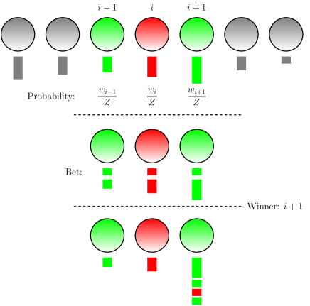
At each round, a randomly selected agent $i$ will propose a bet to her neighbors within the graph . The agent will bet a certain fraction of her power, $\alpha w_{i}$ with $\alpha<1$, and her neighbors will be required to call the bet. Neighbor players whose power is larger than $\alpha w_{i}$ are forced to do so, all others are discarded. Let ${\cal B}_{i}$ be the set of active players, whose cardinal is $m_{i}$. A winner is chosen with probability proportional to their power, i.e. the probability that player $j\in{\cal B}_{i}$ will win is

$$P_{j}={w_{j}\over Z_{i}},\qquad Z_{i}=\sum_{k\in{\cal B}_{i}}w_{k}.$$ (2)

After a winner is chosen, she earns an extra amount of power $\alpha w_{i}(m_{i}-1)$, and all others reduce their power in the amount $\alpha w_{i}$. Figure 1 provides an illustration of the basic power game procedure.

Figure 1: Top: Illustration of the power game for a one-dimensional graph. First stage: the selected agent is depicted in red, while the two neighbors appear in green, all others in gray. The bar under each player indicates her power. Second stage: players separate their bet. Third stage: a winner has been chosen (player $i+1$), and she receives all three bets. Bottom: two profiles for a system with $N=50$ and $\alpha=0.01$, for short and long times ($t=1$ and $t=1000$). Notice that, in the long run, high class agents are effectively separated by low class ones.

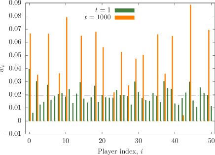
In order to determine a proper time scale, we will define a time-step as a sequence of $N$ rounds of the power game. During the first time step the homogeneous system develops random fluctuations, and these fluctuations will grow with time. In the long run, after a time of order $\alpha^{-1}$, most agents will be ruined, possessing negligible power, and a few of them will concentrate nearly all the power. A clear class division can be established in our case: agents who can call all possible bets by their neighbors are termed powerful, and correspond to the higher class. Agents who can not call some bets will be termed powerless, or lower class. In some situations, a single agent may accumulate all the power for long times.

II.1 Redistribution

In order to diminish the drive towards inequality, we may introduce a global redistribution mechanism, which we will call taxation. After each time-step, all players will provide to a central authority an amount $\tau w_{i}$ of their power, with a fixed $\tau<1$ that we will call the tax rate. The total collected amount, which is equal to $\tau$, is shared equally among them. In other words:

$$w_{i}\,\mapsto\,w_{i}-\tau w_{i}+\tau/N.$$ (3)

Notice that taxation reduces the power possessed by individuals whose power exceeds the average value, $1/N$, and increases the power of the rest. Also, notice that our proposed taxation mechanism is non-progressive, since all players must provide the same fraction of their power. It is interesting to consider $\tau^{-1}$ to be the time-scale required for the redistribution mechanism to reach an egalitarian state, starting from any distribution.

II.2 Measuring inequality

The set of $\{w_{i}\}$ will be called a profile. We define the width or roughness of the profile in similarity to the definition in kinetic roughening Barabasi :

$$W^{2}=\sum_{i=1}^{N}\left(w_{i}-\frac{1}{N}\right)^{2},$$ (4)

where we substract $1/N$ because it is the average power possessed by all agents. Notice that $W^{2}/N$ is the variance of the power.

Another useful measure of inequality is the Shannon entropy of the profile, defined by Shannon48 . Since all powers $\{w_{i}\}$ are positive and add up to one, they can be regarded as a probability distribution and we have

$$S=-\sum_{i=1}^{N}w_{i}\log w_{i}.$$ (5)

Notice that $N_{\mathrm{eff}}=\exp(S)$ can be used as an estimate for the number of active players. In effect, if we choose an agent $k$ with probability $w_{k}$, transmitting our choice will require $S$ bits, similarly to a choice among $N_{\mathrm{eff}}$ equally likely agents.

We will also consider a sorted version of the profile, $\{\omega_{i}\}$, in non-increasing order: $\omega_{1}\geq\omega_{2}\geq\cdots\geq\omega_{N}$. In other terms, $\omega_{k}$ is the power possessed by the $k$-th most powerful agent. It allows us to define the fraction of agents with power larger than $w$, $\rho(w)$, through the following relation: $\rho(w)=k/N$ when $\omega_{k}=w$. Moreover, we will define the Lorenz curve Chatterjee15 , ${\cal L}(k/N)$ is the total power possessed by the poorest $k$ players:

$${\cal L}(k/N)=\sum_{i=1}^{k}\omega_{N-i+1}.$$ (6)

The Lorenz curve allows to define the Gini coefficient Chatterjee15 of the distribution as the area between the Lorenz curve and the perfect equality value, ${\cal L}(x)=x$.

$$G\equiv\int_{0}^{1}dx\left(x-{\cal L}(x)\right).$$ (7)

It can be shown to correspond to the expected value of the differences of power of two different players, multiplied by $N$,

$$G=N\sum_{i,j=1}^{N}|w_{i}-w_{j}|.$$ (8)

In order to gather some intuition, let us consider a case where $N_{u}$ upper class agents concentrate all the power among themselves, equally. The width of the distribution can be found applying Eq. (4),

$$W^{2}={1\over N_{u}}-{1\over N}.$$ (9)

The entropy of the distribution can be found to be $S=\log(N_{u})$, expressing the amount of information required to transmit the identity of an agent selected with a probability equal to her power. On the other hand, the Gini index can be found using Eq. (7), and it is

$$G=1-{N_{u}\over N},$$ (10)

i.e. equal to the fraction of lower-class individuals.

III Two Players Game

Let us consider the case with two players, with powers $w_{1}$ and $w_{2}$. With some abuse of notation, let us call $w_{i}(t)$ the expected value for the power of the first player at time $t$. The expected amount of the bet is $\alpha/2$ ($\alpha w_{i}(t)$ when placed by player $i$). If she wins, she will gain an amount of power $\approx\alpha$, but only with probability $w_{i}(t)$. Thus, the expected value for $w_{i}(t+1)$ is given by

$$w_{i}(t+1)=w_{i}(t)+\alpha\left(w_{i}(t)-\frac{1}{2}\right).$$ (11)

This equation can be iterated, and we obtain

$$w_{i}(t)=\frac{1}{2}+\left(w_{i}(0)-\frac{1}{2}\right)(1+\alpha)^{t}.$$ (12)

In other words, the expected value of the power will increase (decrease) exponentially when the initial value is above (below) 1/2, $\exp(\pm\gamma t)$, with $\gamma=\log(1+\alpha)$.

This approach does not inform us about the fluctuations. Thus, a more detailed calculation is needed. Table 1 shows the payoff matrix for a single power game with two players, depending on who is the gambler and who is the winner.

Gambler	Winner	Probability	Payoff
$1$	$1$	$\frac{1}{2}w_{1}$	$+\alpha w_{1}$
$1$	$2$	$\frac{1}{2}(1-w_{1})$	$-\alpha w_{1}$
$2$	$1$	$\frac{1}{2}w_{1}$	$+\alpha(1-w_{1})$
$2$	$2$	$\frac{1}{2}(1-w_{1})$	$-\alpha(1-w_{1})$

Table 1: Payoff matrix for a single round of the power game between two players.

The expected gain of player 1 is given by the following expression:

$$\textrm{E}(\textrm{Gain}) = \sum\textrm{Prob.}\times\textrm{Payoff}=\alpha\left(w_{1}-\frac{1}{2}\right).$$ (13)

where the sum is implicitly extended over all possible outcomes.

In order to obtain the variance of the gain of player 1, we make use of Table 2, where we describe the expected squared deviations with respect to the expected payoff. Thus, the variance of the payoff of player 1 is given by

Gambler	Winner	Probability	$($Payoff$-$E$($Payoff$))^{2}$
$1$	$1$	$\frac{1}{2}w_{1}$	$\alpha^{2}/4$
$1$	$2$	$\frac{1}{2}(1-w_{1})$	$\alpha^{2}(4w_{1}-1)^{2}/4$
$2$	$1$	$\frac{1}{2}w_{1}$	$\alpha^{2}(4w_{1}-3)^{2}/4$
$2$	$2$	$\frac{1}{2}(1-w_{1})$	$\alpha^{2}/4$

Table 2: Fluctuations in the payoff of player 1.

$$\textrm{V}(\textrm{Payoff})=\sum\textrm{Prob.}\times\left(\textrm{Payoff}-\textrm{E}(\textrm{Payoff})\right)^{2}=\frac{\alpha^{2}}{4}$$ (14)

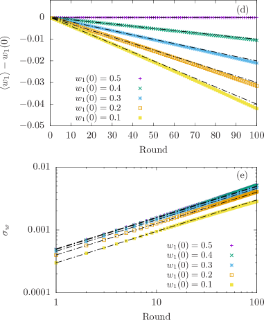
Both predictions, Eq. (13) and (14), are checked against numerical simulations in Fig. 2 (d) and (e), for a small number of rounds (100) and a low value of $\alpha=10^{-3}$. The fit is remarkably accurate.

Figure 2: Left: Two-player histogram of $w_{1}$ using $\alpha=10^{-3}$ for different initial values $w_{1}(0)=0.1$ (a), $0.3$ (b) and $0.5$ (c) and 20 games, using $10^{6}$ realizations for each case. (d) Average power of player 1 for the different initial conditions, $w_{1}(0)=0.1$ up to $0.5$ as a function of the round order. (e) Power deviation for the same cases. Notice the collapse of all curves, as predicted in Eq. (14). Dashed lines are theoretical predictions, Eqs. (13) and (the square root of) (14).

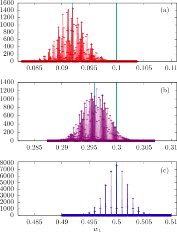
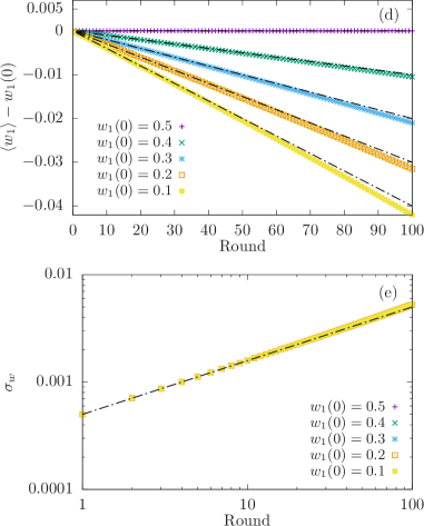
Interestingly, the collapse of all deviation curves shown in Fig. 2 (e) and predicted in Eq. (14) depends on the precise rules employed. Appendix A discusses a slightly different set of rules for which this collapse does not take place.

Notice that, in the long run, the system can be in two different absorbing states: one of the players will possess all the power while the other will be ruined. The probability of ever visiting the other state becomes negligible as the game length increases. This implies a breaking of ergodicity LZ1 ; LZ2 ; Berman17 ; Stojkovski19 : the stationary state of the system depends on its (early) history, and can not be properly called an equilibrium state.

IV One-Dimensional Power Game

The power game, as described in Sec. II, is defined on an arbitrary graph. We will consider in this section the application to a number $N$ of players displayed along a ring. For all cases, we have run $100$ simulations and averaged the results, checking for convergence.

IV.1 Without Taxes

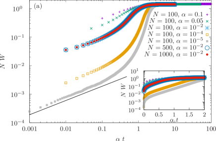
The average width of the power distribution $W$, given by Eq. (4), is shown as a function of time for different numbers of players and values of $\alpha$ in Fig. 3 (a). In all cases, the tax level was set to zero. The time axis is rescaled, as $\alpha t$, while the width axis is also rescaled, as $NW$. Notice that all curves start at zero $W$, reaching a saturation level for long times. The rescaling allows all curves to have the same saturation, independently of $\alpha$ and $N$, and a very similar saturation time. For short times, $W$ grows as a power law, $W\sim t^{1/2}$, in agreement with Family-Vicsek scaling for kinetic roughening Barabasi in the case of random deposition. Yet, before saturation the width increases much faster. The inset shows that this second stage of growth is, indeed, exponential, which does not correspond to Family-Vicsek scaling.

Figure 3: (a) Average width of the power distribution of the 1D power game as a function of time, for different values of $N$ and $\alpha$. In all cases, the tax level $\tau=0$. The time axis is rescaled as $\alpha t$, while the width axis is rescaled as $NW$, in order to highlight the collapse at saturation. (b) entropy decrease as a function of time, with the time-axis rescaled as $\alpha t$, and the entropy rescaled as $\exp(S)/N$, because this magnitude corresponds to the fraction of high class agents. Notice that this fraction comes close to $1/3$ in the long run.

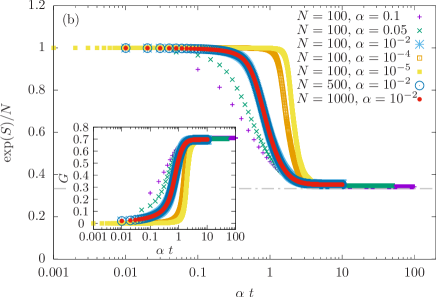
The evolution of the Shannon entropy $S$, Eq. (5), is shown in Fig. 3 (b). The time-axis is again rescaled as $\alpha t$, while the entropy is shown as $\exp(S)/N$, in order to make all curves collapse, for different values of $N$ and $\alpha$. As it was argued, $\exp(S)/N$ denotes the fraction of upper class agents, which converges to $\approx 1/3$ for long times.

The inset of Fig. 3 (b) shows the time evolution of the Gini index, with time again scaled as $\alpha t$. We notice that it evolves from $G=0$ to $G\sim 0.7$. In the class division picture, this value corresponds to the fraction of lower class agents, which should be close to $2/3$.

Thus, our observations are compatible with the conjecture that, for long times, the system is divided into an upper class, containing $\approx 1/3$ of the agents, roughly similar in power, and a lower class, with the rest of the agents. The lower class agents possess negligible power, and are unable to call the bets placed by the higher class agents. Thus, the origin of the 1/3 fraction should be understood in the following way: a stationary state is reached if each high class agent is surrounded by two lower class ones which are not neighbors of any other high class agent. A typical distribution with this property can be built by alternating one high class and two lower class agents, thus giving rise to the observed division.

Moreover, two high class agents can never be neighbors in the stationary state. That situation is unstable: in the long run, one of them will always grab the power of the other. So, when we start from a homogeneous state, the mean value of the separation between high class agents will be two in the long run. Yet, stationary states are not perfect crystals, and this separation is sometimes higher or lower. Even more: if we are allowed to start from an inhomogeneous situation, we can tune this separation to higher values. For example, an initial state with all power in the hands of one of the agents will remain stationary. Thus, we insist that our model is strongly non-ergodic.

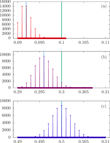
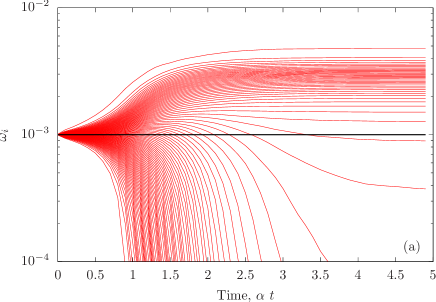
We can obtain further insight about the power distribution by considering the time evolution of the sorted profile: $\{\omega_{k}\}$, as shown in Fig. 4 (a) for $N=10^{3}$ and $\alpha=10^{-3}$. Not all values of $\omega_{k}$ are shown, only one out of every 10: $k=10m+1$. In an initial short time regime, the values diverge exponentially from the initial one, $1/N$. But for $\alpha t\sim 1$, the maximal probability $\omega_{1}$ saturates. Even before, many of the lesser agents have started an extremely fast decay.

Figure 4: (a) Time evolution of selected values of the sorted profile, $\{\omega_{k}\}$ with $k=10m+1$, using $N=10^{3}$ and $\alpha=10^{-3}$. The time axis is rescaled as $\alpha t$. Notice the initial exponential divergence, followed by saturation around $\alpha t\sim 1$. (b) and (c) Full sorted profile as a function of the index $k$, with suitably rescaled axes, for different values of time (b) and different system sizes and values of $\alpha$ in the stationary state (c).

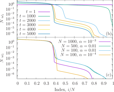
In Fig. 4 (b) and (c) we show the full sorted profile, $\{\omega_{k}\}$. Fig. 4 (b) shows these sorted profiles for different times for the previous system, $N=10^{3}$ and $\alpha=10^{-3}$. Notice that, for very short times, $N\omega_{k}\sim 1$, while it grows more and more unequal for larger times. The stationary curve has been obtained with a good approximation for $t=5000$, the last curve. For $t=1$ the sorted profile is totally flat. We see that two classes develop from the beginning, separated by a large step and with lower internal variance. As time evolves, the top part of the high class barely change, but a few high class agents fall into the lower class, as we see from the leftward shift of the class boundary with time. Fig. 4 (c) shows the stationary sorted profiles reached for different values of $N$ and $\alpha$.

The collapse of the top part of the profiles show that the parameter $\alpha$ determines the time-scale, while $N$ determines the length scale. The continuum limit is obtained for $\alpha\to 0$ and $N\to\infty$.

IV.2 With Taxes

Let us determine the effects of redistribution, through the use of taxes, as shown in Eq. (3). As we will see, a transition takes place for $\tau\sim\alpha$, from an unequal distribution to a homogeneous one, with some unexpected effects in the intermediate region.

Fig. 5 shows the width, entropy and Gini for a system with $N=10^{3}$, $\alpha=10^{-3}$ and different taxation levels. In Fig. 5 (a) we can see that the width, $W$, grows for short times as $W\sim t^{1/2}$ in all cases. For low taxation levels, $\tau<3\alpha$, it still presents the same features of the no-taxation case, with the accelerated growth of the inequality near saturation, and the saturation levels reached are similar. But above that threshold value, the behavior changes drastically, with the saturation level falling sharply after a small increase in the taxation level.

Fig. 5 (b) provides further information about this transition. We see the time evolution of the effective number of players, or size of the high class, estimated from the entropy, Eq. (5). Indeed, for $\tau<3\alpha$ this number decays steadily down to a value of order $N/3$. Yet, for $\tau\geq 3\alpha$, the effective number of players does not seem to decay, even in the long run. Thus, we conjecture that the system is not divided into classes any more. The Gini index, depicted in the inset of Fig. 5 (b), shows the same behavior: it grows steadily to a value close to $0.7$ for $\tau<3\alpha$, and remains close to zero for $\tau\geq 3\alpha$.

Yet, a careful analysis of Fig. 5 (a) and (b) holds a surprise more. Indeed, the long term $N_{\mathrm{eff}}$ is not a monotonously increasing function of $\tau$: for $\tau=\alpha$ it takes a larger value than for $\tau=2\alpha$, although just marginally so. This effect is checked carefully in Fig. 5 (c), where the stationary (long term) values of the three previous observables (width $W$, entropy $S$ and Gini $G$) are plotted as a function of the taxation level, $\tau/\alpha$. Interestingly, we observe in all three the same trend: a low taxation brings about a mild decrease in inequality. Yet, increasing the taxation level from $\tau=\alpha/2$ to $\tau=2\alpha$ increases the inequality a tiny amount. If we increase the taxation level further, inequality disappears sharply. The reason seems to be that mild levels of taxation may have a counterintuitive effect on inequality: by providing enough power to the worse-off agents, the high class agents are not effectively isolated and can still compete among themselves. Yet, we must stress that this slight uptake in the inequality rate as taxes grow is not a robust trait of the model, as we have not been able to reproduce it in higher dimensional lattices (see Sec. V).

Figure 5: (a) Average width of the 1D power game with taxes, using $N=10^{3}$ and $\alpha=10^{-3}$. The gray line stands for a $t^{1/2}$ growth. (b) Time evolution of the entropy and Gini index of the distributions. (c) Stationary values of the number of effective players, Gini index and roughness for the same systems as a function of the tax level $\tau/\alpha$.

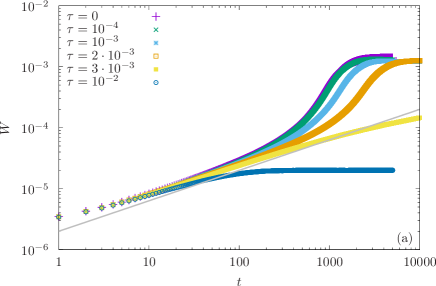
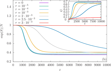
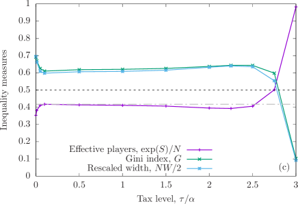
Fig. 6 (a), (b) and (c) show the time evolution of selected values of $\omega_{k}$, for $k=10m+1$. Notice that for $\tau=\alpha$, Fig. 6 (a), the evolution is very similar to the case without taxes. For $\tau=2\alpha$, Fig. 6 (b), the time axis seems to be stretched, but inequality builds up anyway. For $\tau=3\alpha$, Fig. 6 (c), on the other hand, the system is basically egalitarian, with a negliglible spread.

Figure 6: (a) to (c) Time evolution of the sorted power values, $\omega_{k}$ for selected values of $k$, with $N=10^{3}$ and $\alpha=10^{-3}$ and different taxation levels. The time axis is rescaled as $\alpha t$. (d) Stationary values of the sorted profiles for different taxation levels.

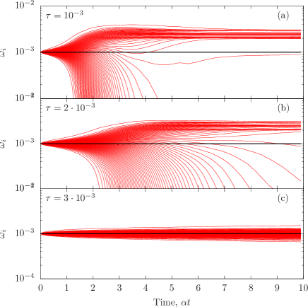
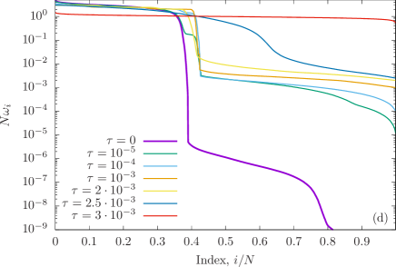
Fig. 6 (d) shows the stationary sorted profiles, $\{\omega_{k}\}$ for different taxation levels. For $\tau=3\alpha$ the profile is basically flat, but we can see that the situation can be involved for other taxation levels.

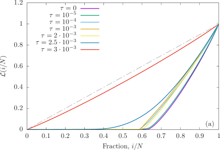
Within the economics literature, two curves present special relevance: ${\cal L}(i/N)$, the Lorenz curve, defined in Eq. (6) and the wealth function, $\rho(w)$, defined as the probability of finding an agent with power larger than $w$. The interest of these functions, which are not usual in the physics literature, is highlighted in Fig. 7. In Fig. 7 (a) we see the Lorenz curve for the aforementioned cases. Notice that the diagonal line corresponds to the case of perfect equality, while the area between the curve and the diagonal line is the Gini index. We notice that for very low taxation level the Lorenz curve is barely different from the no-taxation one, while for larger values the system changes drastically in a short span of taxation levels.

Figure 7: (a) Lorenz curves for the 1D power game with different levels of taxation, using $N=10^{3}$ and $\alpha=10^{-3}$. (b) Probability of finding an agent with power larger than $w$, as a function of $w$, for the same systems.

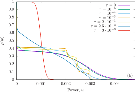
The $\rho(w)$ function is shown in Fig. 7 (b) for the same systems. We also see the strong difference achieved through a very small change in the taxation level for $\tau\sim\alpha$. For $\tau=3\alpha$ the wealth distribution $\rho(w)$ has a sharp decline around $w=1/N$, showing a basically egalitarian system. Yet, for $\tau\sim\alpha$ the curve becomes more involved, with several steps, reflecting the complex behavior of the stationary distribution for low taxation levels.

It is relevant to ask whether these results are robust under the presence of noise. We have performed numerical experiments with noisy tax rates, i.e. the tax rate for each agent becomes a random variable, uncorrelated both in space and in time. Instead of a fixed value $\tau$, the tax rate for each player at each time-step becomes $\tau_{i}=\tau(1+D\eta)$, where $D\geq 0$ is a parameter and $\eta$ is a uniform variate in $[-1,1]$. The results (not shown) are virtually identical even for values of $D\sim 1/2$. Indeed, the average value of the taxation level seems to be the only relevant variable.

V The Power Game beyond 1D

It is relevant to ask about the statistical behavior of the power distribution when the agents interact through a more complex network. In this section we will consider 1D and 2D networks with interactions beyond nearest neighbors. Concretely, we will consider 1D rings with $N$ agents, and interaction range $r=1$, 2 or 3, and periodic 2D square lattices with $L_{x}\times L_{y}=N$ agents with interaction range $r=1$ (nearest neighbors) and $r=2$ (nearest and next-nearest neighbors).

Fig. 8 shows the long-term stationary state of a power game played on a $30\times 30$ lattice with periodic boundary conditions and range $r=1$, with $\alpha=0.01$ and no taxes. The colorbox is scaled as $Nw$, where $w$ is the power of each agent, so that $Nw=1$ correspond to the initial equitative distribution. Players are still divided into two classes, and two high class players can not be together along a horizontal or vertical line in the stationary state. Yet, the configuration does not appear to present any type of long-range order. Remarkably, despite the apparent lack of a local order parameter, the number of high class players is one fifth of the total population, with a rather good precision.

Figure 8: Power profile in the steady state for a power game played on a $30\times 30$ square lattice with periodic boundaries. The color index is $Nw$, where $w$ is the power of each agent, implying that $Nw=1$ corresponds to the initial equitative level. Notice that no high-class agent is neighbor to another one, but otherwise the arrangement is disordered.

Figure 9: (a) Evolution of the expected value of the fraction of effective players, $\exp(S)/N$, as a function of rescaled-time, $K\alpha t$, where $K$ is the number of players for each round. Notice that, in the long run, the stationary fraction is always $1/K$. (b) Expected value of the fraction of effective players as a function of $\tau/(K\alpha)$ for different topologies. Notice the rather sharp increase for $\tau\sim K\alpha$, denoting the phase transition from an unequal to an egalitarian system. 1D systems operate with $N=1000$, 2D systems with $L_{x}\times L_{y}=30\times 30$, so $N=900$.

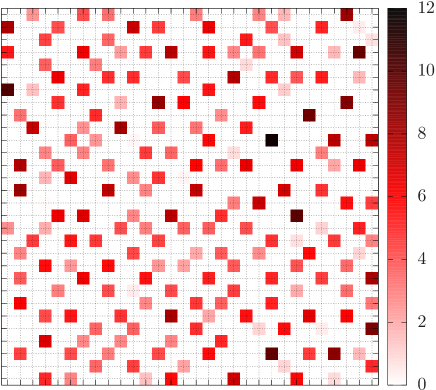
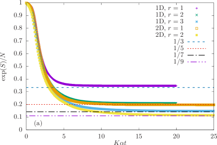
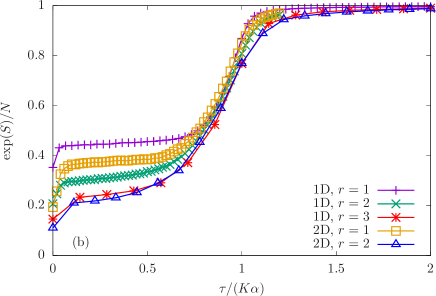
Fig. 9 (a) shows the expected value of the ratio of effective players, $\exp(S)/N$, as a function of rescaled time: $K\alpha t$, where $K$ is the number of players in each round, i.e. the coordination number plus one. In the present 2D case, $K=5$. We have plotted this average for several topologies: 1D systems with range 1, 2 and 3 interactions, and 2D systems with range 1 and 2 (next nearest neighbors, so $K=9$). In all cases, the number of effective players collapses in the short run, while its long-time behavior changes in a straightforward way: the ratio of effective players tends to $1/K$.

The short-time collapse of $\exp(S)/N$ in Fig. 9 (a) suggests that the relevant time-scale for the development of inequality in the power game is $1/(K\alpha)$. Fig. 9 (b) provides evidence to support this claim, by plotting the expected value of the long-term fraction of high class agents, $\exp(S)/N$, as a function of the ratio $\tau/(K\alpha)$ for the different system topologies explored in this section. Notice that the transition takes place for $\tau/(K\alpha)\sim 1$, i.e. when the time-scale needed to build inequality and the time-scale needed to redistribute roughly coincide.

VI Conclusions and further work

In this article we have researched a random non-strategic power game which may describe some features associated to the accretion of wealth and power in social systems. Even though the elements on which the game is based are well known in the literature (random exchanges leading to inequality and smoothing mechanisms), the extreme simplicity of the model makes it specially interesting and suitable for analysis in econophysics and in statistical mechanics.

The resource distributed among the agents is called power instead of wealth to emphasize its active character: obtaining power makes an agent more likely to obtaining even more power. In other words, the probability of winning each round is proportional to the current power in possession of each agent. Thus, small fluctuations are naturally enhanced, leading to a morphological instability. At later stages, the agents can be divided into classes: a high class, which can call all bets placed by other agents, and a lower class, which can not. Moreover, the system presents broken ergodicity: there are many possible stationary states, and an arbitrarily long waiting time is required to jump from one to another.

Importantly, the game is local: each agent can only play with her immediate neighbors. Thus, no two high class players can be neighbors in the stationary state, since one of them would ruin the other in the long run. When the players are arranged around a ring, the dynamics leads to stationary states where the number of effective players is, in average, one third of the total number of agents. For other topologies, we found evidence that the final ratio of low-to-high class players corresponds to the number of players in each neighborhood, $K$.

Starting from an equal distribution of power, early-time dynamics is described by Family-Vicsek scaling corresponding to random deposition. Yet, for longer times, the width of the interface grows exponentially, thus abandoning the Family-Vicsek paradigm. Shadowing instabilities typically lead to diffusion limited aggregation (DLA) behavior Yao.93 ; Krug.96 ; Santalla.18 , which seems to be absent from our case.

The introduction of a redistribution mechanism can revert this trend to the growth of inequality, but only if the taxation level is high enough. We can consider this effect in terms of a competition between time scales: $\tau^{-1}$ being the time scale in which redistribution acts and $(K\alpha)^{-1}$, the time scale associated to the natural growth of inequality. According to our numerical analysis, $\tau>K\alpha$ leads to an egalitarian society, with restored ergodicity, while $\tau<K\alpha$ leads to a sharp class division. This result is reminiscent of Piketty’s claim that inequality will grow when the rate of return of capital $r$ is larger than the rate of growth $g$ of the whole economy, since $r^{-1}$ and $g^{-1}$ can be thought as the time scales associated to capital and economic growth. Piketty14 ; Benisty ; Berman17b .

The above behaviours have been analyzed by using different measures for the inequality of power, such as the roughness of the profile, the Shannon entropy (which leads to a natural estimate to the number of effective players) and the Gini coefficient, always leading to similar conclusions.

Several elements have been left out in this first analysis of the power game. The first one is the characterization of the observed transition between a class society and an egalitarian society. A second one is the analysis of more realistic social network structures. In our 1D and 2D examples, we obtain evidence of a well-known fact: inequality grows with globalization. In a fragmented world, an agent can become the richest of a fixed domain, while in a fully connected world the same agent can become the wealthiest of the whole system. It is relevant to ask how our observations will change for strongly inhomogeneous lattices, more similar to human societies, such as scale-free and small-world networks.

Other interesting element to be considered in future work is the inclusion of progressive taxation, in which each player $i$ would contribute a magnitude proportional to $w_{i}^{\beta}$, leading to progressive taxation for $\beta>1$ and regressive for $\beta<1$, which will present a richer phase diagram. The role of economic initiative also leads to interesting questions: in principle, it is always against the interests of low-class players to place a bet. Thus, low-class players will only play either under coercion or under incomplete information. Coercion can be modulated through inequality itself: powerful agents may be able to force the acceptance of the bet. Yet, the role of incomplete information is specially intriguing, since it has been empirically found that a large fraction of respondents have incorrect beliefs about the inequality levels of their own country Hauser . All these possibilities are worth exploring in future work.

Appendix A Alternative set of rules for the two-player power game

As a check, we have considered an alternative version of the power game, in which the bet is fixed to $\alpha/2$ instead of being proportional to the power of the gambler. Table 3 shows the payoff matrix in this case for two players.

Gambler	Winner	Probability	Payoff
$1$	$1$	$\frac{1}{2}w_{1}$	$+\alpha/2$
$1$	$2$	$\frac{1}{2}(1-w_{1})$	$-\alpha/2$
$2$	$1$	$\frac{1}{2}w_{1}$	$+\alpha/2$
$2$	$2$	$\frac{1}{2}(1-w_{1})$	$-\alpha/2$

Table 3: Alternate power game, with a fixed bet.

Please notice that, in this variant of the game, the choice of the gambler is irrelevant, since the bet will always be the same. We can estimate in this case the expected payoff and its variance, as we did in the standard power game, obtaining the following result:

$$\textrm{E}(\textrm{Payoff}) = \alpha\left(w_{1}-\frac{1}{2}\right),$$ (15)

$$\textrm{V}(\textrm{Payoff}) = \alpha^{2}w_{1}\left(1-w_{1}\right).$$ (16)

We observe that the expected gain coincides with the standard game, but the deviation is proportional to the initial value of the power of player 1. Fig. 10 shows the histograms, expected power and deviation of the power of player 1, similarly to Fig. 2. One can see that the histogram only contains delta peaks, since the amounts of power of player 1 can only be given by $w_{1}(t)=w_{1}(0)+m\alpha$, where $m\in\mathbb{Z}$.

Figure 10: Alternate power game, with fixed bet $\alpha/2$. Left: two-player histogram of $w_{1}(t)$ using $\alpha=10^{-3}$ for different initial values $w_{1}(0)=0.1$ (a), $0.3$ (b) and $0.5$ (c) and 20 games, using $10^{6}$ realizations for each case. (d) Average power of player 1 for the different initial conditions, $w_{1}(0)=0.1$ up to $0.5$ as a function of the round order. (e) Power deviation for the same cases. Dashed lines constitute theoretical predictions, Eqs. (15) and (the square root of) (16).