Public decision support for low population density areas: An imbalance-aware hyper-ensemble for spatio-temporal crime prediction

Abstract

Crime events are known to reveal spatio-temporal patterns, which can be used for predictive modeling and subsequent decision support. While the focus has hitherto been placed on areas with high population density, we address the challenging undertaking of predicting crime hotspots in regions with low population densities and highly unequally-distributed crime.This results in a severe sparsity (i. e., class imbalance) of the outcome variable, which impedes predictive modeling. To alleviate this, we develop machine learning models for spatio-temporal prediction that are specifically adjusted for an imbalanced distribution of the class labels and test them in an actual setting with state-of-the-art predictors (i. e., socio-economic, geographical, temporal, meteorological, and crime variables in fine resolution). The proposed imbalance-aware hyper-ensemble increases the hit ratio considerably from $18.1\text{\,}\mathrm{\char 37\relax}$ to $24.6\text{\,}\mathrm{\char 37\relax}$ when aiming for the top $5\text{\,}\mathrm{\char 37\relax}$ of hotspots, and from $53.1\text{\,}\mathrm{\char 37\relax}$ to $60.4\text{\,}\mathrm{\char 37\relax}$ when aiming for the top $20\text{\,}\mathrm{\char 37\relax}$ of hotspots. As direct implications, the findings help decision-makers in law enforcement and contribute to public decision support in low population density regions.

1 Introduction

Crime inflicts immense financial losses upon individuals, businesses, and organizations, and can even threaten the stability of societies. For instance, according to recent figures from the Federal Bureau of Investigation, annual financial losses due to property crime in the United States amount to 3.6 bn USD, with an average cost of 2,361 USD per burglary. Beyond the financial damage, crime incidents are also known to trigger negative social and psychological effects, since victims suffer from a heightened level of perceived risk, which has been found to result in a significant decrease in the quality of life [Doran & Burgess, 2012]. Hence, it is the objective of decision-makers in the private and public sectors to find strategies for effective crime prevention.

In the effort to reduce crime, governments and law enforcement agencies, such as US police departments, have recently started experimenting with techniques for predictive policing in order to optimize the use of resources and to increase the chances of deterring, as well as preventing, crime events. The term “predictive policing” refers to the use of predictive analytics with the aim of identifying the potential location of criminal activity prior to such an event taking place [Ratcliffe, 2014]. Formally, this approach draws upon historical records of crime events in order to make spatio-temporal forecasts [Bowers et al., 2004, Mohler et al., 2011]. In addition, the predictive models are often extended by further information related to the socio-economic status of the resident population and to nearby points of interest (POI) [Kadar et al., 2017, Rummens et al., 2017, Vomfell et al., 2018, Wang & Brown, 2012, Xue & Brown, 2006], basic temporal variables [Rummens et al., 2017, Wang & Brown, 2012], or even social media, telecom, or mobility data [Bogomolov et al., 2014, Gerber, 2014, Kadar & Pletikosa, 2018, Vomfell et al., 2018, Wang et al., 2016], in order to better adapt to the spatio-temporal nature of crime events.

Forecasts from predictive policing improve situational awareness at both the tactical and strategic levels for law enforcement bodies and help them develop strategies for more efficient and effective policing [Perry et al., 2013, p. 2]. Figure 1 summarizes the main steps involved in deriving tactical decision support from predictive policing. In doing so, predictive policing is based on the assumption that the presence of police offers at crime hotspots leads to decreasing crime rates, which has been recently validated in randomized controlled trials [Mohler et al., 2015].

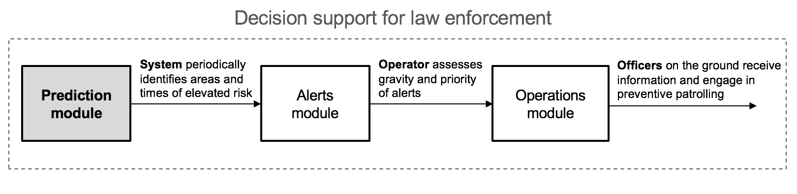
Figure 1: Schematic illustration of how predictive policing delivers spatial decision support for law enforcement.

Previous research has developed models for crime prediction that target highly populated areas. Examples include cities such as Los Angeles [Gerber, 2014], London [Bogomolov et al., 2014], and Liverpool [Bowers et al., 2004]. Other studies even narrow the focus to individual districts such as the San Fernando Valley in Los Angeles [Mohler et al., 2011]. Yet there is scant evidence that predictive policing can also be applied to areas with lower population density. In fact, prior literature has overlooked sparsely-populated regions, despite the fact that over 50 percent of household burglaries in the US occur in such areas. However, this segment of society is currently not benefiting from novel, data-driven techniques for public decision support.

The key contribution of this work is to adapt predictive policing to areas with low population density. The unique features of these regions require extensive modifications to current models used in predictive policing. More specifically, are characterized by low population densities and crime incidents that are distributed sparsely. In fact, only $0.06\text{\,}\mathrm{\char 37\relax}$ of the total daily observations in our study reflect a crime event. As a consequence, the outcome variable is affected by a severe sparsity, which, in machine learning, is called class imbalance. Due to it, traditional approaches to predictive modeling struggle achieving a forecast performance beyond a random vote. As a remedy, we follow recent suggestions for handling class imbalances, and develop a hyper-ensemble for spatio-temporal crime prediction that is specifically suited to an extreme class imbalance and, thus, to low population density areas.

Our evaluation demonstrates the capacity of crime prediction in a real-world, low population density setting. Our results reveal the challenge of forecasting spatio-temporal crime patterns with naïve predictive models, since these outperform the default hit rate of a majority vote by a mere $18.1$ percentage points in identifying the top $5\text{\,}\mathrm{\char 37\relax}$ of crime hotspots. To improve the predictive power, we propose a hyper-ensemble that combines the benefits of under-sampling and ensemble learning, thereby modeling decisive relationships between predictors and outcomes even in the presence of sparse crime events and thus extreme class imbalances. As a result, our hyper-ensemble consistently yields considerable performance improvements over common baselines: it increases the hit ratio significantly from $18.1\text{\,}\mathrm{\char 37\relax}$ to $24.6\text{\,}\mathrm{\char 37\relax}$ when aiming for the top $5\text{\,}\mathrm{\char 37\relax}$ of hotspots, and from $53.1\text{\,}\mathrm{\char 37\relax}$ to $60.4\text{\,}\mathrm{\char 37\relax}$ when aiming for the top $20\text{\,}\mathrm{\char 37\relax}$ of hotspots.

Our work entails immediate implications for decision support, especially across the public sector. This manuscript helps to further develop decision-making in public bodies by incorporating spatial analytics for data-driven decision support. Furthermore, literature commonly studies decision support in high population density regions, while neglecting a major share of the population that lives in areas with lower population density. Here we provide specific levers for translating existing prediction algorithms, such as those used for managing rescue units or traffic flow, to these settings. This is a direct remedy for an acute societal challenge, since sparsely-populated areas already experience lower average incomes and are now additionally excluded from the potential benefits of more efficient decision-making.

The remainder of this paper is structured as follows. Section 2 reviews theoretical and empirical efforts concerning crime prediction, thereby revealing the dearth of evidence in low population density environments. To close this gap, Section 3 proposes our hyper-ensemble for crime prediction in the case of extreme class imbalance. Its performance is evaluated in Section 4, revealing considerable improvements over traditional predictive models. Section 5 discusses our findings in the context of managerial implications and public decision support, while Section 6 concludes.

2 Related work

This section provides a detailed overview of the theoretical foundations, drawn from the field of criminology, based on which we motivate common choices in predictive modeling of crime incidents.

2.1 Theoretical foundation

The spatial nature of crime has been subject to extensive theory development. In this regard, under the umbrella of crime pattern theory, individual locations have been categorized according to whether they act as crime generators, crime attractors or crime detractors [Brantingham & Brantingham, 1995]. For instance, locations where large crowds assemble are supposed to serve as crime generators (e. g., sporting events), while the intrinsic characteristics of others function as crime attractors (e. g., bars) or crime detractors (e. g., police stations). In practice, these patterns can be modeled by the inclusion of points-of-interests (POIs) and other infrastructure characteristics as factors in predictive modeling, an approach that we also follow in our work. In addition, the social disorganization theory [Shaw & McKay, 1942] and its further offshoots link crime levels to the ecological attributes of the neighborhood such as socio-economic status, residential stability, and ethnic diversity. This motivates our choice of predictors in order to account for socio-demographic and economic variations among the resident population.

The temporal nature of crime is often theorized to follow two distinct patterns [Farrell & Pease, 1993]. On the one hand, the concept of repeat victimization proposes that crime events are more likely to occur at locations at which other crime incidents have previously taken place. The reason for the increased risk level originates from the assumption that offenders are more likely to exploit suitable opportunities further, for example, by stealing objects replaced after the initial theft. On the other hand, near repeat victimization refers to crime events occurring to close proximity of locations of past incidents. Here theory assumes the concept of risk heterogeneity, which states that the only association between one offense and another is the target involved. Since nearby locations of an existing crime scene are more likely to share certain characteristics, such as escape routes or levels of surveillance, it renders them potential locations for further crime in the short run. Theoretical arguments have been proposed for both patterns [Johnson, 2008], and we thus take these theories into consideration by incorporating counts of previous crime incidents into our predictive models.

Finally, the characteristics of an environment can inherently change according to climatic and seasonal conditions. A detailed literature review of different studies concerning the impact of weather-related variables on crime was performed in Murataya & Gutierrez [2013]. The fact that both violent and property crimes are significantly correlated with major holidays is documented in Cohn & Rotton [2003]. These studies have informed our choice of further temporal factors.

2.2 Crime prediction

2.2.1 Naïve predictions from historic crime data

Early attempts to identify crime hotspots relied upon non-parametric approaches, thus benefiting from simple estimation procedures but neglecting the prognostic capacity of environmental attributes and all associated spatio-temporal dynamics. For instance, the so-called spatial hotspot model applies a simple kernel density estimation to historic crime events in order to locate areas that were previously associated with a higher likelihood of criminal activity [Chainey et al., 2008]. While this approach proved feasible in high population density settings, the disparate and sparse crime events in less populated areas limit its applicability. Nevertheless, historic crime data serves as one of our baselines for determining locations with a high risk of crime. In fact, our empirical results later establish that basic models without theory-informed crime correlates result in inferior performance as compared to models leveraging spatio-temporal predictors.

2.2.2 Machine learning models with spatio-temporal predictors

Machine learning allows for the incorporation of crime correlates in order to improve prediction performance. It can thereby accommodate further theories, such as crime pattern theory and social disorganization theory. As a result, a variety of models and predictors have been proposed in the literature, which we summarize in the following (see Section 2.2.2).

There is considerable variability in terms of model choice. Past studies have quantified the probability of criminal events by means of generalized additive models [Wang & Brown, 2012], logistic regression [Gerber, 2014, Rummens et al., 2017], gradient boosting [Vomfell et al., 2018], neural networks [Rummens et al., 2017], or random forests [Bogomolov et al., 2014, Vomfell et al., 2018]. However, there is no evidence that any one model is consistently superior to all others. A potential reason might be located in the different prediction horizons, which can vary from month-ahead predictions [Bogomolov et al., 2014, Wang & Brown, 2012] and bi-weekly crime counts [Vomfell et al., 2018] to ranking hotspots on a daily basis [Gerber, 2014]. Notably, these works all deal with urban data and thus avoid having to account for class imbalance. Hence, we later experiment with a wide range of models in order to identify a tailored prediction strategy for our research setting.

Numerous spatio-temporal crime correlates have been used as predictors, often in a theory-informed manner. Location features inspired by social disorganization theory and crime pattern theory are common and predominantly include socio-demographic variables, infrastructure and POI data [Bogomolov et al., 2014, Kadar et al., 2017, Rummens et al., 2017, Vomfell et al., 2018, Wang & Brown, 2012]. To account for (near) repeat victimization, previous crime has been incorporated into the prediction models [Gerber, 2014, Wang & Brown, 2012]. Further dynamic features refer to seasonal indicators [Rummens et al., 2017], or urban human dynamics extracted from social media, mobility, or telecom data [Bogomolov et al., 2014, Gerber, 2014, Kadar & Pletikosa, 2018, Vomfell et al., 2018]. We adhere to these works and follow an extensive, theory-informed selection of spatio-temporal predictors in our low population setup.

Section 2.2.2 summarizes key studies on short-term crime prediction from the literature. We note that all studies restrict the analysis to an area with high population density (a major city or a region of it) and do not consider areas with low population density. Therefore, the novelty of this work is to expand crime prediction to low population density settings, which necessitates our hyper-ensemble, since it can successfully handle extremely imbalanced distributions of crime events.

Study	Population density	Study area	Spatial resolution	Temporal resolution	Features	Method
Bowers et al. [2004]	High	Liverpool	Grid cells of 50 m $\times$ 50 m	2 days / 1 week	Crime	Prospective hotspot
Mohler et al. [2011]	High	Part of Los Angeles	Grid cells of 200 m $\times$ 200 m	1 day	Crime	Self-exciting point processes
Wang & Brown [2012]	High	Charlottesville	Grid cells of 32 m $\times$ 32 m	1 month	Crime, spatial	Spatio-temporal generalized additive model
Gerber [2014]	High	Los Angeles	Points at 200 m $\times$ 200 m intervals	1 day	Crime, social media	Logistic regression
Bogomolov et al. [2014]	High	London metropolitan area	Lower layer super output areas (geographic hierarchy)	1 month	Crime, spatial, telecom	Random forest
Rummens et al. [2017]	High	Unnamed city in Belgium	Grid cells of 200 m $\times$ 200 m	2 weeks	Crime, spatial, temporal	Logistic regression, neural network
Vomfell et al. [2018]	High	New York City	6cmCensus tracts
(geographic hierarchy)	1 week	Crime, spatial, social media, mobility	Random forest, gradient boosting, neural network
This work	Low	Swiss canton Aargau (analogous to an US state)	Grid cells of 200 m $\times$ 200 m	1 day	Crime, spatial, temporal	Hyper-ensemble

Table 1: Key studies on short-term crime prediction (i. e., up to one month as required in tactical setups). The overview shows the dearth of works that target low population density areas. Aargau has a total surface of 140,400 hectares (1.8 times bigger than New York City) and a population density of 4.72 people/hectare (seven times less populated than New York City.

3 Methods and materials

3.1 Research framework

Low population density areas are characterized by a strong sparseness of crimes relative to the total number of instances. Such a setting where the predicted variable in machine learning is subject to sparse outcomes is termed class imbalance. That is, the number of instances from one class outnumbers the number of instances from the other class. In our particular setting, the dependent variable will be zero ($=$ no crime) almost everywhere and only set to one ($=$ crime) in $<$0.1\text{\,}\mathrm{\char 37\relax}$$ of cases. This poses a great challenge for identifying the few crime events through common predictive modeling and necessitates a tailored approach to handle such severe class imbalance.

Only a few studies in the decision support literature have investigated prediction in imbalanced datasets, either as a general methodology [Piri et al., 2018] or for specific application domains such as bankruptcy prediction [Veganzones & Séverin, 2018]. However, we later see that the traditional approach of over- or under-sampling is not sufficient in the case of such an extreme imbalance and, for this reason, we propose an imbalance-aware hyper-ensemble, which performs repeated under-sampling and should thus be more robust in identifying decisive relationships for predictive purposes.

Figure 2 summarizes our overarching research framework for identifying the most likely times and locations of burglary in a low population density environment. We investigate our proposed hyper-ensemble, but also experiment with various resampling strategies and cost-sensitive models as baselines; see the specification in the subsequent sections.

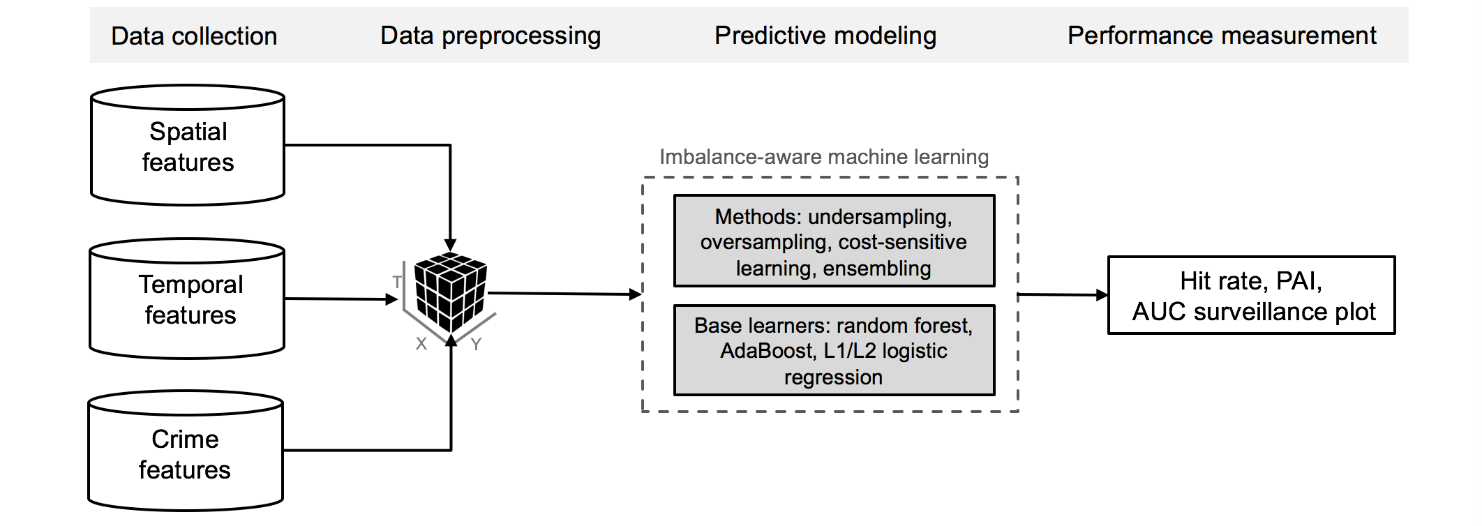
Figure 2: Research framework combining different feature sets in order to generate forecasts of crime hotspots based on imbalance-aware machine learning.

3.2 Methods for imbalance-aware machine learning

3.2.1 Proposed hyper-ensemble

Our proposed hyper-ensemble is intended to address the skewed distribution towards one class in the data and the fact that classical over- and under-sampling approaches are likely to miss discriminative information in the data. To address this and give the learning procedure additional structure, our hyper-ensemble is trained on different subsamples of the data and the test set results of these models are averaged in a final single prediction, as detailed in Algorithm 1.

Algorithm 1 Hyper-ensemble of random under-sampling models.

Training phase

1:Given training set $D_{\mathrm{train}}$ and the number of elements in the ensemble ($\phi$)

2:for $i=1$ to $\phi$ do:

3:    Create balanced sub-sample $D_{\mathrm{train}}^{i}$ of $D_{\mathrm{train}}$ by randomly drawing instances without replacement from the majority class until the same number of instances as in the minority class is reached

4:    Train model $M^{i}$ with sub-sample $D_{\mathrm{train}}^{i}$

5:end for

6:return ensemble $\{M^{1},\ldots,M^{\phi}\}$

Prediction phase

1:Given an unseen observation $\mathbold{x}$ and the ensemble $\{M^{1},\ldots,M^{\phi}\}$

2:for $i=1$ to $\phi$ do:

3:    Apply model $M^{i}$ to $\mathbold{x}$ and obtain the predicted probability $\hat{y}^{i}$

4:end for

5:return final probability whether $\mathbold{x}$ is labeled as crime or no-crime by averaging over the ensemble, i. e., $\hat{y}=\sum_{i=1}^{\phi}{\hat{y}^{i}}/\phi$

In this way, we combine the two concepts of under-sampling (i. e., adjusting the class distribution of the data set) and ensemble learning (i. e., strategically generating and combining multiple models) towards a strategy that exploits more information than a standard under-sampling approach and provides additional structure in comparison to a standard over-sampling approach.

3.2.2 Baselines

We evaluate our approach against several baselines. The most basic baseline is that of the majority class classifier – in our case this classifier will always categorize a spatio-temporal unit as no-crime (majority class). The naïve classifier baseline is that of a normal machine learning classifier, where no adjustments were made to account for the class imbalance.

In addition, a cost-sensitive learning model is implemented by proportionally increasing the cost of classification mistakes of the minority class. This classifier is trained on the entire dataset, and is an instantiation of an algorithmic approach to handling class imbalances.

We further experiment with resampling approaches to class imbalance. Random over-sampling achieves a balanced training dataset by randomly duplicating samples from the minority class until the minority class reaches the same number of samples as the majority class. In turn, random under-sampling yields a balanced training dataset by selecting a random subset of the majority class with the same size as the minority class. Heuristic over-sampling is implemented by means of SMOTE [Chawla et al., 2002], where, in order to over-sample the minority class to the size of the majority class, the following algorithm is applied: for each point $p$ in the minority class, choose a random point $r$ among its three nearest neighbors in the same class and create a random point on the line between $p$ and $r$. Heuristic under-sampling is performed by applying the NearMiss method [Yen & Lee, 2006], where, in order to reach class balance, those points in the majority class are retained that are closest to their three nearest neighbors in the minority class.

3.3 Estimation procedure

Our resampling strategies make no assumptions regarding the underling base learners, giving us the flexibility to experiment with different choices. We have evaluated different models, including regularized linear models (logistic regression with L1 and L2 regularization, i. e., LASSO and ridge logistic regressions), bagging (random forests), and boosting (AdaBoost). They all return a probability score in a binary classification setup, which we can then sort and use to compute top hotspots. We implement all of the aforementioned base learners but, for the sake of brevity, we report exhaustively the results of only one classifier, namely the random forest classifier, since it returned best results across different specifications in our experiments. This is in line with prior evidence, as random forests are known to return best benchmarking results across a multitude of problems and metrics [Caruana & Niculescu-Mizil, 2006].

We briefly summarize the idea behind the base learners in the following. Random forests are an ensemble learning method for classification, where an entire set of decision trees are grown at training time, and their mode prediction is output at testing time, thus lowering the variance of the individual trees. AdaBoost is also an ensemble model, but instead of averaging the prediction results of decision trees trained in parallel, it trains sequential decision trees, such that each new learner is optimized to correctly classify instances that have been misclassified by the previous learners. The L1 and L2 logistic regressors are simpler (i. e., linear) models with automatic regularization to avoid overfitting.

In all experiments, the dataset is split into $2/3$ training data (first two years) and $1/3$ testing data (third year). This split specifically maintains the chronological order of the data, simulating a real-world scenario and avoids over-optimistic inference [Faraway, 2016, Hirsch, 1991]. Furthermore, the classifiers are trained in a 5-fold cross validation setup on the training set in which the optimal hyper-parameters are identified, and results are always reported on the test set. Optimized parameters consist of the number and depth of the decision trees for random forest, number of trees and learning rate for AdaBoost, and regularization strength for regularized logistic regressions.

3.4 Prediction performance

For predictive policing, a decision-maker is usually interested in how many of the top hotspots were correctly identified. In machine learning, this is referred to as a ranking task. Domain-specific metrics have been proposed in the literature to evaluate spatio-temporal prediction models. The hit rate metric is the percentage of crime cells within a specified time period falling into the areas where crimes are predicted to occur [Chainey et al., 2008] and is defined as $\mathit{hit\ rate=n/N}$, where $n$ represents the number of crime areas correctly predicted, and $N$ refers to the total number of crime areas within the studied area.

The second metric with which to compare geographical prediction models is the prediction accuracy index (PAI) and has been utilized in multiple crime studies [Adepeju et al., 2016, Chainey et al., 2008, Rummens et al., 2017]. It incorporates a trade-off between the hit rate of the identified hotspots and their relative size: $\mathit{PAI\ =hit\ rate\ /coverage\ area}$. The greater the number of future crime events in a hotspot area that is smaller in size compared to the whole studied area, the higher the PAI value. The metric is controlled by the coverage area parameter, which defines what percentage of the whole area the police would be able to patrol [Adepeju et al., 2016] and is defined as $\mathit{coverage\ area=a/A}$, where $a$ is the combined area of all predicted hotspots and $A$ is the total studied area. The coverage area could be set by the decision-maker to, e. g., $5\text{\,}\mathrm{\char 37\relax}$. Therefore, in the results section, we present the metrics under different coverage area specifications. The predictions are made on a daily basis and averaged across all days in the test set.

Finally, a surveillance plot depicts the hit rate values $y$ as a function of increasing coverage area values $x$ [Gerber, 2014]. The surveillance plot is a powerful tool: if one were to monitor the top $x$ most threatened areas according to the prediction, one would observe approximately $y$ of all crimes. To produce a scalar summary for surveillance curves, we calculate their total area under the curve (AUC) [Gerber, 2014].

3.5 Data

Our crime dataset consists of burglary incidents in the Swiss canton of Aargau (i. e., analogous to a State in the US) over the course of three years from January 14, 2014 to January 13, 2017. Switzerland has consistently ranked in past several years as one of the top destinations for burglars in Europe. The canton of Aargau fits our definition of a low population area: given a total size of 140,400 hectares, it has a total population of approximately 660,000 inhabitants. Highest population densities (16 to 20 people/hectare) are achieved only in the cities of Aarau (20,000 inhabitants), Baden (17,500 inhabitants), Brugg (10,000 inhabitants), and Zofingen (10,500 inhabitants), with the majority of the environment being sparsely populated. The overall population density amounts to only 4.72 people/hectare..

Each offense in the provided crime dataset features the exact geolocation, and the reported time period in which the crime was committed. Figure 3 presents a heat map of all burglary incidents. We notice that burglary tends to cluster in three more densely populated areas, although incidents occur in less inhabited areas, as well. All burglary incidents span $32.7\text{\,}\mathrm{\char 37\relax}$ of the cantonal built surface.

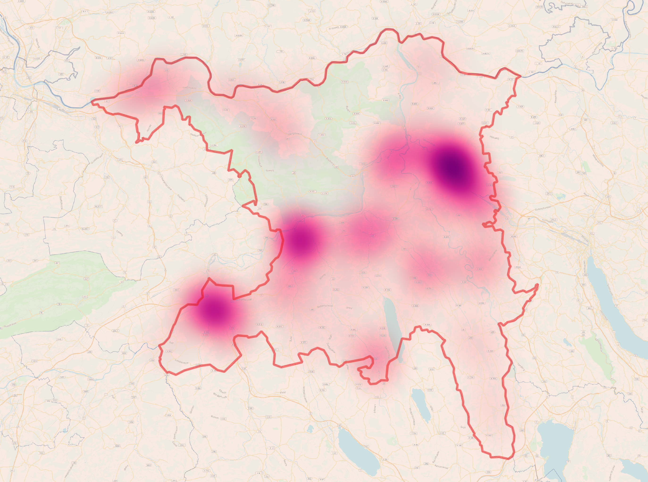
Figure 3: Heat map of burglary incidents over three years in our study setup.

We preprocess the data such that we only consider cells with built land-use where a burglary is theoretically possible, like residential and industrial areas, and exclude unbuilt land-use, like forests (see the online supplements for details). This filtering process is based on land use data provided by the cantonal geoportal AGIS and yields a final number of 10,149 grid cells that could be matched with a crime time series. Following this step, the average population density of the cells remains low at 15.6 people/hectare. This is, for instance, seven times smaller than the average population density in New York City.

Spatio-temporal data was collected with a spatial resolution of either point-level or in discretized cells of one hectare (100 m $\times$ 100 m) from the original data sources. All spatio-temporal features were then aggregated to grid cells of 200 m $\times$ 200 m with daily resolution. This choice is consistent with leading studies in the literature [Gerber, 2014, Mohler et al., 2011, Rummens et al., 2017] and was made jointly with the decision-maker, i. e., the police analyst. It was essential for the decision-maker that the spatial and temporal unit of analysis be kept at low granularity in order for the police to plan effective preventive actions. The final dataset consists of 11,123,304 spatio-temporal observations ($=$ 10,149 cells $\times$ 1,096 days), out of which only 6,266 observations are labeled as containing a burglary event. This amounts to only $0.06\text{\,}\mathrm{\char 37\relax}$ of observations of the positive class, highlighting a very severe class imbalance in the dependent variable.

Type	Theory	Name	Dimension	Description	Source
Crime	(Near) repeat victimization	prior1d, prior3d, prior7d, prior14d	integer	Number of offenses in the respective and neighboring cells in the past days	Aargau cantonal police
Locational	Social disorganization theory	popdens	people/hectare	Density of total residential population	AGIS: “Statistik der Bevoelkerung auf Hektarbasis”
		popbirth_nonCH	percent	Fraction of residents not born in Switzerland
		popcit_EU, popcit_europ, popcit_noneurop, popcit_CH	percent	Fraction of residents: EU, non-EU European, non-European, or Swiss citizens
		popcit_dividx	real between 0 and 1	Diversity of citizenship.
		pop_age1, pop_age2, pop_age3, pop_age4	percent	Fraction of residents between 0-19, 20-34, 35-64 and 65+ years of age
		popage_dividx	real between 0 and 1	Diversity of age
		popmale	percent	Fraction of male residential population
		popstab	percent	Fraction of stable residential population
		busidens	businesses/hectare	Density of workplaces	AGIS: “Statistik der Unternehmensstruktur (STATENT) 2013 auf Hektarbasis”
		busi_sec1, busi_sec2, busi_sec3	percent	Fraction of businesses in sectors 1, 2 and 3
		busisec_dividx	real between 0 and 1	Diversity of workplaces with respect to sector
		emplsec_dividx	real between 0 and 1	Diversity of employees with respect to sector
		empldens	employees/hectare	Density of employees
		emplmale	percent	Fraction of male employees
	Crime pattern theory	land_indust, land_park, land_resi1, …	percent	Fraction of land usage: industry, park, residential area with 1 story buildings, …	AGIS: “Bauzonen Schweiz (harmonisiert) Ausschnitt AG gemaess MGDM”
		land_dividx	real between 0 and 1	Diversity of land use
		buildgs_areafrac	percent	Fraction of area within a grid cell covered by buildings	AGIS: “Gebaeude ab Uebersichtsplan 1_5000”
		buildgs_dens	buildings/hectare	Density of buildings within a grid cell
		poi_infra	points/hectare	Density of infrastructural items such as ATMs, post boxes, waste baskets, etc.	OpenStreetMap Switzerland
		poi_shop	points/hectare	Density of shops
		poi_public	points/hectare	Density of public buildings such as police stations, hospitals, etc.
		poi_edu	points/hectare	Density of educational institutions such as schools, kindergartens, etc.
		poi_gastro	points/hectare	Density of gastronomical amenities such as restaurants, bars, etc.
		pub_hous	boolean	Occurrence of a public housing unit in a grid cell	Bundesamt fuer Wohnungswesen
		highway_exits	boolean	Occurrence of a highway exit within 5,000 m of the grid cell	AGIS: “Netz Kantons- strassen und Nationalstrassen”
		border_cross	boolean	Occurrence of a border crossing within 5,000 m of the grid cell
		road_type	category	Type of a road in the grid cell: from 0 = no road to 3 = high volume road
		intersection	boolean	Occurrence of a major crossroads in the respective or neighboring grid cells
		pub_trans	real between 0 and 1	Quality measure for public transport	AGIS: “OeV Gueteklassen”
Temporal	Climatic and seasonal	dow	encoded	The day of the week	—
		holiday	boolean	Indicator of whether there is a public holiday	feiertagskalender.ch
		temp	degree celsius	Temperature at 12 am	Darksky API
		hum	percent	Humidity at 12 am
		discomf	real	Discomfort index
		daylight	hours	Hours of daylight
		moon	float between 0 and 1	Moon phase (1 = full moon)
		event	integer	Number of public events on the specific day for the respective cell	events.ch

Table 2: Theory-informed choice of crime, locational, and temporal features serving as predictors.

Finally, each outcome crime/non-crime is predicted based on 64 spatio-temporal features grounded in prior criminological research and listed in Table 2. In order account for (near) repeat victimization, we craft four features based on recent crime history in the cell and its neighbors. In order to account for social disorganization theory, we formulate various socio-demographic, economical, and land-use factors from governmental open data (such as AGIS). For crime pattern theory, we exploit other open data platforms (such as OpenStreetMap) in order to describe nearby POI and road infrastructure. This amounts to a total of 52 locational features per cell. Lastly, we include eight public features that are predominantly of temporal nature and refer to calendar, weather, and event attributes of the day in each particular cell (such as the Dark Sky API).

4 Results

4.1 Overall prediction performance

Table 3 evaluates the different methods to cope with class imbalance introduced previously. The majority class model (which always predicts no crime) does not manage – by definition – to predict any hotspot. The second baseline, a random forest with no modification, achieves moderate hit rate and PAI scores. Both over-sampling techniques fail to improve upon these scores, and the first imbalance-aware technique that surpasses the baseline methods in most metrics is the heuristic under-sampling approach. It is followed by the cost-sensitive learning and random under-sampling techniques.

The best-performing method across all metrics is the hyper-ensemble. It benefits from the fact that it is trained on ten different under-sampled subsets. Through its internal model averaging, its average results outperform those of a single classifier trained on an under-sampled subset. When applied to a coverage area of $5\text{\,}\mathrm{\char 37\relax}$, the hyper-ensemble achieves a hit rate that is $35.9\text{\,}\mathrm{\char 37\relax}$ higher than the naïve baseline. It even surpasses the best baseline (i. e., random under-sampling) by $5.6\text{\,}\mathrm{\char 37\relax}$. The same pattern is also observed in the PAI scores.

When varying the coverage area, we notice that the hit rate generally improves for the models. Notably, our hyper-ensemble model consistently outperforms all baselines. The most efficient PAI is achieved at the $5\text{\,}\mathrm{\char 37\relax}$ level with a value of $4.932$.

We utilize a paired $t$-test in order to assess whether the mean hit rate and PAI results of the hyper-ensemble model are significantly better than the results of the other classifiers. We find that the results of our method are significantly better than the results of the naïve baseline at all coverage area levels ($p<0.001$). Furthermore, the hyper-ensemble also significantly outperforms the random under-sampling approach at $10\text{\,}\mathrm{\char 37\relax}$ coverage area ($p<0.05$), and at $5\text{\,}\mathrm{\char 37\relax}$ and $20\text{\,}\mathrm{\char 37\relax}$ coverage areas ($p<0.1$).

4.2 Sensitivity of prediction to base learners

We study the sensitivity with regard to different specifications of the base learners and find that the above observations, in terms of models and coverage areas, remain robust. Table 4 lists the performance of the two best model specifications (random under-sampling and hyper-ensemble of random under-sampling) with the four different base learners introduced in the previous section. We notice relatively similar performance results, whereby the random forest setup wins in most configurations, followed closely by the AdaBoost setup.

4.3 Sensitivity of prediction by population density

We study the sensitivity of the prediction performance across different levels of population density in order to understand whether there are specific regions where the model performs better (or worse). For this purpose, we split the dataset according to percentiles of the population density attribute in order to have three separate datasets with a similar number of samples: low population density ($\text{\emph{popdens}}<2.25\text{\ residents/hectare}$), medium population density ($2.25\text{\ residents/hectare}\leq\text{\emph{popdens}}\leq 16.75\text{\ residents/hectare}$), and high population density ($\text{\emph{popdens}}>16.75\text{\ residents/hectare}$). Most crime occurs in the high population density areas (i. e., 1,335 incidents), some in areas of medium population density (i. e., 398 incidents), and considerably less in low population density regions (i. e., 151 incidents).

For each subset, a model was trained analogous to the previous experiment. The performance results are listed in Table 5, revealing the following key finding: the higher the population density, the better the models are at ranking higher risk areas. Still, the overall model, having access to all data, achieves the best hit rates and PAI scores. For example, the hit rate score in the overall model outperforms the hit rate in the less populated areas by as much as $134.3\%$ and the hit rate in the more populated areas by $64.0\%$.

Classifier	5 % Coverage area		10 % Coverage area		20 % Coverage area		AUC
	Hit rate	PAI	Hit rate	PAI	Hit rate	PAI
Majority class classifier	0.0 %	0.000	0.0 %	0.000	0.0 %	0.000	0.000
Naïve classifier	18.1 %	3.621	32.5 %	3.249	53.0 %	2.651	0.754
Cost-sensitive learning	21.0 %	4.186	36.1 %	3.611	58.7 %	2.935	$0.769$
Random over-sampling	15.5 %	3.094	25.2 %	2.523	40.8 %	2.040	0.593
Random under-sampling	23.3 %	4.665	38.4 %	3.840	59.1 %	2.953	0.773
Heuristic over-sampling	16.2 %	3.252	26.5 %	2.649	41.3 %	2.063	0.590
Heuristic under-sampling	12.5 %	2.495	21.8 %	2.181	43.2 %	2.159	0.721
Hyper-ensemble	24.6 %	4.932	40.2 %	4.020	60.4 %	3.021	0.779

Table 3: Test set performance comparison of the machine learning methods proposed to cope with class imbalance. All models are trained using random forests as base learners.

Classifier	Base learner	5 % Coverage area		10 % Coverage area		20 % Coverage area		AUC
		Hit rate	PAI	Hit rate	PAI	Hit rate	PAI
Random under-sampling	Random forest	23.3 %	4.665	38.4 %	3.840	59.1 %	2.952	0.773
Random under-sampling	AdaBoost	23.2 %	4.654	37.7 %	3.771	58.7 %	2.933	0.771
Random under-sampling	L2 logistic regression	24.6 %	4.922	37.1 %	3.712	57.3 %	2.866	0.768
Random under-sampling	L1 logistic regression	21.8 %	4.363	34.1 %	3.407	54.4 %	2.717	0.758
Hyper-ensemble	Random forest	24.6 %	4.932	40.2 %	4.020	60.4 %	3.021	0.779
Hyper-ensemble	AdaBoost	23.3 %	4.659	38.1 %	3.809	59.2 %	2.959	0.772
Hyper-ensemble	L2 logistic regression	24.7 %	4.936	37.3 %	3.731	57.4 %	2.868	0.769
Hyper-ensemble	L1 logistic regression	22.1 %	4.414	34.1 %	3.409	54.5 %	2.722	0.758

Table 4: Test set performance comparison of different base learners reveals only marginal sensitivity to the choice of the base learner.

Population density	Feature set	5 % Coverage area		10 % Coverage area		20 % Coverage area		AUC
		Hit rate	PAI	Hit rate	PAI	Hit rate	PAI
All	Crime	16.1 %	3.213	27.4 %	2.743	39.0 %	1.949	0.581
	Temporal	6.5 %	1.292	12.5 %	1.255	21.1 %	1.057	0.498
	Spatial	23.3 %	4.655	37.1 %	3.711	57.2 %	2.860	0.771
	All	24.6 %	4.932	40.2 %	4.020	60.4 %	3.021	0.779
Low population density	Crime	4.0 %	0.813	5.0 %	0.508	8.0 %	0.402	0.157
	Temporal	0.7 %	0.142	3.8 %	0.385	6.5 %	0.324	0.154
	Spatial	10.5 %	2.096	15.7 %	1.568	21.2 %	1.060	0.251
	All	10.5 %	2.096	15.7 %	1.568	21.2 %	1.060	0.251
Medium population density	Crime	8.4 %	1.686	13.6 %	1.357	20.4 %	1.019	0.355
	Temporal	3.1 %	0.623	7.6 %	0.763	14.5 %	0.726	0.327
	Spatial	14.0 %	2.805	20.4 %	2.043	31.5 %	1.572	0.447
	All	15.6 %	3.123	21.5 %	2.156	29.9 %	1.493	0.448
High population density	Crime	11.6 %	2.320	21.9 %	2.185	35.1 %	1.756	0.561
	Temporal	6.0 %	1.199	11.3 %	1.132	21.7 %	1.083	0.486
	Spatial	15.1 %	3.033	23.5 %	2.348	39.2 %	1.960	0.633
	All	15.0 %	3.013	27.2 %	2.721	41.8 %	2.091	0.651

Table 5: Test set performance comparison of crime, temporal, spatial, and all features across different levels of population density. All models are trained using a hyper-ensemble of random under-sampling with random forests.

4.4 Sensitivity of prediction to temporal resolution

We also study the sensitivity with regard to the temporal resolution, by processing the target variable and the features at weekly granularity. This yields a dataset of 1,552,797 spatio-temporal observations (= 10,149 grid cells $\times$ 153 weeks) with a pronounced class imbalance of $0.56\%$ instances belonging to the positive class (i. e., crime). In this scenario, the winning hyper-ensemble of random under-sampling based on random forests achieves a total AUC of $0.844\text{\,}$ This corresponds to a hit rate of $51.9\text{\,}\mathrm{\char 37\relax}$ at $5\text{\,}\mathrm{\char 37\relax}$ coverage level, and to a hit rate of $74.4\text{\,}\mathrm{\char 37\relax}$ at $20\text{\,}\mathrm{\char 37\relax}$ coverage level. As such, weekly burglary hotspots prove to be easier to predict as daily burglary hotspots. Yet, daily predictions are desired for tactical decision-making in law enforcement.

4.5 Relevance of feature sets

Finally, we perform a direct comparison of the different predictors in terms of their predictive power for predictive policing in areas with low population density. We analyze how the prediction performance varies across three subsets of all candidate features: crime features (recent crime history in the area and surroundings), locational features (socio-demographic, land-use, POI and infrastructure factors), and primarily temporal features (calendar, weather, and event attributes). Per Table 5, we conclude that, in all areas, the locational features yield the best predictive results, approaching the results of the models with all features. This highlights the overall importance of both social disorganization theory and crime pattern theory when modeling crime patterns. Second is the model with features inferred from the recent crime incidents in the area, as per insights from (near) repeat victimization. The least predictive features turn out to be the temporal features. For instance, when training on samples spanning all population density levels, the model utilizing the complete feature set outperforms the temporal-only setting by $278.5\text{\,}\mathrm{\char 37\relax}$ and the crime-only setting by $52.8\text{\,}\mathrm{\char 37\relax}$. These results refer to the hit rate at $5\text{\,}\mathrm{\char 37\relax}$ coverage level, but, as depicted in Figure 4, the large improvement of the full model against the crime-only baseline holds at all coverage levels.

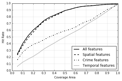
Figure 4: Surveillance plot: hit rate as a function of coverage area when considering different feature sets.

When comparing the different levels, we observe that, relative to all other zones, the spatial features perform best in the low-density areas, whereas the past crime features perform best in the high-density areas.

5 Discussion

5.1 Interpretation and link to the literature

This paper establishes the effectiveness of tailored machine learning in terms of identifying places and times of elevated burglary risk in a wide and heterogeneous region with low population density. The superior performance of the proposed hyper-ensemble can be attributed to two main factors: (1) an innovative strategy that deals with the strong class imbalance by fusing the concepts of under-sampling and ensemble learning, and (2) the incorporation of state-of-the-art spatio-temporal predictors of crime into the model.

The results achieved by our approach in a sparsely-populated environment are – despite the methodological challenges – on a par with or better than the latest results achieved in densely-populated environments, which, to their advantage, do not suffer from severe class imbalance. As an illustration, Adepeju et al. [2016] report a hit rate of $51.5\text{\,}\mathrm{\char 37\relax}$, i. e., a PAI of $2.57$, for burglary in South Chicago, while Gerber [2014] reports a hit rate of $45.0\text{\,}\mathrm{\char 37\relax}$, i. e., a PAI of $2.25$, for crime in Los Angeles, both at $20\text{\,}\mathrm{\char 37\relax}$ coverage area. Furthermore, Rummens et al. [2017] report the optimal values of $25.1\text{\,}\mathrm{\char 37\relax}$ for hit rate and $3.95$ for PAI, which were achieved at $20\text{\,}\mathrm{\char 37\relax}$ cut-off probability for home burglary in a Belgian city (this translates to approximately $6\text{\,}\mathrm{\char 37\relax}$ coverage area). Hence, our hit rate of $60.4\text{\,}\mathrm{\char 37\relax}$ at $20\text{\,}\mathrm{\char 37\relax}$ coverage area attains a similar performance, despite the more challenging setting of sparsity.

We further investigate whether the predictive performance varies across different levels of population density. We find that the presented system performs better in regions with highest levels of population density. This is not surprising, since such areas: (1) experience more crime and thus provide the algorithm with more training examples of the positive class, and (2) coincide with a wider distribution of the features, which allows the algorithm to discover more discriminative patterns.

As crime in less populated areas might not be equally affected by the different spatio-temporal factors considered, we discuss the prognostic capacity of the separate crime, spatial, and temporal feature sets. When looking at the whole study area, we find that the high number of spatial features inspired by the social disorganization and crime pattern theories predict crime best. These are followed by recent crime history features crafted according to the (near) repeat victimization phenomena, while a model trained on temporal features delivers only marginal improvement over the naïve baseline. Most importantly, the additional features describing the environment and time considerably improve the predictive power of the models relying only on crime features.

Different patterns emerge when comparing different levels of population density. In that case, the importance of past crime features increases with increasing levels of density. For instance, in less populated areas, the model based on locational features based o social disorganization theory and crime pattern theory achieves the same results as the model trained on all features, while the performance of the model based on crime features is inferior by a factor of about $2.5$. For more populated areas, the ratio shrinks to about $1.3$. his tendency is consistent with the current literature and practices in urban predictive policing, which rely heavily on insights derived from the notion of (near) repeat victimization.

5.2 Implications for management and academia

A number of studies, including randomized controlled trials, have revealed the operative potential of short-term crime prediction models [Chainey et al., 2008, Mohler et al., 2015]. In response, predictive policing solutions, such as PredPol¹⁵ and HunchLab, have been developed and integrated into the daily work of police officers in several major cities. This has led the National Research Council Committee to review research on police policies and practices, finding strong evidence that taking a focused geographic approach to the problem of crime can increase the effectiveness of policing and could lead to better public decision-making [National Research Council, 2004]. This renders our work timely and highly relevant. We contribute to this effort by studying areas with low population density that have been overlooked in previous research due to the inherent challenges of this undertaking.

Advances in big data and machine learning over the past decade have enabled the implementation of location and non-location analytics in decision support research [Pick et al., 2017] by utilizing proprietary and open data for different applications such as optimizing car-sharing [Barann et al., 2017, Willing et al., 2017], predicting crimes [Gerber, 2014, Vomfell et al., 2018], or preventing traffic accidents [Ryder et al., 2017]. Spatially-referenced data that is usually inaccessible has been made available to academic researchers, allowing us to advance the literature on location analytics for spatial decision support in smart cities [Pick, 2017], with an emphasis on under-researched regions with low population density. Furthermore, our study illustrates the successful integration of several existing theories and their innovative application to public decision-making.

The tandem of a constant increase in the ubiquity of data, in combination with exponentially advancing computational power, has led to numerous applications of big data analytics in practice. Based on the lessons learned from the digitalization of the private sector, stakeholders in the public sector are now learning how to adapt their processes and services for the 21st century – with police forces representing one example [Taylor, 2015]. Hence, the proposed methodology can be directly leveraged by decision-makers in law enforcement, both private (e. g., private security firms) and especially public (e. g., police forces). We provide a fully-fledged approach that can be integrated as a prediction module in a spatial decision support system, as the one presented in Figure 1. Based on the current available patrolling resources, a decision-maker can set the maximum coverage area and identify the top crime hotspots.

In the broader sense and inspired by our work, similar approaches utilizing imbalance-aware machine learning techniques can be envisioned to forecast other sparse spatio-temporal phenomena such as demand for prescriptions, ambulance calls, or 311/911 calls.

5.3 Limitations and potential for future research

With the goal of developing a crime prediction approach for areas with low density population, we have leveraged random forests in a hyper-ensemble approach utilizing a super-set of features that have their origins in criminological theory and empirical studies. Although random forests benefit from strong performance in this predictive setup, the resulting decision rules are largely data-driven and thus lack the same interpretability as theory. Hence, they are not the ideal instrument for testing the theoretical contribution of each individual feature – carefully crafted explanatory models and randomized controlled trials would be proper instruments if that objective was desired.

Future research could explore additional methods for highly imbalanced classifications in the domain of unsupervised learning, such as novelty detection and outlier detection. For novelty detection, the training data is not polluted by outliers, and the interest is on detecting anomalies in new observations.

Another potential avenue for future work consists of hourly crime prediction. The current limitation lies in the fact that burglaries are often discovered only post hoc. Because of that, the actual time of the burglary is unknown and can merely be approximated. With more effort on precise reporting, hourly analyses could further bolster decision support.

While we already worked with an extensive set of features that adheres to best-practice recommendations from prior research, one could potentially investigate the prognostic capacity of further features, such as, e. g., mobility or social media data, in a low population density setting. The current limitation for these datasets is their extreme sparsity in areas with low population density, making their application unfeasible at the moment. Though with the proliferation of location-based services, this might be worth revisiting in the future. In addition to expanding the feature set, it would be interesting to evaluate the presented features with respect to other types of crimes, such as theft or assaults.

6 Conclusion

The aim of this work was to explore the potential of predictive policing in a low population density setting. While areas with high population density have been subject to extensive research, decision support for law enforcement that is designed for less populated areas and their unique characteristics is scarce. Our results have demonstrated the successful application of imbalance-aware machine learning techniques to the task of building a ranking system that identifies regions and times of elevated burglary risk in a large, heterogeneous area. One of the major challenges in the prediction setup is the sparse nature of crime, which is commonly referred to as a severe class imbalance. In our study, it is coped with by proposing a hyper-ensemble that combines under-sampling and ensemble learning in an effective strategy. This approach outperforms traditional techniques based on (heuristic) under- and over-sampling, as well as cost-sensitive learning. By incorporating various spatio-temporal crime-correlating factors into the model, we significantly improve upon the predictive performance of models that rely solely on past crime data. When dividing the study area according to three different levels of population density, we notice an increase in predictive performance in areas with higher population densities. We conclude that the proposed approach can be useful for areas with low population density, which up to now have been neglected within the domain of crime forecasting.

References

References

- Adepeju et al. [2016] Adepeju, M., Rosser, G., & Cheng, T. (2016). Novel evaluation metrics for sparse spatio-temporal point process hotspot predictions - a crime case study. International Journal of Geographical Information Science, 30, 2133–2154.
- Barann et al. [2017] Barann, B., Beverungen, D., & Müller, O. (2017). An open-data approach for quantifying the potential of taxi ridesharing. Decision Support Systems, 99, 86–95.
- Bogomolov et al. [2014] Bogomolov, A., Lepri, B., Staiano, J., Oliver, N., Pianesi, F., & Pentland, A. (2014). Once upon a crime: Towards crime prediction from demographics and mobile data. In International Conference on Multimodal Interaction (pp. 427–434).
- Bowers et al. [2004] Bowers, K. J., Johnson, S. D., & Pease, K. (2004). Prospective hot-spotting: The future of crime mapping? British Journal of Criminology, 44, 641–658.
- Brantingham & Brantingham [1995] Brantingham, P., & Brantingham, P. (1995). Criminality of place. European Journal on Criminal Policy and Research, 3, 5–26.
- Canter et al. [2000] Canter, D., Coffey, T., Huntley, M., & Missen, C. (2000). Predicting serial killers’ home base using a decision support system. Journal of Quantitative Criminology, 16, 457–478.
- Caruana & Niculescu-Mizil [2006] Caruana, R., & Niculescu-Mizil, A. (2006). An empirical comparison of supervised learning algorithms. In International Conference on Machine Learning (pp. 161–168).
- Chainey et al. [2008] Chainey, S., Tompson, L., & Uhlig, S. (2008). The utility of hotspot mapping for predicting spatial patterns of crime. Security Journal, 21, 4 – 28.
- Chawla et al. [2002] Chawla, N. V., Bowyer, K. W., Hall, L. O., & Kegelmeyer, W. P. (2002). SMOTE: Synthetic minority over-sampling technique. Journal of Artificial Intelligence Research, 16, 321–357.
- Cohn & Rotton [2003] Cohn, E. G., & Rotton, J. (2003). Even criminals take a holiday: Instrumental and expressive crimes on major and minor holidays. Journal of Criminal Justice, 31, 351–360.
- Doran & Burgess [2012] Doran, B. J., & Burgess, M. B. (2012). Why Is Fear of Crime a Serious Social Problem? In Putting Fear of Crime on the Map (pp. 9–23). New York, NY: Springer New York.
- Faraway [2016] Faraway, J. J. (2016). Does data splitting improve prediction? Statistics and Computing, 26, 49–60.
- Farrell & Pease [1993] Farrell, G., & Pease, K. (1993). Once bitten, twice bitten: Repeat victimisation and its implications for crime prevention. Technical Report Home Office Police Department.
- Gerber [2014] Gerber, M. S. (2014). Predicting crime using Twitter and kernel density estimation. Decision Support Systems, 61, 115–125.
- Hirsch [1991] Hirsch, R. (1991). Validation samples. Biometrics, 47, 1193–1194.
- Johnson [2008] Johnson, S. D. (2008). Repeat burglary victimisation: A tale of two theories. Journal of Experimental Criminology, 4, 215–240.
- Kadar & Pletikosa [2018] Kadar, C., & Pletikosa, I. (2018). Mining large-scale human mobility data for long-term crime prediction. EPJ Data Science, 7, 26.
- Kadar et al. [2017] Kadar, C., Rosés Brüngger, R., & Pletikosa, I. (2017). Measuring ambient population from location-based social networks to describe urban crime. Lecture Notes in Computer Science, 10539, 521–535.
- Mohler et al. [2011] Mohler, G. O., Short, M. B., Brantingham, P. J., Schoenberg, F. P., & Tita, G. E. (2011). Self-exciting point process modeling of crime. Journal of the American Statistical Association, 106, 100–108.
- Mohler et al. [2015] Mohler, G. O., Short, M. B., Malinowski, S., Johnson, M., Tita, G. E., Bertozzi, A. L., & Brantingham, P. J. (2015). Randomized controlled field trials of predictive policing. Journal of the American Statistical Association, 110, 1399–1411.
- Murataya & Gutierrez [2013] Murataya, R., & Gutierrez, D. (2013). Effects of weather on crime. International Journal of Humanities and Social Science, 3, 71–75.
- National Research Council [2004] National Research Council (2004). Fairness and Effectiveness in Policing. Washington, DC: National Academies Press.
- Perry et al. [2013] Perry, W. L., McInnes, B., Price, C. C., Smith, S. C., & Hollywood, J. S. (2013). Predictive policing: the role of crime forecasting in law enforcement operations. Technical Report Rand Corporation.
- Pick [2017] Pick, J. B. (2017). Smart cities in the United States and worldwide: A rich arena for MIS studies. Journal of Information Technology Case and Application Research, 19, 133–144.
- Pick et al. [2017] Pick, J. B., Turetken, O., Deokar, A. V., & Sarkar, A. (2017). Location analytics and decision support: Reflections on recent advancements, a research framework, and the path ahead. Decision Support Systems, 99, 1–8.
- Piri et al. [2018] Piri, S., Delen, D., & Liu, T. (2018). A synthetic informative minority over-sampling (SIMO) algorithm leveraging support vector machine to enhance learning from imbalanced datasets. Decision Support Systems, 106, 15–29.
- Ratcliffe [2014] Ratcliffe, J. (2014). What is the future… of predictive policing? Translational Criminology, (pp. 4–5).
- Rummens et al. [2017] Rummens, A., Hardyns, W., & Pauwels, L. (2017). The use of predictive analysis in spatiotemporal crime forecasting: Building and testing a model in an urban context. Applied Geography, 86, 255–261.
- Ryder et al. [2017] Ryder, B., Gahr, B., Egolf, P., Dahlinger, A., & Wortmann, F. (2017). Preventing traffic accidents with in-vehicle decision support systems - The impact of accident hotspot warnings on driver behaviour. Decision Support Systems, 99, 64–74.
- Shaw & McKay [1942] Shaw, C. R., & McKay, H. D. (1942). Juvenile delinquency and urban areas. Chicago: University of Chicago Press.
- Taylor [2015] Taylor, J. (2015). The digital policing journey: from concept to reality realising the benefits of transformative technology. Technical Report Deloitte.
- Veganzones & Séverin [2018] Veganzones, D., & Séverin, E. (2018). An investigation of bankruptcy prediction in imbalanced datasets. Decision Support Systems, 112, 111–124.
- Vomfell et al. [2018] Vomfell, L., Härdle, W. K., & Lessmann, S. (2018). Improving crime count forecasts using Twitter and taxi data. Decision Support Systems, forthcoming.
- Wang et al. [2016] Wang, H., Kifer, D., Graif, C., & Li, Z. (2016). Crime Rate Inference with Big Data. Conference on Knowledge Discovery and Data Mining, .
- Wang et al. [2013] Wang, T., Rudin, C., Wagner, D., & Sevieri, R. (2013). Learning to detect patterns of crime. In European Conference on Machine Learning and Principles and Practice of Knowledge Discovery in Databases (pp. 515–530).
- Wang & Brown [2012] Wang, X., & Brown, D. E. (2012). The spatio-temporal modeling for criminal incidents. Security Informatics, 1, 2.
- Willing et al. [2017] Willing, C., Klemmer, K., Brandt, T., & Neumann, D. (2017). Moving in time and space – Location intelligence for carsharing decision support. Decision Support Systems, 99, 75–85.
- Xue & Brown [2006] Xue, Y., & Brown, D. E. (2006). Spatial analysis with preference specification of latent decision makers for criminal event prediction. Decision Support Systems, 41, 560–573.
- Yen & Lee [2006] Yen, S. J., & Lee, Y. S. (2006). Under-sampling approaches for improving prediction of the minority class in an imbalanced dataset. Lecture Notes in Control and Information Sciences, 344, 731–740.