Unit Commitment with Gas Network Awareness

Abstract

Recent changes in the fuel mix for electricity generation and, in particular, the increase in Gas-Fueled Power Plants (GFPP), have created significant interdependencies between the electrical power and natural gas transmission systems. However, despite their physical and economic couplings, these networks are still operated independently, with asynchronous market mechanisms. This mode of operation may lead to significant economic and reliability risks in congested environments as revealed by the 2014 polar vortex event experienced by the northeastern United States. To mitigate these risks, while preserving the current structure of the markets, this paper explores the idea of introducing gas network awareness into the standard unit commitment model. Under the assumption that the power system operator has some (or full) knowledge of gas demand forecast and the gas network, the paper proposes a tri-level mathematical program where natural gas zonal prices are given by the dual solutions of natural-gas flux conservation constraints and commitment decisions are subject to bid-validity constraints that ensure the economic viability of the committed GFPPs. This tri-level program can be reformulated as a single-level Mixed-Integer Second-Order Cone program which can then be solved using a dedicated Benders decomposition. The approach is validated on a case study for the Northeastern United States [1] that can reproduce the gas and electricity price spikes experienced during the early winter of 2014. The results on the case study demonstrate that gas awareness in unit commitment is instrumental in avoiding the peaks in electricity prices while keeping the gas prices to reasonable levels.

I Introduction

Gas-Fueled Power Plants (GFPPs) have become a significant part of the energy mix in the last decades, primarily because of their operational flexibility and lower environmental impacts. Although GFPPs have introduced interdependencies between the natural gas and electrical power systems, these networks are still operated independently, with asynchronous market mechanisms. In particular, the unit commitment decisions in the electrical power system take place before the realization of natural gas spot prices, introducing reliability risks and economic inefficiencies in congested environments. Indeed, the GFPPs may not be able to secure gas at reasonable prices, introducing either reliability issues or electricity gas spikes.

This undesirable outcome occurred in the Northeastern United States during the early winter of 2014. Extremely low temperatures induced an unusual coincident peak in electricity and natural gas demand. On the one hand, it produced record-high natural gas spot prices due to congestion. On the other hand, high electricity loads led the electrical power system operator to call for some emergency actions, which resulted in higher electricity prices [2]. Moreover, the power system operator, valuing reliability the most, encouraged committed GFPPs to buy natural gas at all costs without assurance of cost recovery, further aggravating the economic cost [3]. It is important to mention that the critical issue in this case was not the gas supply, but rather congestion in the gas transmission network. Moreover, a recent study [1] has shown that the cost of expanding the gas and network infrastructures to avoid such events would be prohibitive.

To address these interdependencies, a number of researchers have studied how to incorporate the natural gas transmission capabilities into the operational decisions of electrical power systems. See, for instance, [4, 5, 6, 7, 8, 9, 10, 11, 12, 13]. Other researchers have also studied how to incorporate the economic coupling between these two infrastructures using new market mechanisms. A new market framework with a joint ISO, using price- or volume-based approaches, was investigated in [14, 15]. Instead of introducing one joint ISO, other researchers have proposed a new market framework that assumes centralized independent gas markets, synchronizes the electricity and gas market days, and allows some information exchange between some parties in the electricity and gas markets (e.g., market operators or GFPPs) [16, 17, 18, 19, 20, 21].

This paper takes a different approach that stays within the current operating practices and does not introduce a new market mechanism. Instead, the approach generalizes the unit commitment model to capture the physical and economic couplings and strive to ensure both physical feasibility and economic viability. More precisely, the paper introduces the Unit Commitment problem with Gas Network Awareness (UCGNA) to schedule a set of generating units for the next day while taking account the fuel delivery and the natural gas prices that are propagated back by the natural gas system. The UCGNA imposes bid-validity constraints on the GFPPs to ensure their profitability and estimates the natural gas prices for these constraints with the dual solutions associated with the flux conservation constraints of the gas market.

The UCGNA is formulated as a tri-level mathematical program and assumes that the power system operator has partial (or full) knowledge on gas demand forecast and gas network. When the power system is modeled with its DC approximation and the gas network with the second-order cone program from [22] to model its steady-state physics, the tri-level mathematical program can be reformulated as a single-level Mixed-Integer Second-Order Cone Program (MISOCP) through strong duality of the innermost problem. The resulting MISOCP can then be solved using a dedicated Benders decomposition recently proposed in [23].

The key contributions of this paper are threefold. First, it proposes the first unit commitment model (UCGNA) that incorporates both the physical and economic couplings of electrical power and natural gas transmission systems and can be used within current operating practices. Second, it proposes a MISOCP that captures the UCGNA and can be solved through Benders decomposition. Finally, it demonstrates the potential of the approach on a detailed case study that replicates the behavior of the 2014 polar vortex event on the Northeastern United States. In particular, the paper shows that, on the case study, the UCGNA avoids the electricity price peaks and keeping the total gas costs reasonable, contrary to current practice, even for highly congested electrical and gas networks.

The rest of this paper is organized as follows. Section II formalizes the UCGNA and Section III presents the MISOCP. Section IV briefly reviews the solution methods for the MISOCP. Section V describes the test cases. Lastly, Section VI analyzes the behavior of the model on the case study and Section VII concludes the paper.

II Unit Commitment With Gas Awareness

This section specifies the UCGNA, including its electricity system, its natural gas network, and their physical and economic couplings. The electricity transmission grid is represented by an undirected graph $\mathcal{G}^{e}=(\mathcal{N},\mathcal{E})$ and the natural gas transmission system by a directed graph $\mathcal{G}^{g}=(\mathcal{V},\mathcal{A})$. Boldface letters represent vectors of variables, $[a,b]_{\mathbb{Z}}$ denotes the set of integers in interval $[a,b]$, and $[n]$ denotes the set $\{1,\cdots,n\}$ for some integer $n\geq 1$. The letter $\mathcal{T}$ denotes the set of time periods $\{0,1,\cdots,T\}$.

II-A The Electricity Transmission System

In the United States, Unit Commitment (UC) and Economic Dispatch (ED) problems are solved daily to determine the hourly operating schedule of generating units for the next day from bids submitted by market participants. Tables I and II summarize the parameters and variables of the UC/ED problems. With these notations, the UC model is specified in Figure 1: It is standard but is presented as a bi-level program to make the UCGNA formulations more intuitive subsequently.

TABLE I: Parameters of the Electricity System.

$\mathcal{G}^{e}=(\mathcal{N},\mathcal{E})$	Undirected graph where $\mathcal{N}$ is a set of buses indexed by $i=1,\cdots,N$ and $\mathcal{E}$ is a set of lines indexed with $e=1,\cdots,E$
$\mathcal{U}$	Set of generators, indexed by $u=1,\cdots,U$
$\quad\mathcal{U}^{g}\subseteq\mathcal{U}$	Set of GFPPs
$\quad\mathcal{U}(i)\subseteq\mathcal{U}$	Set of generators located at $i\in\mathcal{N}$
$\mathcal{B}_{u}$	Set of supply bids submitted by $u\in\mathcal{U}$, indexed by $b=1,\cdots,B_{u}$
$\quad\beta_{b}$	Bid price of $b\in\mathcal{B}_{u}$
$\quad\overline{s}_{b}$	Amount of real power generation of $b\in\mathcal{B}_{u}$
$\underline{p}_{u},\overline{p}_{u}$	Minimum/maximum real power generation of $u\in\mathcal{U}$
$\underline{R}_{u},\overline{R}_{u}$	Ramp-down/-up rate of $u\in\mathcal{U}$
$c_{u}$	No-load cost of $u\in\mathcal{U}$
$\Psi_{u}$	Set of counts of time periods with distinct start-up costs of $u$ indexed by $h$
$\quad{C}_{u,h}$	Start-up cost of $u\in\mathcal{U}$ when $u$ is turned on after it has been offline for some time $\in[\Psi_{u,h},\Psi_{u,h+1}]$
$\overline{u}_{u,0},\overline{p}_{u,0}$	Initial on-off status/real power generation of $u\in\mathcal{U}$
$\underline{\tau}_{u},\overline{\tau}_{u}$	Minimum-down/-up time of $u\in\mathcal{U}$
$\underline{\tau}_{u,0},\overline{\tau}_{u,0}$	The time that generator $u\in\mathcal{U}$ has to be inactive/active from $t=0$
$b_{e}$	Line susceptance of $e\in\mathcal{E}$
$\overline{f}_{e}$	Real power limit of $e\in\mathcal{E}$
$(d^{e}_{i,t})_{i\in\mathcal{N}}$	Electricity load profile during $t\in\mathcal{T}$
$\Delta_{e}$	Maximum voltage angle difference between two end-points of $e\in\mathcal{E}$
$\underline{\theta}_{i},\overline{\theta}_{i}$	Minimum/maximum voltage angle at $i\in\mathcal{N}$

TABLE II: Variables of the Electricity System.

Binary variables
$u_{u,t}$	1 if $u\in\mathcal{U}$ is on during $t\in\mathcal{T}$, 0 otherwise
$v^{+}_{u,t}$	1 if $u\in\mathcal{U}$ becomes online during $t\in\mathcal{T}$, 0 otherwise
$v^{-}_{u,t}$	1 if $u\in\mathcal{U}$ becomes offline during $t\in\mathcal{T}$, 0 otherwise
Continuous variables
$s^{e}_{b,t}$	Real power generation from $b\in\mathcal{B}_{u}$ of $u\in\mathcal{U}$ during $t\in\mathcal{T}$
$p_{u,t}$	Real power generation of $u\in\mathcal{U}$ during $t\in\mathcal{T}$
$f_{e,t}$	Real power flow on $e\in\mathcal{E}$ during $t\in\mathcal{T}$
$r_{u,t}$	Start-up cost of $u\in\mathcal{U}$ during $t\in\mathcal{T}$
$\theta_{i,t}$	Voltage angle on $i\in\mathcal{N}$ during $t\in\mathcal{T}$

$$\min\ \sum_{t\in[T]}\sum_{u\in\mathcal{U}}(c_{u}u_{u,t}+r_{u,t}+\sum_{b\in\mathcal{B}_{u}}\beta_{b}{s}^{e}_{b,t})$$ (1a)

s.t. $$r_{u,t}\geq C_{u,h}(u_{u,t}-\sum_{n\in[h]}u_{u,t-n}),$$

$$\hskip 86.72267pt\forall h\in\Psi_{s},u\in\mathcal{U},t\in[T],$$ (1b)

$$r_{u,t}\geq 0,\ \forall u\in\mathcal{U},t\in[T],$$ (1c)

$$u_{u,t}=\overline{u}_{u,0},\ \forall u\in\mathcal{U},\ t\in[0,\overline{\tau}_{u,0}+\underline{\tau}_{u,0}]_{\mathbb{Z}},$$ (1d)

$$\sum_{t^{\prime}\in[t-\overline{\tau}_{u}+1,t]_{\mathbb{Z}}}v^{+}_{u,t^{\prime}}\leq u_{u,t},$$

$$\hskip 43.36464pt\forall u\in\mathcal{U},\ t\in[\max\{\overline{\tau}_{u},\overline{\tau}_{u,0}+1\},T]_{\mathbb{Z}},$$ (1e)

$$\sum_{t^{\prime}\in[t-\underline{\tau}_{u}+1,t]_{\mathbb{Z}}}v^{+}_{u,t^{\prime}}\leq 1-u_{u,t-\underline{\tau}_{u}},$$

$$\hskip 43.36464pt\forall u\in\mathcal{U},\ t\in[\max\{\underline{\tau}_{u},\underline{\tau}_{u,0}+1\},T]_{\mathbb{Z}},\$$ (1f)

$$v^{+}_{u,t}-v^{-}_{u,t}=u_{u,t}-u_{u,t-1},\forall u\in\mathcal{U},\ t\in[T],$$ (1g)

$$v^{+}_{u,t},v^{-}_{u,t},u_{u,t}\in\{0,1\},\forall u\in\mathcal{U},\ t\in[T],$$ (1h)

$$\boldsymbol{s}^{e}=\mbox{argmin}\ \mathcal{Q}(\boldsymbol{u},\boldsymbol{v}^{+},\boldsymbol{v}^{-}),$$ (1i)

where $$\mathcal{Q}(\boldsymbol{u},\boldsymbol{v}^{+},\boldsymbol{v}^{-})$$ denotes the ED problem specified as follows:

$$\min \sum_{t\in[T]}\sum_{u\in\mathcal{U}}\left(\sum_{b\in\mathcal{B}_{u}}\beta_{b}{s}^{e}_{b,t}\right)$$ (1j)

s.t. $$\sum_{u\in\mathcal{U}(i)}{p}_{u,t}-d^{e}_{i,t}=\sum_{e\in\mathcal{E}:e_{t}=i}f_{e,t}-\sum_{e\in\mathcal{E}:e_{h}=i}f_{e,t},$$

$$\hskip 108.405pt\ \forall i\in\mathcal{N},\ t\in[T],$$ (1k)

$${p}_{u,t}=\sum_{b\in\mathcal{B}_{u}}{s}^{e}_{b,t}\ \forall u\in\mathcal{U},\ t\in[T],$$ (1l)

$$0\leq s^{e}_{b,t}\leq\overline{s}_{b},\ \forall b\in\mathcal{B}_{u},\ u\in\mathcal{U},\ t\in[T],$$ (1m)

$$\underline{p}_{u}u_{u,t}\leq p_{u,t}\leq\overline{p}_{u}u_{u,t},\ \forall u\in\mathcal{U},\ t\in[T],$$ (1n)

$$p_{u,0}=\overline{p}_{u,0},\ \forall u\in\mathcal{U},$$ (1o)

$$p_{u,t}-p_{u,t-1}\leq\overline{R}_{u}u_{u,t-1}+\overline{p}_{u}v^{+}_{u,t},\ \forall u\in\mathcal{U},\ t\in[T],$$ (1p)

$$p_{u,t-1}-p_{u,t}\leq\underline{R}_{u}u_{u,t-1}+\underline{p}_{u}v^{-}_{u,t},\ \forall u\in\mathcal{U},\ t\in[T],$$ (1q)

$$f_{e,t}=-b_{e}(\theta_{e_{h},t}-\theta_{e_{t},t}),\ \forall e\in\mathcal{E},\ t\in[T],$$ (1r)

$$-\overline{f}_{e}\leq f_{e,t}\leq\overline{f}_{e},\ \forall e\in\mathcal{E},\ t\in[T],$$ (1s)

$$\underline{\theta}_{i}\leq\theta_{i,t}\leq\overline{\theta}_{i},\ \forall i\in\mathcal{N},\ t\in[T],$$ (1t)

$$-\Delta_{e}\leq\theta_{e_{h},t}-\theta_{e_{t},t}\leq\Delta_{e}\ \forall e\in\mathcal{E},\ t\in[T].$$ (1u)

Figure 1: The Unit Commitment and Economic Dispatch Models.

The objective function of the upper level problem (Equations (1a) - (1h)) includes the no-load costs, the start-up costs, and the costs of the selected supply bids of each electrical power generating units. Equation (1b) computes the start-up cost $r_{u,t}$ of a generator $u$ for time period $t$ based on how long $u$ has been offline. The expression $u_{u,t}-\sum^{h}_{n=1}u_{u,t-n}$ is one when generator $u$ becomes online after it has been turned off for $h$ time periods. Equation (1c) states the nonnegativity requirement on $r_{u,t}$. Equation (1d) specifies the initial on-off status of each generator. The minimum-up and -down constraints are specified in Equations (1e) and (1f) respectively. The relationship between the variables for the on-off, start-up, and shut-down statuses of each generator is stated in Equation (1g). The binary requirements for logical variables $v^{+}_{u,t},v^{-}_{u,t},u_{u,t}$ are specified in Equation (1h).

Based on the commitment decisions, the lower-level problem (i.e., Equations (1j) - (1u)) decides the hourly operating schedule of each committed generators in order to minimize the system production costs. Equation (1k) states the flow conservation constraints for real power at each bus, using $e_{h}$ and $e_{t}$ to represent the head and tail of $e\in\mathcal{E}$. Equation (1l) states that the total real power generation of a generator $u$ is equal to the production of its selected bids. Equation (1m) constrains the power generation $s_{b,t}^{e}$ from bid $b\in\mathcal{B}_{u}$ to be no more than the submitted amount $\bar{s}_{b}$. Equation (1n) enforces the bound on the real power generation of each generator. Equation (1o) specifies the initial generation amount of each generator, and Equations (1p) and (1q) state the ramp-up and -down constraints of each generator. Equation (1r) captures the DC approximation of the power flow equations and Equation (1s) specifies the thermal limit on each line. Equations (1t) and (1u) state the voltage angle bounds on each bus and the bounds on the angle difference of two adjacent buses respectively.

II-B The Natural Gas Transmission System

TABLE III: Parameters of the gas system

$\mathcal{G}^{g}=(\mathcal{V},\mathcal{A})$	Directed graph representing a natural gas transmission network, where $\mathcal{V}$ is a set of junctions, indexed with $j=1,\cdots,V$, and $\mathcal{A}\subseteq\mathcal{V}\times\mathcal{V}$ is a set of connections, indexed with $a=1,\cdots,A$
$\quad\mathcal{A}_{c}\subseteq\mathcal{A}$	Set of compressors
$\quad\mathcal{A}_{v}\subseteq\mathcal{A}$	Set of control valves
$\kappa_{j}$	Cost of demand shedding at $j\in\mathcal{V}$
$(d^{g}_{j,t})_{j\in\mathcal{V}}$	Gas demand profile during $t\in\mathcal{T}$
$\underline{s}^{g}_{j},\overline{s}^{g}_{j}$	Lower/Upper limit on natural gas supply at $j\in\mathcal{V}$
$c_{j}(\cdot)$	Cost function for gas supply at $j\in\mathcal{V}$
$W_{a}$	Pipeline resistance (Weymouth) factor of $a\in\mathcal{A}$
$\underline{\pi}_{j},\overline{\pi}_{j}$	Minimum/maximum squared pressure at $j\in\mathcal{V}$
$\underline{\alpha}^{c}_{a},\overline{\alpha}^{c}_{a}$	Lower/upper compression ratio of $a\in\mathcal{A}_{c}$
$\underline{\alpha}^{v}_{a},\overline{\alpha}^{v}_{a}$	Lower/upper control ratio of $a\in\mathcal{A}_{v}$

TABLE IV: Variables of the gas system

$s^{g}_{k,t}$	Amount of gas supplied by $k\in\mathcal{K}$ during $t\in\mathcal{T}$
$\pi_{j,t}$	Pressure squared at $j\in\mathcal{V}$ during $t\in\mathcal{T}$
$\phi_{a,t}$	Gas flow on $a\in\mathcal{A}$ during $t\in\mathcal{T}$
$l_{j,t}$	Satisfied gas demand at $j\in\mathcal{V}$ during $t\in\mathcal{T}$
$q_{j,t}$	Shedded gas demand at $j\in\mathcal{V}$ during $t\in\mathcal{T}$
$\gamma_{j,t}$	Total amount of gas consumed by the GFPP located at $j\in\mathcal{N}\cap\mathcal{V}$ during $t\in\mathcal{T}$

$$\min\ \sum_{t\in[T]}\sum_{j\in\mathcal{V}}(\sum_{s\in\mathcal{S}_{j}}c_{j,s}s^{g}_{s,t}+\kappa_{j}q_{j,t})$$ (2a)

s.t. $$s^{g}_{j,t}-l_{j,t}-\gamma_{j,t}=\sum_{a\in\mathcal{A}:a_{t}=j}\phi_{a,t}-\sum_{a\in\mathcal{A}:a_{h}=j}\phi_{a,t},$$

$$\hskip 108.405pt\forall j\in\mathcal{V},t\in[T],$$ (2b)

$$l_{j,t}=d^{g}_{j,t}-q_{j,t},\forall j\in\mathcal{V},t\in[T],$$ (2c)

$$0\leq q_{j,t}\leq d^{g}_{j,t},\forall j\in\mathcal{V},t\in[T],$$ (2d)

$$\phi_{a,t}\geq 0,\forall a\in\mathcal{A},t\in[T],$$ (2e)

$$\underline{s}^{g}_{j}\leq s^{g}_{j,t}\leq\overline{s}^{g}_{j},\forall j\in\mathcal{V},\ t\in[T],$$ (2f)

$$\underline{\alpha}^{c}_{a}\pi_{a_{h},t}\leq\pi_{a_{t},t}\leq\overline{\alpha}^{c}_{a}\pi_{a_{h},t},\forall a\in\mathcal{A}_{c},\ t\in[T],$$ (2g)

$$\underline{\alpha}^{v}_{a}\pi_{a_{h},t}\leq\pi_{a_{t},t}\leq\overline{\alpha}^{v}_{a}\pi_{a_{h},t},\forall a\in\mathcal{A}_{v},\ t\in[T],$$ (2h)

$$\pi_{a_{h},t}-\pi_{a_{t},t}=W_{a}\phi_{a,t}^{2},\forall a\in\mathcal{A}\setminus(\mathcal{A}_{v}\cup\mathcal{A}_{c}),\ t\in[T],$$ (2i)

$$\underline{\pi}_{j}\leq\pi_{j,t}\leq\overline{\pi}_{j},\forall j\in\mathcal{V},\ t\in[T]$$ (2j)

$$s^{g}_{j,t}=\sum_{s\in\mathcal{S}_{j}}s^{g}_{s,t}$$ (2k)

Figure 2: The Natural Gas Transmission Model.

Tables III and IV specify the parameters and variables of the steady-state natural gas model, which is given in Figure 2. The modeling is similar to those in [1, 22, 24] and uses the Weymouth equation to capture the relationship between pressures and flux. The flux conservation constraint is given in Equation (2b), where $a_{h}$ and $a_{t}$ represent the head and tail of $a\in\mathcal{A}$. Equation (2c) determines the demand served at each junction: It captures the amount of gas load shedding which must be nonnegative and cannot exceed the demand at the corresponding junction (Equation (2d)). The model assumes that gas flow directions are predetermined and Equation (2e) enforces the sign of gas flow variables, i.e., it constrains $\phi_{a,t}$ to be nonnegative. Equation (2f) specifies the upper and lower limits of natural gas supplies. The change in pressure through compressors and control valves are formulated in Equations (2g) and (2h) and the model use a single compressor machine approximation as in prior work. The steady-state physics of gas flows is formulated with the Weymouth equation in Equation (2i). Equation (2j) states the bounds on nodal pressures. Equation (2i) can be convexified using the second-order cone relaxation from [24]: $\pi_{a_{h},t}-\pi_{a_{t},t}\geq W_{a}\phi_{a,t}^{2}.$ This relaxation is very tight [24].

When the gas system is not congested, the price of natural gas is relatively stable. However, during congestion and when some loads are being shedded, natural gas prices increase sharply. The cost of gas in the objective function captures this behavior: For a junction $j$, it is specified with an almost-linear piecewise linear function for production and a high penalty cost $\kappa_{j}$ for gas shedding. To be specific, let $\mathcal{S}_{j}$ be a set of non-overlapping intervals covering $[0,\overline{s}^{g}_{j}]$, each with a distinct slope $c_{j,s}$ satisfying $c_{j,s}\leq c_{j,s+1}$ whenever $s,s+1\in S_{j}$. Define an auxiliary nonnegative variable $s^{g}_{s,t}$ that represents the amount of gas supply from $s\in S_{j}$ at time $t$. The objective function is then stated as

$$\sum_{t\in[T]}\sum_{j\in\mathcal{V}}(\sum_{s\in\mathcal{S}_{j}}c_{j,s}s^{g}_{s,t}+\kappa_{j}q_{j,t}).$$

The model also includes constraint (2k) to link the gas variable at junction $j$ with the auxiliary variables.

II-C Physical and Economic Couplings

GFPPs are the physical and economic interface between the electrical power and gas networks. This section first describes the resulting coupling constraints before describing how the natural gas zonal prices are computed. Tables V and VI describe the parameters for the coupling.

TABLE V: Parameters for the Electricity and Gas Coupling.

$\{H_{u,i}\}_{i=0,1,2}$	Coefficients of the heat rate curve of $u\in\mathcal{U}^{g}$
$\alpha_{u}$	Maximum allowable percentage of the expense on natural gas over its marginal bid price for $u\in\mathcal{U}^{g}$
$\mathcal{K}$	Set of pricing zones, indexed with $k=1,\cdots,K$
$\quad\mathcal{V}(k)$	Set of junctions that belong to $k\in\mathcal{K}$

TABLE VI: Variables for the Electricity and Gas Coupling.

$w_{b,t}$	1 if $b\in\mathcal{B}_{u}$ of $u\in\mathcal{U}$ is selected during $t\in\mathcal{T}$, 0 otherwise
$\rho_{u,t}$	Price of marginally selected bid of $u\in\mathcal{U}^{g}$ during $t\in\mathcal{T}$
$\psi_{k,t}$	Zonal price of natural gas in $k\in\mathcal{K}$ during $t\in\mathcal{T}$

The physical couplings between $\mathcal{G}^{e}$ and $\mathcal{G}^{g}$ can be formulated as follows ($t\in[T],j\in\mathcal{N}\cap\mathcal{V}$):

$$\gamma_{j,t}=\sum_{u\in\mathcal{U}(i)\cap\mathcal{U}^{g}}H_{u,2}p_{u,t}^{2}+H_{u,1}p_{u,t}+H_{u,0}.$$ (3)

The real power generation $\boldsymbol{p}$ of a GFPP induces a demand $\boldsymbol{\gamma}$ in the natural gas system. Equation (3) specifies the relationship between the real power generation of a GFPP and the amount of natural gas needed for the generation. In the equation, this relationship is approximated by a quadratic heat-rate curve, whose coefficients are given as $H_{u}$. The equation can be convexified like the Weymouth equation.

Since the level of power generation of the GFPPs determines the load in the gas system, the physical coupling also affects the natural gas prices. The price formation of natural gas, in turn, governs the profitability of GFPPs, which submit bids before the realization of gas prices. To capture these economic realities, the model introduces binary variables of the form $w_{b,t}\in\{0,1\}$ for each bid $b$ of a GFPP: Variable $w_{b,t}$ indicates whether bid $b$ is selected during time period $t$. Equation (1l) is then replaced by the following constraints (for all $t\in[T]$):

$$\rho_{u,t}=\sum_{b\in[B_{u}-1]}\beta_{b}(w_{b,t}-w_{b+1,t})+\beta_{B_{u}}w_{B_{u},t},\forall u\in\mathcal{U}^{g},$$ (4a)

$$0\leq s^{e}_{b,t}\leq\overline{s}_{b},\forall b\in\mathcal{B}_{u},\ u\in\mathcal{U}\setminus\mathcal{U}^{g},$$ (4b)

$$0\leq s^{e}_{b,t}\leq\overline{s}_{b}w_{b,t},\forall b\in\mathcal{B}_{u},\ u\in\mathcal{U}^{g}$$ (4c)

$$w_{b,t}\leq u_{u,t},\forall b\in\mathcal{B}_{u},\ u\in\mathcal{U}^{g},$$ (4d)

$$\overline{s}_{b}w_{b+1,t}\leq s_{b,t},\forall b\in[1,B_{u}-1]_{\mathbb{Z}},\ u\in\mathcal{U}^{g}.$$ (4e)

Equations (4b) and (4c) are bound constraints for the bids submitted by the non-GFPPs and GFPPs respectively. Equation (4c) ensures that the indicator variable $w_{b,t}$ is one whenever bid $b$ is used for time period $t$ (i.e., $s^{e}_{b,t}>0$). Equation (4d) states that the bid of a generator can be selected only when it is committed and Equation (4e) ensures that the $(b+1)^{\mbox{th}}$ bid is selected only if the bid $b$ is fully used. Accordingly, Equation (4a) states that $\rho_{u,t}$ is the maximum/marginal bid price of GFPP $u\in\mathcal{U}^{g}$ among its currently selected bids.

The economic coupling between the electricity and gas networks is enforced by bid-validity constraints that ensure that the marginal costs of producing electricity by GFPPs are lower than their marginal bid prices. Although the natural gas system is operated in a decentralized manner, the zonal price of natural gas $\boldsymbol{\psi}$ can be modeled as a function $g$ of the market supply and demand, i.e., as a function of the binary and continuous variables of Problems (1) and (2), which are denoted by $\boldsymbol{z}$ and $\boldsymbol{x}$. Under this assumption, the bid validity constraints can be expressed as follows (for all $t\in[T]$):

$$\psi=g(z,x),$$ (5a)

$$\alpha_{u}\rho_{u,t}+M(1-u_{u,t})\geq\left[2p_{u,t}H_{u,2}+H_{u,1}\right]\psi_{k,t},$$

$$\hskip 56.37271pt\forall k\in\mathcal{K},i\in\mathcal{V}(k),u\in\mathcal{U}(i)\cap\mathcal{U}^{g}.$$ (5b)

They capture the fact that, when the realized natural gas price

$$\left[2p_{u,t}H_{u,2}+H_{u,1}\right]\psi_{k,t}$$

for generating one additional unit of real power by GFPP $u$ is greater than its marginal bid price $\rho_{u,t}$, GFPP $u$ is not profitable. This situation arises because GFPP $u$ submits its bids before the realization of $\boldsymbol{\psi}$. The bid validity constraint is expressed in Equation (5b) and ensures that only profitable GFPPs are committed. The bid validity constraints use the realized zonal gas prices from Equation (5a) and $M$ denotes a big-M value set to the maximum natural gas price (e.g., $200 per mmBtu) multiplied by $\left[2\overline{p}_{u}H_{u,2}+H_{u,1}\right]$.

It remains to specify how to compute the zonal gas prices, i.e., the function $g$ in Equation (5a). The UCGNA assumes that the nodal natural gas price at each junction $j$ is given by the marginal cost of supplying natural gas at $j$. This marginal cost is the dual solution associated with the corresponding flux conservation constraint in Problem (2). The zonal natural gas prices $\boldsymbol{\psi}$ are then computed by averaging the nodal natural gas prices of a subset of junctions in the zone. Therefore, the zonal natural gas price $\boldsymbol{\psi}$ are given by linear functions of the dual solution to Problem (2).

Note that, by construction, the natural gas zonal prices $\boldsymbol{\psi}$ under normal operating conditions are given by the almost linear part of objective (2a). However, when the gas network is congested and load needs to be shed, the zonal prices increase sharply due to the high penalty cost $\kappa_{j}$. As a result, the resulting model closely captures the behavior of the market during the 2014 polar vortex. Note also that the model does not shed the demand of the GFPPs. The model assumes that GFPPs buy natural gas at any cost to meet its commitment obligation. Once again, this captures the 2014 Polar Vortex situation where GFPPs were encouraged to buy the natural gas from the spot market at any cost for the sake of the power system reliability [3].

III Reformulation of the UCGNA

This section shows how the UCGNA can be expressed as a MISOCP. Let variable subscripts $p$ and $g$ respectively denote the power and the gas systems. Let $\boldsymbol{z}_{p}$ and $\boldsymbol{x}_{p}$ respectively denote the vector of binary and continuous variables of the power system (i.e., Problem (1)) and let $\boldsymbol{x}_{g}$ be the vector of continuous variables of the gas system (i.e., Problem (2)). The UCGNA can be stated as a trilevel program:

$$\min_{\underset{\boldsymbol{z}_{p}\in\{0,1\}^{m}}{\boldsymbol{x}_{p}\geq 0,\boldsymbol{y}_{g}}}\quad c_{p}^{T}\boldsymbol{x}_{p}+h^{T}\boldsymbol{z}_{p}$$ (6a)

s.t. $$\;\;\;\boldsymbol{z}_{p}\in\mathcal{Z},$$ (6b)

$$\begin{array}[]{lcl}(\boldsymbol{x}_{p},\boldsymbol{y}_{g})=&\underset{\boldsymbol{x}_{p}\geq 0,\boldsymbol{y}_{g}}{\mbox{argmin}}&c_{p}^{T}\boldsymbol{x}_{p}\\ &\mbox{s.t.}&A\boldsymbol{x}_{p}+B\boldsymbol{z}_{p}\geq b,\\ &&\boldsymbol{y}_{g}\in\mbox{Dual sol. of }\eqref{TL:g},\\ \end{array}$$ (6f)

$$\;\;\;E\boldsymbol{y}_{g}+M\boldsymbol{z}_{p}\geq h$$ (6g)

where $\mathcal{Z}$ denotes the feasible region of the unit commitment problem (i.e., Equations (1b)-(1h)), the third level problem is defined as

$$\underset{\boldsymbol{x}_{g}\in\mathcal{K}}{\min}\ c_{g}^{T}\boldsymbol{x}_{g}:D_{p}\boldsymbol{x}_{p}+D_{g}\boldsymbol{x}_{g}\geq d,$$ (7)

and $\mathcal{K}$ is the proper cone denoting the domain of $\boldsymbol{x}_{g}$.

The first-level problem (i.e., Equations (6a) and (6b)) formulates the unit-commitment problem (i.e., Equations (1a)-(1h) and Equation (4)). The unit-commitment decisions $\boldsymbol{z}_{p}$ from the first-level problem are then plugged into the second-level problem, which formulates the economic dispatch problem (i.e., Equations (1j)-(1u)) and decides the hourly operating schedule of committed generating units. Then, the third-level problem (i.e., Problem (7)) formulates the natural gas problem (i.e., Problem (2) and Equation (3)) and determines the resulting nodal prices for natural gas based on the dual solution $\boldsymbol{y}_{g}$ of the economic dispatch decisions.

Equations (6a), (6b), and (6f) capture the current operating practice of the power system. The first level captures the commitment decisions that are taken first without consideration of the gas network. The second and third levels implement a Stackelberg game, where the dispatch decisions of the electricity system are followed by those of the natural gas network. The novelty in the UCNGA is the bid-validity constraint (6g), which corresponds to Equation (5b): It ensures that only profitable GFPPs are selected in the first level and uses the dual variables of the third-level problem to do so, allowing the unit-commitment problem to anticipate the zonal prices of natural gas.

The following theorem, whose proof is in Appendix A, shows that the tri-level problem can be reformulated as a single-level mathematical program. The proof uses strong duality on the third-level problem and a lexicographic optimization to merge the second and third levels.

Theorem 1

Problem (6) can be asymptotically approximated by the following mathematical program:

$$\min\ \alpha h^{T}\boldsymbol{z}_{p}+\alpha c_{p}^{T}\boldsymbol{x}_{p}+(1-\alpha)c_{g}^{T}\boldsymbol{x}_{g}$$ (8a)

s.t. $$\boldsymbol{z}_{p}\in\mathcal{Z},$$ (8b)

$$A\boldsymbol{x}_{p}+B\boldsymbol{z}_{p}\geq b,$$ (8c)

$$D_{p}\boldsymbol{x}_{p}+D_{g}\boldsymbol{x}_{g}\geq d,$$ (8d)

$$\boldsymbol{y}_{p}^{T}(b-B\boldsymbol{z}_{p})+\boldsymbol{y}_{g}^{T}d\geq\alpha c_{p}^{T}\boldsymbol{x}_{p}+(1-\alpha)c_{g}^{T}\boldsymbol{x}_{g},$$ (8e)

$$\boldsymbol{y}_{g}^{T}D_{g}\preceq_{\mathcal{K}^{*}}(1-\alpha)c_{g}^{T},$$ (8f)

$$\boldsymbol{y}_{p}^{T}A+\boldsymbol{y}_{g}^{T}D_{p}\leq\alpha c^{T}_{p},$$ (8g)

$$\frac{1}{1-\alpha}E\boldsymbol{y}_{g}+M\boldsymbol{z}_{p}\geq h,$$ (8h)

$$\boldsymbol{x}_{p}\geq 0,\boldsymbol{x}_{g}\in\mathcal{K},\boldsymbol{y}_{p}\geq 0,\boldsymbol{y}_{g}\geq 0,$$ (8i)

$$\boldsymbol{z}_{p}\in\{0,1\}^{m},$$ (8j)

for some $\alpha\in(0,1)$. Moreover, when $\alpha\rightarrow 1$, the optimal solution of Problem (8) converges to the optimal solution of Problem (6).

Observe that Problem (8) has a bilinear term of $\boldsymbol{y}_{p}^{T}B\boldsymbol{z}_{p}$ in Equation (8e). Assuming that $\boldsymbol{y}$ has an upper bound of $\overline{\boldsymbol{y}}$, this term can be rewritten using an exact McCormick relaxation to produce a MISOCP.

Remark 1

Problem (8) is best viewed as a “standard” MISOCP to which a constraint on the dual variables of its inner-continuous problem has been added. The “standard” MISOCP optimizes the joint electricity and natural gas problem

$$\min\ \alpha h^{T}\boldsymbol{z}_{p}+\alpha c_{p}^{T}\boldsymbol{x}_{p}+(1-\alpha)c_{g}^{T}\boldsymbol{x}_{g}$$ (9a)

s.t. $$\boldsymbol{z}_{p}\in\mathcal{Z},$$ (9b)

$$A\boldsymbol{x}_{p}+B\boldsymbol{z}_{p}\geq b,$$ (9c)

$$D_{p}\boldsymbol{x}_{p}+D_{g}\boldsymbol{x}_{g}\geq d,$$ (9d)

$$\boldsymbol{x}_{p}\geq 0,\boldsymbol{x}_{g}\in\mathcal{K},\boldsymbol{z}_{p}\in\{0,1\}^{m},$$ (9e)

and the additional constraints

$$\frac{1}{1-\alpha}Ey_{g}+Mz_{p}\geq h.$$

on the dual variables $(y_{p},y_{g})$ of its inner continuous problem capture the bid validity.

IV Solution Approach

This section briefly sketches how the MISOCP is solved. Problem (8) can be reformulated as

$$\underset{\boldsymbol{z}_{p}\in\mathbb{B}^{n}}{\min}\ \alpha h^{T}\boldsymbol{z}_{p}+f(\boldsymbol{z}_{p})$$ (10a)

s.t. $$\boldsymbol{z}_{p}\in\mathcal{Z}.$$ (10b)

where

$$f(\boldsymbol{z}_{p})=\ \min\alpha c_{p}^{T}\boldsymbol{x}_{p}+(1-\alpha)c_{g}^{T}\boldsymbol{x}_{g}$$ (11a)

s.t. $$A\boldsymbol{x}_{p}+B\boldsymbol{z}_{p}\geq b,$$ (11b)

$$D_{p}\boldsymbol{x}_{p}+D_{g}\boldsymbol{x}_{g}\geq d,$$ (11c)

$$\boldsymbol{y}_{p}^{T}(b-B\boldsymbol{z}_{p})+\boldsymbol{y}_{g}^{T}d\geq\alpha c_{p}^{T}\boldsymbol{x}_{p}+(1-\alpha)c_{g}^{T}\boldsymbol{x}_{g},$$ (11d)

$$\boldsymbol{y}_{g}^{T}D_{g}\preceq_{\mathcal{K}^{*}}(1-\alpha)c_{g}^{T},$$ (11e)

$$\boldsymbol{y}_{p}^{T}A+\boldsymbol{y}_{g}^{T}D_{p}\leq\alpha c^{T}_{p},$$ (11f)

$$\frac{1}{1-\alpha}E\boldsymbol{y}_{g}+M\boldsymbol{z}_{p}\geq h,$$ (11g)

$$\boldsymbol{x}_{p}\geq 0,\boldsymbol{x}_{g}\in\mathcal{K},\boldsymbol{y}_{p}\geq 0,\boldsymbol{y}_{g}\geq 0.$$ (11h)

The implementation applies a Benders decomposition on this formulation to solve Problem (8). Moreover, the dual of Problem (11) has a special structure that can be exploited by the dedicated Benders decomposition from [23]. The idea is to decompose the dual of Problem (11) into two more tractable problems. The extreme points and rays of these subproblems can be used to find the (feasibility and optimality) Benders cuts of Problem (11). The solution method also uses the acceleration schemes from [25, 26] which normalize the rays $\hat{y}$ and perturb $\hat{z}_{p}$. The solution method also obtains feasible solutions periodically (e.g., every 30 iterations) heuristically by turning off violated generators. Finally, the solution method applies a preprocessing step to eliminate some invalid bids. It exploits the fact that the natural gas prices without the GFPP load gives a lower bound on the natural gas zonal prices. Therefore, the implementation solves Problem (2) with no GFPPs, i.e., $\gamma_{j,t}=0$ for all $j\in\mathcal{V},t\in[1,T]_{\mathbb{Z}}$. Those bids violating the bid-validity constraint with regard to these zonal prices are not considered further.

V Description of the Data Sets

The UCGNA model is evaluated on the gas-grid test system from [1], which is representative of the natural gas and electric power systems in the Northeastern United States. This test system is composed of the IEEE 36-bus NPCC electric power system [27] and a multi-company gas transmission network covering the Pennsylvania-To-Northeast New England area in the United States [1]. The data for the test system can be found online at https://github.com/lanl-ansi/GasGridModels.jl.

The test system consists of 91 generators of various types (e.g., hydro, gas-fueled, coal-fired, nuclear, etc.). The unit-commitment data for these generators (e.g., generator offer curves including start-up and no-load costs and operational parameters such as minimum run time) was obtained from the RTO unit commitment test system [28]. Each generator in the gas-grid test system is assigned the unit commitment data adapted to its fuel-type and megawatt capacity.

The gas-grid test case consists of two natural gas pricing zones: Transco Zone 6 non NY and Transco Leidy Line. The Transco Leidy Line represents the natural gas prices in the Marcellus Shale production area, which has a wealth of natural gas. On the other hand, the Transco Zone 6 non NY represents the natural gas prices near consumption points. Therefore, a large difference in prices between these two pricing zones implies a scarcity of transmission capacities between these two points. During normal operations, the average natural gas prices in the Transco Zone 6 non NY and the Leidy Line are around $3/mmBtu and $1.5/mmBtu respectively. The slopes $c_{j,s}$ at junction $j\in\mathcal{V}$ (see Section (II-B)) are chosen to be around these numbers. The penality cost for load shedding $\kappa_{a}j$ is set as $130/mmBtu for all junctions. The results are given for a single time-period (i.e., $T=1$).

VI Case Study

This section analyzes, under various operating conditions, the behavior of the UCGNA on the realistic test system described in Section V. The results are compared with current practices. The case study varies the level of stress on both the electrical power and gas systems. For the electrical power system, the load is uniformly increased by 30% and 60%. For the gas system, the load is uniformly increased by 10% up to 130%. Parameters $\eta_{p}$ and $\eta_{g}$ respectively represent the stress level imposed on the electrical power and gas systems. In the results, (A) denotes existing practices and (B) the UCGNA model. Solutions for (B) are obtained with a wall-clock time limit of 1 hour, while solutions for (A) is obtained by the following procedure:

1. Solve the power model (i.e., Problem (1));

2. Retrieve the demand of GFPPs using Equation (3) and plug it into the gas model (i.e., Problem (2));

3. Solve the gas model and compute the natural gas zonal prices using the dual values associated with the flux conservation constraints;

4. Based on the zonal prices, determine the set of GFPPs violating the bid-validity constraint (i.e., Equation (5b)) and compute the loss of such GFPPs by multiplying the violation, i.e., the difference between the marginal gas price and the marginal bid price, with the scheduled amount of power generation.

The behaviors of (A) and (B) in the normal, stressed, and highly-stressed power systems are compared in Figures 3, 4, and 5 respectively. In each figure, (a) and (c) display the system costs and natural gas prices of (A), and (b) and (d) display those of (B). More precisely, (a) and (b) present the total cost breakdown in terms of the cost of electrical power system, the cost of the gas system, and the economic loss from invalid bids. (c) and (d) depict the natural gas zonal prices in each pricing zone.

(a) System costs (A).

(b) System costs (B).

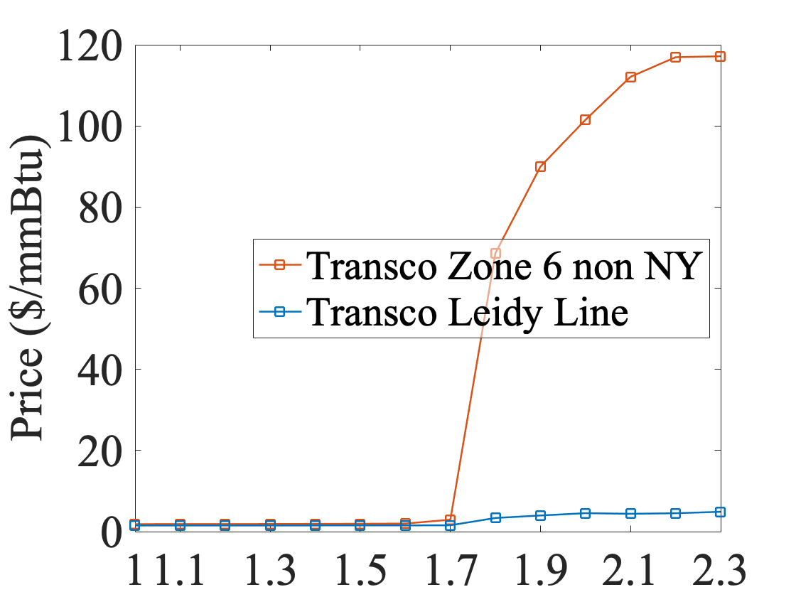
(c) Natural gas prices (A).

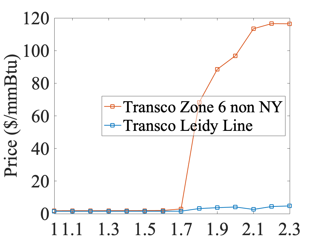
(d) Natural gas prices (B).

Figure 3: Results for the Normal Operating Conditions of the Electrical Power System ($\eta_{p}=1$).

Figures 3a and 3c show that the gas system cost gradually increases as $\eta_{g}$ increases up to $1.7$, then it grows rapidly from $\eta_{g}=1.8$ on. The rapid increase is due to load shedding (see Section II-B) and leads to natural gas price spikes in Transco Zone 6 non NY. The large difference between the prices in Zone 6 and Leidy Line indicates that the load shedding occurs due to the lack of transmission capacity between these two points, not because of a lack of gas supply. Due to the gas price spike in Transco Zone 6 non NY, some bids of GFPPs become invalid and incur some losses, which increases the total cost. On the other hand, for (B), the electrical power system cost is slightly higher than for (A), but it does not incur any economic loss from invalid bids and the overall cost is lower. Observe also that model (A) captures the same behavior as in the 2014 polar vortex. Additionally, observe that the gas price in the Zone 6 region is also exhibiting sharp increases in model (B). However, this peak has significantly less impact for (B) given the different commitment decisions.

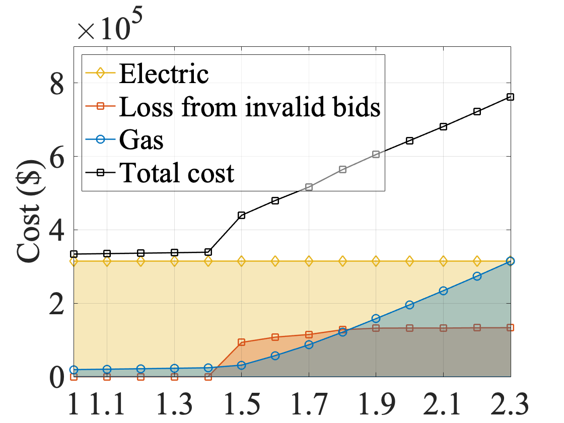
(a) System costs (A).

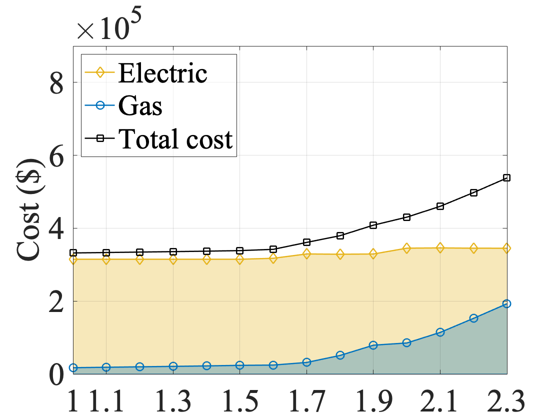
(b) System costs (B).

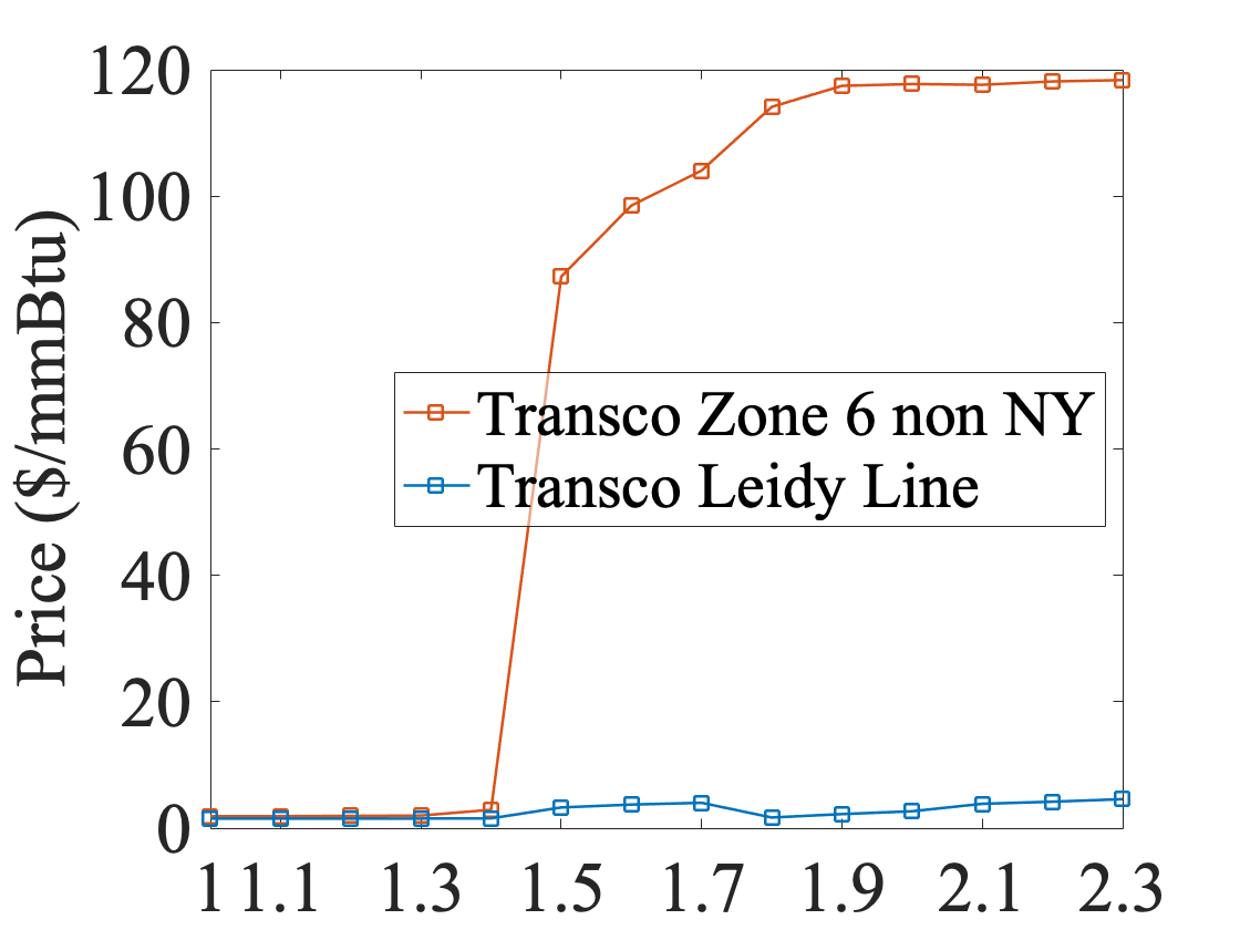
(c) Natural gas prices (A).

(d) Natural gas prices (B).

Figure 4: Results for the Stressed Electrical Power System ($\eta_{p}=1.3$).

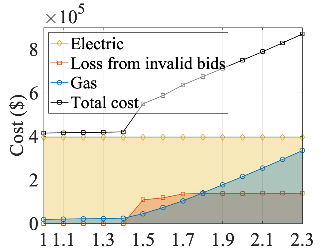
(a) System costs (A).

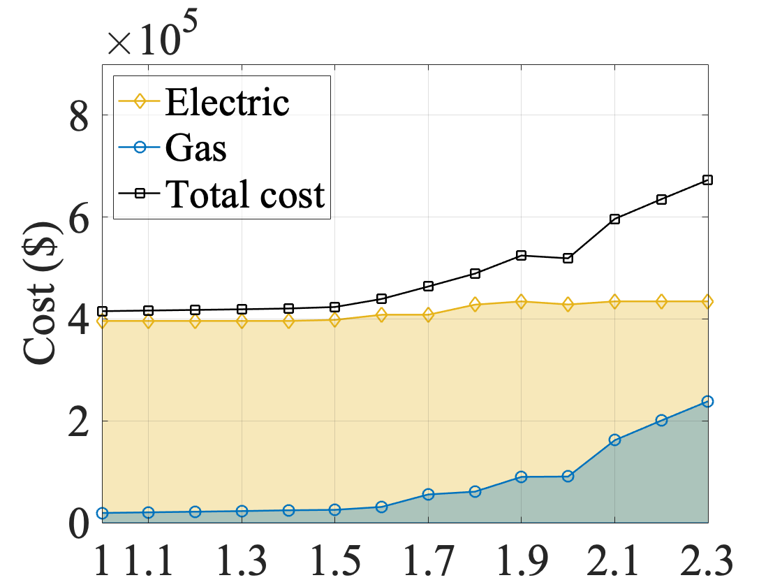
(b) System costs (B).

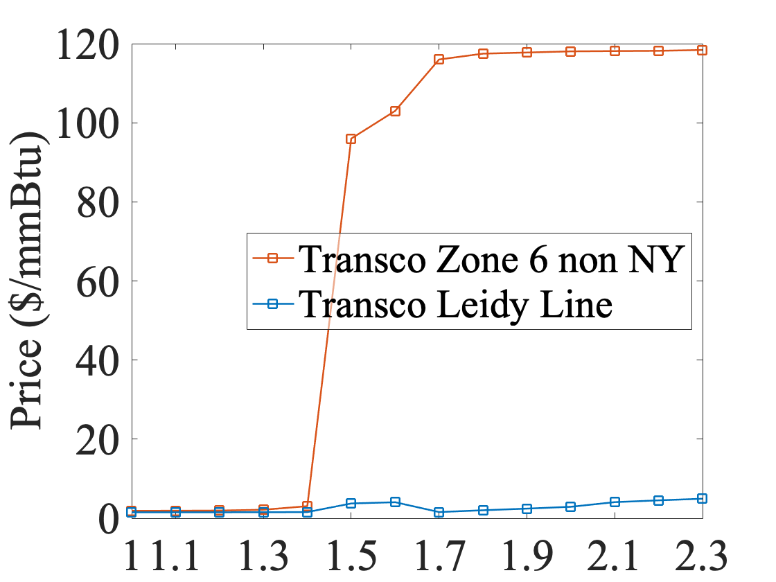
(c) Natural gas prices (A).

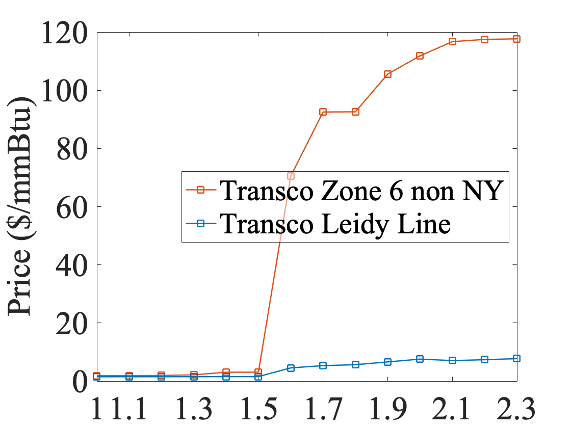
(d) Natural gas prices (B).

Figure 5: Results for the Highly-Stressed Electrical Power System ($\eta_{p}=1.6$).

The differences in behavior between systems (A) and (B) become clearer as the load increases in the electrical power system. For the stressed power system, displayed in Figure 4, the difference between the total cost of (A) and (B) becomes very large: There are many invalid bids for (A), which puts the reliability of the power system at high risk and induces an electricity price peak. The price of gas and the economic losses both increase significantly in (A) and the increases start at stress level 1.5 for the gas network. In contrast, (B) maintains a reliable operation independently of the stress imposed on the natural gas system. The price of gas increases obviously but less than in (A) and the cost of the power system remains stable. The peak in gas price only starts at stress level 1.7, showing that (B) delays the impact of congestion in the gas networks by making better commitment decisions.

Figure 5 shows the benefits of (B) over (A) become even more substantial when both systems are highly stressed. Observe that the cost of the electrical power system remains stable once again in (B) and that the cost of the gas network increases reasonably. In contrast, Model (A) exhibits significant increases in gas prices and economic cost from invalid bids. These results indicate that bringing gas awareness in unit commitment brings significant benefits in congested networks. By choosing commitment decisions that ensure bid validity, the UCGNA brings substantial cost and reliability benefits for congested situations like the 2014 polar vortex.

TABLE VII: Statistics on Committed Generators for the Stressed Electrical Power System ($\eta_{p}=1.6$): The first 7 columns display the number of committed generators with respect to its fuel type, where (O) Oil, (C) Coal, (G) Gas, (H) Hydro, (R) Refuse, (N) Nuclear, (E) Others, and the last two columns show the number of committed GFPPs in each pricing zone, where (T) Transco Zone 6 Non NY and (L) Transco Leidy Line.

$\eta_{g}$	(O)	(C)	(G)	(H)	(R)	(N)	(E)	(T)	(L)
1.0	7	6	12	11	0	12	3	8	4
1.6	8	6	10	11	0	13	3	6	4
2.3	9	6	9	11	0	13	3	4	4

(a) Number of committed GFPPs (A).

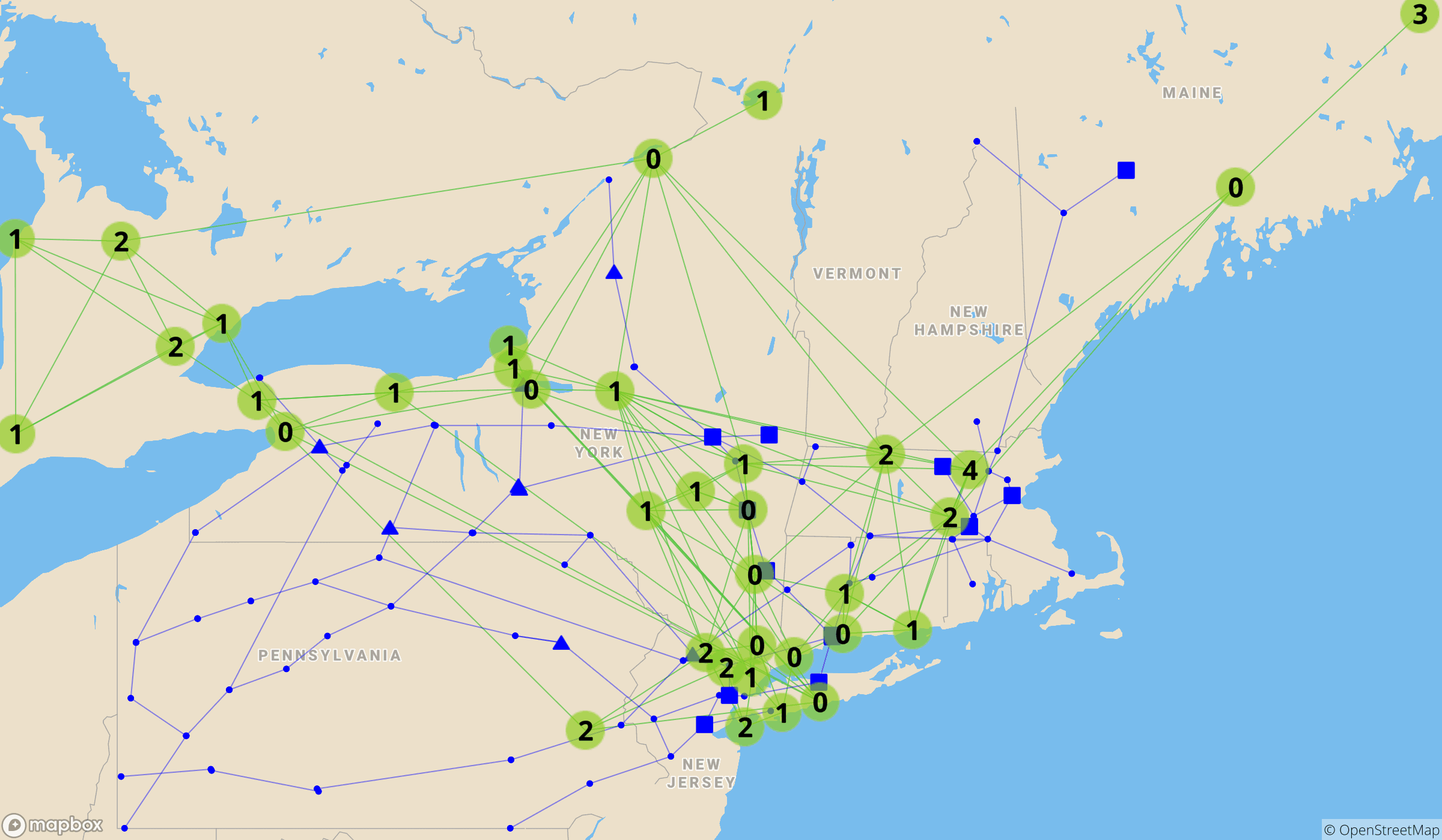
(b) Number of committed non-GFPPs (A).

(c) Number of committed GFPPs (B).

(d) Number of committed non-GFPPs (B).

Figure 6: Results for the Highly-Stressed Condition ($\eta_{p},\eta_{g}$) = (1.6,2.3).

TABLE VIII: Solution Statistics for (B).

	1		1.3		1.6
	(i)	(ii)	(i)	(ii)	(i)	(ii)
1	255301.0	0.0	332123.0	0.0	415315.0	0.0
1.1	256502.0	0.0	333333.0	0.0	416530.0	0.0
1.2	257706.0	0.0	334548.0	0.0	417759.0	0.0
1.3	258915.0	0.0	335776.0	0.0	419015.0	0.0
1.4	260132.0	0.0	337036.0	0.0	420548.0	0.0
1.5	261364.0	0.0	338564.0	0.0	423466.0	0.0
1.6	262613.0	0.0	342066.0	0.3	439254.0	2.1
1.7	264019.0	0.0	361089.0	3.5	463746.0	2.0
1.8	278679.0	1.8	379532.0	3.2	489011.0	6.2
1.9	296251.0	1.3	408407.0	3.3	524533.0	7.4
2	317619.0	0.0	430415.0	4.2	519026.0	3.7
2.1	329801.0	0.0	460127.0	4.3	596449.0	5.0
2.2	358828.0	0.0	497952.0	4.0	635128.0	5.0
2.3	405022.0	0.0	537874.0	0.0	672876.0	0.0

The great cost and reliability benefits of (B) are owing to better commitment decisions that anticipate the future state of the gas system. Table VII summarizes some statistics on committed generators under the highly stressed power system. As the gas load increases, some of the GFPPs in (T) are no longer committed and the lost generation is replaced by generators of different types or GFPPs with reasonable bid prices. More specifically, Figure 6 shows the commitment decision of (A) and (B) for ($\eta_{p},\eta_{g}$) = (1.6,2.3). The numbers in black in Figures 6a and 6c report the number of committed GFPPs on the corresponding bus; Those in Figures 6b and 6d display the number of committed non-GFPPs. In Figure 6a, the numbers in red on the bottom right corner of some buses represent the number of committed GFPPs located at the bus without bid validity. Most invalid GFPPs in Figure 6a are turned off in Figure 6c and replaced by some non-GFPPs as Figure 6d indicates.

Finally, Table VIII summarizes the objective value and the optimality gap of (B) for each instance. For 16 out of 42 instances, the algorithm times out (wall-clock limit time of 1 hour) and it reports sub-optimal solutions whose optimality gaps are presented in columns denoted by (ii). It is important to stress however that even sub-optimal solutions to the UCGNA bring significant benefits for gas-grid networks as shown previously.

VII Conclusion

The 2014 polar vortex showed how interdependencies between the electrical power and gas networks may induce significant economic and/or reliability risks under heavy congestion. This paper has demonstrated that these risks can be effectively mitigated by making unit commitment decisions informed by the physical and economic couplings of the gas-grid network. The resulting Unit Commitment with Gas Network Awareness (UCGNA) model builds upon the standard unit commitment used in current practices but also reasons about the feasibility of gas transmission feasibility and the profitability of committed GFPPs. In particular, the UCGNA introduces bid-validity constraints that ensure the economic viability of committed GFPPs, whose marginal bid prices must be higher than the marginal natural gas prices. The UCGNA is a three-level model whose bid validity constraints operate on the dual variables of flux conservation constraints in the gas network, which represent the marginal cost of gas for producing a unit of electricity. It can be formulated as a Mixed-Integer Second-Order Cone Program (MISOCP) and solved using a dedicated Benders decomposition approach. The case study, based on a modeling of the gas-grid network in the North-East of the United States, shows that the UCGNA has significant benefits compared to the existing operations: It is capable to ensure valid bids even at highly-stressed levels, while only increasing the cost of gas and electricity in a reasonable way. In contrast, the existing operating practices induce significant economic losses and gas price increases.

Future research will be devoted to further improve the solution techniques to solve the UCGNA and, in particular, the use of cut bundling and Pareto-optimal cuts.

Appendix A Proof of Theorem 1

Proof:

By strong duality of the third-level optimization in Problem (6), Problem (6f) is equivalent to:

$$(\boldsymbol{x}_{p},\boldsymbol{y}_{g})= \underset{\boldsymbol{x}_{p}\geq 0,\boldsymbol{y}_{g}}{\mbox{argmin}} c_{p}^{T}\boldsymbol{x}_{p}$$ (12a)

s.t. $$A\boldsymbol{x}_{p}+B\boldsymbol{z}_{p}\geq b,$$ (12b)

$${\begin{array}[]{lcl}\boldsymbol{y}_{g}=&\underset{\boldsymbol{x}_{g}\in\mathcal{K},\boldsymbol{y}_{g}\geq 0}{\mbox{argmin}}&c_{g}^{T}\boldsymbol{x}_{g}\\ &\mbox{s.t.}&D_{p}\boldsymbol{x}_{p}+D_{g}\boldsymbol{x}_{g}\geq d,\\ &&\boldsymbol{y}_{g}^{T}(d-D_{p}\boldsymbol{x}_{p})\geq c_{g}^{T}\boldsymbol{x}_{g},\\ &&\boldsymbol{y}_{g}^{T}D_{g}\preceq_{\mathcal{K}^{*}}c_{g}.\end{array}}$$ (12g)

where $\mathcal{K}^{*}$ denotes the dual cone of $\mathcal{K}$. The first and third constraints of Problem (12g) state the primal and dual feasibility of the third-level problem, while the second constraint ensures their optimality.

Equation (12b) (i.e., the constraint of the upper level problem of Problem (12)) does not involve the lower-level variables (i.e., $\boldsymbol{x}_{g}$ and $\boldsymbol{y}_{g}$ of Problem (12g)), which means the upper-level solution is not affected by the solutions to the lower-level problem. Problem (12) can thus be solved in two steps: (i) solve the upper-level problem and obtain $\bar{x}_{p}$, (ii) solve the lower-level problem with $\boldsymbol{x}_{p}$ fixed as $\bar{x}_{p}$ and obtain $\bar{y}_{g}$. Accordingly, Problem (12) can be expressed with a Lexicographic function as follows:

$$(\boldsymbol{x}_{p},\boldsymbol{y}_{g})= \underset{\boldsymbol{x}_{p}\geq 0,\boldsymbol{x}_{g}\in\mathcal{K},\boldsymbol{y}_{g}\geq 0}{\mbox{argmin}} <c_{p}^{T}\boldsymbol{x}_{p},c_{g}^{T}\boldsymbol{x}_{g}>$$ (13a)

s.t. $$A\boldsymbol{x}_{p}+B\boldsymbol{z}_{p}\geq b,$$ (13b)

$$D_{p}\boldsymbol{x}_{p}+D_{g}\boldsymbol{x}_{g}\geq d,$$ (13c)

$$\boldsymbol{y}_{g}^{T}(d-D_{p}\boldsymbol{x}_{p})\geq c_{g}^{T}\boldsymbol{x}_{g},$$ (13d)

$$\boldsymbol{y}_{g}^{T}D_{g}\preceq_{\mathcal{K}^{*}}c_{g}.$$ (13e)

The optimal solution $(\bar{x}_{p},\bar{x}_{g},\bar{y}_{g})$ of Problem (13) satisfies the following conditions:

$$\bar{x}_{p}=\underset{\boldsymbol{x}_{p}\geq 0,\boldsymbol{x}_{g}\in\mathcal{K}}{\mbox{argmin}}\ c_{p}^{T}\boldsymbol{x}_{p}$$ (14a)

s.t. $$A\boldsymbol{x}_{p}\geq b-B\boldsymbol{z}_{p},$$ (14b)

$$D_{p}\boldsymbol{x}_{p}+D_{g}\boldsymbol{x}_{g}\geq d.$$ (14c)

$$(\bar{x}_{g},\bar{y}_{g})=\underset{\boldsymbol{x}_{g}\in\mathcal{K},\boldsymbol{y}_{g}\geq 0}{\mbox{argmin}}\ c_{g}^{T}\boldsymbol{x}_{g}$$ (15a)

s.t. $$D_{g}\boldsymbol{x}_{g}\geq d-D_{p}\bar{x}_{p},$$ (15b)

$$\boldsymbol{y}_{g}^{T}(d-D_{p}\bar{x}_{p})\geq c_{g}^{T}\boldsymbol{x}_{g},$$ (15c)

$$\boldsymbol{y}_{g}^{T}D_{g}\preceq_{\mathcal{K}^{*}}c_{g}.$$ (15d)

Observe that any feasible $(\hat{x}_{g},\hat{y}_{g})$ of Problem (15) is optimal. By strong duality, ($\hat{x}_{g},\hat{y}_{g}$) satisfies the following conditions:

$$\hat{x}_{g}=\underset{\boldsymbol{x}_{g}\in\mathcal{K}}{\mbox{argmin}}\ c_{g}^{T}\boldsymbol{x}_{g}$$ (16a)

s.t. $$D_{g}\boldsymbol{x}_{g}\geq d-D_{p}\bar{x}_{p}.$$ (16b)

$$\hat{y}_{g}=\underset{\boldsymbol{y}_{g}\geq 0}{\mbox{argmax}}\ \boldsymbol{y}_{g}^{T}(d-D_{p}\bar{x}_{p})$$ (17a)

s.t. $$\boldsymbol{y}_{g}^{T}D_{g}\preceq_{\mathcal{K}^{*}}c_{g}.$$ (17b)

Since Problem (16) is a relaxation of Problem (15) and $\hat{x}_{g}$, paired with $\hat{y}_{g}$, is feasible for Problem (15), $(\hat{x}_{g},\hat{y}_{g})$ is optimal to Problem (15). As a result, for $\alpha\in(0,1)$, Problem (6) can be approximated by

$$\min\ \alpha h^{T}\boldsymbol{z}_{p}+\alpha c_{p}^{T}\boldsymbol{x}_{p}+(1-\alpha)c_{g}^{T}\boldsymbol{x}_{g}$$ (18a)

s.t. $$\boldsymbol{z}_{p}\in\mathcal{Z},$$ (18b)

$$(\boldsymbol{x}_{p},\boldsymbol{x}_{g},\boldsymbol{y}_{g})=\mbox{Primal \& dual opt. sol. of }\eqref{prob:Lex_alpha_lower},$$ (18c)

$$\frac{1}{1-\alpha}E\boldsymbol{y}_{g}+M\boldsymbol{z}_{p}\geq h,,$$ (18d)

$$\boldsymbol{x}_{p}\geq 0,\boldsymbol{x}_{g}\in\mathcal{K},\boldsymbol{y}_{p}\geq 0,\boldsymbol{y}_{g}\geq 0,$$ (18e)

$$\boldsymbol{z}_{p}\in\{0,1\}^{m}.$$ (18f)

where the low-level problem in Equation (18c) is

$$\underset{\boldsymbol{x}_{p}\geq 0,\boldsymbol{x}_{g}\in\mathcal{K}}{\min} \alpha c_{p}^{T}\boldsymbol{x}_{p}+(1-\alpha)c_{g}^{T}\boldsymbol{x}_{g}$$ (19a)

s.t. $$A\boldsymbol{x}_{p}+Bz_{p}\geq b,$$ (19b)

$$D_{p}\boldsymbol{x}_{p}+D_{g}\boldsymbol{x}_{g}\geq d.$$ (19c)

Problem (19) is an approximation of Problem (13), where $\boldsymbol{y}_{g}$ is obtained by the dual solution associated with Equation (19c). Hence, by strong duality of Problem (19), Problem (8) is equivalent to Problem (18).

It remains to show that Problem (8) is indeed an asymptotic approximation of Problem (6). Replacing $y_{p}$ with $y_{p}/\alpha$ and $y_{g}$ with $y_{g}/(1-\alpha)$ in Problem (8) gives the following equivalent problem:

$$\min\ \alpha h^{T}\boldsymbol{z}_{p}+\alpha c_{p}^{T}\boldsymbol{x}_{p}+(1-\alpha)c_{g}^{T}\boldsymbol{x}_{g}$$ (20a)

s.t. $$\boldsymbol{z}_{p}\in\mathcal{Z},$$ (20b)

$$A\boldsymbol{x}_{p}+B\boldsymbol{z}_{p}\geq b,$$ (20c)

$$D_{p}\boldsymbol{x}_{p}+D_{g}\boldsymbol{x}_{g}\geq d,$$ (20d)

$$\boldsymbol{y}_{p}^{T}(b-Bz_{p})-c_{p}^{T}\boldsymbol{x}_{p}\geq\frac{1-\alpha}{\alpha}\left[c_{g}^{T}\boldsymbol{x}_{g}-\boldsymbol{y}_{g}^{T}d\right],$$ (20e)

$$\boldsymbol{y}_{g}^{T}D_{g}\preceq_{\mathcal{K}^{*}}c_{g}^{T},$$ (20f)

$$\boldsymbol{y}_{p}^{T}A+\frac{1-\alpha}{\alpha}\boldsymbol{y}_{g}^{T}D_{p}\leq c^{T}_{p},$$ (20g)

$$E\boldsymbol{y}_{g}+M\boldsymbol{z}_{p}\geq h,$$ (20h)

$$\boldsymbol{x}_{p}\geq 0,\boldsymbol{x}_{g}\in\mathcal{K},\boldsymbol{y}_{p}\geq 0,\boldsymbol{y}_{g}\geq 0,$$ (20i)

$$\boldsymbol{z}_{p}\in\{0,1\}^{m}.$$ (20j)

Let $P(\hat{z}_{p})$ and $\widehat{P}(\hat{z}_{p})$ denote Problems (13) and (20) in which the binary variables $\boldsymbol{z}_{p}$ are fixed to some $\hat{z}_{p}\in\{0,1\}^{m}$. Let $(\hat{x}_{p},\hat{x}_{g},\hat{y}_{p},\hat{y}_{g})$ be the optimal solution of $\widehat{P}(\hat{z}_{p})$. Note that, as $\alpha\rightarrow 1$, Equations (20e) and (20g) become as follows:

$$\boldsymbol{y}_{p}^{T}(b-B\hat{z}_{p})\geq c_{p}^{T}\boldsymbol{x}_{p},$$ (21a)

$$\boldsymbol{y}_{p}^{T}A\leq c^{T}_{p},$$ (21b)

which implies that $\hat{y}_{p}$ and $\hat{x}_{p}$ approximate the optimal primal and dual solutions of Problem (14) when $\boldsymbol{z}_{p}$ is fixed as $\hat{z}_{p}$. This is because $\hat{x}_{p}$ is feasible for (14) (by Equation (20c)), $\hat{y}_{p}$ becomes feasible to the dual of Problem (14) as $\alpha$ approaches 1 (by Equation (21b)), and together they satisfy the strong duality condition of Equation (21a) as $\alpha$ becomes closer to 1 (by Equation (21a)). Therefore, as $\alpha\rightarrow 1$, $(\hat{x}_{p},\hat{y}_{p})$ becomes a feasible solutions of $P(\hat{z}_{p})$ and has the same optimal objective value.

Moreover, combining Equations (20e) and (20g) gives

$$(\mbox{Equation }\eqref{our2:strong})-\hat{x}_{p}\times(\mbox{Equation }\eqref{our2:1st:dual_geas})$$

$$\rightarrow\quad \hat{y}_{p}^{T}(b-B\hat{z}_{p}-A\hat{x}_{p})+\frac{1-\alpha}{\alpha}\hat{y}_{g}^{T}(d-D_{p}\hat{x}_{p})\geq\frac{1-\alpha}{\alpha}c_{g}^{T}\hat{x}_{g}$$

$$\rightarrow \hat{y}_{g}^{T}(d-D_{p}\hat{x}_{p})\geq c_{g}^{T}\hat{x}_{g},$$ (22a)

where the last derivation follows from Equation (20c) and $y_{g}\geq 0$. Therefore, $\hat{x}_{g}$ and $\hat{y}_{g}$ are the optimal solutions of Problem (15) when $x_{p}$ is fixed as $\hat{x}_{p}$ (since its feasibility is guaranteed by Equations (20d) and (20f), while the optimality is guaranteed by Equation (22a)).

In summary, $\hat{x}_{p}$ is an approximate solution of $P(\hat{z}_{p})$ that becomes increasingly close to the optimal solution of Problem $P(\hat{z}_{p})$ as $\alpha\rightarrow 1$, and $\hat{y}_{g}$ is the exact response of the follower with respect to $\hat{x}_{p}$ for any $\alpha\in(0,1)$. Therefore, the approximation may sacrifice the leader’s optimality when $\alpha$ is not large enough, but it always gives a feasible solution. ∎

References

- [1] R. Bent, S. Blumsack, P. Van Hentenryck, C. Borraz-Sánchez, and M. Shahriari, “Joint electricity and natural gas transmission planning with endogenous market feedbacks,” IEEE Transactions on Power Systems, vol. 33, no. 6, pp. 6397–6409, 2018.
- [2] PJM, “Analysis of operational events and market impacts during the january 2014 cold weather events,” , 2014.
- [3] FERC, “Ruling in docket el14-45-000,” , 2015.
- [4] C. Liu, M. Shahidehpour, Y. Fu, and Z. Li, “Security-constrained unit commitment with natural gas transmission constraints,” IEEE Transactions on Power Systems, vol. 24, no. 3, pp. 1523–1536, 2009.
- [5] C. Liu, M. Shahidehpour, and J. Wang, “Coordinated scheduling of electricity and natural gas infrastructures with a transient model for natural gas flow,” Chaos: An Interdisciplinary Journal of Nonlinear Science, vol. 21, no. 2, p. 025102, 2011.
- [6] A. Martinez-Mares and C. R. Fuerte-Esquivel, “A unified gas and power flow analysis in natural gas and electricity coupled networks,” IEEE Transactions on Power Systems, vol. 27, no. 4, pp. 2156–2166, 2012.
- [7] C. M. Correa-Posada and P. Sanchez-Martin, “Security-constrained optimal power and natural-gas flow,” IEEE Transactions on Power Systems, vol. 29, no. 4, pp. 1780–1787, 2014.
- [8] C. M. Correa-Posada and P. Sánchez-Martín, “Integrated power and natural gas model for energy adequacy in short-term operation,” IEEE Transactions on Power Systems, vol. 30, no. 6, pp. 3347–3355, 2015.
- [9] A. Alabdulwahab, A. Abusorrah, X. Zhang, and M. Shahidehpour, “Coordination of interdependent natural gas and electricity infrastructures for firming the variability of wind energy in stochastic day-ahead scheduling,” IEEE Transactions on Sustainable Energy, vol. 6, no. 2, pp. 606–615, 2015.
- [10] P. Biskas, N. Kanelakis, A. Papamatthaiou, and I. Alexandridis, “Coupled optimization of electricity and natural gas systems using augmented lagrangian and an alternating minimization method,” International Journal of Electrical Power & Energy Systems, vol. 80, pp. 202–218, 2016.
- [11] G. Li, R. Zhang, T. Jiang, H. Chen, L. Bai, and X. Li, “Security-constrained bi-level economic dispatch model for integrated natural gas and electricity systems considering wind power and power-to-gas process,” Applied energy, vol. 194, pp. 696–704, 2017.
- [12] B. Zhao, A. J. Conejo, and R. Sioshansi, “Unit commitment under gas-supply uncertainty and gas-price variability,” IEEE Transactions on Power Systems, vol. 32, no. 3, pp. 2394–2405, 2017.
- [13] A. Zlotnik, L. Roald, S. Backhaus, M. Chertkov, and G. Andersson, “Coordinated scheduling for interdependent electric power and natural gas infrastructures,” IEEE Transactions on Power Systems, vol. 32, no. 1, pp. 600–610, 2017.
- [14] R. Chen, J. Wang, and H. Sun, “Clearing and pricing for coordinated gas and electricity day-ahead markets considering wind power uncertainty,” IEEE Transactions on Power Systems, vol. 33, no. 3, pp. 2496–2508, 2018.
- [15] C. Ordoudis, S. Delikaraoglou, P. Pinson, and J. Kazempour, “Exploiting flexibility in coupled electricity and natural gas markets: A price-based approach,” in PowerTech, 2017 IEEE Manchester. IEEE, 2017, pp. 1–6.
- [16] M. Gil, P. Dueñas, and J. Reneses, “Electricity and natural gas interdependency: comparison of two methodologies for coupling large market models within the european regulatory framework,” IEEE Transactions on Power Systems, vol. 31, no. 1, pp. 361–369, 2016.
- [17] Y. Chen, W. Wei, F. Liu, and S. Mei, “A multi-lateral trading model for coupled gas-heat-power energy networks,” Applied energy, vol. 200, pp. 180–191, 2017.
- [18] C. Wang, W. Wei, J. Wang, L. Wu, and Y. Liang, “Equilibrium of interdependent gas and electricity markets with marginal price based bilateral energy trading,” IEEE Transactions on Power Systems, 2018.
- [19] Z. Ji and X. Huang, “Coordinated bidding strategy in synchronized electricity and natural gas markets,” in Energy, Power and Transportation Electrification (ACEPT), 2017 Asian Conference on. IEEE, 2017, pp. 1–6.
- [20] ——, “Day-ahead schedule and equilibrium for the coupled electricity and natural gas markets,” IEEE Access, vol. 6, pp. 27 530–27 540, 2018.
- [21] B. Zhao, A. Zlotnik, A. J. Conejo, R. Sioshansi, and A. M. Rudkevich, “Shadow price-based co-ordination of natural gas and electric power systems,” IEEE Transactions on Power Systems, 2018.
- [22] C. B. Sánchez, R. Bent, S. Backhaus, S. Blumsack, H. Hijazi, and P. Van Hentenryck, “Convex optimization for joint expansion planning of natural gas and power systems,” in System Sciences (HICSS), 2016 49th Hawaii International Conference on. IEEE, 2016, pp. 2536–2545.
- [23] G. Byeon and P. Van Hentenryck, “Benders decomposition for a class of mathematical program with constraints on dual variables,” (Forthcoming), 2018.
- [24] C. Borraz-Sánchez, R. Bent, S. Backhaus, H. Hijazi, and P. V. Hentenryck, “Convex relaxations for gas expansion planning,” INFORMS Journal on Computing, vol. 28, no. 4, pp. 645–656, 2016.
- [25] M. Fischetti, D. Salvagnin, and A. Zanette, “A note on the selection of benders’ cuts,” Mathematical Programming, vol. 124, no. 1-2, pp. 175–182, 2010.
- [26] M. Fischetti, I. Ljubic, and M. Sinnl, “Redesigning benders decomposition for large-scale facility location,” Management Science, vol. 63, pp. 2146–2162, 2017.
- [27] E. H. Allen, J. H. Lang, and M. D. Ilic, “A combined equivalenced-electric, economic, and market representation of the northeastern power coordinating council us electric power system,” IEEE Transactions on Power Systems, vol. 23, no. 3, pp. 896–907, 2008.
- [28] E. Krall, M. Higgins, and R. P. O’Neill, “RTO unit commitment test system,” Federal Energy Regulatory Commission, 2012.