DESY 19-022 \prepdate
Limits on contact interactions
and leptoquarks at HERA
ZEUS Collaboration
Abstract
High-precision HERA data corresponding to a luminosity of around 1 fb-1 have been used in the framework of contact interactions (CI) to set limits on possible high-energy contributions beyond the Standard Model to electron–quark scattering. Measurements of the inclusive deep inelastic cross sections in neutral and charged current scattering were considered. The analysis of the data has been based on simultaneous fits of parton distribution functions including contributions of CI couplings to scattering. Several general CI models and scenarios with heavy leptoquarks were considered. Improvements in the description of the inclusive HERA data were obtained for a few models. Since a statistically significant deviation from the Standard Model cannot be established, limits in the TeV range were set on all models considered.
The ZEUS Collaboration
H. Abramowicz26,r, I. Abt21, L. Adamczyk7, M. Adamus33, R. Aggarwal3,b, S. Antonelli1, V. Aushev18, O. Behnke9, U. Behrens9, A. Bertolin23, I. Bloch10, I. Brock2, N.H. Brook31,s, R. Brugnera24, A. Bruni1, P.J. Bussey11, A. Caldwell21, M. Capua4, C.D. Catterall35, J. Chwastowski6, J. Ciborowski32,u, R. Ciesielski9,f, A.M. Cooper-Sarkar22, M. Corradi1,a, R.K. Dementiev20, R.C.E. Devenish22, S. Dusini23, J. Ferrando9, B. Foster13,k, E. Gallo13,l, A. Garfagnini24, A. Geiser9, A. Gizhko9, L.K. Gladilin20, Yu.A. Golubkov20, G. Grzelak32, C. Gwenlan22, O. Hlushchenko18,p, D. Hochman34, Z.A. Ibrahim5, Y. Iga25, N.Z. Jomhari9, I. Kadenko18, S. Kananov26, U. Karshon34, P. Kaur3,c, D. Kisielewska7, R. Klanner13, U. Klein9,g, I.A. Korzhavina20, A. Kotański8, N. Kovalchuk13, H. Kowalski9, B. Krupa6, O. Kuprash9,h, M. Kuze28, B.B. Levchenko20, A. Levy26, V. Libov9, M. Lisovyi9,i, B. Löhr9, E. Lohrmann13, A. Longhin24, O.Yu. Lukina20, I. Makarenko9, J. Malka9, S. Masciocchi12,j, F. Mohamad Idris5,d, N. Mohammad Nasir5, V. Myronenko9, K. Nagano15, J.D. Nam27, M. Nicassio14, J. Onderwaater14,n, Yu. Onishchuk18, E. Paul2, I. Pidhurskyi18, N.S. Pokrovskiy16, A. Polini1, M. Przybycień7, A. Quintero27, M. Ruspa30, D.H. Saxon11, M. Schioppa4, U. Schneekloth9, T. Schörner-Sadenius9, I. Selyuzhenkov12, M. Shchedrolosiev18, L.M. Shcheglova20,q, Yu. Shyrma17, I.O. Skillicorn11, W. Słomiński8,e, A. Solano29, L. Stanco23, N. Stefaniuk9, A. Stern26, P. Stopa6, B. Surrow27, J. Sztuk-Dambietz13,m, E. Tassi4, K. Tokushuku15, J. Tomaszewska32,v, T. Tsurugai19, M. Turcato13,m, O. Turkot9, T. Tymieniecka33, A. Verbytskyi21, W.A.T. Wan Abdullah5, K. Wichmann9, M. Wing31,t, S. Yamada15, Y. Yamazaki15,o, A.F. Żarnecki32, L. Zawiejski6, O. Zenaiev9, B.O. Zhautykov16
1 INFN Bologna, Bologna, Italy A
2 Physikalisches Institut der Universität Bonn, Bonn, Germany B
3 Panjab University, Department of Physics, Chandigarh, India
4 Calabria University, Physics Department and INFN, Cosenza, Italy A
5 National Centre for Particle Physics, Universiti Malaya, 50603 Kuala Lumpur, Malaysia C
6
The Henryk Niewodniczanski Institute of Nuclear Physics, Polish Academy of
Sciences, Krakow, Poland
7 AGH University of Science and Technology, Faculty of Physics and Applied Computer Science, Krakow, Poland
8 Department of Physics, Jagellonian University, Krakow, Poland
9 Deutsches Elektronen-Synchrotron DESY, Hamburg, Germany
10 Deutsches Elektronen-Synchrotron DESY, Zeuthen, Germany
11 School of Physics and Astronomy, University of Glasgow, Glasgow, United Kingdom D
12 GSI Helmholtzzentrum für Schwerionenforschung GmbH, Darmstadt, Germany
13 Hamburg University, Institute of Experimental Physics, Hamburg, Germany E
14 Physikalisches Institut of the University of Heidelberg, Heidelberg, Germany
15 Institute of Particle and Nuclear Studies, KEK, Tsukuba, Japan F
16 Institute of Physics and Technology of Ministry of Education and Science of Kazakhstan, Almaty, Kazakhstan
17 Institute for Nuclear Research, National Academy of Sciences, Kyiv, Ukraine
18 Department of Nuclear Physics, National Taras Shevchenko University of Kyiv, Kyiv, Ukraine
19 Meiji Gakuin University, Faculty of General Education, Yokohama, Japan F
20 Lomonosov Moscow State University, Skobeltsyn Institute of Nuclear Physics, Moscow, Russia G
21 Max-Planck-Institut für Physik, München, Germany
22 Department of Physics, University of Oxford, Oxford, United Kingdom D
23 INFN Padova, Padova, Italy A
24 Dipartimento di Fisica e Astronomia dell’ Università and INFN, Padova, Italy A
25 Polytechnic University, Tokyo, Japan F
26
Raymond and Beverly Sackler Faculty of Exact Sciences, School of Physics,
Tel Aviv University, Tel Aviv, Israel H
27 Department of Physics, Temple University, Philadelphia, PA 19122, USA I
28 Department of Physics, Tokyo Institute of Technology, Tokyo, Japan F
29 Università di Torino and INFN, Torino, Italy A
30 Università del Piemonte Orientale, Novara, and INFN, Torino, Italy A
31 Physics and Astronomy Department, University College London, London, United Kingdom D
32 Faculty of Physics, University of Warsaw, Warsaw, Poland
33 National Centre for Nuclear Research, Warsaw, Poland
34 Department of Particle Physics and Astrophysics, Weizmann Institute, Rehovot, Israel
35 Department of Physics, York University, Ontario, Canada M3J 1P3 J
A supported by the Italian National Institute for Nuclear Physics (INFN)
B supported by the German Federal Ministry for Education and Research (BMBF), under contract No. 05 H09PDF
C supported by HIR grant UM.C/625/1/HIR/149 and UMRG grants RU006-2013, RP012A-13AFR and RP012B-13AFR from Universiti Malaya, and ERGS grant ER004-2012A from the Ministry of Education, Malaysia
D supported by the Science and Technology Facilities Council, UK
E supported by the German Federal Ministry for Education and Research (BMBF), under contract No. 05h09GUF, and the SFB 676 of the Deutsche Forschungsgemeinschaft (DFG)
F supported by the Japanese Ministry of Education, Culture, Sports, Science and Technology (MEXT) and its grants for Scientific Research
G partially supported by RF Presidential grant NSh-7989.2016.2
H supported by the Israel Science Foundation
I supported in part by the Office of Nuclear Physics within the U.S. DOE Office of Science
J supported by the Natural Sciences and Engineering Research Council of Canada (NSERC)
a now at INFN Roma, Italy
b now at DST-Inspire Faculty, Department of Technology, SPPU, India
c now at Sant Longowal Institute of Engineering and Technology, Longowal, Punjab, India
d also at Agensi Nuklear Malaysia, 43000 Kajang, Bangi, Malaysia
e supported by the Polish National Science Centre (NCN) grant no. DEC-2014/13/B/ST2/02486
f now at Rockefeller University, New York, NY 10065, USA
g now at University of Liverpool, United Kingdom
h now at Tel Aviv University, Israel
i now at Physikalisches Institut, University of Heidelberg, Germany
j also at Physikalisches Institut of the University of Heidelberg, Heidelberg, Germany
k Alexander von Humboldt Professor; also at DESY and University of Oxford
l also at DESY
m now at European X-ray Free-Electron Laser facility GmbH, Hamburg, Germany
n also at GSI Helmholtzzentrum für Schwerionenforschung GmbH, Darmstadt, Germany
o now at Kobe University, Japan
p now at RWTH Aachen, Germany
q also at University of Bristol, United Kingdom
r also at Max Planck Institute for Physics, Munich, Germany, External Scientific Member
s now at University of Bath, United Kingdom
t also supported by DESY
u also at Lodz University, Poland
v now at Polish Air Force Academy in Deblin
1 Introduction
The H1 and ZEUS collaborations measured inclusive scattering cross sections at HERA from 1994 to 2000 (HERA I) and from 2002 to 2007 (HERA II), collecting a total integrated luminosity of approximately 1 fb-1. All the inclusive data sets were combined [1] to create one consistent set of neutral current (NC) and charged current (CC) cross-section measurements for scattering with unpolarised beams. These cross sections were used as input to a QCD analysis within the DGLAP [2, 3, 4, 5, 6] formalism of the Standard Model (SM), resulting in parton distribution function (PDF) parameterisations of the proton denoted as HERAPDF2.0 [1]. Precise knowledge of the parton densities inside the proton is crucial, in particular, for the full exploitation of the physics potential of the LHC.
HERA measurements of deep inelastic scattering (DIS) cross sections at the highest values of negative four-momentum-transfer squared, , can be sensitive to beyond the Standard Model (BSM) contributions even at scales far beyond the centre-of-mass energy of 320 GeV. For many “new physics” scenarios, cross sections can be affected by new kinds of interactions in which virtual BSM particles are exchanged. As the HERA centre-of-mass energy is assumed to be far below the scale of the new physics, all such BSM interactions can be approximated as contact interactions (CIs).
In the absence of direct observation of BSM physics at HERA, the ZEUS collaboration has used the HERA combined measurement of inclusive cross sections [1] to set limits on possible deviations from the SM due to a finite quark radius [7]. If BSM physics effects existed in the HERA data, the current PDF sets would have been biased by partially or totally absorbing unrecognised BSM contributions. A new approach was therefore used to minimise this bias, based on simultaneous fits of the PDFs and the contributions of “new physics” processes. It was assumed, as usual, that the use of SM Monte Carlo simulations in the original extraction of the cross sections did not introduce a significant bias. The new procedure [7] introduced to set limits on the quark radius has also been extended to other “new physics” scenarios. BSM contributions were added to the fit to HERA data to investigate whether this results in an improvement of the description of the data. Previous CI searches [8, 9, 10] used only a subset of the HERA data used here.
2 Models for new physics
Four-fermion CIs represent an effective theory which describes low-energy effects due to physics at much higher energy scales. Contact-interaction models can describe the effects of heavy leptoquarks, additional heavy weak bosons and electron or quark compositeness [11]. The CI approach is not renormalisable and is only valid in the low-energy limit, far below the mass scale of the new physics. For HERA data collected at centre-of-mass energy of 320 GeV this approach should be applicable for new physics mass scales of about 1 TeV or above. Vector CI currents considered here are represented by additional terms in the SM Lagrangian:
| (1) |
where the sum runs over electron and quark chiralities and quark flavours. The couplings describe the chiral and flavour structure of CIs.
The CI contributions to the electron–quark scattering amplitude do not depend on the scale of the process. Thus, the CI contributions to the DIS cross sections are expected to be largest, relative to the SM contribution, at the highest values [12]. However, the exact shape of the expected deviations from the SM predictions depends on the assumed flavour and chiral structure of the CI couplings. Depending on the coupling structure, different contributions are also expected for electron–proton and positron–proton scattering.
2.1 Contact interactions
For this study, the CI scenarios were defined assuming that all quarks have the same CI couplings:
leading to four independent couplings, , with . Owing to the impracticality of setting limits in a four-dimensional parameter space, a set of one-parameter scenarios was analysed. Each scenario is defined by a set of four coefficients, , each of which may take the values or zero, see Table 1, and by the coupling strength or compositeness scale . The couplings are given by the formula
Four parity-violating scenarios were selected for this study. They are listed in the upper part of Table 1. In addition, nine scenarios conserving parity were chosen, shown in the lower part of Table 1, for which the bounds resulting from atomic-parity violation measurements are not relevant. These models were first introduced in a previous ZEUS publication [13]. Note that the coupling strength can be both positive and negative, and the two cases are distinct because of the interference with the SM amplitudes [11, 12]. Only in the case of the VA model is the contribution of the interference term negligible, so that the model predictions are mainly sensitive to . When setting limits for BSM contributions, scenarios with positive and negative values were considered separately.
2.2 Heavy leptoquarks
Leptoquarks (LQs) appear in certain extensions of the SM that connect leptons and quarks; they carry both lepton and baryon numbers and have spin 0 (in case of scalar LQs) or 1 (vector LQs). According to the general classification proposed by Buchmüller, Rückl and Wyler [14], there are 14 possible LQ types (isospin singlets or multiplets): seven scalar and seven vector111Leptoquark states are named according to the so-called Aachen notation [15].. In the limit of heavy LQs (for masses much higher than the HERA centre-of-mass energy, ), the effect of - and -channel LQ exchange is equivalent to a vector-type contact interaction222For the invariant mass range accessible at HERA, with , the heavy LQ approximation is already applicable for [16]. This condition is fulfilled for all scenarios considered here unless . . The effective LQ coupling, , is given by the square of the ratio of the leptoquark Yukawa coupling, , to the leptoquark mass, :
The CI couplings of the Lagrangian (Eq. 1), , can be then written as
where the coefficients depend on the LQ species [17] and are twice as large for vector as for scalar leptoquarks. By definition, the values of are positive.333Note that five scalar and five vector LQ models correspond to the same coupling structure but with the opposite coupling sign for scalar and vector scenarios. In the analysis presented in this paper, leptoquark couplings are assumed to be family diagonal and only the first-generation LQs are considered, . Mass degeneration is assumed for leptoquark states within isospin doublets and triplets. Contrary to the considered CI scenarios, the LQ coupling structure is different for and quarks, resulting in different shapes of the expected cross-section deviations. The coupling structure for different leptoquark species is shown in Table 2.
3 Extended fit to the inclusive HERA data
3.1 QCD+CI fit procedure
The analysis is based on a comparison of the measured inclusive cross sections with the model predictions. The effects of each CI scenario are taken into account by scaling the NLO QCD predictions at given values of and , corresponding to the inclusive cross-section measurements [1], with the cross-section ratio
| (5) |
calculated in leading order in electroweak and CI couplings.
The QCD analysis presented in this paper follows the approach adopted for the determination of HERAPDF2.0 [1]. This analysis is extended to take into account the possible BSM contributions to the expected cross-section values, as described previously [7]. The PDFs of the proton are described at a starting scale of GeV2 in terms of 14 parameters. These parameters, denoted in the following (or for the set of parameters), together with the possible contribution of BSM phenomena (described by the CI coupling ) were fitted to the data using a method, with the formula given by
| (6) |
Here, and are, respectively, the measured cross-section values and the SM+CI cross-section predictions at the point . The quantities , and are, respectively, the relative correlated systematic, the relative statistical and the relative uncorrelated systematic uncertainties on the input data. The components of the vector are the correlated systematic shifts of the cross sections (given in units of the respective correlated systematic uncertainties), which were fitted to the data together with PDF parameter set and the CI coupling . The summations extend over all data points and all correlated systematic uncertainties .
All fits presented here were performed within the xFitter framework [18] modified to include CI contributions. The formula was different with respect to that used for the HERAPDF2.0 study [1] to reflect the fact that fixed Gaussian uncertainties on the input data points were assumed. The same assumption was also used when generating the data replicas, see Section 4.
When not taking into account the CI contribution, the resulting sets of PDFs, referred to as ZCIPDFs in the following, are in good agreement with HERAPDF2.0 fit results obtained within the HERAFitter framework [19]. The experimental uncertainties on the fitted model parameters and on the predictions from ZCIPDF, resulting from the uncertainties of the input HERA data, were defined by the criterion . This takes into account statistical uncertainties and also correlated and uncorrelated systematic uncertainties of the combined HERA data, see Eq. 6.
3.2 Modelling uncertainties
Following the approach used for the HERAPDF2.0 fit [1], the uncertainties on the ZCIPDF fit due to the choice of the form of the parameterisation and the model settings were evaluated by varying the assumptions. Two kinds of parameterisation uncertainties were considered: the variation in the fit starting scale, , and the addition of parameters in the parton-density parameterisation. The parameters and , defined in the previous HERA analysis [1], were added separately for each PDF. The final parameterisation uncertainty on the fitted coupling constant was taken to be the largest of the resulting deviations. The variations of charm and beauty mass parameters, and , respectively, were chosen in accordance with the mass estimation from HERAPDF2.0. The variation of the strange-sea fraction, , was chosen to span the ranges between a suppressed strange sea [20, 21] and an unsuppressed strange sea [22, 23]. In addition to these model variations, the minimal of the data points used in the fit, , was varied. A summary of the variations on the model settings is given in Table 3.
For each fitted coupling, the differences between the central fit and the fits corresponding to the variations of , , and , and the largest parameterisation uncertainty were added in quadrature, separately for positive and negative deviations, and represent the modelling uncertainty of the fit. The total uncertainty was obtained by adding in quadrature the experimental and the modelling uncertainties.
3.3 Fit results
The ZCIPDF fit to the HERA inclusive data was extended by adding the CI coupling, (or for LQ models) as an additional fit parameter. Results of the simultaneous QCD+CI fit to the HERA inclusive data, in terms of the fitted coupling values, are presented in Table 1 and Table 2, for CI and heavy-LQ scenarios, respectively. Experimental, modelling and total uncertainties on the fitted coupling values were calculated following the HERAPDF2.0 approach, as described above. Also shown is the change of the value from the nominal SM fit, . For most of the considered CI scenarios, only one minimum was observed in the dependence on the coupling value. The VA model was the only case where two minima were observed, one for a positive and one for a negative coupling. Results for both minima are presented in Table 1.
In most cases, correlations between PDF parameters and CI coupling values resulting from the QCD+CI fit are small. The largest correlations are observed between the CI coupling and the parameters , and , used in the description of the valence quark, valence quark and -type anti-quark distribution, respectively. Their absolute values reach 0.61 for CI models ( correlation in the AA model) and 0.57 for LQ models ( correlation in the model).
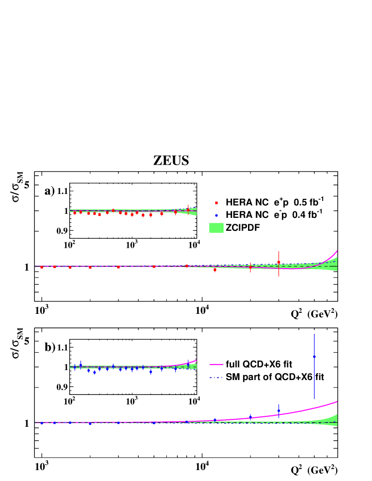
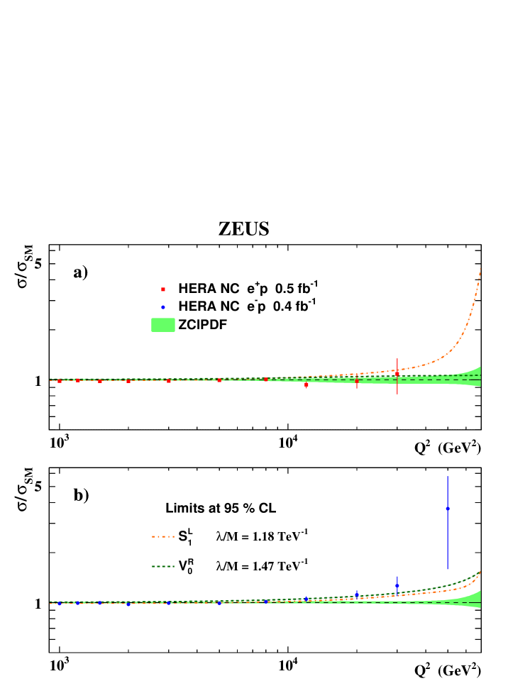
For six out of 13 considered CI scenarios and seven out of 14 heavy-LQ models, no significant improvement in description of the data was observed. The fits were consistent with , expected for a reduction of the number of degrees of freedom. The fitted coupling values for these models are consistent with zero. However, there are also four models (three CI and one444The improvement observed for the model is not considered, as it is obtained for an unphysical (negative) coupling value. LQ scenario), which result in an improved description of the data, with . The best description of the inclusive HERA data is obtained for the X6 model () and model (). The fit results for these models are compared with HERA NC DIS data in Fig. 1 and Fig. 2, respectively. Also indicated is the SM contribution to the NC DIS cross sections obtained from the QCD+CI fit.
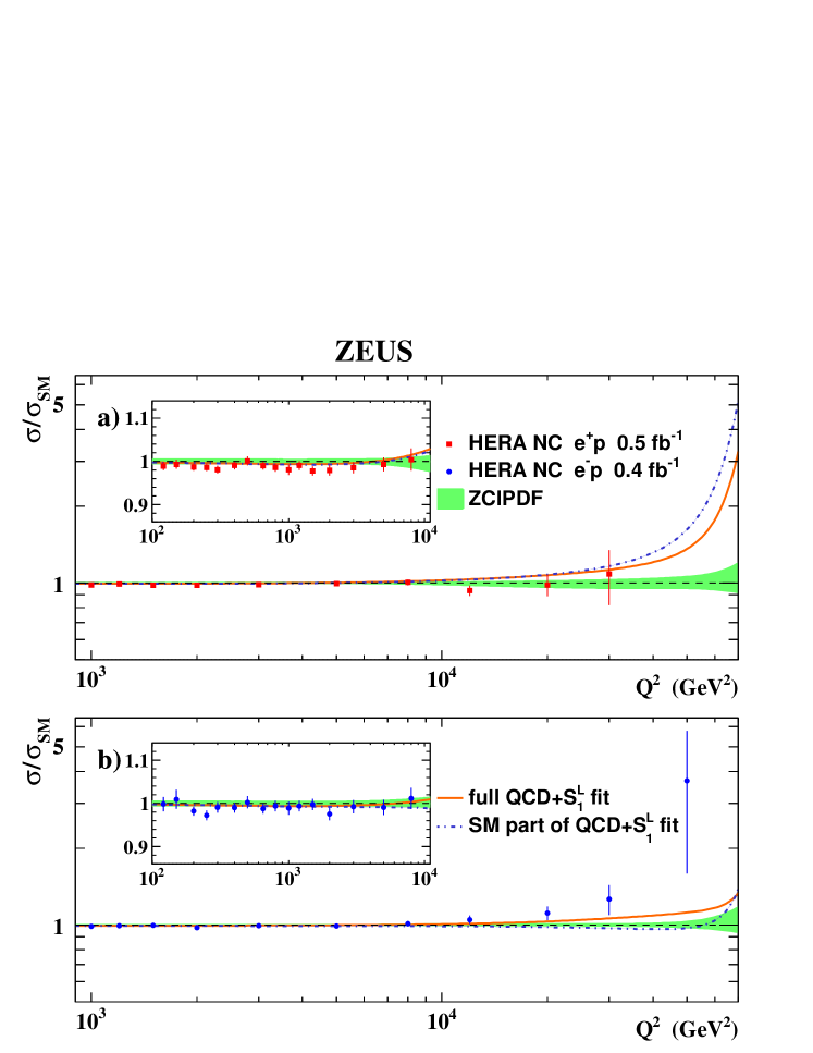
Figure 1 shows that, for the X6 model, the determination of the proton PDFs is affected very little by the CI contribution; the SM part of the NC DIS cross sections extracted from the QCD+CI fit agree with the nominal ZCIPDF fit within the quoted PDF uncertainties. The change in the predicted NC DIS cross section is dominated by the CI contribution. The situation is different for the heavy-LQ model shown in Fig. 2, where the description of the proton PDFs is significantly affected when the heavy-LQ contribution is taken into account in the fit. As a result, the cross-section prediction for NC DIS due to exchange increases at the highest values of , GeV2, by about a factor of two. The virtual leptoquark exchange contribution to the NC DIS cross section is much smaller than the change observed in the SM contribution. Moreover, it decreases the total cross section due to the negative interference with the SM part. The improvement in the description of the data for the heavy-LQ model is also due to the better agreement of the resulting predictions with the CC DIS data.
Table 1 also includes estimates of the modelling (and the resulting total) uncertainties on the fitted CI coupling values. For most of the models, the modelling uncertainties tend to be small, below the level of experimental uncertainties. However, they are significant for the three CI models, AA, X1 and X6, for which . Most important are the choice of the parameter (used to select the input data set for the fit) and the inclusion of the additional parameter [1] in the valence -quark density description. When the parameter is added to the ZCIPDF, it results in a . After the addition of the parameter, the improvement in due to the CI term is reduced for the AA, X1 and X6 models, and it is maximal for the VA model at .
For the LQ scenario, although modelling uncertainties are sizeable, see Table 2, they cannot explain the improvement in the description of the HERA data. The QCD+ fits result in for all considered model and parameterisation variations. The contribution to the predicted NC DIS cross section increases at the highest values. For scattering, the increase is expected at large values555This is due to an additional kinematic factor of multiplying the LL scattering amplitude for NC DIS.. A cross-check was also made using the bilog parameterisation [18]. While the overall description achieved with this quite different ansatz is much worse than the description achieved with the HERAPDF parameterisation, an term of similar strength was found.
4 Limit-setting precedure
The limits on the mass scales of the CI and heavy-LQ models were derived in a frequentist approach [24] using the technique of replicas.
4.1 Data set replicas
Replicas are sets of cross-section values, corresponding to the HERA inclusive data set that are generated by varying all cross sections randomly according to their known uncertainties. For the analysis presented here, multiple replica sets were used, each covering cross-section values on all points of the grid used in the QCD fit. For assumed true values of the CI coupling, , replica data sets were created by taking the reduced cross sections calculated from the nominal PDF fit (with CI coupling ) and scaling them with the cross-section ratio given by Eq. 5. This results in a set of cross-section values for the assumed true CI coupling . The values of were then varied randomly within the statistical and systematic uncertainties taken from the data, taking correlations of systematic uncertainties into account. All uncertainties were assumed to follow a Gaussian distribution666It was verified that using a Poisson probability distribution for producing replicas at high , where the event samples are small, and using the minimisation for these data did not change the results.. For each replica, the generated value of the cross section at the point , , was calculated as
| (7) |
where variables and represent random numbers from a normal distribution for each data point and for each source of correlated systematic uncertainty , respectively.
The approach adopted was to generate large sets of replicas and use them to test the hypothesis that the cross sections are consistent with the SM predictions or that they were modified by a fixed CI coupling according to Eq. 5. The fitted values from the replicas, , were used as a test statistics and compared to the corresponding value determined from a fit to the data.
To quantify the statistical consistency of the fit results with the SM expectations, the probability that an experiment assuming the validity of the SM (replicas generated with ) would produce a value of greater than (or less than) that obtained from the data was calculated:
| (8) |
where the probability was calculated from the distribution of values for a large set of generated SM replicas.
4.2 Constraining BSM scenarios
While for LQ models only positive values were considered, in the case of the CI scenarios, coupling limits were calculated separately for positive and negative values. The upper (lower) C.L. limit on the positive (negative) coupling, (), for a given scenario was determined as the value of for which 95% of the replicas produced a fitted coupling value, , larger (smaller) than that found in the data, , see Eq. 8. The corresponding mass-scale values ( and for CI scenarios or for LQ models) will be referred to as mass-scale limits. A similar procedure [7] was also used to calculate the expected limit values, which were defined by comparing replica fit results with instead of .
To take modelling uncertainties into account, the limit-calculation procedure was repeated for model or parameterisation variations resulting in the highest and the lowest values for each model. The weakest of the obtained coupling limits was taken as the result of the analysis and used to calculate the final mass-scale limits. This is clearly the most conservative approach, which is motivated by the difficulty in defining the underlying probability distribution for some of the considered modelling variations.
The expected limits are not sensitive to the modelling variations because these mainly affect the data fit results ( values) and the expected values do not depend on (replica fit results are compared to ). Therefore, these variations were not considered for the expected limits.
For each CI and LQ scenario, at least 3000 Monte Carlo replicas were generated and fitted for each value of . When using xFitter to perform replica fits, the inclusion of more models in the analysis was limited by the processing time. To facilitate efficient processing of replica data, a simplified fit method, based on the Taylor expansion of the cross-section predictions in terms of PDF parameters was developed, which reduced the processing time by almost two orders of magnitude [25].
5 Results
The probabilities (Eq. 8) calculated for the considered CI scenarios with the SM replica sets are presented in Table 4. The statistical approach based on Monte Carlo replicas confirms the observations described in Section 3.3, based on the values. For six CI models (LR, RL, VV, X2, X4 and X5), is above 20%, corresponding to less than a deviation from the nominal fit result (). For four models (LL, LR, VA and X3), the data fit results are reproduced by the SM replicas with 3–7% probability, corresponding to about a difference. However, for the three scenarios (AA, X1 and X6) with , is below 1%. This confirms that the differences between the HERA data and the SM predictions described by the additional CI contribution in the fit are unlikely to be due to statistical fluctuations only. As already discussed in Section 3.3, the effect can be explained to some extent by the modelling uncertainties, in particular by the deficiencies in the functional form used for the PDF parameterisation.
Also shown in Table 4 are the C.L. limits on the coupling values, and , for different CI models. Limits calculated without (exp) and with (exp+mod) model and parameterisation variations, as described above, are compared to the expected coupling limits in Fig. 3. Coupling limits can also be translated into limits on the compositeness scales for the considered CI scenarios, also included in Table 4.
For most of the CI scenarios considered, the interference term gives a significant contribution to the cross section and the sign of the CI coupling is well constrained in the fit. However, in the case of the VA model, the contribution from the interference term is much smaller than the direct CI contribution, which is proportional to the coupling squared. As a result, the model predictions are hardly sensitive to the coupling sign and the global minimum of the function is often observed for the “wrong” coupling sign (i.e. different from that of ). The limits on the CI coupling, calculated using the procedure described above, are therefore very weak ( and ). To solve this problem, limits for the VA model were calculated by restricting the fit range to negative or positive couplings, corresponding to the lower and upper coupling limit, respectively.
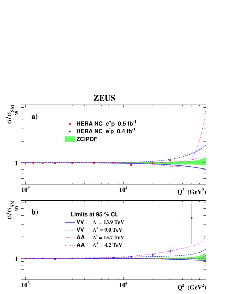
Compositeness-scale limits calculated taking modelling uncertainties into account range from 3.1 TeV for the X6 model () up to 17.9 TeV for the X3 model (). For the three models mentioned above (AA, X1 and X6), when only experimental uncertainties are considered, one sign of the CI coupling is excluded at C.L. and the limits for the coupling and compositeness scale are presented only for the other sign. The effect also persists when modelling uncertainties are taken into account for the X1 and X6 scenarios. In Fig. 4, the measured spectra of the HERA and data, relative to the SM predictions calculated using ZCIPDF, are compared with the expectations for the VV and AA contact-interaction models (as examples) which correspond to the compositeness limits described above.
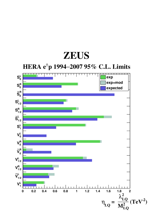
The LQ coupling values determined from the fit to the HERA inclusive data, , and the probabilities are summarised in Table 5 together with the coefficients describing the CI coupling structure of the considered LQ models. Also shown are the C.L. upper limits on the ratio of the Yukawa coupling to the leptoquark mass, . Limits calculated without (exp) and with (exp+mod) model and parameterisation variations are compared with the expected C.L. limits on in Fig. 5.
For the model, an improvement in the description of the HERA data can be obtained and the probability of reproducing the fit result with SM replicas, , is below 0.01%. For the model, the probability is 1.8%, which means that for both models is excluded at C.L. When modelling uncertainties are taken into account, the corresponding values increase, but are still below 5% for both models. A probability of less than 5% is also obtained for the and models.777Note that the is related to the model, corresponding to the same CI coupling structure, but with opposite sign. The fit results are therefore not independent. However, the fit gives unphysical (negative) coupling values so that both models are excluded at C.L.
Assuming the Yukawa coupling value, , the corresponding lower limits on the leptoquark mass vary between 0.66 TeV for the model and 16 TeV for the model. When modelling uncertainties are included, the limits vary between 0.60 TeV and 5.6 TeV. In Fig. 6, the measured spectra of the HERA and data, relative to the SM predictions calculated using ZCIPDF, are compared with the expectations for the and leptoquark models which correspond to the limits on the ratio of the leptoquark Yukawa coupling to the leptoquark mass shown in Fig. 5.
Two types of limits can be set on the considered BSM scenarios at the LHC. Direct searches for LQ pair-production result in limits for first-generation leptoquarks in the TeV range [26, 27]. These limits do not depend on the leptoquark Yukawa coupling and can not be directly compared to the presented HERA results. Independent limits on the ratio of the Yukawa coupling to the LQ mass, , as well as limits on the CI mass scales can be set from the analysis of the dilepton production in the Drell–Yan process. The diagram for this process corresponds to that describing NC DIS at HERA and the BSM contributions can be searched for in exactly the same CI framework.
A comparison of the present results with limits obtained by the ATLAS [28] and CMS [29] collaborations at the LHC, based on dilepton data collected at 13 TeV, is presented in Table 6. Only the four CI models shown were considered in the analyses of the LHC data. It is clear that, for these models, the statistical sensitivity of the LHC experiments is much higher than that of the HERA inclusive data. However, the systematic uncertainties resulting from the proton PDFs can be underestimated, as the possible bias in the parameterisation was not taken into account.
6 Conclusions
The HERA combined measurement of inclusive deep inelastic cross sections in neutral and charged current scattering has been used to search for possible deviations from the Standard Model predictions within the contact-interaction approximation. The procedure was based on a simultaneous fit of PDF parameters and the CI coupling. Limits on the CI couplings and probabilities for the SM predictions were obtained with Monte Carlo replicas. These were used to set limits on the CI compositeness scales, , and limits on the ratios of the leptoquark Yukawa coupling to the leptoquark mass, .
The addition of terms effective at high , such as those found in the CI and LQ models described above, reduces the tension between high- and low- data previously observed in the HERAPDF2.0 analysis. For the AA, VA, X1 and X6 models, the QCD+CI fits provide improved descriptions of the HERA inclusive data, corresponding to a difference from the SM predictions at the level of up to (SM probability of 0.3% for the X6 model). A similar effect is observed for the and leptoquark models, which give an improved description of the HERA inclusive data, corresponding to a difference from the SM predictions at a level of about and about , respectively. These deviations are unlikely to result from statistical fluctuations alone, but might be explicable by a combination of modelling uncertainties in the fitting procedure and statistical fluctuations. Since an unambiguous deviation from the SM cannot be established with the HERA data, limits for CI compositeness scales and LQ mass scales were set that are in the TeV range.
Acknowledgements
We appreciate the contributions to the construction, maintenance and operation of the ZEUS detector of many people who are not listed as authors. The HERA machine group and the DESY computing staff are especially acknowledged for their success in providing excellent operation of the collider and the data-analysis environment. We thank the DESY directorate for their strong support and encouragement.
10
References
- [1] H1 and ZEUS Collaborations, H. Abramowicz et al., Eur. Phys. J. C 75, 580 (2015)
- [2] V.N. Gribov and L.N. Lipatov, Sov. J. Nucl. Phys. 15, 438 (1972)
- [3] V.N. Gribov and L.N. Lipatov, Sov. J. Nucl. Phys. 15, 675 (1972)
- [4] L.N. Lipatov, Sov. J. Nucl. Phys. 20, 94 (1975)
- [5] Y.L. Dokshitzer, Sov. Phys. JETP 46, 641 (1977)
- [6] G. Altarelli and G. Parisi, Nucl. Phys. B 126, 298 (1977)
- [7] ZEUS Collaboration, H. Abramowicz et al., Phys. Lett. B 757, 468 (2016)
- [8] S. Chekanov et al., Phys. Lett. B 591, 23 (2004)
- [9] F.D. Aaron et al., Phys. Lett. B 705, 52 (2011)
- [10] F.D. Aaron et al., Phys. Lett. B 704, 388 (2011)
- [11] M. Tanabashi et al., Phys. Rev. D 98, 030001 (2018)
- [12] ZEUS Coll., S. Chekanov et al., Phys. Lett. B 591, 23 (2004)
- [13] J. Breitweg et al., Eur. Phys. J. C 14, 239 (2000)
-
[14]
W. Buchmüller, R. Rückl and D. Wyler,
Phys. Lett. B 191, 442 (1987).
Erratum in Phys. Lett. B 448, 320 (1999) - [15] A. Djouadi et al., Z. Phys. C 46, 679 (1990)
- [16] ZEUS Collaboration, H. Abramowicz et al., Phys. Rev. D 86, 012005 (2012)
- [17] J. Kalinowski et al., Z. Phys. C 74, 595 (1997)
- [18] V. Bertone et al., PoS DIS2017, 203 (2018)
- [19] S. Alekhin et al., Eur. Phys. J. C 75, 304 (2015)
- [20] A.D. Martin et al., Eur. Phys. J. C 63, 189 (2009)
- [21] P.M. Nadolsky et al., Phys. Rev. D 78, 013004 (2008)
- [22] ATLAS Collaboration, G. Aad et al., Phys. Rev. Lett. 109, 012001 (2012)
- [23] ATLAS Collaboration, M. Aaboud et al., Eur. Phys. J. C 77, 367 (2017)
- [24] R.D. Cousins, Am. J. Phys. 63, 398 (1995)
- [25] O. Turkot, K. Wichmann and A.F. Zarnecki, Simplified QCD fit method for BSM analysis of HERA data. arXiv:1606.06670 (unpublished)
- [26] ATLAS Collaboration, M. Aaboud et al., Searches for scalar leptoquarks and differential cross-section measurements in dilepton-dijet events in proton-proton collisions at a centre-of-mass energy of = 13 TeV with the ATLAS experiment. arXiv:1902.00377 (Submitted to JHEP), 2019
- [27] CMS Collaboration, A.M. Sirunyan et al., Phys. Rev. D99, 052002 (2019)
- [28] ATLAS Collaboration, M. Aaboud et al., JHEP 10, 182 (2017)
- [29] CMS Collaboration, A.M. Sirunyan et al., Search for contact interactions and large extra dimensions in the dilepton mass spectra from proton-proton collisions at 13 TeV. arXiv:1812.10443 (Accepted for publication in JHEP), 2018
| ZEUS | |||||||||
| HERA 1994–2007 data | |||||||||
| Coupling structure | Coupling fit results (TeV-2) | ||||||||
| Model | [ , | , | , | ] | |||||
| LL | [+1 , | 0, | 0, | 0] | 0.305 | 0.206 | 2.06 | ||
| RR | [ 0 , | 0, | 0, | +1] | 0.338 | 0.210 | 2.30 | ||
| LR | [ 0 , | +1, | 0, | 0] | 0.084 | 0.247 | 0.12 | ||
| RL | [ 0 , | 0, | +1, | 0] | 0.040 | 0.241 | 0.03 | ||
| VV | [+1 , | +1, | +1, | +1] | 0.041 | 0.061 | 0.45 | ||
| AA | [+1 , | , | , | +1] | 0.326 | 0.161 | 4.67 | ||
| VA | [+1, | , | +1, | ] | 0.594 | 0.225 | 1.21 | ||
| 0.676 | 0.200 | 3.25 | |||||||
| X1 | [+1 , | , | 0, | 0] | 0.682 | 0.267 | 5.52 | ||
| X2 | [+1 , | 0, | +1, | 0] | 0.089 | 0.121 | 0.52 | ||
| X3 | [+1 , | 0, | 0, | +1] | 0.158 | 0.108 | 2.09 | ||
| X4 | [ 0 , | +1, | +1, | 0] | 0.029 | 0.116 | 0.06 | ||
| X5 | [ 0 , | +1, | 0, | +1] | 0.079 | 0.123 | 0.41 | ||
| X6 | [ 0 , | 0, | +1, | ] | 0.786 | 0.274 | 6.01 | ||
| ZEUS | ||||||
|---|---|---|---|---|---|---|
| HERA 1994–2007 data | ||||||
| Model | Coupling Structure | Coupling fit results (TeV-2) | ||||
| 0.258 | 0.196 | 1.56 | ||||
| 0.533 | 0.331 | 2.53 | ||||
| 2.561 | 1.115 | 3.98 | ||||
| 0.054 | 0.341 | 0.02 | ||||
| 0.112 | 0.491 | 0.05 | ||||
| 0.464 | 1.371 | 0.10 | ||||
| 0.974 | 0.203 | 11.10 | ||||
| 0.325 | 0.116 | 6.17 | ||||
| 1.280 | 0.558 | 3.98 | ||||
| 0.267 | 0.165 | 2.53 | ||||
| 0.232 | 0.685 | 0.10 | ||||
| 0.056 | 0.246 | 0.05 | ||||
| 0.027 | 0.171 | 0.02 | ||||
| 0.029 | 0.077 | 0.14 | ||||
Variation Nominal Value Lower Limit Upper Limit [GeV2] 3.5 2.5 5.0 charm mass parameter [GeV] 1.47 1.41 1.53 beauty mass parameter [GeV] 4.5 4.25 4.75 sea strange fraction 0.4 0.3 0.5 starting scale [GeV2] 1.9 1.6 2.2
| ZEUS | ||||||||||||
| HERA 1994–2007 data | ||||||||||||
| 95% C.L. coupling limits (TeV-2) | 95% C.L. mass scale limits (TeV) | |||||||||||
| Model | Measured (exp) | Measured (exp+mod) | Expected | Measured (exp+mod) | Expected | |||||||
| (TeV-2) | (%) | |||||||||||
| LL | 0.305 | 7.0 | 0.033 | 0.610 | 0.077 | 0.616 | 0.367 | 0.319 | 12.8 | 4.5 | 5.9 | 6.3 |
| RR | 0.338 | 5.9 | 0.017 | 0.649 | 0.058 | 0.656 | 0.390 | 0.337 | 14.7 | 4.4 | 5.7 | 6.1 |
| LR | 0.084 | 34 | 0.514 | 0.250 | 0.565 | 0.413 | 0.388 | 0.313 | 4.7 | 5.5 | 5.7 | 6.3 |
| RL | 0.040 | 42 | 0.464 | 0.299 | 0.503 | 0.444 | 0.397 | 0.302 | 5.0 | 5.3 | 5.6 | 6.5 |
| VV | 0.041 | 25 | 0.058 | 0.135 | 0.065 | 0.155 | 0.101 | 0.097 | 13.9 | 9.0 | 11.2 | 11.4 |
| AA | 0.326 | 0.6 | 0.530 | 0.051 | 0.700 | 0.200 | 0.207 | 15.7 | 4.2 | 7.9 | 7.8 | |
| VA | 0.594 | 5.8 | 0.888 | 0.947 | 0.969 | 0.997 | 0.723 | 0.719 | 3.6 | 3.5 | 4.2 | 4.2 |
| 0.676 | 2.5 | |||||||||||
| X1 | 0.682 | 0.4 | 1.020 | 1.230 | 0.435 | 0.418 | 3.2 | 5.4 | 5.5 | |||
| X2 | 0.089 | 24 | 0.113 | 0.269 | 0.125 | 0.310 | 0.206 | 0.184 | 10.4 | 6.4 | 7.8 | 8.3 |
| X3 | 0.158 | 7.3 | 0.018 | 0.320 | 0.039 | 0.324 | 0.183 | 0.166 | 17.9 | 6.2 | 8.3 | 8.7 |
| X4 | 0.029 | 39 | 0.230 | 0.144 | 0.243 | 0.223 | 0.194 | 0.170 | 7.2 | 7.5 | 8.0 | 8.6 |
| X5 | 0.079 | 27 | 0.129 | 0.263 | 0.138 | 0.303 | 0.212 | 0.188 | 9.5 | 6.4 | 7.7 | 7.7 |
| X6 | 0.786 | 0.3 | 1.130 | 1.310 | 0.454 | 0.415 | 3.1 | 5.3 | 5.5 | |||
| ZEUS | ||||||
| HERA 1994–2007 data | ||||||
| 95% C.L. limits (TeV-1) | ||||||
| Model | Coupling Structure | Measured | Expected | |||
| (TeV-2) | (%) | (exp) | (exp+mod) | |||
| 0.258 | 9.0 | 0.25 | 0.28 | 0.56 | ||
| 0.533 | 5.5 | 1.02 | 1.03 | 0.72 | ||
| 2.561 | 1.8 | 1.71 | ||||
| 0.054 | 43 | 0.80 | 0.83 | 0.76 | ||
| 0.112 | 39 | 0.99 | 1.04 | 0.92 | ||
| 0.464 | 38 | 1.51 | 1.66 | 1.39 | ||
| 0.974 | 1.16 | 1.18 | 0.62 | |||
| 0.325 | 0.5 | 0.44 | ||||
| 1.280 | 1.8 | 1.44 | 1.47 | 0.99 | ||
| 0.267 | 5.5 | 0.06 | 0.18 | 0.53 | ||
| 0.232 | 38 | 1.12 | 1.19 | 1.29 | ||
| 0.056 | 39 | 0.55 | 0.67 | 0.57 | ||
| 0.027 | 43 | 0.47 | 0.59 | 0.49 | ||
| 0.029 | 32 | 0.39 | 0.41 | 0.25 | ||
| ZEUS | ||||||||||
|---|---|---|---|---|---|---|---|---|---|---|
| C.L. limits ( TeV) | ||||||||||
| Coupling structure | HERA | ATLAS | CMS | |||||||
| Model [ | , | , | , | ] | ||||||
| LL [ | +1, | 0, | 0, | 0 ] | 12.8 | 4.5 | 24 | 37 | 16.8 | 24.0 |
| RR [ | 0, | 0, | 0, | +1 ] | 14.7 | 4.4 | 26 | 33 | 16.9 | 23.8 |
| LR [ | 0, | +1, | 0, | 0 ] | 4.7 | 5.5 | 26 | 33 | 21.3 | 26.4 |
| RL [ | 0, | 0, | +1, | 0 ] | 5.0 | 5.3 | 26 | 33 | ||