Collaboration based Multi-Label Learning

Abstract

It is well-known that exploiting label correlations is crucially important to multi-label learning. Most of the existing approaches take label correlations as prior knowledge, which may not correctly characterize the real relationships among labels. Besides, label correlations are normally used to regularize the hypothesis space, while the final predictions are not explicitly correlated. In this paper, we suggest that for each individual label, the final prediction involves the collaboration between its own prediction and the predictions of other labels. Based on this assumption, we first propose a novel method to learn the label correlations via sparse reconstruction in the label space. Then, by seamlessly integrating the learned label correlations into model training, we propose a novel multi-label learning approach that aims to explicitly account for the correlated predictions of labels while training the desired model simultaneously. Extensive experimental results show that our approach outperforms the state-of-the-art counterparts.

Introduction

Multi-label learning deals with the problem where an instance can be associated with multiple labels simultaneously. Formally speaking, let $\mathcal{X}\in\mathbb{R}^{d}$ be $d$-dimensional feature space and $\mathcal{Y}=\{y_{1},y_{2},\cdots,y_{q}\}$ be the label space with $q$ labels. Given the multi-label training set $\mathcal{D}=\{\mathbf{x}_{i},\mathbf{y}_{i}\}_{i=1}^{n}$ where $\mathbf{x}_{i}\in\mathcal{X}$ is a feature vector and $\mathbf{y}_{i}\in\{-1,1\}^{q}$ is the label vector, the goal of multi-label learning is to learn a model $f:\mathbb{R}^{d}\rightarrow\{-1,1\}^{q}$, which maps from the space of feature vectors to the space of label vectors. As a learning framework that handles objects with multiple semantics, multi-label learning has been widely applied in many real-world applications, such as image annotation  (?), document categorization  (?), bioinformatics  (?), and information retrieval  (?).

The most straightforward multi-label learning approach (?) is to decompose the problem into a set of independent binary classification tasks, one for each label. Although this strategy is easy to implement, it may result in degraded performance, due to the ignorance of correlations among labels. To compensate for this deficiency, the exploitation of label correlations has been widely accepted as a key component of effective multi-label learning approaches (?; ?).

So far, many methods have been developed to improve the performance of multi-label learning by exploring various types of label correlations (?; ?; ?; ?; ?; ?). There has been increasing interest in exploiting the label correlations by taking the label correlation matrix as prior knowledge (?; ?; ?; ?). Concretely, these methods directly calculate the label correlation matrix by the similarity between label vectors using common similarity measures, and then incorporate the label correlation matrix into model training for further enhancing the predictions of multiple label assignments. However, the label correlations are simply obtained by common similarity measures, which may not be able to reflect complex relationships among labels. Besides, these methods exploit label correlations by manipulating the hypothesis space, while the final predictions are not explicitly correlated.

To address the above limitations, we make a key assumption that for each individual label, the final prediction involves the collaboration between its own prediction and the predictions of other labels. Based on this assumption, a novel multi-label learning approach named CAMEL, i.e., CollAboration based Multi-labEl Learning, is proposed. Different from most of the existing approaches that calculate the label correlation matrix simply by common similarity measures, CAMEL presents a novel method to learn such matrix and show that it is equivalent to sparse reconstruction in the label space. The learned label correlation matrix is capable of reflecting the collaborative relationships among labels regarding the final predictions. Subsequently, CAMEL seamlessly incorporates the learned label correlations into the desired multi-label predictive model. Specifically, label-independent embedding is introduced, which aims to fit the final predictions with the learned label correlations while guiding the estimation of the model parameters simultaneously. The effectiveness of CAMEL is clearly demonstrated by experimental results on a number of datasets.

Related Work

In recent years, many algorithms have been proposed to deal with multi-label learning tasks. In terms of the order of label correlations being considered, these approaches can be roughly categorized into three strategies (?; ?).

For the first-order strategy, the multi-label learning problem is tackled in a label-by-label manner where label correlations are ignored. Intuitively, one can easily decompose the multi-label learning problem into a series of independent binary classification problems (one for each label) (?). The second-order strategy takes into consideration pairwise relationships between labels, such as the ranking between relevant labels and irrelevant labels (?) or the interaction of paired labels (?). For the third-order strategy, high-order relationships among labels are considered. Following this strategy, numerous multi-label algorithms are proposed. For example, by modeling all other labels’ influences on each label, a shared subspace (?) is extracted for model training. By addressing connections among random subsets of labels, a chain of binary classifiers  (?) are sequentially trained.

Recently, there has been increasing interest in second-order approaches (?; ?; ?; ?) that take the label correlation matrix as prior knowledge for model training. These approaches normally directly calculate the label correlation matrix by the similarity between label vectors using common similarity measures, and then incorporate the label correlation matrix into model training for further enhancing the predictions of multiple label assignments. For instance, cosine similarity is widely used to calculate the label correlation matrix (?; ?; ?). Such label correlation matrix is further incorporated into a structured sparsity-inducing norm regularization (?) for regularizing the learning hypotheses, or performing joint label-specific feature selection and model training (?; ?). In addition, there are also some high-order approaches that exploit label correlations on the hypothesis space, while they do not rely on the label correlation matrix. For example, a boosting approach (?) is proposed to exploit label correlations with a hypothesis reuse mechanism.

Note that most of the existing approaches using label correlation matrix are second-order and focus on the hypothesis space. Such simple label correlations exploited in the hypothesis space may not correctly depict the real relationships among labels, and final predictions are not explicitly correlated. In the next section, a novel high-order approach with crafted label correlation matrix that focus on the label space will be introduced.

The CAMEL Approach

Following the notations used in Introduction, the training set can be alternatively represented by $\mathcal{D}=\{(\mathbf{X},\mathbf{Y})\}$ where $\mathbf{X}=[\mathbf{x}_{1},\mathbf{x}_{2},\cdots,\mathbf{x}_{n}]^{\top}\in\mathbb{R}^{n\times d}$ denotes the instance matrix, and $\mathbf{Y}=[\mathbf{y}_{1},\mathbf{y}_{2},\cdots,\mathbf{y}_{n}]^{\top}\in\mathbb{R}^{n\times q}$ denotes the label matrix. In addition, we denote by $\mathbf{Y}_{j}\in\mathbb{R}^{n}$ the $j$-th column vector of the matrix $\mathbf{Y}$ (versus $\mathbf{y}_{j}\in\mathbb{R}^{q}$ for the $j$-th row vector of $\mathbf{Y}$), and $\mathbf{Y}_{-j}=[\mathbf{Y}_{1},\cdots,\mathbf{Y}_{j-1},\mathbf{Y}_{j+1},\cdots,\mathbf{Y}_{q}]\in\mathbb{R}^{n\times(q-1)}$ represents the matrix that excludes the $j$-th column vector of $\mathbf{Y}$.

Label Correlation Learning

To characterize the collaborative relationships among labels regarding the final predictions, CAMEL works by learning a label correlation matrix $\mathbf{S}=[s_{ij}]_{q\times q}$ where $s_{ij}$ reflects the contribution of the $i$-label to the $j$-label. Guided by the assumption that for each individual label, the final prediction involves the collaboration between its own prediction and the predictions of other labels, we thus take the given label matrix as the final prediction, and propose to learn the label correlation matrix $\mathbf{S}$ in the following way:

$$\min_{s_{ij}}\left\|((1-\alpha)\mathbf{Y}_{j}+\alpha\sum_{i\neq j,i\in[q]}s_{ij}\mathbf{Y}_{i})-\mathbf{Y}_{j}\right\|_{2}^{2}$$ (1)

where $\alpha$ is the tradeoff parameter that controls the collaboration degree. In other words, $\alpha$ is used to balance the $j$-th label’s own prediction and the predictions of other labels. Since each label is normally correlated with only a few labels, the collaborative relationships between one label and other labels could be sparse. With a slight abuse of notation, we denote by $\mathbf{S}_{j}=[s_{1j},\cdots,s_{j-1,j},s_{j+1,j},\cdots,s_{qj}]^{\top}\in\mathbb{R}^{(q-1)}$ the $j$-th column vector of $\mathbf{S}$ excluding $s_{jj}$ ($s_{jj}=0$). Under canonical sparse representation, the coefficient vector $\mathbf{S}_{j}$ is learned by solving the following optimization problem:

$$\min_{\mathbf{S}_{j}}\left\|(1-\alpha)\mathbf{Y}_{j}+\alpha\mathbf{Y}_{-j}\mathbf{S}_{j}-\mathbf{Y}_{j}\right\|_{2}^{2}+\hat{\lambda}\left\|\mathbf{S}_{j}\right\|_{1}$$ (2)

where $\hat{\lambda}$ controls the sparsity of the coefficient vector $\mathbf{S}_{j}$. By properly rewriting the above problem and setting $\lambda=\hat{\lambda}/{\alpha}$, it is easy to derive the following equivalent optimization problem:

$$\min_{\mathbf{S}_{j}}\left\|\mathbf{Y}_{-j}\mathbf{S}_{j}-\mathbf{Y}_{j}\right\|_{2}^{2}+\lambda\left\|\mathbf{S}_{j}\right\|_{1}$$ (3)

Here, this problem aims to estimate the collaborative relationships between the $j$-th label and the other labels via sparse reconstruction. The first term corresponds to the linear reconstruction error via $\ell_{2}$ norm, and the second term controls the sparsity of the reconstruction coefficients by using $\ell_{1}$ norm. The relative importance of each term is balanced by the tradeoff parameter $\lambda$, which is empirically set to $\frac{1}{100}\left\|\mathbf{Y}_{j}^{\top}\mathbf{Y}_{-j}\right\|_{\infty}$ in the experiments. To solve problem (3), the popular Alternating Direction Method of Multiplier (ADMM) (?) is employed, and detailed information is given in Appendix A. After solving problem (3) for each label, the weight matrix $\mathbf{S}$ can be accordingly constructed with all diagonal elements set to 0. Note that for most of the existing second-order approaches using label correlation matrix (?; ?; ?; ?), only pairwise relationships are considered, and the relationships between one label and the other labels are separated. While for CAMEL, since the final prediction of each label is determined by all the predictions of other labels and itself, the relationships among all labels are exploited in a collaborative manner. Which means, the relationships between one label and the other labels are coordinated (influenced by each other). Therefore, CAMEL is a high-order approach.

Multi-Label Classifier Training

In this section, we propose a novel multi-label learning approach by seamlessly integrating the learned label correlations into the desired predictive model. Suppose the ordinary prediction matrix of $\mathbf{X}$ is denoted by $f(\mathbf{X})=[f_{1}(\mathbf{X}),f_{2}(\mathbf{X}),\cdots,f_{q}(\mathbf{X})]\in\mathbb{R}^{n\times q}$ where $f_{1}(\cdot),f_{2}(\cdot),\cdots,f_{q}(\cdot)$ denotes the individual label predictors respectively. In the ordinary setting, each label predictor is only in charge of a single label, while label correlations are fully lost. To absorb the learned label correlations into predictions, we reuse the assumption that for each individual label, the final prediction involves the collaboration between its own prediction and the predictions of other labels, and propose to compute the final prediction of the $j$-th label as follows:

$$(1-\alpha)f_{j}(\mathbf{X})+\alpha\sum_{i\neq j,i\in[q]}s_{ij}f_{i}(\mathbf{X})$$ (4)

where $\alpha$ is consistent with problem (1), which controls the collaboration degree of label predictions. By considering all the $q$ label predictions simultaneously, we thus obtain the following compact representation:

$$(1-\alpha)f(\mathbf{X})+\alpha f(\mathbf{X})\mathbf{S}=f(\mathbf{X})((1-\alpha)\mathbf{I}+\alpha\mathbf{S})$$ (5)

Here, the whole multi-label learning problem could be considered as two parallel subproblems, i.e., training the ordinary model and fitting the final predictions by the modeling outputs with label correlations. Thus, we propose to learn label-independent embedding denoted by $\mathbf{Z}\in\mathbb{R}^{n\times q}$, which works as a bridge between model training and prediction fitting. This brings several advantages: First, the two subproblems can be solved via alternation, which encourages the mutual adaption of model training and prediction fitting; Second, the relative importance of the two subproblems can be controlled by a tradeoff parameter; Third, closed-form solutions and kernel extension can be easily derived. Let $\mathbf{G}=(1-\alpha)\mathbf{I}+\alpha\mathbf{S}$, the proposed formulation is given as follows:

$$\min_{\mathbf{Z},f}\frac{1}{2}\left\|f(\mathbf{X})-\mathbf{Z}\right\|_{F}^{2}+\frac{\lambda_{1}}{2}\left\|\mathbf{Z}\mathbf{G}-\mathbf{Y}\right\|_{F}^{2}+\frac{\lambda_{2}}{2}\Omega(f)$$ (6)

where $\Omega(f)$ controls the complexity of the model $f$, $\lambda_{1}$ and $\lambda_{2}$ are the tradeoff parameters determining the relative importance of the above three terms. To instantiate the above formulation, we choose to train the widely-used model $f(\mathbf{X})=\phi(\mathbf{X})\mathbf{W}+\mathbf{1}\mathbf{b}^{\top}$ where $\mathbf{W}$ and $\mathbf{b}$ are the model parameters, $\mathbf{1}=[1,\cdots,1]^{\top}$ denotes the column vector with all elements equal to 1, and $\phi(\mathbf{\cdot})$ is a feature mapping that maps the feature space to some higher (maybe infinite) dimensional Hilbert space. For the regularization term to control the model complexity, we adopt the widely-used squared Frobenius norm, i.e., $\left\|\mathbf{W}\right\|_{F}^{2}$. To further facilitate a kernel extension for the general nonlinear case, we finally present the formulation as a constrained optimization problem:

$$\min_{\mathbf{W},\mathbf{Z},\mathbf{E},\mathbf{b}}\frac{1}{2}\left\|\mathbf{E}\right\|_{F}^{2}+\frac{\lambda_{1}}{2}\left\|\mathbf{Z}\mathbf{G}-\mathbf{Y}\right\|_{F}^{2}+\frac{\lambda_{2}}{2}\left\|\mathbf{W}\right\|_{F}^{2}$$ (7)

$$\text{s.t.}\quad\mathbf{Z}-\phi(\mathbf{X})\mathbf{W}-\mathbf{1}\mathbf{b}^{\top}=\mathbf{E}$$

Algorithm 1 The CAMEL Algorithm

0:  $\mathcal{D}$: the multi-label training set $\mathcal{D}=\{(\mathbf{X},\mathbf{Y})\}$$\alpha,\lambda_{1},\lambda_{2}$: the hyperparameters$\mathbf{x}$: the unseen test instance

0:  $\mathbf{y}$: the predicted label for the test instance $\mathbf{x}$

0:  

1:  learn the label correlation matrix $\mathbf{S}$ by solving problem (3) for each label via ADMM procedure;

2:  set $\mathbf{G}=(1-\alpha)\mathbf{I}+\alpha\mathbf{S}$;

3:  initialize $\mathbf{Z}=\mathbf{Y}$;

4:  construct the kernel matrix $\mathbf{K}=[\mathcal{K}(\mathbf{x}_{i},\mathbf{x}_{j})]_{n\times n}$ by Gaussian kernel function;

5:  repeat

6:     update $\mathbf{b}$ and $\mathbf{A}$ according to (9);

7:     update $\mathbf{T}=\frac{1}{\lambda_{2}}\mathbf{KA}+\mathbf{1}\mathbf{b}^{\top}$;

8:     update $\mathbf{Z}$ in terms of (11);

9:  until convergence.

10:  return the predicted label vector $\mathbf{y}$ according to (12).

Optimization

Problem (7) is convex with respect to $\mathbf{W}$ and $\mathbf{b}$ with $\mathbf{Z}$ fixed, and also convex with respect to $\mathbf{Z}$ with $\mathbf{W}$ and $\mathbf{b}$ fixed. Therefore, it is a biconvex problem (?), and can be solved by an alternating approach.

Updating $\mathbf{W}$ and $\mathbf{b}$ with $\mathbf{Z}$ fixed

With $\mathbf{Z}$ fixed, problem (7) reduces to

$$\min_{\mathbf{E},\mathbf{W},\mathbf{b}}\frac{1}{2}\left\|\mathbf{E}\right\|_{F}^{2}+\frac{\lambda_{2}}{2}\left\|\mathbf{W}\right\|_{F}^{2}$$ (8)

$$\text{s.t.}\quad\mathbf{Z}-\phi(\mathbf{X})\mathbf{W}-\mathbf{1}\mathbf{b}^{\top}=\mathbf{E}$$

By deriving the Lagrangian of the above constrained problem and setting the gradient with respect to $\mathbf{W}$ to 0, it is easy to show $\mathbf{W}=\frac{1}{\lambda_{2}}\phi(\mathbf{X})^{\top}\mathbf{A}$ where $\mathbf{A}=[a_{ij}]_{n\times q}$ is the matrix that stores the Lagrangian multipliers. Let $\mathbf{K}=\phi(\mathbf{X})\phi(\mathbf{X})^{\top}$ be the kernel matrix with its element $k_{ij}=\mathcal{K}(\mathbf{x}_{i},\mathbf{x}_{j})=\phi(\mathbf{x}_{i})^{\top}\phi(\mathbf{x}_{j})$, where $\mathcal{K}(\cdot,\cdot)$ represents the kernel function. For CAMEL, Gaussian kernel function $\mathcal{K}(\mathbf{x}_{i},\mathbf{x}_{j})=\exp(-\left\|\mathbf{x}_{i}-\mathbf{x}_{j}\right\|_{2}^{2}/(2\sigma^{2}))$ is employed with $\sigma$ set to the average Euclidean distance of all pairs of training instances. In this way, we choose to optimize with respect to $\mathbf{A}$ and $\mathbf{b}$ instead, and the close-form solutions are reported as follows:

$$\mathbf{b}^{\top} =\frac{\mathbf{1}^{\top}\mathbf{H}^{-1}\mathbf{Z}}{\mathbf{1}^{\top}\mathbf{H}^{-1}\mathbf{1}}$$ (9)

$$\mathbf{A} =\mathbf{H}^{-1}(\mathbf{Z}-\mathbf{1}\mathbf{b}^{\top})$$

where $\mathbf{H}=\frac{1}{\lambda_{2}}\mathbf{K}+\mathbf{I}$. The detailed information is provided in Appendix B.

Updating $\mathbf{Z}$ with $\mathbf{W}$ and $\mathbf{b}$ fixed

When $\mathbf{W}$ and $\mathbf{b}$ are fixed, the modeling output matrix $\mathbf{T}\in\mathbb{R}^{n\times q}$ is calculated by $\mathbf{T}=\phi(\mathbf{X})\mathbf{W}+\mathbf{1}\mathbf{b}^{\top}=\frac{1}{\lambda_{2}}\mathbf{K}\mathbf{A}+\mathbf{1}\mathbf{b}^{\top}$. By inserting $\mathbf{E}=\mathbf{Z}-\mathbf{T}$, problem (7) reduces to:

$$\min_{\mathbf{Z}}\frac{1}{2}\left\|\mathbf{Z}-\mathbf{T}\right\|_{F}^{2}+\frac{\lambda_{1}}{2}\left\|\mathbf{Z}\mathbf{G}-\mathbf{Y}\right\|_{F}^{2}$$ (10)

Setting the gradient with respect to $\mathbf{Z}$ to 0, we can obtain the following closed-form solution:

$$\mathbf{Z}=(\mathbf{T}+\lambda_{1}\mathbf{Y}\mathbf{G}^{\top})(\mathbf{I}+\lambda_{1}\mathbf{G}\mathbf{G}^{\top})^{-1}$$ (11)

Once the iterative process converges, the predicted label vector $\mathbf{y}\in\{-1,1\}^{l}$ of the test instance $\mathbf{x}$ is given as:

$$\mathbf{y}=\text{sign}(\mathbf{G}^{\top}(\sum_{i=1}^{m}\mathbf{a}_{i}\mathcal{K}(\mathbf{x},\mathbf{x}_{i})+\mathbf{b}))$$ (12)

The pseudo code of CAMEL is presented in Algorithm 1. Since the proposed formulation is biconvex, this alternating optimization process is guaranteed to converge (?).

Experiments

In this section, we conduct extensive experiments on various datasets to validate the effectiveness of CAMEL.

Experimental Setup

Datasets

For comprehensive performance evaluation, we collect sixteen benchmark multi-label datasets. For each dataset $\mathcal{S}$, we denote by $|\mathcal{S}|$, $dim(\mathcal{S})$, $L(\mathcal{S})$, $LCard(\mathcal{S})$, and $F(\mathcal{S})$ the number of examples, the number of features (dimensions), the number of distinct class labels, the average number of labels associated with each example, and feature type, respectively. Table 1 summarizes the detailed characteristics of these datasets, which are organized in ascending order of $|\mathcal{S}|$. According to $|\mathcal{S}|$, we further roughly divide these datasets into regular-size datasets ($|\mathcal{S}|<5000$) and large-size datasets ($|\mathcal{S}|\geq 5000$). For performance evaluation, 10-fold cross-validation is conducted on these datasets, where mean metric values with standard deviations are recorded.

Evaluation Metrics

For performance evaluation, we use seven widely-used evaluation metrics, including One-error, Hamming loss, Coverage, Ranking loss, Average precision, Macro-averaging F1, and Micro-averaging F1. Note that for all the employed multi-label evaluation metrics, their values vary within the interval [0,1]. In addition, for the last three metrics, the larger values indicate the better performance, and we use the symbol $\uparrow$ to present such positive logic. While for the first five metrics, the smaller values indicate the better performance, which is represented by $\downarrow$. More detailed information about these evaluation metrics can be found in (?).

Comparing Approaches

CAMEL is compared with three well-established and two state-of-the-art multi-label learning algorithms, including the first-order approach BR (?), the second-order approaches LLSF (?) and JFSC (?), and the high-order approaches ECC (?), and RAKEL (?). Here, LLSF and JFSC are the state-of-the-art counterparts using label correlation matrix.

BR, ECC, and RAKEL are implemented under the MULAN multi-label learning package (?) by using the logistic regression model as the base classifier. Furthermore, parameters suggested in the corresponding literatures are used, i.e., ECC: ensemble size 30; RAKEL: ensemble size $2q$ with $k=3$. For LLSF, parameters $\alpha,\beta$ are chosen from $\{2^{-10},2^{-9},\cdots,2^{10}\}$, and $\rho$ chosen from $\{0.1,1,10\}$. For JFSC, parameters $\alpha,\beta$, and $\gamma$ are chosen from $\{4^{-5},4^{-4},\cdots,4^{5}\}$, and $\eta$ is chosen from $\{0.1,1,10\}$. For the proposed approach CAMEL, $\lambda_{1}$ is empirically set to 1, $\lambda_{2}$ is chosen from $\{10^{-3},2\times 10^{-3},10^{-2},2\times 10^{-2},\cdots,10^{0}\}$, and $\alpha$ is chosen from $\{0,0.1,\cdots,1\}$. All of these parameters are decided by conducting 5-fold cross-validation on training set.

Table 1: Characteristics of the benchmark multi-label datasets.

Dataset	$|\mathcal{S}|$	$dim(\mathcal{S})$	$L(\mathcal{S})$	$LCard(\mathcal{S})$	$F(\mathcal{S})$
cal500	502	68	174	26.04	numeric
emotions	593	72	6	1.87	numeric
genbase	662	1185	27	1.25	nominal
medical	978	1449	45	1.25	nominal
enron	1702	1001	53	3.38	nominal
image	2000	294	5	1.24	numeric
scene	2407	294	5	1.07	numeric
yeast	2417	103	14	4.24	numeric
science	5000	743	40	1.45	numeric
arts	5000	462	26	1.64	numeric
business	5000	438	30	1.59	numeric
rcv1-s1	6000	944	101	2.88	nominal
rcv1-s2	6000	944	101	2.63	nominal
rcv1-s3	6000	944	101	2.61	nominal
rcv1-s4	6000	944	101	2.48	nominal
rcv1-s5	6000	944	101	2.64	nominal

Experimental Results

Table 2: Predictive performance of each algorithm (mean$\pm$std. deviation) on the regular-scale datasets.

Comparing algorithms	One-error$\downarrow$
	cal500	emotions	genbase	medical	enron	image	scene	yeast
CAMEL	0.129$\pm$0.053	0.292$\pm$0.052	0.001$\pm$0.001	0.110$\pm$0.021	0.207$\pm$0.038	0.242$\pm$0.033	0.175$\pm$0.027	0.218$\pm$0.027
BR	0.893$\pm$0.038	0.284$\pm$0.077	0.017$\pm$0.016	0.322$\pm$0.055	0.646$\pm$0.023	0.387$\pm$0.027	0.361$\pm$0.036	0.244$\pm$0.028
ECC	0.295$\pm$0.036	0.296$\pm$0.074	0.010$\pm$0.013	0.156$\pm$0.037	0.421$\pm$0.034	0.406$\pm$0.023	0.306$\pm$0.020	0.238$\pm$0.030
RAKEL	0.634$\pm$0.039	0.300$\pm$0.070	0.009$\pm$0.007	0.243$\pm$0.055	0.532$\pm$0.007	0.402$\pm$0.024	0.280$\pm$0.031	0.244$\pm$0.027
LLSF	0.138$\pm$0.050	0.412$\pm$0.051	0.002$\pm$0.005	0.120$\pm$0.020	0.250$\pm$0.042	0.327$\pm$0.030	0.259$\pm$0.020	0.394$\pm$0.029
JFSC	0.116$\pm$0.051	0.438$\pm$0.086	0.002$\pm$0.005	0.128$\pm$0.024	0.278$\pm$0.041	0.346$\pm$0.023	0.266$\pm$0.022	0.242$\pm$0.021
Comparing algorithms	Hamming loss$\downarrow$
	cal500	emotions	genbase	medical	enron	image	scene	yeast
CAMEL	0.136$\pm$0.005	0.203$\pm$0.021	0.001$\pm$0.001	0.011$\pm$0.001	0.045$\pm$0.003	0.144$\pm$0.012	0.072$\pm$0.009	0.190$\pm$0.005
BR	0.189$\pm$0.005	0.216$\pm$0.028	0.002$\pm$0.002	0.026$\pm$0.003	0.111$\pm$0.006	0.210$\pm$0.014	0.139$\pm$0.009	0.205$\pm$0.007
ECC	0.154$\pm$0.005	0.214$\pm$0.027	0.009$\pm$0.004	0.011$\pm$0.002	0.067$\pm$0.002	0.210$\pm$0.016	0.112$\pm$0.006	0.204$\pm$0.010
RAKEL	0.195$\pm$0.004	0.238$\pm$0.025	0.002$\pm$0.001	0.020$\pm$0.002	0.092$\pm$0.004	0.223$\pm$0.013	0.139$\pm$0.008	0.224$\pm$0.009
LLSF	0.138$\pm$0.006	0.267$\pm$0.022	0.001$\pm$0.001	0.010$\pm$0.002	0.048$\pm$0.002	0.180$\pm$0.010	0.109$\pm$0.003	0.278$\pm$0.009
JFSC	0.191$\pm$0.004	0.295$\pm$0.019	0.001$\pm$0.001	0.010$\pm$0.001	0.051$\pm$0.003	0.188$\pm$0.012	0.110$\pm$0.007	0.206$\pm$0.006
Comparing algorithms	Coverage$\downarrow$
	cal500	emotions	genbase	medical	enron	image	scene	yeast
CAMEL	0.752$\pm$0.019	0.312$\pm$0.031	0.012$\pm$0.005	0.028$\pm$0.012	0.239$\pm$0.028	0.156$\pm$0.016	0.062$\pm$0.006	0.446$\pm$0.010
BR	0.786$\pm$0.015	0.319$\pm$0.026	0.014$\pm$0.006	0.113$\pm$0.030	0.580$\pm$0.023	0.216$\pm$0.018	0.168$\pm$0.015	0.463$\pm$0.011
ECC	0.796$\pm$0.019	0.310$\pm$0.029	0.013$\pm$0.003	0.034$\pm$0.012	0.291$\pm$0.020	0.233$\pm$0.022	0.135$\pm$0.010	0.460$\pm$0.010
RAKEL	0.962$\pm$0.016	0.362$\pm$0.027	0.014$\pm$0.005	0.095$\pm$0.018	0.513$\pm$0.019	0.253$\pm$0.017	0.169$\pm$0.013	0.544$\pm$0.013
LLSF	0.778$\pm$0.025	0.362$\pm$0.032	0.021$\pm$0.006	0.031$\pm$0.014	0.283$\pm$0.023	0.192$\pm$0.007	0.092$\pm$0.006	0.601$\pm$0.020
JFSC	0.730$\pm$0.026	0.392$\pm$0.046	0.014$\pm$0.007	0.030$\pm$0.012	0.314$\pm$0.024	0.200$\pm$0.009	0.102$\pm$0.007	0.455$\pm$0.011
Comparing algorithms	Ranking loss$\downarrow$
	cal500	emotions	genbase	medical	enron	image	scene	yeast
CAMEL	0.177$\pm$0.009	0.180$\pm$0.032	0.001$\pm$0.001	0.016$\pm$0.008	0.079 $\pm$0.028	0.128$\pm$0.013	0.058$\pm$0.005	0.162$\pm$0.007
BR	0.233$\pm$0.007	0.182$\pm$0.030	0.003$\pm$0.004	0.091$\pm$0.027	0.304$\pm$0.014	0.204$\pm$0.017	0.151$\pm$0.015	0.176$\pm$0.008
ECC	0.219$\pm$0.007	0.172$\pm$0.031	0.002$\pm$0.002	0.022$\pm$0.010	0.118$\pm$0.008	0.225$\pm$0.023	0.117$\pm$0.010	0.179$\pm$0.009
RAKEL	0.366$\pm$0.008	0.225$\pm$0.029	0.002$\pm$0.001	0.073$\pm$0.018	0.244$\pm$0.017	0.221$\pm$0.018	0.131$\pm$0.014	0.240$\pm$0.009
LLSF	0.184$\pm$0.012	0.245$\pm$0.033	0.002$\pm$0.003	0.019$\pm$0.010	0.107$\pm$0.009	0.174$\pm$0.006	0.093$\pm$0.005	0.346$\pm$0.017
JFSC	0.188$\pm$0.010	0.271$\pm$0.041	0.003$\pm$0.003	0.017$\pm$0.008	0.118$\pm$0.013	0.183$\pm$0.007	0.105$\pm$0.007	0.179$\pm$0.009
Comparing algorithms	Average precision$\uparrow$
	cal500	emotions	genbase	medical	enron	image	scene	yeast
CAMEL	0.515$\pm$0.018	0.788$\pm$0.035	0.997$\pm$0.003	0.917$\pm$0.017	0.718$\pm$0.025	0.843$\pm$0.018	0.897$\pm$0.012	0.775$\pm$0.013
BR	0.345$\pm$0.018	0.783$\pm$0.040	0.988$\pm$0.008	0.750$\pm$0.036	0.388$\pm$0.016	0.753$\pm$0.016	0.771$\pm$0.021	0.754$\pm$0.013
ECC	0.442$\pm$0.014	0.789$\pm$0.036	0.991$\pm$0.008	0.884$\pm$0.023	0.557$\pm$0.015	0.738$\pm$0.020	0.811$\pm$0.012	0.756$\pm$0.014
RAKEL	0.329$\pm$0.016	0.763$\pm$0.039	0.993$\pm$0.006	0.800$\pm$0.032	0.456$\pm$0.019	0.735$\pm$0.017	0.804$\pm$0.022	0.720$\pm$0.014
LLSF	0.507$\pm$0.021	0.716$\pm$0.035	0.997$\pm$0.005	0.912$\pm$0.015	0.682$\pm$0.028	0.790$\pm$0.014	0.843$\pm$0.008	0.601$\pm$0.015
JFSC	0.492$\pm$0.020	0.691$\pm$0.040	0.997$\pm$0.004	0.908$\pm$0.016	0.655$\pm$0.025	0.779$\pm$0.011	0.835$\pm$0.010	0.746$\pm$0.012
Comparing algorithms	Macro-averaging F1$\uparrow$
	cal500	emotions	genbase	medical	enron	image	scene	yeast
CAMEL	0.180$\pm$0.032	0.625$\pm$0.052	0.971$\pm$0.030	0.779$\pm$0.043	0.325$\pm$0.044	0.660$\pm$0.030	0.787$\pm$0.023	0.411$\pm$0.018
BR	0.167$\pm$0.019	0.620$\pm$0.044	0.951$\pm$0.029	0.640$\pm$0.060	0.236$\pm$0.016	0.553$\pm$0.027	0.623$\pm$0.026	0.391$\pm$0.021
ECC	0.236$\pm$0.027	0.622$\pm$0.043	0.928$\pm$0.037	0.755$\pm$0.054	0.303$\pm$0.030	0.540$\pm$0.030	0.662$\pm$0.026	0.395$\pm$0.015
RAKEL	0.187$\pm$0.020	0.614$\pm$0.044	0.958$\pm$0.030	0.689$\pm$0.051	0.256$\pm$0.017	0.540$\pm$0.028	0.644$\pm$0.024	0.381$\pm$0.020
LLSF	0.180$\pm$0.031	0.615$\pm$0.056	0.971$\pm$0.031	0.769$\pm$0.057	0.292$\pm$0.043	0.554$\pm$0.031	0.615$\pm$0.007	0.235$\pm$0.016
JFSC	0.239$\pm$0.031	0.345$\pm$0.023	0.971$\pm$0.031	0.772$\pm$0.043	0.339$\pm$0.048	0.559$\pm$0.035	0.705$\pm$0.019	0.300$\pm$0.007
Comparing algorithms	Micro-averaging F1$\uparrow$
	cal500	emotions	genbase	medical	enron	image	scene	yeast
CAMEL	0.337$\pm$0.017	0.649$\pm$0.041	0.988$\pm$0.012	0.835$\pm$0.019	0.580$\pm$0.023	0.659$\pm$0.031	0.780$\pm$0.026	0.655$\pm$0.010
BR	0.339$\pm$0.016	0.639$\pm$0.050	0.978$\pm$0.014	0.611$\pm$0.032	0.359$\pm$0.015	0.558$\pm$0.028	0.619$\pm$0.023	0.633$\pm$0.013
ECC	0.364$\pm$0.015	0.642$\pm$0.046	0.907$\pm$0.035	0.796$\pm$0.023	0.452$\pm$0.015	0.541$\pm$0.030	0.653$\pm$0.023	0.643$\pm$0.017
RAKEL	0.351$\pm$0.018	0.629$\pm$0.049	0.983$\pm$0.011	0.678$\pm$0.042	0.392$\pm$0.014	0.541$\pm$0.031	0.629$\pm$0.026	0.632$\pm$0.016
LLSF	0.325$\pm$0.015	0.637$\pm$0.049	0.992$\pm$0.003	0.823$\pm$0.027	0.534$\pm$0.025	0.557$\pm$0.032	0.618$\pm$0.008	0.280$\pm$0.018
JFSC	0.473$\pm$0.013	0.406$\pm$0.022	0.995$\pm$0.006	0.818$\pm$0.018	0.555$\pm$0.026	0.565$\pm$0.033	0.695$\pm$0.022	0.609$\pm$0.012

Table 3: Predictive performance of each algorithm (mean$\pm$std. deviation) on the large-scale datasets.

Comparing algorithms	One-error$\downarrow$
	science	arts	rcv1-s1	rcv1-s2	rcv1-s3	rcv1-s4	rcv1-s5	business
CAMEL	0.457$\pm$0.021	0.462$\pm$0.024	0.404$\pm$0.019	0.403$\pm$0.018	0.413$\pm$0.019	0.331$\pm$0.016	0.404$\pm$0.010	0.101$\pm$0.009
BR	0.760$\pm$0.015	0.642$\pm$0.022	0.742$\pm$0.019	0.723$\pm$0.024	0.718$\pm$0.021	0.662$\pm$0.021	0.715$\pm$0.015	0.417$\pm$0.016
ECC	0.574$\pm$0.022	0.526$\pm$0.023	0.471$\pm$0.020	0.441$\pm$0.021	0.448$\pm$0.021	0.378$\pm$0.019	0.425$\pm$0.016	0.153$\pm$0.008
RAKEL	0.623$\pm$0.014	0.543$\pm$0.024	0.613$\pm$0.019	0.592$\pm$0.022	0.578$\pm$0.020	0.552$\pm$0.020	0.575$\pm$0.014	0.201$\pm$0.009
LLSF	0.486$\pm$0.013	0.454$\pm$0.027	0.409$\pm$0.015	0.406$\pm$0.016	0.415$\pm$0.021	0.333$\pm$0.016	0.399$\pm$0.018	0.122$\pm$0.016
JFSC	0.489$\pm$0.027	0.447$\pm$0.027	0.418$\pm$0.016	0.407$\pm$0.014	0.418$\pm$0.025	0.337$\pm$0.015	0.407$\pm$0.023	0.122$\pm$0.019
Comparing algorithms	Hamming loss$\downarrow$
	science	arts	rcv1-s1	rcv1-s2	rcv1-s3	rcv1-s4	rcv1-s5	business
CAMEL	0.030$\pm$0.001	0.055$\pm$0.002	0.026$\pm$0.008	0.023$\pm$0.001	0.023$\pm$0.001	0.018$\pm$0.001	0.022$\pm$0.001	0.024$\pm$0.001
BR	0.072$\pm$0.002	0.079$\pm$0.003	0.056$\pm$0.001	0.053$\pm$0.001	0.053$\pm$0.001	0.041$\pm$0.001	0.051$\pm$0.002	0.049$\pm$0.001
ECC	0.036$\pm$0.002	0.063$\pm$0.002	0.028$\pm$0.001	0.024$\pm$0.001	0.024$\pm$0.001	0.019$\pm$0.001	0.024$\pm$0.001	0.030$\pm$0.001
RAKEL	0.042$\pm$0.002	0.075$\pm$0.002	0.046$\pm$0.001	0.039$\pm$0.001	0.035$\pm$0.001	0.035$\pm$0.001	0.036$\pm$0.003	0.035$\pm$0.002
LLSF	0.036$\pm$0.002	0.054$\pm$0.002	0.027$\pm$0.001	0.025$\pm$0.001	0.025$\pm$0.001	0.019$\pm$0.001	0.023$\pm$0.001	0.048$\pm$0.007
JFSC	0.035$\pm$0.002	0.057$\pm$0.002	0.029$\pm$0.001	0.025$\pm$0.001	0.025$\pm$0.001	0.019$\pm$0.001	0.025$\pm$0.001	0.027$\pm$0.002
Comparing algorithms	Coverage$\downarrow$
	science	arts	rcv1-s1	rcv1-s2	rcv1-s3	rcv1-s4	rcv1-s5	business
CAMEL	0.189$\pm$0.010	0.205$\pm$0.009	0.151$\pm$0.008	0.142$\pm$0.012	0.131$\pm$0.006	0.143$\pm$0.003	0.132$\pm$0.005	0.082$\pm$0.006
BR	0.303$\pm$0.011	0.204$\pm$0.009	0.393$\pm$0.011	0.341$\pm$0.013	0.351$\pm$0.018	0.294$\pm$0.015	0.336$\pm$0.013	0.141$\pm$0.002
ECC	0.196$\pm$0.009	0.229$\pm$0.009	0.166$\pm$0.011	0.154$\pm$0.007	0.154$\pm$0.008	0.108$\pm$0.003	0.145$\pm$0.001	0.104$\pm$0.001
RAKEL	0.209$\pm$0.012	0.214$\pm$0.008	0.273$\pm$0.011	0.329$\pm$0.012	0.293$\pm$0.017	0.273$\pm$0.012	0.246$\pm$0.012	0.107$\pm$0.003
LLSF	0.197$\pm$0.014	0.195$\pm$0.011	0.141$\pm$0.009	0.146$\pm$0.008	0.133$\pm$0.008	0.109$\pm$0.006	0.133$\pm$0.006	0.086$\pm$0.013
JFSC	0.196$\pm$0.011	0.233$\pm$0.018	0.140$\pm$0.006	0.143$\pm$0.009	0.136$\pm$0.010	0.106$\pm$0.005	0.139$\pm$0.006	0.086$\pm$0.011
Comparing algorithms	Ranking loss$\downarrow$
	science	arts	rcv1-s1	rcv1-s2	rcv1-s3	rcv1-s4	rcv1-s5	business
CAMEL	0.139$\pm$0.007	0.135$\pm$0.008	0.058$\pm$0.003	0.077$\pm$0.005	0.047$\pm$0.003	0.057$\pm$0.002	0.073$\pm$0.002	0.040$\pm$0.004
BR	0.245$\pm$0.009	0.145$\pm$0.006	0.197$\pm$0.006	0.190$\pm$0.008	0.198$\pm$0.010	0.173$\pm$0.009	0.181$\pm$0.006	0.088$\pm$0.006
ECC	0.151$\pm$0.006	0.164$\pm$0.007	0.074$\pm$0.005	0.069$\pm$0.003	0.070$\pm$0.002	0.047$\pm$0.004	0.063$\pm$0.003	0.055$\pm$0.002
RAKEL	0.195$\pm$0.007	0.156$\pm$0.008	0.183$\pm$0.006	0.153$\pm$0.008	0.178$\pm$0.010	0.112$\pm$0.009	0.123$\pm$0.006	0.067$\pm$0.005
LLSF	0.149$\pm$0.009	0.141$\pm$0.009	0.060$\pm$0.003	0.060$\pm$0.004	0.048$\pm$0.003	0.034$\pm$0.003	0.045$\pm$0.003	0.045$\pm$0.009
JFSC	0.147$\pm$0.008	0.159$\pm$0.009	0.061$\pm$0.003	0.062$\pm$0.006	0.061$\pm$0.004	0.047$\pm$0.003	0.060$\pm$0.003	0.045$\pm$0.008
Comparing algorithms	Average precision$\uparrow$
	science	arts	rcv1-s1	rcv1-s2	rcv1-s3	rcv1-s4	rcv1-s5	business
CAMEL	0.624$\pm$0.016	0.607$\pm$0.018	0.615$\pm$0.009	0.644$\pm$0.012	0.635$\pm$0.010	0.717$\pm$0.008	0.626$\pm$0.009	0.891$\pm$0.009
BR	0.383$\pm$0.011	0.514$\pm$0.013	0.353$\pm$0.011	0.382$\pm$0.015	0.382$\pm$0.015	0.443$\pm$0.013	0.390$\pm$0.009	0.709$\pm$0.008
ECC	0.516$\pm$0.020	0.553$\pm$0.018	0.545$\pm$0.016	0.587$\pm$0.015	0.585$\pm$0.016	0.677$\pm$0.017	0.600$\pm$0.009	0.844$\pm$0.005
RAKEL	0.487$\pm$0.012	0.526$\pm$0.015	0.424$\pm$0.012	0.489$\pm$0.016	0.459$\pm$0.014	0.479$\pm$0.012	0.432$\pm$0.009	0.858$\pm$0.007
LLSF	0.594$\pm$0.021	0.631$\pm$0.016	0.627$\pm$0.009	0.637$\pm$0.008	0.632$\pm$0.013	0.714$\pm$0.010	0.625$\pm$0.013	0.867$\pm$0.013
JFSC	0.595$\pm$0.020	0.621$\pm$0.020	0.606$\pm$0.008	0.630$\pm$0.009	0.624$\pm$0.014	0.700$\pm$0.012	0.624$\pm$0.013	0.874$\pm$0.018
Comparing algorithms	Macro-averaging F1$\uparrow$
	science	arts	rcv1-s1	rcv1-s2	rcv1-s3	rcv1-s4	rcv1-s5	business
CAMEL	0.310$\pm$0.038	0.312$\pm$0.029	0.250$\pm$0.023	0.258$\pm$0.022	0.247$\pm$0.025	0.340$\pm$0.031	0.253$\pm$0.016	0.326$\pm$0.046
BR	0.215$\pm$0.048	0.257$\pm$0.020	0.232$\pm$0.018	0.210$\pm$0.017	0.221$\pm$0.019	0.313$\pm$0.016	0.236$\pm$0.019	0.249$\pm$0.017
ECC	0.285$\pm$0.024	0.282$\pm$0.021	0.271$\pm$0.023	0.257$\pm$0.022	0.266$\pm$0.012	0.334$\pm$0.018	0.285$\pm$0.014	0.326$\pm$0.032
RAKEL	0.267$\pm$0.028	0.275$\pm$0.019	0.266$\pm$0.019	0.237$\pm$0.023	0.243$\pm$0.017	0.322$\pm$0.017	0.255$\pm$0.018	0.307$\pm$0.024
LLSF	0.312$\pm$0.038	0.219$\pm$0.032	0.261$\pm$0.022	0.257$\pm$0.025	0.270$\pm$0.027	0.334$\pm$0.031	0.217$\pm$0.018	0.325$\pm$0.028
JFSC	0.308$\pm$0.039	0.305$\pm$0.032	0.308$\pm$0.026	0.249$\pm$0.019	0.258$\pm$0.024	0.337$\pm$0.032	0.254$\pm$0.019	0.318$\pm$0.036
Comparing algorithms	Micro-averaging F1$\uparrow$
	science	arts	rcv1-s1	rcv1-s2	rcv1-s3	rcv1-s4	rcv1-s5	business
CAMEL	0.428$\pm$0.018	0.415$\pm$0.015	0.401$\pm$0.015	0.437$\pm$0.017	0.431$\pm$0.025	0.491$\pm$0.017	0.441$\pm$0.015	0.746$\pm$0.011
BR	0.277$\pm$0.013	0.349$\pm$0.018	0.301$\pm$0.009	0.310$\pm$0.009	0.307$\pm$0.013	0.356$\pm$0.009	0.321$\pm$0.009	0.595$\pm$0.003
ECC	0.343$\pm$0.028	0.377$\pm$0.018	0.385$\pm$0.016	0.410$\pm$0.022	0.414$\pm$0.013	0.482$\pm$0.024	0.440$\pm$0.011	0.690$\pm$0.007
RAKEL	0.337$\pm$0.014	0.368$\pm$0.017	0.341$\pm$0.010	0.337$\pm$0.008	0.335$\pm$0.014	0.369$\pm$0.008	0.350$\pm$0.008	0.701$\pm$0.014
LLSF	0.446$\pm$0.025	0.368$\pm$0.018	0.463$\pm$0.016	0.432$\pm$0.018	0.428$\pm$0.023	0.478$\pm$0.017	0.438$\pm$0.019	0.693$\pm$0.035
JFSC	0.449$\pm$0.026	0.442$\pm$0.017	0.456$\pm$0.008	0.422$\pm$0.011	0.424$\pm$0.012	0.482$\pm$0.013	0.438$\pm$0.011	0.712$\pm$0.021

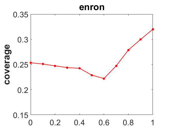
(a) $\alpha$

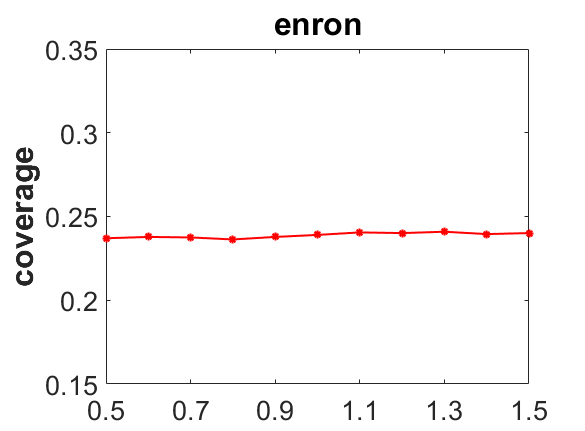
(b) $\lambda_{1}$

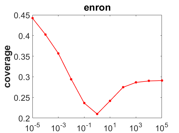
(c) $\lambda_{2}$

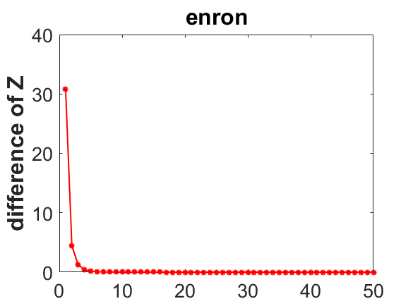
(d) Convergence Curve

Figure 1: Parameter sensitivity and convergence analysis of CAMEL on the enron dataset.

Table 2 and 3 report the detailed experimental results on the regular-scale and large-scale datasets respectively, where the best performance among all the algorithms is shown in boldface. From the two result tables, we can see that CAMEL outperforms other comparing algorithms in most cases. Specifically, on the regular-size datasets (Table 2), across all the evaluation metrics, CAMEL ranks first in 80.4% (45/56) cases, and on the large-scale datasets (Table 3), across all the evaluation metrics, CAMEL ranks first in 69.6% (39/56) cases. Compared with the three well-established algorithms BR, ECC, and RAKEL, CAMEL introduces a new type of label correlations, i.e., collaborative relationships among labels, and achieves superior performance in 93.8% (315/336) cases. Compared with the two state-of-the-art algorithms LLSF and JFSC, instead of employing simple similarity measures to regularize the hypothesis space, CAMEL introduces a novel method to learn label correlations for explicitly correlating the final predictions, and achieves superior performance in 80.4% (180/224) cases. These comparative results clearly demonstrate the effectiveness of the collaboration based multi-label learning approach.

Sensitivity Analysis

In this section, we first investigate the sensitivity of CAMEL with respect to the two tradeoff parameters $\lambda_{1}$ and $\lambda_{2}$, and the parameter $\alpha$ that controls the degree of collaboration, then illustrate the convergence of CAMEL. Due to page limit, we only report the experimental results on the enron dataset using the Coverage ($\downarrow$) metric. Concretely, we study the performance of CAMEL when we vary one parameter while keeping other parameters fixed at their best setting. Figure 1(a), 1(b), and 1(c) show the sensitivity curve of CAMEL with respect to $\alpha$, $\lambda_{1}$, and $\lambda_{2}$ respectively. It can be seen that $\alpha$ and $\lambda_{2}$ have an important influence on the final performance, because $\alpha$ and $\lambda_{2}$ control the collaboration degree and the model complexity. Figure 1(d) illustrates the convergence of CAMEL by using the difference of the optimization variable $\mathbf{Z}$ between two successive iterations, i.e., $\Delta\mathbf{Z}=\left\|\mathbf{Z}^{(t)}-\mathbf{Z}^{(t-1)}\right\|_{F}$. From Figure 1(d), we can observe that $\Delta\mathbf{Z}$ quickly decreases to 0 within a few number of iterations. Hence the convergence of CAMEL is demonstrated.

Conclusion

In this paper, we make a key assumption for multi-label learning that for each individual label, the final prediction involves the collaboration between its own prediction and the predictions of other labels. Guided by this assumption, we propose a novel method to learn the high-order label correlations via sparse reconstruction in the label space. Besides, by seamlessly integrating the learned label correlations into model training, we propose a novel multi-label learning approach that aims to explicitly account for the correlated predictions of labels while training the desired model simultaneously. Extensive experimental results show that our approach outperforms the state-of-the-art counterparts.

Despite the demonstrated effectiveness of CAMEL, it only considers the global collaborative relationships between labels, by assuming that such collaborative relationships are shared by all the instances. However, as different instances have different characteristics, such collaborative relationships may be shared by only a subset of instances rather than all the instances. Therefore, our further work is to explore different collaborative relationships between labels for different subsets of instances.

Appendix A. The ADMM Procedure

To solve problem (3) by ADMM, we first reformulate problem (3) into the following equivalent form:

$$\min_{\mathbf{S}_{j},\mathbf{z}}\frac{1}{2}\left\|\mathbf{Y}_{-j}\mathbf{S}_{i}-\mathbf{Y}_{j}\right\|_{2}^{2}+\lambda\left\|\mathbf{z}\right\|_{1}$$ (13)

$$\text{s.t.}\quad\mathbf{S}_{j}-\mathbf{z}=0$$

Following the ADMM procedure, the above constrained optimization problem (13) can be solved as a series of unconstrained minimization problems using augmented Lagrangian function, which is presented as:

$$\mathcal{L}(\mathbf{S}_{j},\mathbf{z},\boldsymbol{\mu})=\frac{1}{2}\left\|\mathbf{Y}_{-j}\mathbf{S}_{j}-\mathbf{Y}_{j}\right\|_{2}^{2}+\lambda\left\|\mathbf{z}\right\|_{1}+$$ (14)

$$\mathbf{v}^{\top}(\mathbf{S}_{j}-\mathbf{z})+\frac{\rho}{2}\left\|\mathbf{S}_{j}-\mathbf{z}\right\|_{2}^{2}$$

Here, $\rho$ is the penalty parameter and $\mathbf{v}$ is the Lagrange multiplier. By introducing the scaled dual variable $\boldsymbol{\mu}=\frac{1}{\rho}\mathbf{v}$, a sequential minimization of the scaled ADMM iterations can be conducted by updating the three variables $\mathbf{S}_{j}$, $\mathbf{z}$ and $\boldsymbol{\mu}$ sequentially:

$$\mathbf{S}_{j}^{(k+1)} =(\mathbf{Y}_{-j}^{\top}\mathbf{Y}_{-j}+\rho\mathbf{I})^{-1}(\mathbf{Y}_{-j}^{\top}\mathbf{Y}_{j}+\rho(\mathbf{z}^{(k)}-\boldsymbol{\mu}^{(k)}))$$

$$\mathbf{z}^{(k+1)} =S_{\lambda/\rho}(\mathbf{S}_{j}^{(k+1)}+\boldsymbol{\mu}^{(k)})$$

$$\boldsymbol{\mu}^{(k+1)} =\boldsymbol{\mu}^{(k)}+\mathbf{S}^{(k+1)}-\mathbf{z}^{(k+1)}$$ (15)

where $S$ is the proximity operator of the $\ell_{1}$ norm, which is defined as $S_{\omega}(a)=(a-\omega)_{+}-(-a-\omega)_{+}$.

Appendix B. Model Parameter Optimization

The Lagrangian of problem (8) is expressed as:

$$\mathcal{L}({\mathbf{W},\mathbf{E},\mathbf{A},\mathbf{b}})=\operatorname{tr}(\mathbf{E}^{\top}\mathbf{E})+\lambda_{2}\operatorname{tr}(\mathbf{W}^{\top}\mathbf{W})+$$ (16)

$$\operatorname{tr}{(\mathbf{A}^{\top}(\mathbf{Z}-\phi(\mathbf{X})\mathbf{W}-\mathbf{1}\mathbf{b}^{\top}-\mathbf{E}))}$$

where $\operatorname{tr}$ is the trace operator, and $\mathbf{A}=[\mathbf{a}_{1},\mathbf{a}_{2},\cdots,\mathbf{a}_{n}]^{\top}\in\mathbb{R}^{n\times q}$ is the introduced matrix that stores the Lagrangian multipliers. Besides, we have used the property of trace operator that $\operatorname{tr}(\mathbf{W}^{\top}\mathbf{W})=\left\|\mathbf{W}\right\|_{F}^{2}$. By Setting the gradient w.r.t. $\mathbf{E},\mathbf{A},\mathbf{W},\mathbf{b}$ to 0 respectively, the following equations will be induced:

$$\frac{\partial\mathcal{L}}{\partial\mathbf{E}}=0 \Rightarrow\mathbf{A}=\mathbf{E}$$

$$\frac{\partial\mathcal{L}}{\partial\mathbf{A}}=0 \Rightarrow\mathbf{Z}-\phi(\mathbf{X})\mathbf{W}-\mathbf{1}\mathbf{b}^{\top}=\mathbf{E}$$

$$\frac{\partial\mathcal{L}}{\partial\mathbf{W}}=0 \Rightarrow\mathbf{W}=\frac{1}{\lambda_{2}}\phi(\mathbf{X})^{\top}\mathbf{A}$$

$$\frac{\partial\mathcal{L}}{\partial\mathbf{b}}=0 \Rightarrow\mathbf{A}^{\top}\mathbf{1}=\mathbf{0}$$ (17)

The above linear equations can be simplified by the following steps:

$$\mathbf{Z} =\phi(\mathbf{X})\mathbf{W}+\mathbf{1}\mathbf{b}^{\top}+\mathbf{E}$$

$$\mathbf{Z} =\frac{1}{\lambda_{2}}\phi(\mathbf{X})\phi(\mathbf{X})^{\top}\mathbf{A}+\mathbf{1}\mathbf{b}^{\top}+\mathbf{A}$$

$$\mathbf{Z} =\frac{1}{\lambda_{2}}\mathbf{K}\mathbf{A}+\mathbf{1}\mathbf{b}^{\top}+\mathbf{A}$$ (18)

Here, we define $\mathbf{H}=\frac{1}{\lambda_{2}}\mathbf{K}+\mathbf{I}$, then we can obtain:

$$\mathbf{H}\mathbf{A}+\mathbf{1}\mathbf{b}^{\top} =\mathbf{Z}$$

$$\mathbf{A}+\mathbf{H}^{-1}\mathbf{1}\mathbf{b}^{\top} =\mathbf{H}^{-1}\mathbf{Z}$$

$$\mathbf{1}^{\top}\mathbf{H}^{-1}\mathbf{1}\mathbf{b}^{\top} =\mathbf{1}^{\top}\mathbf{H}^{-1}\mathbf{Z}$$

$$\mathbf{b}^{\top} =\frac{\mathbf{1}\mathbf{H}^{-1}\mathbf{Z}}{\mathbf{1}^{\top}\mathbf{H}^{-1}\mathbf{1}}$$ (19)

In this way, $\mathbf{A}$ can be calculated by $\mathbf{A}=\mathbf{H}^{-1}(\mathbf{Z}-\mathbf{1}\mathbf{b}^{\top})$.

References

- [Boutell et al. 2004] Boutell, M. R.; Luo, J.; Shen, X.; and Brown, C. M. 2004. Learning multi-label scene classification. Pattern Recognition 37(9):1757–1771.
- [Boyd et al. 2011] Boyd, S.; Parikh, N.; Chu, E.; Peleato, B.; Eckstein, J.; et al. 2011. Distributed optimization and statistical learning via the alternating direction method of multipliers. Foundations and Trends® in Machine learning 3(1):1–122.
- [Cai et al. 2013] Cai, X.; Nie, F.; Cai, W.; and Huang, H. 2013. New graph structured sparsity model for multi-label image annotations. In Proceedings of the IEEE International Conference on Computer Vision, 801–808.
- [Cesa-Bianchi, Gentile, and Zaniboni 2006] Cesa-Bianchi, N.; Gentile, C.; and Zaniboni, L. 2006. Hierarchical classification: combining bayes with svm. In Proceedings of the 23rd International Conference on Machine learning, 177–184.
- [Elisseeff and Weston 2002] Elisseeff, A., and Weston, J. 2002. A kernel method for multi-labelled classification. In Advances in Neural Information Processing Systems, 681–687.
- [Gibaja and Ventura 2015] Gibaja, E., and Ventura, S. 2015. A tutorial on multilabel learning. ACM Computing Surveys 47(3):52.
- [Gopal and Yang 2010] Gopal, S., and Yang, Y. 2010. Multilabel classification with meta-level features. In Proceedings of the 33rd international ACM SIGIR Conference on Research and Development in Information Retrieval, 315–322.
- [Gorski, Pfeuffer, and Klamroth 2007] Gorski, J.; Pfeuffer, F.; and Klamroth, K. 2007. Biconvex sets and optimization with biconvex functions: A survey and extensions. Mathematical Methods of Operations Research 66(3):373–407.
- [Hariharan et al. 2010] Hariharan, B.; Zelnik-Manor, L.; Varma, M.; and Vishwanathan, S. 2010. Large scale max-margin multi-label classification with priors. In Proceedings of the 27th International Conference on Machine Learning, 423–430.
- [Huang et al. 2016] Huang, J.; Li, G.; Huang, Q.; and Wu, X. 2016. Learning label-specific features and class-dependent labels for multi-label classification. IEEE Transactions on Knowledge and Data Engineering 28(12):3309–3323.
- [Huang et al. 2018] Huang, J.; Li, G.; Huang, Q.; and Wu, X. 2018. Joint feature selection and classification for multilabel learning. IEEE Transactions on Cybernetics 48(3):876–889.
- [Huang, Yu, and Zhou 2012] Huang, S.-J.; Yu, Y.; and Zhou, Z.-H. 2012. Multi-label hypothesis reuse. In Proceedings of the 18th ACM SIGKDD International Conference on Knowledge Discovery and Data Mining, 525–533.
- [Huang, Zhou, and Zhou 2012] Huang, S.-J.; Zhou, Z.-H.; and Zhou, Z. 2012. Multi-label learning by exploiting label correlations locally. In Proceedings of the 26th AAAI Conference on Artificial Intelligence, 949–955.
- [Ji et al. 2008] Ji, S.; Tang, L.; Yu, S.; and Ye, J. 2008. Extracting shared subspace for multi-label classification. In Proceedings of the 14th ACM SIGKDD International Conference on Knowledge Discovery and Data Mining, 381–389.
- [Li, Ouyang, and Zhou 2015] Li, X.; Ouyang, J.; and Zhou, X. 2015. Supervised topic models for multi-label classification. Neurocomputing 149:811–819.
- [Petterson and Caetano 2011] Petterson, J., and Caetano, T. S. 2011. Submodular multi-label learning. In Advances in Neural Information Processing Systems, 1512–1520.
- [Read et al. 2011] Read, J.; Pfahringer, B.; Holmes, G.; and Frank, E. 2011. Classifier chains for multi-label classification. Machine Learning 85(3):333.
- [Tsoumakas et al. 2009] Tsoumakas, G.; Dimou, A.; Spyromitros, E.; Mezaris, V.; Kompatsiaris, I.; and Vlahavas, I. 2009. Correlation-based pruning of stacked binary relevance models for multi-label learning. In Proceedings of the 1st International Workshop on Learning from Multi-Label Data, 101–116.
- [Tsoumakas et al. 2011] Tsoumakas, G.; Spyromitros-Xioufis, E.; Vilcek, J.; and Vlahavas, I. 2011. Mulan: A java library for multi-label learning. Journal of Machine Learning Research 12(7):2411–2414.
- [Tsoumakas, Katakis, and Vlahavas 2011] Tsoumakas, G.; Katakis, I.; and Vlahavas, I. 2011. Random k-labelsets for multilabel classification. IEEE Transactions on Knowledge and Data Engineering 23(7):1079–1089.
- [Yang et al. 2016] Yang, H.; Tianyi Zhou, J.; Zhang, Y.; Gao, B.-B.; Wu, J.; and Cai, J. 2016. Exploit bounding box annotations for multi-label object recognition. In Proceedings of the IEEE Conference on Computer Vision and Pattern Recognition, 280–288.
- [Zhang and Zhou 2006] Zhang, M.-L., and Zhou, Z.-H. 2006. Multilabel neural networks with applications to functional genomics and text categorization. IEEE Transactions on Knowledge and Data Engineering 18(10):1338–1351.
- [Zhang and Zhou 2014] Zhang, M.-L., and Zhou, Z.-H. 2014. A review on multi-label learning algorithms. IEEE Transactions on Knowledge and Data Engineering 26(8):1819–1837.
- [Zhu et al. 2005] Zhu, S.; Ji, X.; Xu, W.; and Gong, Y. 2005. Multi-labelled classification using maximum entropy method. In Proceedings of the 28th International ACM SIGIR Conference on Research and Development in Information Retrieval, 274–281.
- [Zhu, Kwok, and Zhou 2018] Zhu, Y.; Kwok, J. T.; and Zhou, Z.-H. 2018. Multi-label learning with global and local label correlation. IEEE Transactions on Knowledge and Data Engineering 30(6):1081–1094.