A Hint of Three-section Halo as Seen from the APOGEE DR14

Abstract

Based on the [M/H] versus [Mg/Fe] diagram and distances from APOGEE data release 14, we compare the spatial distributions, the $l-\mbox{\rm$V_{\rm los}$}$ diagram and the abundance gradients between high-[Mg/Fe] and low-[Mg/Fe] sequences. The two sequences are clearly shown at $5<|Z|<10$ kpc in the metallicity range of $-1.6<\mbox{\rm[M/H]}<-0.7$, where the halo at $|Z|>10$ kpc consists of low-[Mg/Fe] stars only. In the intermediate-metallicity range of $-1.1<\mbox{\rm[M/H]}<-0.7$, a [Mg/Fe] gradient is detected for stars at $|Z|=10-30$ kpc and it flattens out at $|Z|>30$ kpc. The $l-\mbox{\rm$V_{\rm los}$}$ diagram is adopted to separate halo stars from the disk by defining the transition metallicity, which is of $\mbox{\rm[M/H]}\sim-1.1\pm 0.05$ dex for the high-[Mg/Fe] sequence and of $\mbox{\rm[M/H]}\sim-0.7\pm 0.05$ dex for the low-[Mg/Fe] sequence. The $R$ and $|Z|$ distributions for the high-[Mg/Fe] sequence, the thick disk at $-1.1<\mbox{\rm[M/H]}<-0.7$ and the in situ halo at $-1.6<\mbox{\rm[M/H]}<-1.1$, have a cutoff at $R\sim 15$ kpc and $|Z|\sim 10$ kpc, beyond which low-[Mg/Fe] halo stars are the main contributions. In the metallicity range of $-1.6<\mbox{\rm[M/H]}<-0.7$, there is a negative metallicity gradient for the high-[Mg/Fe] halo at $|Z|<8-10$ kpc, while only a marginal or no slope in the [M/H] versus $|Z|$ diagram for the low-[Mg/Fe] halo at $|Z|<8-10$ kpc, beyond which both the high-[Mg/Fe] halo and low-[Mg/Fe] halo flatten out toward $|Z|>20$ kpc. These results indicate a complicated formation history of the Galaxy and we may see a hint of a three-section halo, i.e. the inner in situ halo within $|Z|\sim 8-10$ kpc, the intermediately outer dual-mode halo at $|Z|\sim 10-30$ kpc, and the extremely outer accreted halo with $|Z|>30$ kpc.

1 INTRODUCTION

It is widely accepted that our Galaxy has undergone many merging and accretion events (e.g. Bullock & Johnston, 2005), and hydrodynamical simulations predict an inner halo (within $20-30$ kpc) dominated by relatively metal-rich stars formed within the main Galactic progenitor and an outer halo dominated by metal-poor stars accreted from nearby satellite galaxies. (e.g. Abadi et al., 2006; Zolotov et al., 2009; McCarthy et al., 2012). In this context, the inner halo fits in line with the scenario by Eggen, Lynden-Bell & Sandage (1962) that the Galaxy formed from monolithic collapse of an isolated protogalactic cloud, while the outer halo is constructed from many independent protogalactic fragments as proposed by Searle & Zinn (1978).

Observationally, two distinct halo populations, the high-$\alpha$ halo and the low-$\alpha$ halo, in the solar neighborhood were detected by Nissen & Schuster (2010) based on very high-precision abundances and kinematics. Stars in the low-$\alpha$ halo have retrograde rotation velocities and their values are similar to $\omega$ Cen (Dinescu, Girard & van Altena, 1999; Myeong et al., 2018). Thus they proposed that the low-$\alpha$ halo is formed from the accreted process of the Galaxy with nearby galaxies. With a large sample of stars within 4 kpc (which is beyond the solar neighborhood), Carollo et al. (2010) presented evidence for dual halos: one of metal-rich stars on mildly eccentric orbits and a second of metal-poor stars on more eccentric orbits. They classified the former as the inner in situ halo and the latter as the outer accreted halo. Recently, Hayes et al. (2018) confirmed the dual halos and they found that the low-[Mg/Fe] population has a large velocity dispersion with very little or no net rotation, while the high-[Mg/Fe] population shows a modest velocity dispersion around a sinusoidal variation. Interestingly, Helmi et al. (2018) made a kinematical selection of halo stars, i.e. total space velocities with respect to the LSR larger than 210  $km/s$ , and detected a retrograde moving structure, the Gaia-Enceladus, in the Toomre diagram. They found that the majority of low-$\alpha$ stars within 5 kpc from the Sun are related with the accretion of this structure, which has heated up the (thick) disk, explaining perhaps the existence of high-$\alpha$ stars with halolike kinematics. Similarly, Haywood et al. (2018) analyzed the blue and red sequences in the Gaia HR diagram of high velocity stars in Babusiaux et al. (2018) and pointed out that the high-$\alpha$ stars suggested to belong to an in situ formed halo population may in fact be the low rotational velocity tail of the old Galactic disk heated by the last significant merger of a dwarf galaxy. It seems that the formation of the Galactic halo is more complicated than theoretical predictions.

Spatially, astronomers probe the transition between the inner and outer halos in connection with different origins of dual modes of the Galactic halo. Interestingly, the spatial density distribution of halo stars based on RR Lyrae stars is characterized by two power laws with a break radius $R\sim 45$ kpc (Kellerr et al., 2008; Akhter et al., 2012). Theoretically, Font et al. (2011) predicted that the slope of the mass density profile decreases at large galactic radii of $R>30$ kpc. But many earlier works suggested the break radius within a range of $20-30$ kpc. Based on a spectroscopic study on dwarf stars in the SDSS survey, Carollo et al. (2010) proposed an even smaller transition radius at $R\sim 15-30$ kpc between the inner and outer halo. However, Fernandez-Alvar et al. (2015) found that median abundances of $\alpha$ elements for halo stars in the SDSS survey are fairly constant up to $R\sim$ 20 kpc, rapidly decrease between 20 and 40 kpc, and flatten out to significantly lower values at larger distances. In addition, Chen et al. (2014) adopted red giant stars as stellar tracers and suggested a transition at $R\sim 35$ kpc based on the chemical and kinematical properties of halo stars. In combining these results, it may indicate two transition distances, at $R\sim$ 15-20 kpc and $R\sim$ 30-45 kpc in the Galactic halo.

Obviously, these transitions are inconclusive because it is extremely difficult to obtain high-resolution spectra for stars located outside 30 kpc. We need further studies to understand the discrepancies of the transition between the in situ and the accreted halo by using more precise data and better stellar tracers. The current situation is that precise $\alpha$ abundances can only be available in a very limited distance region, e.g. within 1 kpc of the solar neighborhood, while for distant stars only low resolution spectra with a limited accuracy of [$\alpha$/Fe] can be obtained for a large number of stars. It is important to have precise $\alpha$ abundances for stars in the outer region of the Galaxy in order to link the spatial transition of the Galactic halo and its origin via $\alpha$ abundance.

In this respect, the Apache Point Observatory Galactic Evolution Experiment (hereafter APOGEE) survey (Majewski et al., 2017; Gunn et al., 2006; Wilson et al., 2010) provides us with a good chance, because it aims to characterize the Milky Way Galaxy’s formation and evolution through a precise, systematic, and large-scale kinematic and chemical study. In particular, it presents abundances for typical $\alpha$ elements, Mg, Si, Ca, and Ti, based on high-resolution infrared spectra. Moreover, the majority of targets are giants so that the outer region of the Galaxy (beyond 20 kpc) can be reached due to their high luminosities. In the present work, we investigate the properties of the low-$\alpha$ halo and the high-$\alpha$ halo beyond the solar neighborhood based on the APOGEE DR14 data. Specifically, we aim to compare the $R$ and $|Z|$ distributions between the two halo populations in order to know if low-$\alpha$ halo stars are dominating in the outer halo. Moreover, the comparison of the metallicity gradient between the low-$\alpha$ halo and the high-$\alpha$ halo is very important to understand their formation history. It has been suggested that there is no clear metallicity gradient for the accreted halo due to the merging processes of many dwarf galaxies, while the metallicity gradient could exist for the in situ inner halo formed dissipatively in the inner regions and/or by disk heated stars (McCarthy et al., 2012). Finally, the behavior of the $\alpha$ abundance provides us with key information on classifying the accreted origin for stars in the outer halo, and thus it is interesting to investigate the $\alpha$ abundance gradient in terms of spatial location for halo stars.

2 The sample selection and the [M/H] versus [$\alpha$/Fe] diagram

As part of the Sloan Digital Sky Survey IV, the APOGEE DR14 (Abolfathi et al., 2018; Blanton et al., 2017) offers stellar parameters and elemental abundances for 19 chemical species determined by the APOGEE Stellar Parameters and Abundances pipeline (García et al., 2016). The sample of stars, together with stellar parameters, $\alpha$ abundances, and stellar distances based on three methods, are taken from the APOGEE website .

The procedure of selecting the sample stars are as follows. Firstly, in order to avoid the contribution from the bulge, we exclude stars in the following two regions: (1) stars at $l<5$ deg and $|b|<10$ deg and (2) stars with $5<l<10$ deg and $|b|<5$ deg. Secondly, we select stars with consistent spectroscopic distances, i.e., the deviation in distance between the $dist_{BPG50}$ (Santiago et al., 2016; Queiroz et al., 2018) and the $dist_{NAOC}$ (Wang et al., 2016) being less than 3 kpc. Note that the $dist_{BPG50}$ distances were calculated using the measured spectroscopic parameters coupled with 2MASS photometry via a Bayesian analysis to obtain a probability distribution function of the distance for each star over a grid of PARSEC stellar evolutionary models (Bressan et al., 2012). They are well consistent with Hipparcos parallaxes and the mean error in statistical distance is 20% according to Santiago et al. (2016). Although Gaia DR2 (Brown et al. 2018) provides distances for most of the sample stars, we note that the relative error in parallax is good (within 20%) only for stars with $d<6$ kpc, while for distant halo stars (e.g. $d>10$ kpc) it becomes very large (about 50%). Thus, we adopt the photometric and spectroscopically based distances from Santiago et al. (2016) in order to have a consistent distance scale for the whole sample. We have checked that these distances have no systematical deviation with Gaia DR2 for common stars with relative error in parallax less than 10% in Gaia DR2. Thirdly, we exclude stars with $R<3$ kpc to avoid bulge stars in a more strict way and $|Z|<0.5$ kpc to avoid too many stars from the thin disk population. Here $R=\sqrt{X^{2}+Y^{2}+Z^{2}}$ is the Galactocentric distance. We have checked that the results are the same if we adopt $|Z|>0.3$ kpc or $|Z|>1.0$ kpc (to replace the $|Z|>0.5$ kpc criterion) or without the cut of $R<3$ kpc in the analysis. With the main aim to probe the properties of the Galactic halo, it is expected that the two cuts in $R$ and $|Z|$ will not affect our result because stars at $|Z|<0.5$ kpc are mainly the thin disk and stars at $R<3$ kpc are mainly the bulge population (Bland-Hawthorn & Gerhard, 2016); either population has little contribution to the halo. Finally, after applying a signal-to-noise cut of 50 on the APOGEE spectra and discarding stars with unreliable parameters warned by flags ($STAR\_BAD$, $TEFF\_BAD$, $LOGG\_BAD$, $METALS\_BAD$, $ALPHAFE\_BAD$, $CHI2\_BAD$), 61810 stars are left for further analysis.

The sample stars are giants covering the temperature range of $3600-5600\,K$, the $logg$ range of $0-3.8$ dex and the metallicity range of $-2.6-+0.5$ dex. The [M/H] versus $[\alpha/M]$ and [M/H] versus [Mg/Fe] diagrams are shown for our sample stars (small black dots) in Fig. 1. Here, [M/H] is the metallicity derived from the global fitting of the APOGEE spectra and it follows the one-to-one relation with iron abundance [Fe/H], which is derived from individual iron lines in the APOGEE DR14 catalog, as shown in Holtzman et al. (2018). In this paper, we adopt [M/H] as the metallicity because Santiago et al. (2016) adopted this one to derive distances. The typical errors are $0.040$ dex in [M/H], $0.021$ dex in $[\alpha/M]$ and $0.030$ dex in [Mg/Fe] at $\mbox{\rm[M/H]}\sim-0.7$ but they become large toward lower metallicity as indicated in the bottom of each panel of Fig. 1. Clearly, there are many features in Fig. 1, corresponding to different Galactic populations of the Galaxy. For comparison, we overplot the stars from Nissen & Schuster (2010) and make linear regressions to the [$\alpha$/Fe] ratios, which are averaged values of four $\alpha$ elements (Mg, Si, Ca, and Ti) taken from the Nissen & Schuster (2010) paper, and to the [Mg/Fe] ratio alone. The relations are of $\mbox{\rm[$\alpha$/Fe]}=-0.088(\pm 0.015)\mbox{\rm[Fe/H]}+0.221(\pm 0.014)$ and $\mbox{\rm[Mg/Fe]}=-0.041(\pm 0.017)\mbox{\rm[Fe/H]}+0.300(\pm 0.016)$ for the high-$\alpha$ sequence, and of $\mbox{\rm[$\alpha$/Fe]}=-0.202(\pm 0.023)\mbox{\rm[Fe/H]}-0.036(\pm 0.026)$ and $\mbox{\rm[Mg/Fe]}=-0.178(\pm 0.032)\mbox{\rm[Fe/H]}-0.035(\pm 0.036)$ for the low-$\alpha$ sequence. With these regressions, the main features in the APOGEE sample are consistent with the thick disk/high-$\alpha$ halo and the low-$\alpha$ halo in the NS10 paper. And it is easy to identify the other two populations in the APOGEE data, i.e. the thin disk and the very metal-poor halo ($\mbox{\rm[M/H]}<-2$), which are not investigated by NS10 paper. Specifically, in the metal-rich part of $\mbox{\rm[M/H]}>-0.7$, the low-$\alpha$ sequence is the thin disk while the high-$\alpha$ sequence is the thick disk. Stars in the intermediate-metallicity range of $-1.6<\mbox{\rm[M/H]}<-0.7$ also show two trends, the nearly flat [$\alpha$/Fe] ratio around 0.3 dex merging into the thick disk on the metal-rich end and the decreasing [$\alpha$/Fe] with increasing metallicity somewhat overlapping with the thin disk.

In this paper, we adopt the division of high-$\alpha$ and low-$\alpha$ sequences based on [Mg/Fe], rather than $[\alpha/M]$, because comparing a single element abundance might be more straightforward than comparing a global ratio of $[\alpha/M]$ in the APOGEE dataset. Moreover, the separation between high-$\alpha$ and low-$\alpha$ sequences at $\mbox{\rm[M/H]}\sim-0.7$ is larger by using [Mg/Fe] than using the global $[\alpha/M]$. The upper and lower limits of high-[Mg/Fe] and low-[Mg/Fe] populations are defined to be stars within the dashed lines along the regressions of Nissen & Schuster (2010) data shifted by 0.08 dex upward and downward. The shift of 0.08 dex is chosen so that all blue and red dots from Nissen & Schuster (2010) can be included within the high-[Mg/Fe] and low-[Mg/Fe] sequences, respectively. With the help of these lines, we can see that the two sequences mixed together at $\mbox{\rm[M/H]}<-1.6$, which is classified as the metal-poor halo in this work.

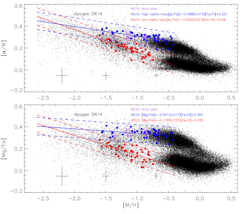
Figure 1: The [M/H] versus $[\alpha/M]$ (upper) and the [M/H] versus [Mg/Fe] (lower) diagrams for our sample stars (black dots). Low-$\alpha$ halo, high-$\alpha$ halo, and thick disk stars from Nissen & Schuster (2010) are shown in red dots, blue dots, and purple pluses, respectively. Linear regressions to these data are shown by red and blue solid lines, and they are shifted by 0.08 dex (dash lines) to selet different groups of stars. Typical errors at $\mbox{\rm[M/H]}\sim-0.7,-1.5$, and $-2.2$ are indicated at the bottom.

3 Halo stars with $|Z|>5$ kpc and the [Mg/Fe] gradient

In the literature, various methods, e.g. selecting nonrotating stars or high velocity stars, can be adopted to pick out halo stars. But the calculation of space velocity requires distance, radial velocity, and proper motions, which are not available for distant stars. With the need of stellar distance and stellar position, the calculation of $|Z|$ is somewhat easier and thus it provides the simplest way to pick out halo stars. That is, we can select stars locating at high $|Z|$, beyond the reach of the disk. Since the scale height of the thick disk is in the range of $0.5-1.0$ kpc (Bland-Hawthorn & Gerhard, 2016), the main population at $|Z|=1-3$ kpc is the thick disk. In view of this, it has been suggested that stars at $|Z|>4$ kpc belong to the halo according to Xue et al. (2008). In this work, we adopt a more strict one, i.e. stars with $|Z|>5$ kpc being the halo sample.

The halo sample is divided into five groups in a $|Z|$ interval of 5 kpc within 20 kpc and of 10 kpc or larger beyond 20 kpc (in order to include enough stars for statistics), i.e. $5<|Z|<10$ kpc, $10<|Z|<15$ kpc, $15<|Z|<20$ kpc, $20<|Z|<30$ kpc and $|Z|>30$ kpc. The distributions of stars in the [M/H] versus [Mg/Fe] diagram are shown in Fig. 2 where all stars with $|Z|>0.5$ kpc are shown in small black dots for comparison. It shows that, at $5<|Z|<10$ kpc, there are two (both high-[Mg/Fe] and low-[Mg/Fe]) sequences in the metallicity range of $-1.1<\mbox{\rm[M/H]}<-0.3$, while the high-[Mg/Fe] sequence with $\mbox{\rm[M/H]}>-1.1$ nearly disappears at $|Z|>10$ kpc. Fig. 3 shows that the relative star number between the high-[Mg/Fe] sequence within $-1.1<\mbox{\rm[M/H]}<-0.6$ and the low-[Mg/Fe] sequence within $-1.6<\mbox{\rm[M/H]}<-1.1$ decreases with $|Z|$ and is close to zero at $|Z|\sim 8$ kpc. In view of this, we further pick out stars at $8<|Z|<10$ kpc, shown as purple dots in the upper left panel of Fig. 2. It is found that most of them belong to the low-[Mg/Fe] sequence clumping at $\mbox{\rm[M/H]}\sim-1.4$, as already noticed by Helmi et al. (2018), with a low fraction of high-[Mg/Fe] stars belonging to the thick disk and/or the in situ halo. Finally, we pick out the most distant stars with $|Z|>30$ kpc, marked by blue dots in the lower right panel. Interestingly, they are found to have systematically lower [Mg/Fe] than those at $20<|Z|<30$ kpc at a given metallicity.

Inspired by this, we suspect that there might be a vertical gradient in the [Mg/Fe] ratio for the halo at $|Z|>10$ kpc. Fig. 4 shows the $|Z|$ and $R$ versus [Mg/Fe] diagrams for all stars at $10<|Z|<60$ kpc and for three separate metallicity ranges, $-1.1<\mbox{\rm[M/H]}<-0.7$, $-1.6<\mbox{\rm[M/H]}<-1.1$, and $-2.6<\mbox{\rm[M/H]}<-1.6$. The reasons for the metallicity divisions at $-0.7$ and $-1.1$ will be given in the next section; they correspond to the transitions between the halo and the disk for the low-[Mg/Fe] and high-[Mg/Fe] sequences. Meanwhile, as described in Sect. 2, the two sequences start to mix together at $\mbox{\rm[M/H]}\sim-1.6$ and thus this is chosen as the start of the metal-poor population in the present work. In Fig. 4, the average [Mg/Fe] at given $|Z|$ and $R$ intervals are indicated by open red squares and single linear fits to them for the whole $|Z|$ or $R$ ranges are shown by blue dash lines. However, the single linear regression is not a good solution for all stars at $|Z|>10$ kpc and for stars in the metallicity range of $-1.1<\mbox{\rm[M/H]}<-0.7$. Moreover, it seems that there is a flat trend of [Mg/Fe] versus $|Z|$ and $R$ at distances larger than 30 kpc for all the three metallicity ranges. Although single linear regression might give a reasonable fit to the data for the metallicity ranges of $-1.6<\mbox{\rm[M/H]}<-1.1$ and $-2.6<\mbox{\rm[M/H]}<-1.6$, we note that a significant number of stars at $|Z|<30$ kpc have $\mbox{\rm[Mg/Fe]}\sim 0.0$ and they deviate significantly from the single linear regression. Instead, they seem to follow the flat trends of stars at distances larger than 30 kpc as an extension into smaller distances of 10-30 kpc.

In view of this, we perform a segment test to the data based on the $fit.seg$ method in R-software by taking into account the errors. We find a break at $|Z|=31$ kpc for all stars and stars with $-1.1<\mbox{\rm[M/H]}<-0.7$, i.e. at $|Z|\sim 30$ kpc in view of the large error at this distance. Then the data are divided into two segments, $|Z|=10-30$ kpc and $|Z|=30-60$ kpc, and two linear regressions are fitted separately. For stars with $-2.6<\mbox{\rm[M/H]}<-1.6$, the regressions are performed for $|Z|<30$ kpc, beyond which only a few stars are present and/or the coverage of $|Z|$ is too narrow to fit. Clearly, in the metallicity range of $-1.1<\mbox{\rm[M/H]}<-0.7$, there are two-segment [Mg/Fe] gradients with different slopes, i.e. $\mbox{\rm[Mg/Fe]}=-0.0071(\pm 0.0010)|Z|+0.181(\pm 0.020)$ ($10<|Z|<30$ kpc) and $\mbox{\rm[Mg/Fe]}=+0.0051(\pm 0.0034)|Z|-0.281(\pm 0.137)$ ($30<|Z|<60$ kpc), with the coefficients of Pearson correlation of $-0.96$ and $+0.73$ and scatters of 0.011 and 0.032 dex, respectively. When the single linear fit to the whole range is adopted, the [Mg/Fe] gradient is of $\mbox{\rm[Mg/Fe]}=-0.0049(\pm 0.0013)|Z|+0.131(\pm 0.039)$ ($10<|Z|<60$ kpc) with a reduced Pearson coefficient of $-0.79$ and a larger scatter of 0.046 dex. It seems that two-segment [Mg/Fe] gradients are preferred for the metallicity range of $-1.1<\mbox{\rm[M/H]}<-0.7$. The two-segment [Mg/Fe] gradient is not prominent for the two metallicity ranges of $-1.6<\mbox{\rm[M/H]}<-1.1$ and $-2.6<\mbox{\rm[M/H]}<-1.6$, partly due to the large uncertainty in abundance at the metal poor end. Further investigation with high precision spectroscopic data for more stars at the outer Galaxy is needed to clarify this topic.

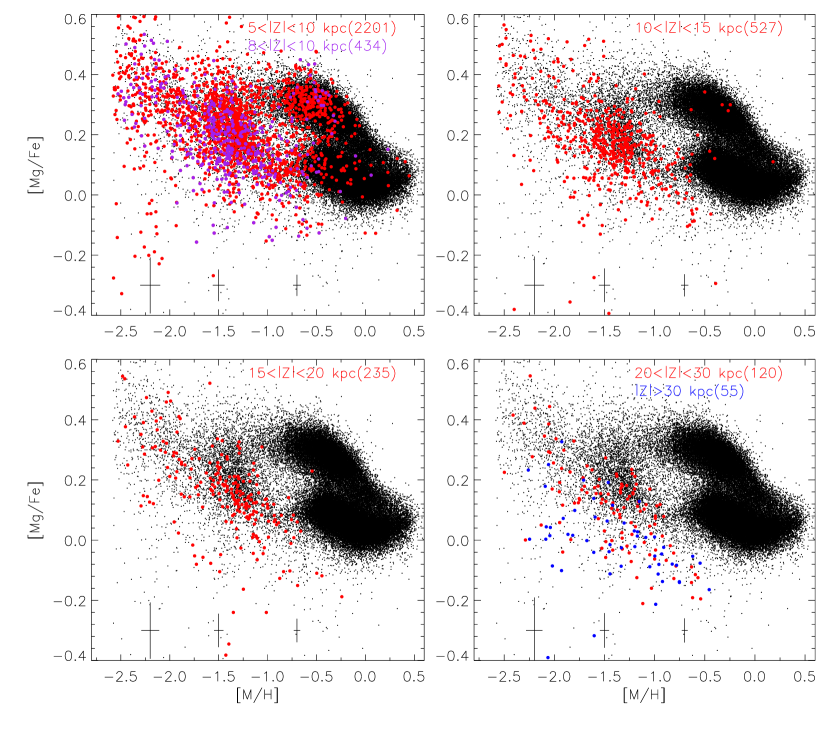
Figure 2: The [M/H] versus [Mg/Fe] distributions for halo stars at $5<|Z|<10$ kpc (including $8<|Z|<10$ kpc), $10<|Z|<15$ kpc, $15<|Z|<20$ kpc, $20<|Z|<30$ kpc and $|Z|>30$ kpc. The star number at each $|Z|$ interval is given in brackets. All stars with $|Z|>0.5$ kpc in our sample are shown by small balck dots for comparison.

Figure 3: Relative star number between the thick disk (TD, $-1.1<\mbox{\rm[M/H]}<-0.6$) and the in situ halo (IH, $-1.6<\mbox{\rm[M/H]}<-1.1$) as a function of $|Z|$ in the high-[Mg/Fe] sequence.

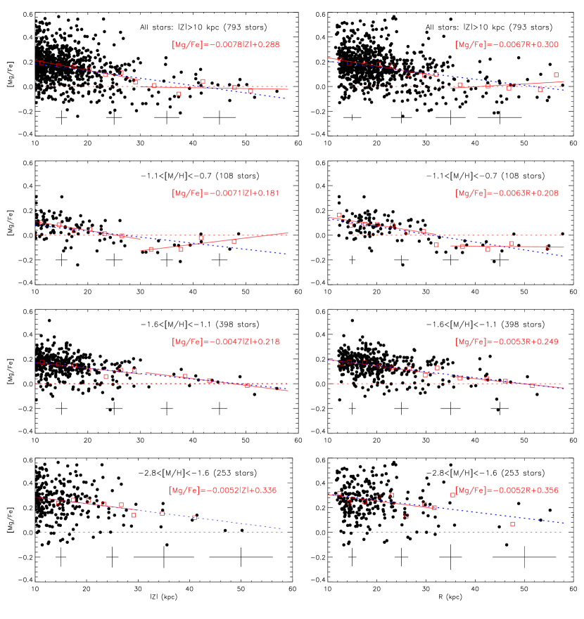
Figure 4: The [Mg/Fe] versus $|Z|$ (left) and $R$ (right) diagrams for all stars at $|Z|>10$ kpc (top) and stars with three metallicity ranges ($-1.1<\mbox{\rm[M/H]}<-0.7$, $-1.6<\mbox{\rm[M/H]}<-1.1$ and $-2.6<\mbox{\rm[M/H]}<-1.6$). Open squares indicate the average [Mg/Fe] ratio at a given $|Z|$ for each bin. Blue dashed lines indicate single linear regressions to open squares for the whole range and red solid lines for the two separate ranges divided at 30 kpc. The star number is given in brackets and the separate regression for the first segment (10-30 kpc) is presented in each panel.

4 Different properties between high-[Mg/Fe] and low-[Mg/Fe] sequences

4.1 The $l$ versus $V_{\rm los}$ diagram

Although stars at $|Z|>5$ kpc mainly belong to the halo population, there are more halo stars located at $|Z|<5$ kpc. Therefore, it is important to select halo stars in a more specific way. Following Hayes et al. (2018), the $l$ versus $V_{\rm los}$ diagram can be adopted to classify disk stars, for which $V_{\rm los}$ shows a sinusoidal variation with Galactic longitude $l$, but there is no such trend for halo stars. Note that the high-[Mg/Fe] sequence includes the thick disk and the in situ halo, and the low-[Mg/Fe] sequence consists of the thin disk and the accreted halo. That is, both sequences have disk and halo stars. Thus, we investigate the $l$ versus $V_{\rm los}$ and $\sigma(\mbox{\rm$V_{\rm los}$})$ diagrams for high-[Mg/Fe] and low-[Mg/Fe] sequences separately in Figures 5 and 6.

Stars within the two dashed red lines in Fig. 1 are selected and the $l$ versus $V_{\rm los}$ diagrams are plotted based on two bin sets: the odd and the even bin sets. For the high-[Mg/Fe] sequence, the odd bin set has [M/H] from $-0.4\pm 0.1$ to $-1.4\pm 0.1$ and the even bin set from $-0.5\pm 0.1$ to $-1.3\pm 0.1$ in steps of 0.2 dex. It is found that the sinusoidal trend in the $l$ versus $V_{\rm los}$ diagram starts to disappear at $-1.3<\mbox{\rm[M/H]}<-1.1$, and there is a hint of such a trend at $-1.2<\mbox{\rm[M/H]}<-1.0$. Thus we define the transition metallicity of $\mbox{\rm[M/H]}\sim-1.1\pm 0.05$ to separate the thick disk and the in situ halo for the high-[Mg/Fe] sequence. In a similar way, the odd bin is set to vary [M/H] from $-0.4\pm 0.1$ to $-1.2\pm 0.1$ and the even bin set from $-0.3\pm 0.1$ to $-1.1\pm 0.1$ in steps of 0.2 dex for the low-[Mg/Fe] sequence. The transition metallicity is defined to be $\mbox{\rm[M/H]}\sim-0.7\pm 0.05$ because the sinusoidal trend disappears at $-0.7<\mbox{\rm[M/H]}<-0.9$, while there is still a sign of such a trend at $-0.8<\mbox{\rm[M/H]}<-0.6$.

Furthermore, the amplitude of the sinusoidal function in each bin also varys with metallicity for both high-[Mg/Fe] and low-[Mg/Fe] sequences, which is consistent with the fact that the disk is kinematically hot and the halo kinematically cold. Quantitatively, the amplitude in the sinusoidal function, calculated to be the mean $V_{\rm los}$ for stars at the $l\sim 85\,deg$ bin, decreases from $82$ to $45\,\mbox{\rm\,$km/s$\,}$ between the two adjacent metallicity bins around $\mbox{\rm[M/H]}\sim-1.1$ in the high-[Mg/Fe] sequence, and a big drop from $120.6$ to $28.5\,\mbox{\rm\,$km/s$\,}$ between the two adjacent metallicity bins at $\mbox{\rm[M/H]}\sim-0.7$ is found in the low-[Mg/Fe] sequence. Meanwhile, the dispersion around the mean $V_{\rm los}$ as a function of $l$ vary significantly with metallicity. As shown in Fig. 6, they start to become large at the transition metallicity ranges of $-1.3<\mbox{\rm[M/H]}<-1.1$ for the high-[Mg/Fe] sequence and of $-0.9<\mbox{\rm[M/H]}<-0.7$ for the low-[Mg/Fe] sequence, generally following in line with the two metallicity divisions via the $l$ versus $V_{\rm los}$ diagram. These variations in amplitude and dispersion of $V_{\rm los}$ provide further support for the separation between the disk and the halo by using this method. In this analysis, we include stars with $|Z|>5$ kpc although this technique usually works for stars not too far from the Galactic plane. And we have checked that the transition metallicities are exactly the same if we limit our sample of stars at $0.5<|Z|<5$ kpc only. Finally, we notice that the two metallicity divisions are consistent with the results in the literature. For the low-$\alpha$ sequence, Hawkins et al. (2015) suggested that the low metallicity end of the thin disk is at $\mbox{\rm[M/H]}\sim-0.7$, below which it belongs to the accreted halo, and the metallicity division at $\mbox{\rm[M/H]}\sim-1.1$ for the high-[Mg/Fe] sequence is exactly the same as that of Fernandez-Alvar et al. (2018).

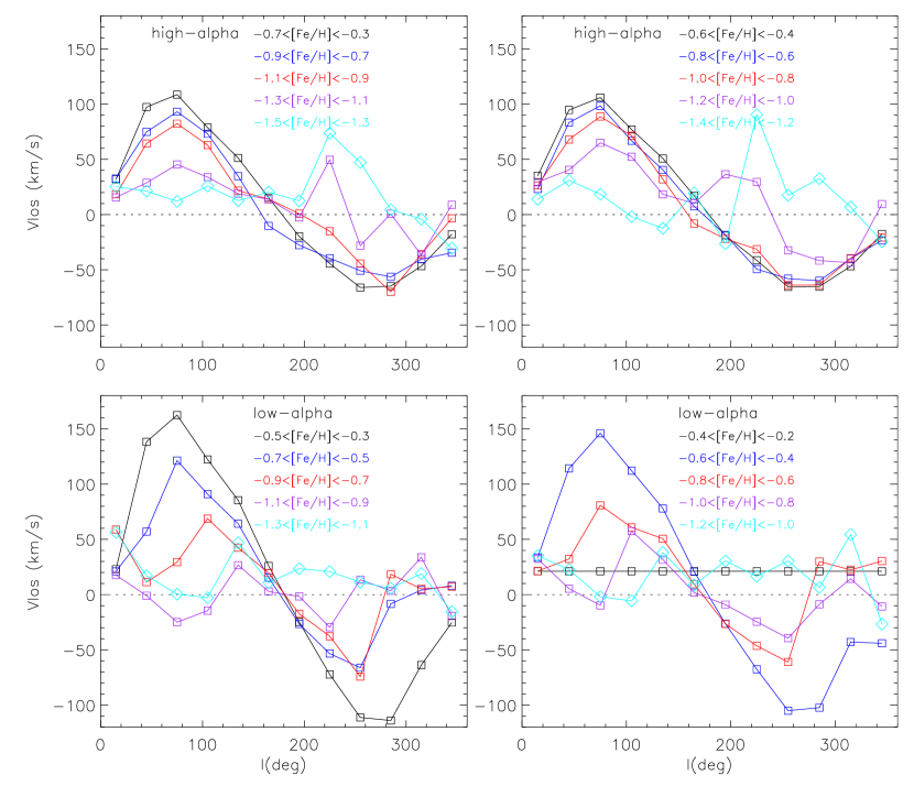
Figure 5: The $l$ versus $V_{\rm los}$ diagrams for the high-[Mg/Fe] (upper) and low-[Mg/Fe] (bottom) sequences with different colors indicating stars in different metallicity intervals.

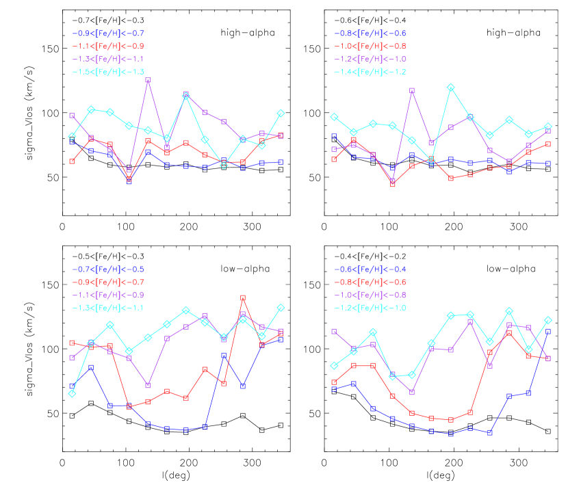
Figure 6: The $l$ versus $\sigma(\mbox{\rm$V_{\rm los}$})$ diagrams for the high-[Mg/Fe] (upper) and low-[Mg/Fe] (bottom) sequences. The symbols and colors are the same as those in Figure 5.

4.2 The $R$ and $|Z|$ distributions

After setting the metallicity boundaries between the halo and the disk for the two [Mg/Fe] sequences in the [M/H] versus [Mg/Fe] diagram, we divide our sample into four groups of stars, i.e. the high-[Mg/Fe] thick disk with $-1.1<\mbox{\rm[M/H]}<-0.7$ (cyan dots), the high-[Mg/Fe] in situ halo with $-1.6<\mbox{\rm[M/H]}<-1.1$ (blue crosses), and the low-[Mg/Fe] accreted halo at the same two metallicity ranges (red and purple dots). Then we compare the relative distributions of star number among the four groups of stars as functions of $R$ (Galactocentric distance) and $|Z|$ (vertical distance to the plane) in the left panel of Fig. 7. It shows that they all peak at $R\sim 8-10$ kpc and $|Z|<5$ kpc, which indicates that the halo and the disk mix significantly in the inner Galaxy. However, there is a big difference in relative fraction of star number between high-[Mg/Fe] and low-[Mg/Fe] sequence at larger distances. In particular, the high-[Mg/Fe] thick disk (cyan line) and the in situ halo (blue line) show a cutoff at $R\sim 15$ kpc and $|Z|\sim 10$ kpc, beyond which the low-[Mg/Fe] accreted halo (red and purple lines) still contributes substantially, as is clearly shown in the corresponding subfigures of Fig. 7.

In the right panel of Fig. 7, the low-[Mg/Fe] accreted halo at the same two metallicity ranges (red and purple dots) are compared with more metal-poor halo with $-2.0<\mbox{\rm[M/H]}<-1.6$ (orange) and $-2.6<\mbox{\rm[M/H]}<-2.0$ (aqua). Similarly, the two groups of stars from the low-[Mg/Fe] accreted halo peak at $R\sim 8-10$ kpc and $|Z|<5$ kpc as the reference samples, but they persist to overpopulate at larger distances of $R>15$ kpc and $|Z|>10$ kpc. Although the overpopulation of low-[Mg/Fe] accreted halo at $-1.1<\mbox{\rm[M/H]}<-0.7$ and $-1.6<\mbox{\rm[M/H]}<-1.1$ is weaker than the comparison with stars in the high-[Mg/Fe] sequence, red and/or purple lines outnumber the orange/aqua lines by $3-5$ times, as seen in the subfigures of the right panel of Fig. 7.

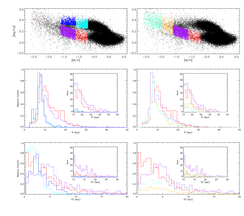
Figure 7: Comparison of the low-[Mg/Fe] accreted halo at $-1.1<\mbox{\rm[M/H]}<-0.7$ (red dots and lines) and $-1.6<\mbox{\rm[M/H]}<-1.1$ (purple dots and lines) with two sets of reference groups. Left: the high-[Mg/Fe] thick disk with $-1.1<\mbox{\rm[M/H]}<-0.7$ (cyan dots and lines) and the high-[Mg/Fe] in situ halo with $-1.6<\mbox{\rm[M/H]}<-1.1$ (blue dots and lines). Right: the more metal-poor halo with mixing high-[Mg/Fe] and low-[Mg/Fe] populations at $-2.0<\mbox{\rm[M/H]}<-1.6$ (orange dots and lines) and $-2.6<\mbox{\rm[M/H]}<-2.0$ (aqua dots and lines). In the subfigures, we compare the distributions of star number at larger distances of $R>15$ kpc and $|Z|>10$ kpc.

4.3 The metallicity gradients

It is interesting to compare the metallicity gradient between the high-[Mg/Fe] and low-[Mg/Fe] sequences in order to understand the formation scenarios of the Galactic halo. In the left panel of Fig. 8, we plot the [M/H] versus $|Z|$ for stars with $-1.6<\mbox{\rm[M/H]}<-0.7$, which is the metallicity range where the two [Mg/Fe] sequences are well separated. Interestingly, for stars at $|Z|<8$ kpc, metallicity gradients exist for both high-[Mg/Fe] and low-[Mg/Fe] sequences with coefficients of Pearson correlation of 0.96 in both cases. However, we notice that the former has a steeper slope ($-0.053\pm 0.005$) than the latter ($-0.037\pm 0.006$). At larger $|Z|$, mean metallicity seems to remain flat for the low-[Mg/Fe] sequence. On close inspection of the bottom left panel of Fig. 8, it is found that the main reason for this difference may come from the inclusion of the high-[Mg/Fe] thick disk stars with $-1.1<\mbox{\rm[M/H]}<-0.7$. It may be more reasonable to limit this comparison at a narrow metallicity range of $-1.6<\mbox{\rm[M/H]}<-1.1$. As shown in the right panel of Fig. 8, there is no significant trend for the low-[Mg/Fe] sequence until $|Z|\sim 20$ kpc but there is a hint of a small slope of $-0.015\pm 0.003$ with a coefficient of the Pearson correlation of 0.88 for the high-[Mg/Fe] sequence at $0<|Z|<8$ kpc, beyond which the number of stars is too small for a good statistic. For the more metal poor end at $-2.0<\mbox{\rm[M/H]}<-1.6$ and $-2.6<\mbox{\rm[M/H]}<-2.0$, Fig. 9 shows no slope in the [M/H] versus $|Z|$ diagram for the whole $0<|Z|<20$ kpc range, but there is a hint of a possible gradient for $0<|Z|<8$ kpc. In this comparison, we use $|Z|$, rather than $R$, in order to reduce the contribution from the Galactic disk. We note that the Galactic disk is mainly limited within $|Z|<5$ kpc, while the Galactocentric distances ($R$) of disk stars beyond solar circle (at 8 kpc) could reach farther than 15 kpc (Bland-Hawthorn & Gerhard, 2016). Thus, the metallicity gradient of the Galactic halo, if existed, would be clearer in the vertical $|Z|$ direction than the Galactocentric distances $R$.

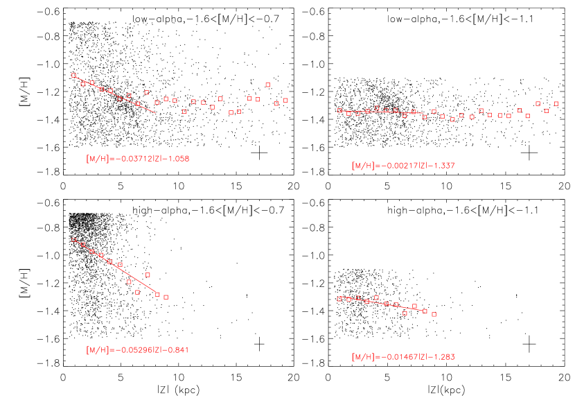
Figure 8: Metallicity gradients for low-[Mg/Fe] and high-[Mg/Fe] sequences in the two metallicity ranges of $-1.6<\mbox{\rm[M/H]}<-0.7$ and $-1.6<\mbox{\rm[M/H]}<-1.1$. Open squares are the mean metallicities at given $|Z|$ and solid lines are linear regressions to the data at $|Z|<8$ kpc.

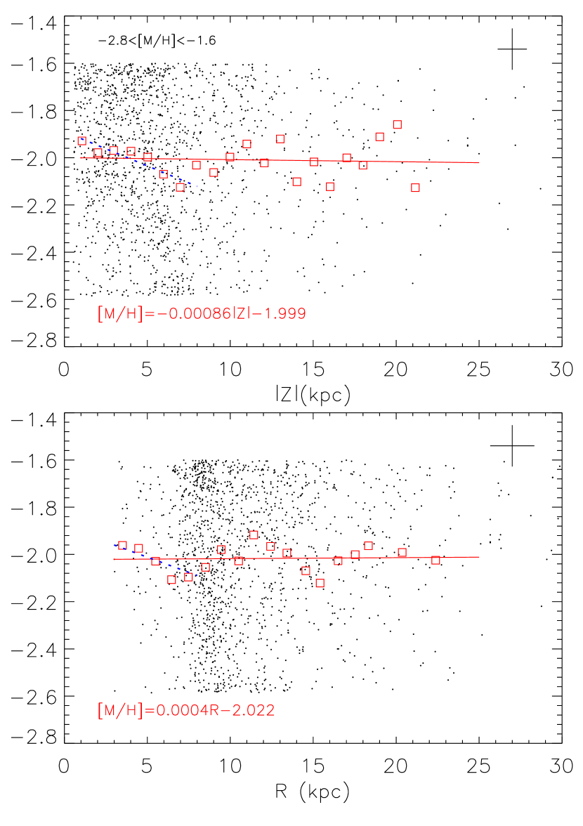
Figure 9: The metallicity gradients for metal poor stars at $-2.0<\mbox{\rm[M/H]}<-1.6$ and $-2.6<\mbox{\rm[M/H]}<-2.0$. The symbols are the same as Fig. 8.

5 Implications and Conclusions

Based on the APOGEE DR14 and the distance catalog, we investigate the space distributions, $V_{\rm los}$ variations along Galactic longitude, and abundance gradients between the high-[Mg/Fe] and low-[Mg/Fe] sequences in the [M/H] versus [Mg/Fe] diagram. In particular, we investigate the distributions of the two [$\alpha$/Fe] sequences far beyond the solar vicinity ($D<5$ kpc) for the first time.

The main results of the present work are summarized as follows. The two [Mg/Fe] sequences are clearly shown for stars at $5<|Z|<10$ kpc and well separated in the intermediate-metallicity range of $-1.1<\mbox{\rm[M/H]}<-0.7$. In the [M/H] versus [Mg/Fe] diagram, the transition metallicity of the halo from the disk is found at $\mbox{\rm[M/H]}\sim-0.7\pm 0.05$ for the low-[Mg/Fe] sequence and of $\mbox{\rm[M/H]}\sim-1.1\pm 0.05$ for the high-[Mg/Fe] sequence by investigating the $l$ versus $V_{\rm los}$ diagrams with different metallicity bins. Both the high-[Mg/Fe] thick disk with $\mbox{\rm[M/H]}>-1.1$ and the in situ halo with $-1.6<\mbox{\rm[M/H]}<-1.1$ have a cutoff at $R\sim 15$ kpc and $|Z|\sim 8-10$ kpc, beyond which the low-[Mg/Fe] accreted halo with $-1.6<\mbox{\rm[M/H]}<-0.7$ is dominating. There is a negative [Mg/Fe] gradient for stars at $|Z|>10$ kpc in the metallicity range of $-1.1<\mbox{\rm[M/H]}<-0.7$, but it flattens out at $|Z|\sim 30$ kpc. In the metallicity range of $-2.6<\mbox{\rm[M/H]}<-1.1$, most stars follow a negative [Mg/Fe] gradient at $|Z|=10-30$ kpc, but a constant $\mbox{\rm[Mg/Fe]}\sim 0.0$ is found for a small fraction of stars at $|Z|=10-30$ kpc and it extends outward at $|Z|>30$ kpc. In the intermediate-metallicity range of $-1.6<\mbox{\rm[M/H]}<-1.1$, the $\mbox{\rm[M/H]}-|Z|$ gradient exists at $|Z|<8$ kpc for the high-[Mg/Fe] sequence, while there is no such trend for the low-[Mg/Fe] sequence.

Based on these results, we may suggest a three-section halo with different chemical properties: the inner in situ halo at $|Z|<8-10$ kpc with high-[Mg/Fe] and a metallicity gradient, the intermediately outer halo at $10<|Z|<30$ kpc without metallicity gradient but with dual-mode [Mg/Fe] gradient, and the extremely outer accreted halo with $|Z|>30$ kpc without both metallicity and [Mg/Fe] gradients. This suggestion is consistent with the transition of the dual-mode halo at $R\sim 15-20$ kpc and the radius break at $R\sim 30-45$ kpc in the spatial density distribution of halo stars as already described in the Introduction of the present work. We emphasize that the selection effect of the APOGEE survey is not considered in the present paper. But we note that Nandakumar et al. (2017) found a negligible selection function effect on the metallicity distribution function and the vertical metallicity gradients for the APOGEE survey. In view of this, we expect that our derived [Mg/Fe] and metallicity gradients may not be affected by the selection effect. Further investigations on more precise observations and theoretical simulations are desirable to discover the formation of the Galaxy. In particular, the star number at the distant region of the Galaxy is too small presently and we need a deeper spectroscopic survey in the future. Meanwhile, the improvement on the distance scale for distant stars is desirable to ensure that they have precision as good as that of nearby stars. Future Thirty Meter Telescope equipped with high-resolution spectrographs in both near infrared and optical bands is awaiting an opportunity to explore a high-precision chemical map of the extremely outer halo of the Galaxy.

References

- Abadi et al. (2006) Abadi, M.G., Navarro, J.F., Steinmetz, M., 2006, MN, 365, 747
- Abolfathi et al. (2018) Abolfathi, B., Aguado, D. S., Aguilar, G., et al. 2018, ApJS, 235, 42
- Akhter et al. (2012) Akhter, S., Da Costa, G.S., Keller, S.C., Schmidt, B.P.,2012,ApJ,756,23
- Babusiaux et al. (2018) Gaia Collaboration,Babusiaux, C., van Leeuwen, F.,; Barstow, M. A., et al. 2018, A&A, 616, A10.
- Bland-Hawthorn & Gerhard (2016) Bland-Hawthorn, J., & Gerhard O., 2016, ARA&A, 54, 529
- Blanton et al. (2017) Blanton, M.R., Bershady, M.A., Abolfathi, B. et al. 2017, AJ, 154, 28
- Bressan et al. (2012) Bressan, A., Marigo, P., Girardi, L. et al. 2012, MNRAS, 427, 127
- Bullock & Johnston (2005) Bullock, J. S., & Johnston, K. V. 2005, ApJ, 635, 931
- Carollo et al. (2010) Carollo, D., Beers, T. C., Chiba, M., et al. 2010, ApJ, 712, 692
- Chen et al. (2014) Chen, Y. Q., Zhao, G., Carrell, K., et al. 2014, ApJ, 795, 52
- Dinescu, Girard & van Altena (1999) Dinescu, D.I., Girard, T.M. & van Altena, W.F. 1999, AJ, 117, 1792
- Eggen, Lynden-Bell & Sandage (1962) Eggen O. J., Lynden-Bell D., Sandage A. R., 1962, ApJ, 136, 748
- Font et al. (2011) Font, A. S., McCarthy, I. G., Crain, R. A., et al. 2011, MNRAS, 416, 2802
- Fernandez-Alvar et al. (2015) Fernandez-Alvar, E., Allende Prieto, C., Schlesinger, K. J., et al. 2015, A&A, 577, 81
- Fernandez-Alvar et al. (2018) Fernandez-Alvar, E., Tissera, P.B. Carigi, L. et al. 2018, astro-ph/1809.02368
- García et al. (2016) Garcïa Perez, A. E., Allende Prieto, C., Holtzman, J. A., et al. 2016, AJ, 151, 144
- Gunn et al. (2006) Gunn, J. E., Siegmund, W. A., Mannery, E. J., et al. 2006, AJ, 131, 2332
- Hayes et al. (2018) Hayes, C.R., Majewski, S.R., Hasselquist, S. et al. 2018, ApJ, 852, 49
- Haywood et al. (2018) Haywood, M., Di Matteo, P., Lehnert, M., Snaith, O., Khoperskov, S., Gömez, A., 2018, ApJ, 863, 113
- Hawkins et al. (2015) Hawkins, K., Jofre, P., Masseron, T., & Gilmore, G. 2015, MNRAS, 453, 758
- Helmi et al. (2018) Helmi, A., Babusiaux, C., Koppelman, H.H., Massari, D., Veljanoski, J., Brown, G. A., 2018, Nature, 563, 85
- Holtzman et al. (2018) Holtzman, J.A., Hasselquist, S., Shetrone, M., et al. 2018, AJ, 156, 125
- Kellerr et al. (2008) Keller, S.C., Murphy, S., Prior, S. et al. 2008, ApJ, 678, 851
- Majewski et al. (2017) Majewski, S. R., Schiavon, R. P., Frinchaboy, P. M., et al. 2017, AJ, 154, 94
- Myeong et al. (2018) Myeong, G.C., Evans, N.W., Belokurov, V., Sanders, J.L. & Koposov, S.E. 2018, MNRAS, 478, 5449
- McCarthy et al. (2012) McCarthy, I. G., Font, A. S., Crain, R. A., et al. 2012, MNRAS, 420, 2245
- Nandakumar et al. (2017) Nandakumar, G., Schultheis, M., Hayden, M. et al. 2017, A&A, 606, 97
- Nissen & Schuster (2010) Nissen, P.E. & Schuster, J.W. 2010, A&A, 110, 666
- Queiroz et al. (2018) , A. B. A., Anders, F., Santiago, B. X et al., 2018, MNRAS, 476, 2556
- Santiago et al. (2016) Santiago, B.X., Brauer, D.E., Anders, F., 2016, A&A, 585, 42
- Searle & Zinn (1978) Searle L.,& Zinn R., 1978, ApJ, 225, 357
- Tolstoy et al. (2009) Tolstoy, E., Hill, V.,; Tosi, M., 2009, ARA&A, 47, 371
- Wang et al. (2016) Wang, J.L.l, Shi, J.R., Pan, K.K. et al. 2016, MNRAS, 460, 3179
- Wilson et al. (2010) Wilson, J. C., Hearty, F., Skrutskie,M. F., et al. 2010, Proc. SPIE, 7735, 77351
- Xue et al. (2008) Xue, X.X. et al. 2008, ApJ, 684, 1143
- Zolotov et al. (2009) Zolotov A., Willman B., Brooks A. M., Governato F., Brook C. B., Hogg D. W., Quinn T., Stinson G., 2009, ApJ, 702, 1058