Are your Items in Order?

Abstract

Items in many datasets can be arranged to a natural order. Such orders are useful since they can provide new knowledge about the data and may ease further data exploration and visualization. Our goal in this paper is to define a statistically well-founded and an objective score measuring the quality of an order. Such a measure can be used for determining whether the current order has any valuable information or can it be discarded.

Intuitively, we say that the order is good if dependent attributes are close to each other. To define the order score we fit an order-sensitive model to the dataset. Our model resembles a Markov chain model, that is, the attributes depend only on the immediate neighbors. The score of the order is the BIC score of the best model. For computing the measure we introduce a fast dynamic program. The score is then compared against random orders: if it is better than the scores of the random orders, we say that the order is good. We also show the asymptotic connection between the score function and the number of free parameters of the model. In addition, we introduce a simple greedy approach for finding an order with a good score. We evaluate the score for synthetic and real datasets using different spectral orders and the orders obtained with the greedy method.

1 Introduction

Seriation, discovering a linear order for the attributes, is a popular topic in data mining. The motivation for ordering the attributes comes from the fact that many datasets have an inherent order, for example, the location of genes in gene amplification data. In fields such as paleontology [1] or archaeology [2] discovering the order (age) of the sites is a fundamental question. There are many benefits once the order has been discovered. The data can visualized as a binary matrix for further analysis. Also, the complexity of certain data mining algorithms, for example discovering tiles [3], can be reduced when we restrict ourselves to the discovered order.

In this paper, we study measuring the quality of a given attribute order. Such a measure will help us to determine whether the order at hand is genuinely significant. We propose an intuitive and novel method for measuring the quality. In our approach an order is good if the attributes that are dependent of each other are close in the given order.

Example 1

Assume that we have a dataset with 5 items, $a_{1},\ldots,a_{5}$, in which the value of attribute $a_{i}$ is generated from the value of the previous attribute $a_{i-1}$ by copying it and flipping it with a (small) probability. We may now conclude that here the original order is good. Whereas, for example, an order $a_{1},a_{4},a_{3},a_{5},a_{2}$ is bad since the attributes $a_{1}$ and $a_{2}$ are far away from each other.

Our measure is a generalization of the idea given in the example. Given a dataset and an order we build a model that depends on the order. Our construction will be such that model is simple and has good likelihood if the dependent attributes are close. As a measure for goodness of the model we will use Bayesian Information Criteria (BIC) which favors simple models that fit data well. It turns out that we can find the model with the best BIC score through a fast dynamic program.

Also, our model can be seen as a Markov Random Field (MRF) model in which the the items depend only on their immediate neighbors (see, for example, [4] for introduction to MRF).

We compare the score of the discovered model against the scores of random orders, for example, we consider the probability that a random order will have a better score than the score of the given model. The probability is close to $0$, if the order under investigation has an exceptionally good score.

We study the asymptotic behavior of the score and show that asymptotically it is an increasing function of the number of free model parameters. Such a behavior is natural since we favor simple models yet surprising since the BIC penalty, the term through which the degree of freedom affects the score, vanishes as the number of data points grows.

The rest of the paper is organized as follows. The preliminaries are given in Section 2 and the model itself is defined in Section 3. We explain the dynamic program for finding the best in Section 4. In Section 5 we consider spectral and greedy methods for inducing the order. In Section 6 we compare the score with random orders. We discuss the asymptotic behavior in Section 7. Section 9 is devoted to the related work and in Section 8 we describe our empirical results. Finally, we conclude the paper with a discussion in Section 10.

2 Preliminaries and Notation

In this section we introduce the preliminaries and notation that we will use in subsequent sections.

A transaction $t\in\left\{0,1\right\}^{K}$ is a binary vector of length $K$. A binary dataset is a collection of $N$ transactions having the length $K$. We can easily visualize the dataset as a binary matrix of size $N\times K$. We use the notation of ${\left|D\right|}=N$ to express the number of transactions in $D$. An attribute $a_{i}$, $i=1,\ldots,K$, is a random Bernoulli variable representing the $i$th element in a random transaction. We set $A=\left\{a_{1},\ldots,a_{K}\right\}$ to be the collection of all attributes.

Assume that we are given a distribution $p$ defined over a space of binary vectors $\left\{0,1\right\}^{K}$. Let $X=\left\{x_{1},\ldots,x_{L}\right\}\subseteq A$ be the collection of attributes. Let $v=\left\{0,1\right\}^{L}$ be a binary vector of length $L$. We use the notation $p\mathopen{}\left(X=v\right)$ to mean the probability $p\left(x_{1}=v_{1},\ldots,x_{L}=v_{L}\right)$.

Given a binary dataset $D$ we define $q_{D}$, an empirical distribution to be

$$q_{D}\mathopen{}\left(A=v\right)=\frac{{\left|\left\{t\in D;t=v\right\}\right|}}{{\left|D\right|}}.$$

We assume that there is a specific linear order induced on the attributes. Such an order can be identified with a permutation function $o$ mapping from $\left(1,\ldots,K\right)$ to $\left(1,\ldots,K\right)$. To ease the notation we often assume that $o$ is the identity permutation, that is $o(i)=i$. Let $X$ be a collection of attributes, we say that $X$ is an item segment if $X$ contains only consecutive attributes. For example, $a_{o(1)}a_{o(2)}a_{o(3)}$ is an item segment, however, $a_{o(1)}a_{o(2)}a_{o(4)}$ is not since $a_{o(3)}$ is missing.

The entropy of an item segment $X$ w.r.t. to the distribution $p$, denoted by $H\mathopen{}\left(X;p\right)$, is

$$H\mathopen{}\left(X;p\right)=-\sum_{v}p\mathopen{}\left(X=v\right)\log p\mathopen{}\left(X=v\right),$$

where the usual convention $0\times\log 0=0$ is used. All the logarithms in this paper is of base $2$. We will shorten $H\mathopen{}\left(A;p\right)$ into $H\mathopen{}\left(p\right)$. We also write $H\mathopen{}\left(X;D\right)$ to mean $H\mathopen{}\left(X;q_{D}\right)$.

3 Order-sensitive Model

In this section we define our model that is based on the order of the attributes. Informally, our approach is based on generalizing simple markov chain model demonstrated in Example 1. We generalize this by allowing the item $a_{i}$ to depend on several previous items. However, we require that if $a_{i}$ depends on $a_{j}$, then it also must depend on all items between $a_{j}$ and $a_{i}$. Thus, our model will be simple if the dependent items are close to each other.

In order to make the preceeding discussion more formal, assume that we are given a cover of item segments $\mathcal{C}=\left\{C_{1},\ldots,C_{L}\right\}$, that is, $\bigcup_{i}C_{i}=A$. We assume that there is no $C_{i},C_{j}\in\mathcal{C}$ such that $C_{i}\subset C_{j}$, that is, $\mathcal{C}$ is an antichain. We also assume that $\mathcal{C}$ is ordered based on the first attribute of each segment $C_{i}$. We define $\mathrm{seg}\mathopen{}\left(o\right)$ to be the family of all such collections. Given the collection $\mathcal{C}$ we define a model $M\mathopen{}\left(\mathcal{C}\right)$ to be a collection of distributions that can be expressed as

(3.1) $$p\mathopen{}\left(A\right)=\frac{\prod_{i=1}^{L}p\mathopen{}\left(C_{i}\right)}{\prod_{i=1}^{L-1}p\mathopen{}\left(S_{i}\right)}=p\mathopen{}\left(C_{1}\right)\prod_{i=1}^{L-1}p\mathopen{}\left(C_{i+1}-C_{i}\mid S_{i}\right),$$

where $S_{i}=C_{i+1}\cap C_{i}$. That is, the attributes in $C_{i}-C_{i-1}$ depend only on their immediate neighbors, $C_{i}\cap C_{i-1}$.

Example 2

Assume that $\mathcal{C}=\left\{\left\{a_{1}\right\},\ldots,\left\{a_{K}\right\}\right\}$, that is, each segment is simply a singleton. Then the attributes according to any distribution $p\in M\mathopen{}\left(\mathcal{C}\right)$ are independent, $p\mathopen{}\left(A\right)=\prod_{i}^{K}p\mathopen{}\left(a_{i}\right)$.

The distribution $p$ used to generate data in Example 1 can be written as

$$p(a_{1})p(a_{2}\mid a_{1})\cdots p(a_{5}\mid a_{4})=\frac{\prod_{i=1}^{4}p(a_{i}a_{i+1})}{\prod_{i=2}^{4}p(a_{i})}.$$

Hence, $p\in M\mathopen{}\left(\left\{a_{1}a_{2},a_{2}a_{3},a_{3}a_{4},a_{4}a_{5}\right\}\right)$.

The other extreme is that $\mathcal{C}$ contains only one segment containing all items, $\mathcal{C}=\left\{A\right\}$. In this case the distribution maximizing the likelihood is the empirical distribution, $q_{D}\mathopen{}\left(A\right)$. More generally, if $\mathcal{C}$ is an ordered partition of $A$, that is, $C_{i}\cap C_{i-1}=\emptyset$, then the distribution $p\in M\mathopen{}\left(\mathcal{C}\right)$ has independent components $C_{i}$, $p\mathopen{}\left(A\right)=\prod p\mathopen{}\left(C_{i}\right)$. Hence we can view the general model as a generalization of a partition of $A$ by allowing the segments to overlap.

Given a dataset $D$ we define $p^{*}$ to be the the unique distribution from $M\mathopen{}\left(\mathcal{C}\right)$ such that $p^{*}\mathopen{}\left(C_{i}=t\right)=q_{D}\mathopen{}\left(C_{i}=t\right)$ for any $C_{i}\in\mathcal{C}$ and any binary vector $t$ of length ${\left|C_{i}\right|}$. We wish to show that $p^{*}$ maximizes the log-likelihood of $D$. To see this, let $p\in M\mathopen{}\left(\mathcal{C}\right)$. Let us write $S_{i}=C_{i}\cap C_{i+1}$. Then we have

$$\begin{split}&\log p^{*}(D)-\log p(D)\\ &\quad={\left|D\right|}\sum_{i=1}^{L}\sum_{t}p^{*}(A=t)\log\frac{p^{*}(C_{i}=t_{C_{i}})}{p(C_{i}=t_{C_{i}})}.\\ \end{split}$$

The last equation is the (scaled) Kullback-Leibler divergence between $p^{*}$ and $p$ It is always non-negative and is $0$ if and only if $p=p^{*}$. Hence $p^{*}$ maximizes the likelihood.

Let us compute the the log-likelihood of $D$ given a distribution $p^{*}\in M\mathopen{}\left(\mathcal{C}\right)$, that is, the distribution maximizing the likelihood. Let $S_{i}=C_{i}\cap C_{i+1}$. A straightforward calculation reveals that the log-likelihood can be rewritten as a sum of entropies,

(3.2) $$\begin{split}\log p^{*}\mathopen{}\left(D\right)&=\sum_{t\in D}\log p^{*}\mathopen{}\left(A=t\right)\\ &=-{\left|D\right|}\sum_{i=1}^{L}H\mathopen{}\left(C_{i};D\right)+{\left|D\right|}\sum_{i=1}^{L-1}H\mathopen{}\left(S_{i};D\right).\end{split}$$

Our goal is to find a collection $\mathcal{C}$ for which the model provides high likelihood. The problem is that the model with the highest likelihood would be always for the collection $\mathcal{C}=\left\{A\right\}$, for which the optimal distribution is simply the empirical distribution. To keep it from this behaviour we will use Bayesian Information Criteria (BIC) to punish more complex models over the simple ones [5]. Hence, our goal is to minimize the BIC cost function,

$$-\log p^{*}(D)+\frac{\log{\left|D\right|}}{2}\mathrm{deg}\mathopen{}\left(\mathcal{C}\right),$$

where $\mathrm{deg}\mathopen{}\left(\mathcal{C}\right)$ is the number of free parameters in the model $M\mathopen{}\left(\mathcal{C}\right)$. To compute the number of free parameters, let us consider the right side of Eq. 3.1. The first component $p(C_{1})$ can be parameterized with a real vector of length $2^{{\left|C_{1}\right|}}-1$. Similarly, the $i$th component can be parameterized with a vector of length $2^{{\left|C_{i}\right|}-{\left|S_{i-1}\right|}}-1$. Since the $i$th component depends on the values of $S_{i-1}$ we need parameters for each combination of values of $S_{i-1}$. There are $2^{{\left|S_{i-1}\right|}}$ such values. The total number of free parameters is then equal to

(3.3) $$\begin{split}\mathrm{deg}\mathopen{}\left(\mathcal{C}\right)&=2^{{\left|C_{1}\right|}}-1+\sum_{i=2}^{L}2^{{\left|S_{i-1}\right|}}\left(2^{{\left|C_{i}\right|}-{\left|S_{i-1}\right|}}-1\right)\\ &=\sum_{i=1}^{L}2^{{\left|C_{i}\right|}}-1-\sum_{i=1}^{L-1}2^{{\left|S_{i}\right|}}-1.\end{split}$$

In order to compute the BIC score we can combine Eqs. 3.2–3.3 in the following way. We define a score $s\mathopen{}\left(C\right)$ for an item segment $C$ to be

$$s\mathopen{}\left(C\right)={\left|D\right|}H\mathopen{}\left(C;D\right)+\frac{\log{{\left|D\right|}}}{2}\left(2^{{\left|C\right|}}-1\right).$$

Similarly, given a collection $\mathcal{C}=\left\{C_{1},\ldots,C_{L}\right\}$ of item segments we define

(3.4) $$s\mathopen{}\left(\mathcal{C}\right)=\sum_{i=1}^{L}s\mathopen{}\left(C_{i}\right)-\sum_{i=1}^{L-1}s\mathopen{}\left(S_{i}\right),$$

that is, $s\mathopen{}\left(\mathcal{C}\right)$ is the sum of the negative likelihood of the optimal distribution in $M\mathopen{}\left(\mathcal{C}\right)$ and the BIC penalty term. Given an order $o$ we define $s\mathopen{}\left(o\right)$ to be the score of the best possible model,

$$s\mathopen{}\left(o\right)=\min\left(s\mathopen{}\left(\mathcal{C}\right)\mid\mathcal{C}\in\mathrm{seg}\mathopen{}\left(o\right)\right).$$

It is easy to see that minimizing the score produces simple models having high likelihood of the data. Note that if the dependent attributes are close to each other, the segments will be short. Hence the BIC punishment will be small. However, if the dependent attributes are far away, then the segments must be long and the BIC penalty is far greater. Hence, our score favors orders in which dependent attributes are close to each other.

Example 3

Assume that we have a dataset $D$ given by

(3.5) $$D=\left[\begin{array}[]{ccccc}1&1&1&0&0\\ 1&0&1&0&0\\ 0&0&0&1&1\\ 1&0&1&1&1\\ 0&0&0&0&1\\ \end{array}\right].$$

Assume also that our model is $\mathcal{C}=\left\{ab,\,bcd,\,de\right\}$. We have $S_{1}=C_{1}\cap C_{2}=b$ and $S_{2}=C_{2}\cap C_{3}=d$. The entropies for the segments are

$$\begin{split}H\mathopen{}\left(C_{1}\right)=1.52,&\ H\mathopen{}\left(C_{2}\right)=2.32,H\mathopen{}\left(C_{3}\right)=1.52,\\ H\mathopen{}\left(S_{1}\right)=0.72,&\text{ and }H\mathopen{}\left(S_{2}\right)=0.97.\end{split}$$

Hence the final score is

$$\begin{split}s\mathopen{}\left(\mathcal{C}\right)=&5\times\left(1.52+2.32+1.52-0.72-0.97\right)\\ &+\frac{\log 5}{2}\left(3+7+3-1-1\right)=31.13.\end{split}$$

We will finish this section by discussing the connection between the order and Bayesian networks. Our model can be seen as a Bayesian network, where item $a_{i}$ is a parent of $a_{j}$, if and only if $i<j$ and $a_{i}$ and $a_{j}$ belongs to the same segment (see Figure 1 for an example).

Figure 1: A toy example of an order-sensitive model. The model can be viewed as a special type of Bayes Network.

If we interpret our model as a Bayesian network, then it is easy to see that $p^{*}(a_{i}\mid\mathit{par}\mathopen{}\left(a_{i}\right))=q_{D}(a_{i}\mid\mathit{par}\mathopen{}\left(a_{i}\right))$. In other words, the distribution $p^{*}$ is the maximum-likelihood estimate of the corresponding Bayesian network. In fact, the factorization of the BIC score in Eq. 3.4 is equivalent to the factorization obtained by performing a junction tree decomposition (see [4]) to the network. However, interpreting the model as a Bayesian network is somewhat misleading, since our model does not change if we reverse the order of the items.

4 Finding the Optimal Model

In this section we demonstrate how we can find the collection of item segments having the minimal score $s\mathopen{}\left(\mathcal{C}\right)$. We do this by constructing a dynamic program. Furthermore, we demonstrate how we can prune a large amount of long segments, and thus reducing the required execution time. In addition, we discuss how to efficiently compute the entropy using a particular tree structure.

4.1 Forming the Dynamic Program

Our goal is to find a collection $\mathcal{C}$ for which the score $s\mathopen{}\left(\mathcal{C}\right)$ is the smallest possible. We achieve this by using dynamic program and solving subproblems. In order to do this we set $f\mathopen{}\left(i,j\right)$ to be the best collection of segments covering the attributes $\left\{a_{i},\ldots,a_{K}\right\}$ such that the first segment has the attribute $a_{j}$ The optimal collection would be then $f\mathopen{}\left(1,1\right)$.

To compute the values of $f$ we use the following order:

$$\begin{split}f(K,K),f(K-1,K),f(K-1,K-1),\ldots\qquad\\ \qquad\ldots,f(1,K),\ldots,f(1,1).\end{split}$$

To compute $f\mathopen{}\left(i,j\right)$ we first note that either $f\mathopen{}\left(i,j\right)$ has $X={{a_{i}}\cdots{a_{j}}}$ as its first segment or $f\mathopen{}\left(i,j\right)=f\mathopen{}\left(i,j+1\right)$. Let $\mathcal{H}$ be the optimal collection having $X$ as the first segment. The second segment of $\mathcal{H}$ must cover $j+1$ and must start at $k=i+1,\ldots,j+1$. Hence, we have

$$\mathcal{H}=\underset{i<k\leq j+1}{\arg\min}\ s\mathopen{}\left(X\cup f\mathopen{}\left(k,j+1\right)\right).$$

Once we have discovered $\mathcal{H}$ we can set

$$f\mathopen{}\left(i,j\right)=\arg\min\left(s\mathopen{}\left(\mathcal{H}\right),s\mathopen{}\left(f\mathopen{}\left(i,j+1\right)\right)\right).$$

The details of the algorithm are given in Algorithm 1.

1 for $i=K,\ldots,1$ do

2       $f\mathopen{}\left(i,K\right)\leftarrow{{a_{i}}\cdots{a_{K}}}$;

3      

4for $i=K-1,\ldots,1$ do

5       for $j=K-1,\ldots,i$ do

6             $X\leftarrow{{a_{i}}\cdots{a_{j}}}$;

7             $\mathcal{H}\leftarrow X\cup f\mathopen{}\left(i+1,j+1\right)$;

8             for $k=i+2,\ldots,j+1$ do

9                   if $s\mathopen{}\left(\mathcal{H}\right)<s\mathopen{}\left(X\cup f\mathopen{}\left(k,j+1\right)\right)$ then

10                         $\mathcal{H}\leftarrow X\cup f\mathopen{}\left(k,j+1\right)$;

11                        

12                  

13            $f\mathopen{}\left(i,j\right)\leftarrow\arg\min\left(s\mathopen{}\left(\mathcal{H}\right),s\mathopen{}\left(f\mathopen{}\left(i,j+1\right)\right)\right)$;

14            

15      

16return $f\mathopen{}\left(1,1\right)$;

17

Algorithm 1 Dynamic program solving the optimal collection of segments.

4.2 Pruning Long Segments

The running time for Algorithm 1 is $O\left(K^{3}\right)$. In this section we introduce a pruning condition and reduce the running time to $O\left(K\min\left(K,\log{\left|D\right|}\right)^{2}\right)$. This improvement is crucial since $\log{\left|D\right|}$ is typically much smaller than $K$.

We begin by asserting the necessary criteria for a segment occurring in the optimal collection.

Lemma 4.1

Let $X$, $Y$ be segments of length $N$ having $N-1$ mutual items. If

(4.6) $$s\mathopen{}\left(X\cup Y\right)\geq s\mathopen{}\left(X\right)+s\mathopen{}\left(Y\right)-s\mathopen{}\left(X\cap Y\right),$$

then there is a collection without $X\cup Y$ having an optimal score.

• Let $\mathcal{C}$ be a collection with the optimal score. Assume that $X\cup Y\in\mathcal{C}$. Assume that $X$ and $Y$ are not included in some $S_{i}$, that is, the only set in $\mathcal{C}$ that contains $X$ or $Y$ is $X\cup Y$. We can build an alternative collection by replacing $X\cup Y$ with separate $X$ and $Y$. The impact on the score is that we replace the term $s\mathopen{}\left(X\cup Y\right)$ with the terms $s\mathopen{}\left(X\right)+s\mathopen{}\left(Y\right)-s\mathopen{}\left(X\cap Y\right)$. The assumption now implies that this alternative model will have a better or an equal score. Assume now that $X$ is one of the $S_{i}$ but $Y$ is not. Then if we replace $X\cup Y$ with $Y$ we replace the terms $s\mathopen{}\left(X\cup Y\right)-s\mathopen{}\left(X\right)$ with the terms $s\mathopen{}\left(Y\right)-s\mathopen{}\left(X\cap Y\right)$. The assumption now implies that the new has a better or an equal score. The case is similar for $Y$.

  If $X$ and $Y$ are both included in some $S_{i}$, then by simply removing $X\cup Y$ we replace the terms $s\mathopen{}\left(X\cup Y\right)-s\mathopen{}\left(X\right)-s\mathopen{}\left(Y\right)$ with $-s\mathopen{}\left(X\cap Y\right)$. This completes the proof.

We can use the lemma to prune a large number of segments from dynamic program. In fact, if the segment is long enough, then the lemma is automatically guaranteed.

Proposition 4.1

Let $X$, $Y$ be segments of length $N$ having $N-1$ mutual items. If

$$N\geq\log{\left|D\right|}-\log\log{\left|D\right|}+2,$$

then $s\mathopen{}\left(X\cup Y\right)\geq s\mathopen{}\left(X\right)+s\mathopen{}\left(Y\right)-s\mathopen{}\left(X\cap Y\right)$.

The idea behind the proof is that the BIC penalty for long segments is too large when compared to the gain from obtained from the likelihood.

• Let us write $V=X\cap Y$ and $W=X\cup Y$ and $Z=X-Y$. By using the definition of the score function we can rewrite the inequality in Eq. 4.6 as

  (4.7) $$\begin{split}&2^{N-2}\log{\left|D\right|}\\ &\qquad\geq{\left|D\right|}\left(H\mathopen{}\left(X\right)+H\mathopen{}\left(Y\right)-H\mathopen{}\left(V\right)-H\mathopen{}\left(W\right)\right).\end{split}$$

  To guarantee this inequality we will bound the right side from above. Let $A$ and $B$ be two sets of items. Basic properties of the entropy state that $H\mathopen{}\left(A\right)+H\mathopen{}\left(B\right)\geq H\mathopen{}\left(A\cup B\right)\geq H\mathopen{}\left(A\right)$. This immediately implies that $H\mathopen{}\left(Y\right)-H\mathopen{}\left(W\right)\leq 0$ and that

  $$\begin{split}H\mathopen{}\left(X\right)-H\mathopen{}\left(V\right)&=H\mathopen{}\left(V\cup Z\right)-H\mathopen{}\left(V\right)\\ &\leq H\mathopen{}\left(V\right)+H\mathopen{}\left(Z\right)-H\mathopen{}\left(V\right)=H\mathopen{}\left(Z\right)\leq 1.\end{split}$$

  The last inequality is true since, by definition, $Z=X-Y$ contains only one item and the entropy of a single Bernoulli variable is $1$, at maximum. This implies that the right side of Eq. 4.7 is bounded by ${\left|D\right|}$. Hence we have the sufficient condition

  $$2^{N-2}\log{\left|D\right|}\geq{\left|D\right|}.$$

  By taking the logarithm we obtain the assessment of the proposition.

The proposition tells us that we can safely ignore any segments of length $\log{\left|D\right|}-\log\log{\left|D\right|}+3\in O\left(\log{\left|D\right|}\right)$, or longer. Thus, by modifying Line 2 in Algorithm 1 we can ignore computing $f(i,j)$ if $j-i$ is large enough. This speeds up the execution time of Algorithm 1 to $O\left(K\min\left(K,\log{\left|D\right|}\right)^{2}\right)$ which can be very effective for datasets with many attributes but small number of transactions.

4.3 Computing Entropy Efficiently

In our experiments the bottleneck is the entropy calculation. Consequently, it is to optimize the computation to be as fast as possible. In this section we will show that in our case, computing entropy for a single segment can be in essentially $O({\left|D\right|})$ time.

Assume that we want to compute entropy $H\mathopen{}\left(C;D\right)$ for a given item segment $C$. To compute this we first partition the transaction into groups $\left\{T_{1},\ldots,T_{L}\right\}$, such that transactions $t$ and $u$ belong to the same group $T_{i}$ if and only if $t_{C}=u_{C}$. Then it follows directly from the definition that

$$H\mathopen{}\left(C;D\right)=-\sum_{i=1}^{L}\frac{{\left|T_{i}\right|}}{{\left|D\right|}}\log\frac{{\left|T_{i}\right|}}{{\left|D\right|}}.$$

Constructing the partition for a single item segment from a scratch can be done in $O({\left|C\right|}{\left|D\right|})$ time by a radix sort. We can, however, speed up the total execution time by computing the entropies of several segments simultaneously. More precisely, if we are given indices $s$ and $e$ such that $s<e$, then Algorithm 2 will output entropies for segments $a_{s}\cdots a_{j}$, where $s\leq j\leq e$.

1 $T_{1}\leftarrow D$;

2 for $j=s,\ldots,e$ do

3       foreach $T_{i}$ in the partition do

4             $U\leftarrow\emptyset$;

5             foreach $t\in T_{i}$, $t_{j}=1$ do

6                   Remove $t$ from $T_{i}$ and add to $U$;

7                  

8            if $T_{i}=\emptyset$ then Remove $T_{i}$ from the partition;

9             if $U\neq\emptyset$ then Add $U$ to the partition;

10            

11      $H\mathopen{}\left(a_{s}\cdots a_{j}\right)\leftarrow-\sum_{i=1}^{L}\frac{{\left|T_{i}\right|}}{{\left|D\right|}}\log\frac{{\left|T_{i}\right|}}{{\left|D\right|}}$;

12      

Algorithm 2 Algorithm for computing entropies $H\mathopen{}\left(a_{s}\right)$, $H\mathopen{}\left(a_{s}a_{s+1}\right)$, …, $H\mathopen{}\left(a_{s}\cdots a_{e}\right)$.

The execution time of Algorithm 2 is $O((e-s+1){\left|D\right|})$ but it will compute entropies for $e-s+1$ segments simultaneously. We use this algorithm to cache all the needed entropies before we invoke the dynamic program in Algorithm 1. We need only $K$ calls of Algorithm 2, one call for each $s=1,\ldots,K$.

5 Inducing the Order

So far we have assumed that we are given an order and we have focused on measuring the quality of that order. In this section, we will consider different techniques for inducing the order from the data.

5.1 Fiedler Vector Approach

Assume for the moment that we are interested in a model that have segments only of size 2. We are interested in finding the order that produces the best model. We define $C$, the mutual information matrix of size $K\times K$ to be

$$C_{ij}=H\mathopen{}\left(a_{i}\right)+H\mathopen{}\left(a_{j}\right)-H\mathopen{}\left(a_{i}a_{j}\right).$$

Discovering the best order reduces to Traveling Salesman Problem which is a computationally infeasible problem [6].

We will use a popular technique in which the order is constructed from a Fiedler vector [7]. To be more precise, let the Laplacian of $C$ be $L=\mathrm{diag}\mathopen{}\left(C\right)-C$, where $\mathrm{diag}\mathopen{}\left(C\right)$ is a diagonal matrix containing the sums of the rows of $C$. The Fiedler vector $f(C)$ is the eigenvector of $L$ of the second smallest eigenvalue. The order induced by this vector is simply the order of indices of the sorted entries of the vector. If we were to permute the attributes, then entries in the Fiedler vector are shuffled with the exactly same permutation. Thus, the fiedler order is not affected by the original order of the attributes. We will justify our choice by showing that the Fiedler vector does return the best order in some cases. To be more specific, assume for a moment that the attribute $a_{i}$ depends only on its immediate neighbor $a_{i-1}$. In other words, we assume that the data is generated from a model constructed from the segments $\left\{a_{i-1}a_{i}\mid i=2,\ldots,K\right\}$. If that is the case, then the mutual information matrix $C$ has a special property: the entries of $C$ are decreasing as we move from the diagonal towards the corners. That is,

(5.8) $$\max\left(C_{i(j+1)},C_{(i-1)j}\right)<C_{ij},\text{ for }i<j,$$

and similarly for the lower triangular part of $C$. Such a matrix is called $R$-matrix [8]. The following theorem states that for $R$-matrices, the Fiedler vector finds the correct order.

Theorem 5.1 (Theorem 3.3 in [8])

Let $C$ be such that the property in Eq. 5.8 holds. Then the Fiedler vector $f(C)$ will have $f_{i}>f_{j}$ whenever $i<j$.

Motivated by this result we consider in this paper 4 different approaches for computing the order.

1. $\textsc{mi}=f(C)$ uses the order obtained from the Fiedler vector of the mutual information matrix.

2. $\textsc{m2}=f(C^{\prime})$, where $C^{\prime}_{ij}=C_{ij}$ except when $C_{ij}\leq\log{\left|D\right|}/2{\left|D\right|}$ in which case $C^{\prime}_{ij}=0$. The motivation behind this approach is as follows. The mutual information $C_{ij}$ can be viewed as a difference of the log-likelihoods. The first model is the independence model $\mathcal{M}_{1}$ and has the log-likelihood $-H\mathopen{}\left(a_{i}\right)-H\mathopen{}\left(a_{j}\right)$. The second model $\mathcal{M}_{2}$ is the full contingency table model and has the log-likelihood $-H\mathopen{}\left(a_{i}a_{j}\right)$. Here the idea is that instead of always comparing $\mathcal{M}_{2}$ against $\mathcal{M}_{1}$, we first select the one model that is more probable. If we select $\mathcal{M}_{2}$, then the difference is the mutual information. If, on the other hand, we select $\mathcal{M}_{1}$, then the difference will be $0$. If we use BIC score as a criteria for selecting the model, then $\mathcal{M}_{1}$ will have a better score if and only if $C_{ij}\leq\log{\left|D\right|}/2{\left|D\right|}$. In other words, if $C_{ij}$ is too small compared to the BIC penalty, then we treat $a_{i}$ and $a_{j}$ as independent, and set the mutual information to be $0$.

3. $\textsc{co}=f(D^{T}D)$, that is, the Fiedler vector of the co-occurrence matrix. Such orders have been used for minimizing the Lazarus effects, that is, $0$s occurring between $1$s [8].

4. $\textsc{cs}=f(VD^{T}DV)$, where $V$ is a diagonal matrix, such that, $V_{ii}=(D^{T}D)_{ii}^{-1/2}$, that is, cs is the order obtained from the cosine similarity matrix.

For calculating the Fiedler order we use the algorithm given in [8]. We should point out that the Fiedler order is unique if there is only one Fiedler vector (up to normalization). However, it is often the case that there are several vectors and hence several orders. In that case the Atkins’ algorithm returns a set of all possible orders represented by a PQ-tree. This set of orders may be large (it can contain all possible orders) so in practice we will sample orders from this set in our experiments. Luckily, sampling orders from a set represented by a PQ-tree is trivial.

5.2 Greedy Local Search

In addition to the aforementioned spectral methods we will consider a simple greedy descent approach. Assume that we are given an order $o$. For each $i=2,\ldots,K$, we consider orders which are obtained from $o$ by swapping $o(i)$ and $o(i-1)$. Among such orders we select the one that has the lowest score, say $b$. If the score $s\mathopen{}\left(b\right)$ is lower than the original $s\mathopen{}\left(o\right)$, then we replace $o$ with $b$ and repeat the step, otherwise we stop the search and output $o$. The pseudo-code is given in Algorithm 3.

1 while changes do

2       $b\leftarrow o$;

3       foreach $i=2,\ldots,K$ do

4             $u\leftarrow o$;

5             Swap $u(i-1)$ and $u(i)$;

6             if $s\mathopen{}\left(u\right)<s\mathopen{}\left(b\right)$ then

7                   $b\leftarrow u$;

8                  

9            

10      $o\leftarrow b$;

11      

12return $o$;

Algorithm 3 GreedyOrder, A simple hill-climbining algorithm for improving the order $o$.

6 Comparing to Random Orders

The score of a model alone is not sufficient alone and it needs to be compared against some baseline. In this section we will consider two different approaches for the post-normalization.

Let $o$ be the order of the attributes. Let $\mathcal{I}$ be the collection of item segments corresponding to the independence model, $\mathcal{I}=\left\{\left\{a_{1}\right\},\ldots,\left\{a_{K}\right\}\right\}$. Our first attempt is to compare the scores $s\mathopen{}\left(o\right)$ and $s\mathopen{}\left(\mathcal{I}\right)$, that is, how good the score is against the independence model. This approach, however, has a drawback. Consider a dataset with two clusters such that the probability of having $1$ is high in the first cluster and low in the second cluster. Assume also that the inside a cluster the attributes are independent and have the same probability of having $1$. Such a dataset has a curious property. The best score for any order is lower than the score for the independence model. However, since data is symmetric, the best scores for all orders should be equal.

The discussion above suggests a more refined approach, that is, we should compare the score of the given order against the scores of random orders.

Instead of defining a measure just for a single order we define a measure for a set of orders. The reason for this is that Atkins’ algorithm (see Section 5.1) may not return a single order but a set of orders represented as a PQ-tree.

Let us assume that we are given a set of orders $O$. Let $o$ be a random order from $O$ selected uniformly. Also let $u$ be a random order from the set of all possible orders $U$. We define the measure to be the the probability that $s\mathopen{}\left(o\right)$ is higher than $s\mathopen{}\left(u\right)$, that is,

$$l\mathopen{}\left(O\right)=P\mathopen{}\left(s\mathopen{}\left(o\right)>s\mathopen{}\left(u\right)\right)+P\mathopen{}\left(s\mathopen{}\left(o\right)=s\mathopen{}\left(u\right)\right)/2.$$

If the set $O$ consists of orders with exceptionally low scores then the $l\mathopen{}\left(o\right)$ will be close to $0$. If the orders have the same score as random orders, then $l\mathopen{}\left(O\right)$ will be close to $1/2$. If we are given a single order $o$, we write $l\mathopen{}\left(o\right)$ for $l\mathopen{}\left(\left\{o\right\}\right)$.

In practice, we estimate the measure by sampling orders $o$ and $u$. A problem with the measure $l\mathopen{}\left(o\right)$ is that in the case when it is close to $0$, the number of samples should be really large in order to get an estimate different from $0$. Hence, we define a second, smoother, measure based on estimation with normal distributions.

In order to do that, let $\mu_{1}=\operatorname{E}\left[s\mathopen{}\left(o\right)\right]$ and $\mu_{2}=\operatorname{E}\left[s\mathopen{}\left(u\right)\right]$ be the means of the scores and let $\sigma_{1}^{2}=\operatorname{E}\left[s\mathopen{}\left(o\right)^{2}\right]-\mu_{1}^{2}$ and $\sigma_{2}^{2}=\operatorname{E}\left[s\mathopen{}\left(u\right)^{2}\right]-\mu_{2}^{2}$ be the variances. Let $X_{i}$ be a random normal variable distributed as $N(\mu_{i},\sigma_{i})$, for $i=1,2$. We define

$$r\mathopen{}\left(O\right)=-\log P\mathopen{}\left(X_{1}>X_{2}\right)=-\log\Phi\mathopen{}\left(\frac{\mu_{1}-\mu_{2}}{\sqrt{\sigma_{1}^{2}+\sigma_{2}^{2}}}\right),$$

where $\Phi$ is the cumulative density function for the standard normal distribution $N(0,1)$. In practice we estimate the means and the variances by sampling the orders from the sets $O$ and $U$. We should make clear that $r\mathopen{}\left(O\right)$ should not be treated as an estimate for $-\log l\mathopen{}\left(O\right)$. The distribution of the scores for random scores is not normal even if the number of data points increases to infinity. Nevertheless, the measure $r\mathopen{}\left(O\right)$ has desired properties. It is large if the scores of orders in $O$ are significantly better. If the scores are as good as random, then $r\mathopen{}\left(O\right)$ is close to $-\log 1/2=1$.

The value $l\mathopen{}\left(o\right)$ gives us means to test whether the order $o$ is significantly better than the random order. However, if the order is induced from the dataset, for example, using the spectral methods, we may overfit the data. To illustrate the problem consider the cluster data discussed above. In this data no order should be significant. However, since dataset is finite there are small variations in the scores. Now consider the algorithm that finds the order with the best score. The measure $l\mathopen{}\left(o\right)$ of such order will always be $0$. We remedy this problem with cross validation, that is, we split the data into two random datasets. We will learn the order from the first dataset and compute the measure from the second.

7 Asymptotic Analysis

Assume that we know the distribution $p$ from which data is generated. What is then the appropriate definition for a score of a linear order? In this section we will define such a score, which we denote $\mathrm{deg}\mathopen{}\left(\mathrm{opt}\mathopen{}\left(o,p\right)\right)$, and show that $s\mathopen{}\left(o\right)$ is directly connected to this score as the number of transactions goes to infinity.

Let $p$ be a distribution from which data is generated. Assume that we are given an order $o$ and let

$$\mathrm{opt}\mathopen{}\left(o,p\right)=\arg\min_{\mathcal{C}}\left\{\mathrm{deg}\mathopen{}\left(\mathcal{C}\right);\mathcal{C}\in\mathrm{seg}\mathopen{}\left(o\right),p\in M\mathopen{}\left(\mathcal{C}\right)\right\},$$

that is, $\mathrm{opt}\mathopen{}\left(o,p\right)\in\mathrm{seg}\mathopen{}\left(o\right)$ is the set of item segments with the smallest number of freedom such that $p\in M\mathopen{}\left(\mathrm{opt}\mathopen{}\left(o,p\right)\right)$. Such a set exists, since $p\in M\mathopen{}\left(\left\{A\right\}\right)$.

Example 4

We continue Example 1 given in Section 1. The optimal set of segments for the order $a_{1}\cdots a_{5}$ is $\mathcal{O}_{1}=\left\{a_{1}a_{2},a_{2}a_{3},a_{3}a_{4},a_{4}a_{5}\right\}$. On the other hand, the optimal set of segments for the order $a_{1}a_{4}a_{3}a_{5}a_{2}$ is $\mathcal{O}_{2}=\left\{A\right\}$ since there is no other way to include $a_{1}$ and $a_{2}$ into the same segment. The degrees are $\mathrm{deg}\mathopen{}\left(\mathcal{O}_{1}\right)=9$ and $\mathrm{deg}\mathopen{}\left(\mathcal{O}_{2}\right)=31$.

The preceding example demonstrates that if the degree of $\mathrm{opt}\mathopen{}\left(o,p\right)$ is low, then the order is good. This suggests that the orders in which the dependent attributes are close will have a low degree of freedom, hence there should be a connection between $\mathrm{deg}\mathopen{}\left(\mathrm{opt}\mathopen{}\left(o,p\right)\right)$ and $s\mathopen{}\left(o\right)$. We will now state the main result of this section that states essentially that asymptotically $s\mathopen{}\left(o\right)$ is an increasing function of $\mathrm{deg}\mathopen{}\left(\mathrm{opt}\mathopen{}\left(o,p\right)\right)$. The proof of the theorem is given in Appendix.

Theorem 7.1

Let $p$ be a distribution from which $D$ is generated such that $p(A=t)>0$ to any $t$. Let $o_{1}$ and $o_{2}$ be two orders such that $\mathrm{deg}\mathopen{}\left(\mathrm{opt}\mathopen{}\left(o_{1},p\right)\right)<\mathrm{deg}\mathopen{}\left(\mathrm{opt}\mathopen{}\left(o_{2},p\right)\right)$. Then the probability of $s\mathopen{}\left(o_{1}\right)<s\mathopen{}\left(o_{2}\right)$ converges to $1$ as ${\left|D\right|}$ approaches infinity.

Note that $r\mathopen{}\left(o\right)$ and $l\mathopen{}\left(o\right)$ are both increasing functions of $s\mathopen{}\left(o\right)$. Hence, the theorem states that eventually both measures are increasing functions of $\mathrm{deg}\mathopen{}\left(\mathrm{opt}\mathopen{}\left(o,p\right)\right)$. Such a behavior is reasonable yet surprising since the BIC penalty vanishes from $s\mathopen{}\left(o\right)$ as the amount of data increases. The reason for such behavior is that the difference between the BIC penalty terms will outweight the difference between the likelihoods.

8 Experiments

In this section we will describe our empirical results. We begin by showing with synthetic datasets that our measures do give the expected results. Measures $l\mathopen{}\left(o\right)$ and $r\mathopen{}\left(o\right)$ are high for datasets in which there are no particular order structure. On the other hand, measures are small for datasets in which there is a clear order structure. We continue by studying the asymptotic behavior of the score as described in Section 7.

We also tested the spectral methods with real-world datasets and show that all these datasets do have an order structure. Finally, we study how well the greedy method improves the scores of the spectral orders.

Since Atkins’ algorithm for discovering spectral orders returns PQ-tree which may correspond to several spectral orders, we sampled $1000$ random orders from PQ-tree. However, if the number of orders represented by PQ-tree was less than 1000 we computed all the orders.

8.1 Synthetic datasets

For testing purposes we considered $4$ different generated datasets. Each dataset had $20$ attributes and $2000$ of rows. Each dataset was split into two subsets, each having $1000$ rows. The first part of the data was used for finding the spectral orders and the second part for actually computing the score. The measures $l\mathopen{}\left(o\right)$ and $r\mathopen{}\left(o\right)$ were computed by comparing them with $1000$ random orders.

Our first dataset, Ind, contains independent attributes. The second data, Clust, contains two clusters, each of $500$ rows. The attributes within the cluster are independent. The probability of 1 was set to $3/4$ in the first cluster and $1/4$ in the second cluster. Our third dataset, Path, was generated such that attribute $a_{i}$ was generated from $a_{i-1}$ by adding $1/4$ amount of noise, that is, $P\mathopen{}\left(a_{i}=0;a_{i-1}=1\right)=P\mathopen{}\left(a_{i}=1;a_{i-1}=0\right)=1/4$. The first attribute $a_{1}$ was generated by a fair coin flip. Our last dataset is similar, Npath, to Path except that $3/4$ were used as the amount of noise. Note that the attributes in Path are positively correlated whereas the consecutive attributes in Npath are negatively correlated. Our expectation is that Ind and Clust have no extraordinary order whereas in Path and Npath the generating order is the most natural one.

	$l\mathopen{}\left(o\right)$					$r\mathopen{}\left(o\right)$
Data	CO	CS	MI	M2		CO	CS	MI	M2
Ind	$0.6$	$0.6$	$0.6$	$0.5$		$0.6$	$0.6$	$0.6$	$1.0$
Clust	$0.9$	$0.9$	$0.7$	$0.7$		$0.1$	$0.2$	$0.6$	$0.6$
Path	$0$	$0$	$0$	$0$		$36.1$	$41.8$	$41.8$	$41.8$
Npath	$0.98$	$0.9$	$0$	$0$		$0.03$	$0.2$	$44.4$	$44.4$

Table 1: Measures $l\mathopen{}\left(o\right)$ and $r\mathopen{}\left(o\right)$ of the spectral orders obtained from the synthetic datasets. The orders are explained in Section 5.1.

From the results given in Table 1 we see that we get the expected results. The datasets Ind and Clust both have high measure values since these datasets have no extraordinary order. In dataset Path all the orders have $l\mathopen{}\left(o\right)=0$ suggesting that there is a strong order structure. The orders given by the spectral algorithms for Path are all close to the original order. For Npath we see that the methods CO and CS fail to find a significant order. The reason for this is that Npath contains negative correlations. On the other hand, both MI and M2 find a significant order and produce significantly small measure values.

8.2 Asymptotic Behavior

Our next focus is to study the asymptotic behavior of the score $s\mathopen{}\left(o\right)$. Theorem 7.1 implies that asymptotically $l\mathopen{}\left(o\right)$ is an increasing function of $\mathrm{deg}\mathopen{}\left(\mathrm{opt}\mathopen{}\left(o,p\right)\right)$, the number of free parameters of the model containing the generative distribution $p$. To illustrate behavior we generated $4$ datasets using the same method we used to generate dataset Path. The datasets contained $10$ attributes and varying number of transactions. We computed $1000$ random orders for which we computed $l\mathopen{}\left(o\right)$ Since we know the generative distribution we were able to compute $\mathrm{deg}\mathopen{}\left(\mathrm{opt}\mathopen{}\left(o,p\right)\right)$ directly.

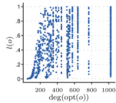
(a) ${\left|D\right|}=10^{3}$, $\rho=0.29$

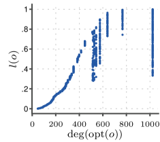
(b) ${\left|D\right|}=10^{4}$, $\rho=0.77$

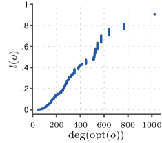
(c) ${\left|D\right|}=10^{5}$, $\rho=0.97$

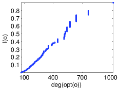
(d) ${\left|D\right|}=10^{6}$, $\rho=0.98$

Figure 2: Measure $l\mathopen{}\left(o\right)$ as a function of $\mathrm{deg}\mathopen{}\left(\mathrm{opt}\mathopen{}\left(o\right)\right)$, the number of free parameters. Theorem 7.1 implies that asymptotically $l\mathopen{}\left(o\right)$ is a monotonic function of $\mathrm{deg}\mathopen{}\left(\mathrm{opt}\mathopen{}\left(o\right)\right)$. Each plot contain $1000$ random orders of a dataset generated similarly as Path dataset. The number of transactions is indicated in each sublabel. The variable $\rho$ is the correlation between $l\mathopen{}\left(o\right)$ and $\mathrm{deg}\mathopen{}\left(\mathrm{opt}\mathopen{}\left(o\right)\right)$.

From the results given in Figure 2 we see that the measure $l\mathopen{}\left(o\right)$ converges into an increasing function of $\mathrm{deg}\mathopen{}\left(\mathrm{opt}\mathopen{}\left(o,p\right)\right)$ as the number of transactions increases. Note that for the first two datasets there are many orders which have the maximal number of free parameters, $1023$, yet their measure values are small. Such behavior is hinted by Proposition 4.1: In such orders the model $\mathrm{opt}\mathopen{}\left(o,p\right)$ is equal to one segment, containing all items. Proposition 4.1 states that the necessary condition to produce this model as the model with the lowest BIC score we must have an exponential number of transactions. Note that in the larger datasets we have enough transactions to convince us that the model with the worst BIC penalty term is actually the best.

8.3 Spectral Methods with Real Datasets

We continue our experiments with real-world datasets. The dataset Paleo contains information of species fossils found in specific paleontological sites in Europe [9]. The dataset Courses contains the enrollment records of students taking courses at the Department of Computer Science of the University of Helsinki. We took datasets Anneal and Mushroom from the LUCS/KDD repository [10]. A click-stream dataset WebView-1  was contributed by Blue Martini Software as the KDD Cup 2000 data [11]. The final dataset, Dna, is DNA copy number amplification data collection of human neoplasms [12]. Each dataset was split into two, the first part was used for calculating the order and the second part to calculate the actual score. To compute the measures we also computed the scores for $1000$ random orders. The basic characteristics and the running times are given in Table 2.

Name	$K$	${\left|D\right|}$	% of 1s	Time
Anneal	$73$	$898$	$20\%$	$3ms$
Courses	$98$	$3506$	$5\%$	$8ms$
Dna	$391$	$4587$	$1\%$	$24ms$
Mushroom	$90$	$8124$	$25\%$	$44ms$
Paleo	$139$	$501$	$5\%$	$3ms$
WebView-1	$497$	$59602$	$1\%$	$331ms$

Table 2: Statistics and running times of datasets used in experiments. The 4th column is the time needed to compute a score for one order.

Measure $l\mathopen{}\left(o\right)$ was $0$ for all orders and datasets, except for Anneal, where $l\mathopen{}\left(\textsc{CO}\right)=l\mathopen{}\left(\textsc{CS}\right)=0.03$. This suggests that the almost all found orders were significantly good. To illustrate this further we plotted the scores of the random and the spectral orders in a box plot in Figure 3.

Data	CO	CS	MI	M2
Anneal	$5.93$	$6.04$	$82.96$	$47.89$
Courses	$55.47$	$72.80$	$54.31$	$58.72$
Dna	$\infty$	$\infty$	$\infty$	$\infty$
Mushroom	$39.13$	$18.69$	$46.74$	$54.18$
Paleo	$129.39$	$109.39$	$13.18$	$131.01$
WebView-1	$289.08$	$229.18$	$561.93$	$764.20$

Table 3: Measure $r\mathopen{}\left(o\right)$ of the spectral orders obtained from the real datasets. The orders are explained in Section 5.1.

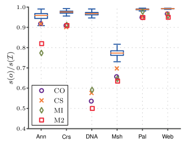
Figure 3: A box plot of the scores of random and spectral orders. The scores were normalized by dividing with $s\mathopen{}\left(\mathcal{I}\right)$, the score of the independent model.

Examining Table 3 reveals that the best scores are achieved with Dna dataset, suggesting that there is a strong order structure in the dataset. Measures $r\mathopen{}\left(o\right)$ becomes infinite due to the finite precision of the floating point number. Also, the scores of the spectral orders for the Mushroom dataset are small but so are the scores of the random orders. This implies that there are lot of dependencies in the dataset but the order structure is not that strong. Interestingly enough, either MI or M2 produces the lowest score for $5$ datasets. One possible explanation is that MI and M2 are able to use the negative correlations and their score is directly related to the log-likelihood of the model. On the other hand, the order CS is the best for the Courses dataset and the order MI fails with Paleo dataset.

8.4 Improving the Scores with Greedy Search

We conclude our experiments by studying the greedy method discussed in Section 5.2. We applied the algorithm for the first part of each dataset. As starting points we used the orders obtained by the spectral methods. Our hope is that the greedy method improves the scores of spectral order because it is able to use statistics of higher-order and because spectral orders are only guaranteed to work with $L$-matrices (see Section 5.1).

For comparison we sampled up to $50$ orders from the PQ-tree produced by Atkins’ algorithm. Each order was used as a starting point for the greedy algorithm. We also tested the greedy method with $50$ random starting orders. The obtained orders were then evaluated by computing the scores from the second part of the dataset. The running times varied from $1$ second to $1$ hour, depending on the size of the dataset.

Name	CO	CS	MI	M2	RND
Anneal	$5.05$	$3.39$	$2.98$	$3.25$	$3.41$
Courses	$2.50$	$2.02$	$1.56$	$2.82$	$1.68$
Dna	$7.36$	$9.26$	$12.57$	$8.80$	$2.31$
Mushroom	$7.28$	$9.18$	$9.91$	$13.33$	$7.66$
Paleo	$0.80$	$0.98$	$0.61$	$0.98$	$0.58$
WebView-1	$0.92$	$1.62$	$1.20$	$1.59$	$0.63$

Table 4: Gains of the scores when using the greedy method compared to the scores of the starting points. The percentages are computed as $100\%-100\%\times s\mathopen{}\left(o_{1}\right)/s\mathopen{}\left(o_{2}\right)$, where $o_{1}$ is the final order and $o_{2}$ is the starting order.

	$l\mathopen{}\left(o\right)$		$r\mathopen{}\left(o\right)$
Data	RND		CO	CS	MI	M2	RND
Anneal	$0.12$		$20.1$	$14.6$	$104.2$	$66.9$	$2.9$
Courses	$0.10$		$100.3$	$110.9$	$79.8$	$109.8$	$3.4$
Dna	$0.03$		$\infty$	$\infty$	$\infty$	$\infty$	$4.9$
Mushroom	$0.01$		$75.2$	$56.1$	$100.9$	$136.1$	$7.5$
Paleo	$0.13$		$181.5$	$169.7$	$26.9$	$196.3$	$2.8$
WebView-1	$0$		$453.7$	$570.5$	$871.4$	$940.0$	$11.6$

Table 5: Measures $l\mathopen{}\left(o\right)$ and $r\mathopen{}\left(o\right)$ of the orders obtained using the greedy method with the spectral and random orders as the starting points. Measure values $l\mathopen{}\left(o\right)$ for all spectral orders were $0$ and are omitted from the table.

By comparing the measure $r\mathopen{}\left(o\right)$ given in Table 5 to the values given in Tables 3 we see that the greedy method does not perform well alone: when random orders are used as starting points, the discovered orders are worse than the spectral orders. However, greedy method is useful when spectral orders are used as starting points. From Table 4 we see that the greedy method improves the scores of the spectral orders up to $13$ percents. The gain of the score depends on the dataset but less on the spectral method used. The scores for Courses, Paleo and WebView-1 datasets improve up to $3$ percents where as the biggest gains are with Dna, and Mushroom datasets where the scores improve by $7$ – $13$ percents.

9 Related Work

A popular choice for measuring the goodness of an order is the Lazarus count, the number of $0$s between $1$s in a row. If the Lazarus count is $0$, then the data is said to have the consecutive ones property. In some cases this has a natural interpretation, for example, in a paleontological data a taxon becomes extant and then extinct. If the matrix has a consecutive ones property, then the Fiedler vector of the co-occurrence matrix returns the correct order [8]. It is an open question why the spectral method works also with the noisy data. An alternative approach has been suggested in [13], where the authors construct a probabilistic model encapsulating the consecutive ones property.

Ranking or sorting items can be seen as deducing a linear order for the items. Applications for ranking are, for example, finding relevant web pages [14, 15] or ranking database query results [16]. One of the key differences in these approaches and ours is that in our case the reversed order is as good as the original. We are interested in finding the order in which the dependent attributes are close. This goal is different than finding the most relevant items.

In some cases, linear orders is too strict a structure, in such case partial orders (transitive, asymmetric, and reflexive relation) may be more natural. For example, consider the course enrollment data, in which the same basic course is prerequisite for several advanced independent courses. Finding partial orders have been studied for example in [17]. General partial orders seem to be very complex objects. A simple but yet interesting subclass of partial orders are bucket orders [18, 16]. A problem of searching fragments of order, that is finding a collection of linear orders defined for a subset of items has been studied in [19].

10 Conclusions

We studied the concept of measuring the goodness of an order. We say that the order is good if the heavily dependent attributes are close to each other. In order to define the score we introduce an order-sensitive model and then use the BIC score to rank the model. To find the optimal model we created a dynamic program and show that it can be evaluated in $O\mathopen{}\left(K\min\mathopen{}\left(K,\log{\left|D\right|}\right)^{2}\right)$ time. Hence, our method works well even for the datasets with vast number of items.

We provided asymptotic results showing that the score is connected the number of free parameters in the model. We also demonstrate this result empirically with synthetic data.

We compared the score of the order against the scores of random orders. We say that the order is good if the score is exceptionally lower than the score of the random order. We used two different measures, $l\mathopen{}\left(o\right)$ the proportion of random scores having the smaller score than $o$, and $r\mathopen{}\left(o\right)$, the ratio of the score $s\mathopen{}\left(o\right)$ and the average score of a random order. One of our future goals is to develop a more refined measure for comparing the score against the scores of random orders.

We evaluate the measures with several spectral and greedy methods. In our experiments we found out that Fiedler orders of the mutual information matrices (see Section 5.1) produced better results for our datasets than the orders based on co-occurrences or cosine distance. In our experiments, the greedy optimization improved the scores of spectral orders up to $13$ percents.

One of our future goals is to extend the current method for more general partial orders (see Section 9). Such an extension is not trivial since in general case finding the best model is a computationally difficult task.

A Proof of Theorem 7.1

Throughout the whole section we will assume that the underlying distribution $p$ has no zero probabilities, $p>0$.

Given a distribution $q$ and a set of segments $\mathcal{C}$ we will adopt the notation $h(A=t)=q(A=t;\mathcal{C})$ to mean the unique distribution $h\in M\mathopen{}\left(\mathcal{C}\right)$ such that $q(C)=h(C)$ for any $C\in\mathcal{C}$.

We begin by considering indicator functions. Given an itemset $X=\left\{a_{i_{1}},\ldots,a_{i_{L}}\right\}$ we define an indicator function ${S_{X}}:{\left\{0,1\right\}^{K}}\to{\left\{0,1\right\}}$ to be $S_{X}(t)=t_{i_{1}}\cdots t_{i_{L}}$. Thus $S_{X}(t)=1$ if and only if all $t_{i}$ corresponding to the elements of $X$ have value of 1. We also define $S_{\emptyset}(t)=1$.

Lemma A.1

Given a family of itemsets $\mathcal{X}$, the set of indicator functions $\mathcal{S}=\left\{S_{X};X\in\mathcal{X}\right\}$ are independent, that is, $\sum_{X\in\mathcal{X}}r_{X}S_{X}(t)=0$ is possible only for $r_{X}=0$. If $\mathcal{X}$ contains all itemsets, then $\mathcal{S}$ forms a basis.

• It is sufficient to prove the lemma for the case when $\mathcal{X}=\left\{X;X\in A\right\}$ contains all possible itemsets.

  For a $v\in\left\{0,1\right\}^{K}$, Consider a function ${T_{v}}:{\left\{0,1\right\}^{K}}\to{\left\{0,1\right\}}$ for which $T_{v}(t)=1$ if and only if $t=v$. Obviously, the set of functions $\mathcal{T}=\left\{T_{v};v\in\left\{0,1\right\}^{K}\right\}$ is linearly independent. Hence to prove the lemma we need to show that we can build a linear mapping from $\mathcal{T}$ onto $\mathcal{S}$ that has an inverse.

  To prove this we first note that $S_{X}(t)=\sum_{Y\supseteq X}T_{Y}(t)$. This can be inverted using the inclusion-exclusion principle $T_{X}(t)=\sum_{Y\supseteq X}(-1)^{{\left|Y\right|}-{\left|X\right|}}S_{Y}(t)$. This completes the proof.

A direct calculation implies that the distributions in $M\mathopen{}\left(\mathcal{C}\right)$ have a particular exponential form.

Lemma A.2

Let $\mathcal{X}=\left\{X;X\subseteq C\in\mathcal{C}\right\}$ be the downward closure of $\mathcal{C}$. A distribution $p$ is in $M\mathopen{}\left(\mathcal{C}\right)$ if only if $p(A=t)=\exp\mathopen{}\left(\sum_{X\in\mathcal{X}}r_{X}S_{X}(t)\right)$ for some specific constants $\left\{r_{X}\right\}$.

• Assume that $p\in M\mathopen{}\left(\mathcal{C}\right)$. Then $p$ has a form of $p(A)=\prod p\mathopen{}\left(C_{i}\right)/\prod p\mathopen{}\left(C_{i}\cap C_{i-1}\right)$. Fix $i$. Lemma A.1 now implies that we can write $\log p\mathopen{}\left(C_{i}=t_{C_{i}}\right)=\sum_{X\subseteq C_{i}}a_{X}S_{X}(t)$ or in other words $p\mathopen{}\left(C_{i}=t_{C_{i}}\right)=\exp\mathopen{}\left(\sum_{X\subseteq C_{i}}a_{X}S_{X}(t)\right)$. We can perform this factorization for each $p(C_{i})$ and for each $p\mathopen{}\left(C_{i}\cap C_{i-1}\right)$. By combining these factorizations we arrive at the desired result.

  We will prove the other direction by induction. Let $p$ be the distribution having the exponential form and let $\left\{r_{X}\right\}$ be the needed constants. Shorten $V=C_{1}$, $W=A-(C_{1}-C_{2})$, and $H=C_{1}\cap C_{2}$.

  Using the argument in the first paragraph we can write $p\mathopen{}\left(H=t_{H}\right)=\exp\mathopen{}\left(\sum_{X\subseteq H}u_{X}S_{X}(t)\right)$ for some constants $\left\{u_{X}\right\}$. Note that if $X\in\mathcal{X}$ is such that $X\nsubseteq H$, then either $X\subseteq V$ or $X\subseteq W$. We have

  $$\begin{split}&\log p\mathopen{}\left(A-H=t_{A-H}\mid H=t_{H}\right)\\ &\quad=\sum_{X\in\mathcal{X}}r_{X}S_{X}(t)-\sum_{X\in\mathcal{X},X\subseteq H}u_{X}S_{X}(t)\\ &\quad=\sum_{X\in\mathcal{X},X\subseteq V}r_{X}S_{X}(t)+\sum_{X\in\mathcal{X},X\subseteq W}r_{X}S_{X}(t)\\ &\qquad-\sum_{X\in\mathcal{X},X\subseteq H}(r_{X}+u_{X})S_{X}(t).\end{split}$$

  The third term depends only on $t_{H}$, hence it is a part of the normalization constant of the conditioned distribution. The first term depends only on the values of $t_{V}$ while the second term depends only on the values of $t_{W}$. This leads to

  $$\begin{split}p(A)&=p(A-H\mid H)p(H)\\ &=p(V-H\mid H)p(W-H\mid H)p(H)\\ &=\frac{p(V)p(W)}{p(H)}=\frac{p(C_{1})p(W)}{p(C_{1}\cap C_{2})}.\end{split}$$

  The distribution $p(W)=p(W\mid H)p(H)$ has an exponential form, hence if we assume inductively that $p(W)\in M\mathopen{}\left(\mathcal{C}-C_{1}\right)$, then the above equality proves that $p(A)\in M\mathopen{}\left(\mathcal{C}\right)$.

Our next step is to study $\mathrm{opt}\mathopen{}\left(o,p\right)$. Let $\mathcal{V},\mathcal{W}\in\mathrm{seg}\mathopen{}\left(o\right)$. We say that $\mathcal{W}$ refines $\mathcal{V}$ if for each $V\in\mathcal{V}$ there is $W\in\mathcal{W}$ such that $V\subseteq W$. In this case we write $\mathcal{V}\sqsubset\mathcal{W}$. We will now show that $\mathrm{opt}\mathopen{}\left(o,p\right)$ is the minimal set with the respect of the relation $\sqsubset$.

Theorem A.1

Let $\mathcal{O}=\mathrm{opt}\mathopen{}\left(o,p\right)$. If $\mathcal{C}$ is such that $p\in M\mathopen{}\left(\mathcal{C}\right)$, then $\mathcal{O}\sqsubset\mathcal{C}$. Moreover, $\mathcal{O}$ is unique.

• Assume otherwise and define $\mathcal{V}$ to be the maximal segments of the set of segments $\left\{C\cap O;C\in\mathcal{C},O\in\mathcal{O}\right\}$. Clearly $\mathrm{deg}\mathopen{}\left(\mathcal{V}\right)<\mathrm{deg}\mathopen{}\left(\mathcal{O}\right)$. We need to show that $p\in M\mathopen{}\left(\mathcal{V}\right)$. Let $\mathcal{X}$ and $\mathcal{Y}$ be the downward closure of $\mathcal{O}$ and $\mathcal{C}$, respectively. Let $\left\{r_{X}\right\}$, $\left\{s_{Y}\right\}$ be the sets of constants in Lemma A.2 when applied to $\mathcal{X}$ and $\mathcal{Y}$, respectively. We have

  $$\sum_{X\in\mathcal{X}}r_{X}S_{X}(t)=\log p(A=t)=\sum_{Y\in\mathcal{Y}}s_{Y}S_{Y}(t).$$

  Since the functions $S_{X}$ are linearly independent we must have that $r_{Z}=s_{Z}$ for any $Z\in\mathcal{X}\cap\mathcal{Y}$ and $r_{X}=0$, $s_{Y}=0$ otherwise. The downward closure of $\mathcal{V}$ is exactly $\mathcal{X}\cap\mathcal{Y}$. But now Lemma A.2 implies that $p\in M\mathopen{}\left(\mathcal{V}\right)$ which is a contradiction by the minimality of $\mathcal{O}$.

We will need the following technical lemma that states that the difference between the likelihood terms is bounded.

Lemma A.3

Assume two orders $o_{1}$ and $o_{2}$. Let $\mathcal{O}_{i}=\mathrm{opt}\mathopen{}\left(o_{i},p\right)$ and let $\mathcal{C}_{i}\in\mathrm{seg}\mathopen{}\left(o_{i}\right)$ such that $\mathcal{O}_{i}\sqsubset\mathcal{C}_{i}$. Let $D$ be a dataset with $N={\left|D\right|}$ transactions and let $h_{i}=q_{D}\left(A;\mathcal{C}_{i}\right)\in M\mathopen{}\left(\mathcal{C}_{i}\right)$. Let $Z_{N}=NH\mathopen{}\left(h_{1}\right)-NH\mathopen{}\left(h_{2}\right)$ and let $Z$ be the limit distribution as $N\to\infty$. Then $P(Z_{N}<t)\to P(Z<t)$ uniformly in $t$ as $N\to\infty$. Moreover, $P(Z=\infty)=0$.

• Let $\mathcal{X}_{i}$ be the downward closure of $\mathcal{O}_{i}$ and let $\left\{r^{i}_{O}\right\}$ be the set of constraints given by Lemma A.2 when applied to $\mathcal{O}_{i}$ and $p$. Note that we have

  $$\sum_{O\in\mathcal{X}_{1}}r^{1}_{O}S_{O}(t)=\log p(A=t)=\sum_{O\in\mathcal{X}_{2}}r^{2}_{O}S_{O}(t).$$

  Since the functions $S_{O}$ are linearly independent we must have $r^{1}_{O}=r^{2}_{O}$ whenever $O\in\mathcal{X}_{1}\cap\mathcal{X}_{2}$ and $r^{i}_{O}=0$ otherwise.

  Let $\mathcal{Y}=\mathcal{X}_{1}\cap\mathcal{X}_{2}$. We know that (see Theorem 3.1 in [20]) there is a set of constants $\left\{r_{Y}\right\}$ such that the distribution $g$ defined as $g(A=t)=\exp\mathopen{}\left(\sum_{Y\in\mathcal{Y}}r_{Y}S_{Y}(t)\right)$ has the property $g(S_{Y}=1)=q_{D}(S_{Y}=1)$. Now a classic result (see [21] for example) implies that $NH\mathopen{}\left(h_{i}\right)-NH\mathopen{}\left(g\right)$ converges into a chi-square distribution. A known result (see Theorem 2.3 in [22]) implies that the distribution of $Z$ is a difference of two chi-square distributions implying that $P(Z=\infty)=0$. Since $Z$ is continuous, a known result (see Lemma 2.11 in vaart98statistics) now implies that the convergence is uniform.

Elementary analysis now implies the following key corollary.

Corollary A.1

Let $Z_{N}$ as in Lemma A.3 and let $t_{N}$ be a sequence such that $t_{N}\to\infty$. Then $P\mathopen{}\left(Z_{N}\geq t_{N}\right)\to 0$.

Let $D$ be a dataset with $N$ transactions. We will denote by $\mathcal{C}^{N}\in\mathrm{seg}\mathopen{}\left(o\right)$ to be the model with the lowest score. Note that $\mathcal{C}^{N}$ is a random variable since it depends on $D$. We will show that $\mathcal{C}^{N}$ converges into $\mathrm{opt}\mathopen{}\left(o,p\right)$.

Theorem A.2

Let $\mathcal{O}=\mathrm{opt}\mathopen{}\left(o,p\right)$. Then $P\left(\mathcal{O}=\mathcal{C}^{N}\right)\to 1$ as $N$ approaches infinity.

• Let $\mathcal{C}\in\mathrm{seg}\mathopen{}\left(o\right)$ such that $\mathcal{O}\not\sqsubset\mathcal{C}$. Let $h=p(A;\mathcal{C})\in M\mathopen{}\left(\mathcal{C}\right)$. Theorem A.1 now implies that $h\neq p$. Note that

  $$\begin{split}\lim_{N}\frac{s\mathopen{}\left(\mathcal{C}\right)}{N}&=-\sum_{t}p(A=t)\log h(A=t)\\ &>H\mathopen{}\left(p\right)=\lim_{N}\frac{s\mathopen{}\left(\mathcal{O}\right)}{N}.\end{split}$$

  Hence $P\left(\mathcal{C}=\mathcal{C}^{N}\right)\to 0$ since $\mathcal{C}^{N}$ is the collection of segments with the optimal score.

  Assume now that $\mathcal{O}\sqsubset\mathcal{C}$, $\mathcal{O}\neq\mathcal{C}$. Let $h=q_{D}\mathopen{}\left(A;\mathcal{O}\right)$ and $g=q_{D}\mathopen{}\left(A;\mathcal{C}\right)$. Set $d=1/2(\mathrm{deg}\mathopen{}\left(\mathcal{C}\right)-\mathrm{deg}\mathopen{}\left(\mathcal{O}\right))$. Note that

  $$s\mathopen{}\left(\mathcal{O}\right)-s\mathopen{}\left(\mathcal{C}\right)=NH\mathopen{}\left(h\right)-NH\mathopen{}\left(g\right)-d\log N.$$

  Since $d\log N\to\infty$ as $N\to\infty$, Corollary A.1 implies that

  $$P\mathopen{}\left(s\mathopen{}\left(\mathcal{O}\right)\geq s\mathopen{}\left(\mathcal{C}\right)\right)=P\mathopen{}\left(NH\mathopen{}\left(h\right)-NH\mathopen{}\left(g\right)\geq d\log N\right)\to 0.$$

  Thus we must have $P\left(\mathcal{O}=\mathcal{C}^{N}\right)\to 1$.

We are now ready to prove the main theorem.

• [of Theorem 7.1] The theorem follows if we can prove that $s\mathopen{}\left(o_{1}\right)$ is lower than $s\mathopen{}\left(o_{2}\right)$ with probability $1$ as $N$ approaches infinity. Let $\mathcal{O}_{i}=\mathrm{opt}\mathopen{}\left(o_{i},p\right)$. We write

  $$\begin{split}&P\left(s\mathopen{}\left(o_{1}\right)\geq s\mathopen{}\left(o_{2}\right)\right)\\ &\quad\leq P\left(s\mathopen{}\left(\mathcal{O}_{1}\right)\geq s\mathopen{}\left(\mathcal{O}_{2}\right)\right)+P\left(\mathcal{C}^{N}_{1}\neq\mathcal{O}_{1}\lor\mathcal{C}^{N}_{2}\neq\mathcal{O}_{2}\right)\\ &\quad\leq P\left(s\mathopen{}\left(\mathcal{O}_{1}\right)\geq s\mathopen{}\left(\mathcal{O}_{2}\right)\right)+P\left(\mathcal{C}^{N}_{1}\neq\mathcal{O}_{1}\right)+P\left(\mathcal{C}^{N}_{2}\neq\mathcal{O}_{2}\right).\end{split}$$

  Theorem A.2 implies that the second and the third terms converge to 0. To annihilate the first term we use again Corollary A.1. Let $g_{i}=q_{D}\mathopen{}\left(A;\mathcal{O}_{i}\right)$. Set $d=1/2(\mathrm{deg}\mathopen{}\left(\mathcal{O}_{2}\right)-\mathrm{deg}\mathopen{}\left(\mathcal{O}_{1}\right))$. Note that

  $$s\mathopen{}\left(\mathcal{O}_{1}\right)-s\mathopen{}\left(\mathcal{O}_{2}\right)=NH\mathopen{}\left(g_{1}\right)-NH\mathopen{}\left(g_{2}\right)-d\log N.$$

  Since $d\log N\to\infty$ as $N\to\infty$, Corollary A.1 implies that

  $$\begin{split}&P\mathopen{}\left(s\mathopen{}\left(\mathcal{O}_{1}\right)\geq s\mathopen{}\left(\mathcal{O}_{2}\right)\right)\\ &\quad=P\mathopen{}\left(NH\mathopen{}\left(g_{1}\right)-NH\mathopen{}\left(g_{2}\right)\geq d\log N\right)\to 0.\end{split}$$

  This completes the proof.

References

- [1] M. Fortelius, A. Gionis, J. Jernvall, and H. Mannila, “Spectral ordering and biochronology of european fossil mammals,” Paleobiology, vol. 32, no. 2, pp. 206–214, March 2006.
- [2] D. G. Kendall, “Abundance matrices and seriation in archaeology,” Probability Theory and Related Fields, vol. 17, no. 2, pp. 104–112, June 1971.
- [3] A. Gionis, H. Mannila, and J. K. Seppänen, “Geometric and combinatorial tiles in 0-1 data,” in 8th European Conference on Principles and Practice of Knowledge Discovery in Databases (PKDD 2004), 2004, pp. 173–184.
- [4] R. G. Cowell, A. P. Dawid, S. L. Lauritzen, and D. J. Spiegelhalter, Probabilistic Networks and Expert Systems, ser. Statistics for Engineering and Information Science, M. Jordan, S. L. L. nad Jeral F. Lawless, and V. Nair, Eds. Springer-Verlag, 1999.
- [5] G. Schwarz, “Estimating the dimension of a model,” Annals of Statistics, vol. 6, no. 2, pp. 461–464, 1978.
- [6] C. H. Papadimitriou, Computational Complexity. Addison-Wesley, 1994.
- [7] M. Fiedler, “A property of eigenvectors of nonnegative symmetric matrices and its application to graph theory,” Czechoslovak Mathematical Journal, vol. 25, no. 4, pp. 619–633, 1975.
- [8] J. E. Atkins, E. G. Boman, and B. Hendrickson, “A spectral algorithm for seriation and the consecutive ones problem,” SIAM J. Comput., vol. 28, no. 1, pp. 297–310, 1999.
- [9] M. Fortelius, “Neogene of the old world database of fossil mammals (NOW),” University of Helsinki, http://www.helsinki.fi/science/now/, 2005.
- [10] F. Coenen, “The LUCS-KDD discretised/normalised ARM and CARM data library,” 2003.
- [11] R. Kohavi, C. Brodley, B. Frasca, L. Mason, and Z. Zheng, “KDD-Cup 2000 organizers’ report: Peeling the onion,” SIGKDD Explorations, vol. 2, no. 2, pp. 86–98, 2000.
- [12] S. Myllykangas, J. Himberg, T. B hling, B. Nagy, J. Hollmén, and S. Knuutila, “Dna copy number amplification profiling of human neoplasms,” Oncogene, vol. 25, no. 55, pp. 7324–7332, Nov. 2006.
- [13] K. Puolamäki, M. Fortelius, and H. Mannila, “Seriation in paleontological data using markov chain monte carlo methods,” PLoS Comput Biol, vol. 2, no. 2, Feb 2006. [Online]. Available: http://dx.doi.org/10.1371%2Fjournal.pcbi.0020006
- [14] S. Brin and L. Page, “The anatomy of a large-scale hypertextual web search engine,” Computer Networks and ISDN Systems, vol. 30, no. 1–7, pp. 107–117, 1998.
- [15] J. Kleinberg, “Authoritative sources in a hyperlinked environment,” Journal of the ACM, vol. 46, no. 5, pp. 604–632, 1999.
- [16] R. Fagin, R. Kumar, M. Mahdian, D. Sivakumar, and E. Vee, “Comparing and aggregating rankings with ties,” in Proceedings of the ACM-SIAM Symposium on Discrete Algorithms (PODS), 2004, pp. 47–58.
- [17] A. Ukkonen, M. Fortelius, and H. Mannila, “Finding partial orders from unordered 0-1 data,” in KDD ’05: Proceedings of the eleventh ACM SIGKDD international conference on Knowledge discovery in data mining. New York, NY, USA: ACM, 2005, pp. 285–293.
- [18] A. Gionis, H. Mannila, K. Puolamäki, and A. Ukkonen, “Algorithms for discovering bucket orders from data,” in KDD ’06: Proceedings of the 12th ACM SIGKDD international conference on Knowledge discovery and data mining. New York, NY, USA: ACM, 2006, pp. 561–566.
- [19] A. Gionis, T. Kujala, and H. Mannila, “Fragments of order,” in KDD ’03: Proceedings of the ninth ACM SIGKDD international conference on Knowledge discovery and data mining. New York, NY, USA: ACM, 2003, pp. 129–136.
- [20] I. Csiszár, “I-divergence geometry of probability distributions and minimization problems,” The Annals of Probability, vol. 3, no. 1, pp. 146–158, Feb. 1975.
- [21] A. Wald, “Tests of statistical hypotheses concerning several parameters when the number of observations is large,” Trans. of the American Mathematical Society, vol. 54, no. 3, pp. 426–482, Nov. 1943.
- [22] A. W. van der Vaart, Asymptotic Statistics, ser. Cambridge Series in Statistical and Probabilistic Mathematics. Cambridge University Press, 1998.