Complete Glauber calculations for proton-nucleus inelastic cross sections

Abstract

We perform a parameter-free calculation for the high-energy proton-nucleus scattering based on the Glauber theory. A complete evaluation of the so-called Glauber amplitude is made by using the factorization of the single-particle wave functions. The multiple-scattering or multistep processes are fully taken into account within the Glauber theory. We demonstrate that proton-¹²C, ²⁰Ne, and ²⁸Si elastic and inelastic scattering ($J^{\pi}=0^{+}\to 2^{+}$ and $0^{+}\to 4^{+}$) processes are very well described in a wide range of the incident energies from $\sim 50$ MeV to $\sim 1$ GeV. We evaluate the validity of a simple one-step approximation and find that the approximation works fairly well for the inelastic $0^{+}\to 2^{+}$ processes but not for $0^{+}\to 4^{+}$ where the multistep processes become more important. As an application, we quantify the difference between the total reaction and interaction cross sections of proton-¹²C, ²⁰Ne, and ²⁸Si collisions.

1 Introduction

Recent major upgrades in radioactive beam facilities provide the platform to study the exotic phenomena in the unstable nuclei far from the stability line. The understanding of the role of the excess neutrons in isotopic chains has been deepened through the studies of the nuclear excitations using exotic radioactive-ion beams, for example, a systematic measurement of quadrupole transition strengths has shown anomalous structure changes due to neutron excess in the neutron-rich carbon isotopes  [1, 2, 3, 4].

Since short-lived nuclei cannot be used as a target nucleus, the nuclear direct reactions in the inverse kinematics have often been utilized as a tool to study the structure of such nuclei. A proton, which is the simplest probe, has often been used to populate the excited states of nuclei. Thanks to high-intensity radioactive beams, the proton inelastic scattering cross section measurements of the short-lived nuclei have become possible with use of the inverse kinematics. [5, 6, 7]. In contrast to electron and photon scattering, both proton and neutron parts of the projectile nucleus can directly be excited through the proton inelastic scattering processes. This is advantageous for studying the detailed structure of the neutron-rich nuclei where the neutron excitations are expected to be dominant. Here we focus on the proton-nucleus inelastic scattering at about 50 to the several hundred MeV where the measurements have often been made. This high-energy region is beneficial for a theoretical description as the reaction mechanism is much simpler than the low-energy region in which the complicated channel coupling effects should be taken into account [8].

Towards the future measurements of the inelastic scattering cross sections for unstable nuclei, in this paper, we develop a parameter-free reaction theory based on the Glauber theory [9] and test it in comparison to the available experimental data. The Glauber theory is one of the most widely accepted methods to describe the nuclear reactions at high incident energies. We evaluate proton-nucleus inelastic scattering cross sections following the original Glauber theory which includes all multiple-scattering or multistep processes within the eikonal and adiabatic approximations. According to the original formulation of the Glauber theory, the inputs to the theory are wave functions (not one-body densities) of the colliding nuclei and the so-called profile function parametrized based on the total nucleon-nucleon cross section. Therefore, the theory includes no adjustable parameter. Most complicated part of the computation is the evaluation of the so-called Glauber amplitude involving multidimensional integration, which is in general difficult, and often approximate treatment has been made to avoid that difficulty. By introducing appropriate approximations, the theory successfully reproduced the observed cross sections of the unstable nuclei and revealed the evolution of the nuclear deformation in the neutron-rich isotopes [10, 11]. However, the complete and approximated Glauber amplitudes significantly deviate in case of halo nuclei where the nuclear surface is very much extended [12, 13, 14, 15]. Since the inelastic scattering occurs mainly around the nuclear surface, the complete evaluation of the Glauber amplitude which includes all the multistep processes in the Glauber theory will be necessary for a more reliable description of the scattering processes.

The purpose of this paper is to establish a reliable microscopic framework following the original Glauber theory towards future proton-nucleus inelastic cross section measurements involving the exotic nuclei. We remark that Ref. [16] reported the complete Glauber calculations for proton-¹²C inelastic scattering cross sections and successfully reproduced the cross sections at $\sim$1 GeV. However, the form of the wave function they used is limited to an analytically integrable form such as harmonic-oscillator wave functions in which applications to heavier nuclei as well as extension to more general wave function is difficult. In the present study, we extend this approach in order to use more general forms of the wave functions. To demonstrate the power of this approach, we systematically analyze the inelastic scattering cross sections for well known nuclei ¹²C, ²⁰Ne, and ²⁸Si, and compare them with the available experimental data.

The paper is organized as follows. In Sec. 2, we briefly explain the Glauber theory to describe the nuclear elastic and inelastic processes. In Sec. 2.1, the formulation to compute these cross sections is given based on the Glauber multiple-scattering theory. Sec. 2.2 explains how we evaluate the complete Glauber amplitude for the elastic and inelastic scattering cross section calculations. For later use, approximate formulation to evaluate the Glauber amplitude is given in Sec. 2.3. This theory will be tested for the evaluation of the elastic and inelastic cross sections of ¹²C, ²⁰Ne, and ²⁸Si. Though the theory can use any type of the single-particle wave functions, we, however, employ deformed harmonic-oscillator wave functions for the sake of simplicity which are defined in Sec. 2.4. Section 3 discusses our results of the elastic and inelastic scattering cross sections. We show the physical properties of our wave functions in Sec. 3.1. Section 3.2 compares the theoretical elastic and inelastic scattering cross sections with the available cross section data. The approximate methods are also tested in this section in order to quantify the importance of the multiple-scattering or multistep processes which have often been neglected. The structure of ²⁸Si is discussed through a systematic analysis of the inelastic scattering cross sections. The energy dependence of the inelastic scattering processes is discussed in Sec. 4. As an application of this theory, in Sec. 5, we evaluate difference between the total reaction and interaction cross sections as they impacts on the accuracy of the radius extraction from the measured interaction cross section. A summary is given in Sec. 6. More details about the evaluation of the Glauber amplitude are described in Appendices A and B.

2 Theoretical models

The Glauber theory [9] is a powerful tool to describe the scattering processes in high-energy nucleus-nucleus collisions. In this section, we summarize how the scattering cross sections are evaluated with the Glauber theory. The Glauber amplitude is a key to the calculation of all the cross sections. Here we explain a procedure to compute it for proton-nucleus scattering.

2.1 Inelastic scattering cross sections within the Glauber theory

We consider the normal kinematics throughout this paper in which a high-energy proton is bombarded on a target nucleus for the sake of convenience, and assume that this incoming proton is not polarized. In the Glauber theory, the final state wave function of a proton and mass number $A$ system, $\Phi_{f}$, is greatly simplified with the help of the adiabatic and eikonal approximations as [9]

$$\Phi_{f}=\left[\prod_{j=1}^{A}e^{i\chi_{pN}({\bm{b}-\hat{\bm{s}}_{j}})}\right]\Phi_{0},$$ (1)

in which $\Phi_{f}$ is expressed by the product of the initial-(ground-)state wave function, $\Phi_{0}$, and the product of the proton-nucleon ($pN;N=p$ or $n$ for proton or neutron) phase-shift functions $e^{i\chi_{pN}(\bm{b}-\hat{\bm{s}}_{j})}$ with $\hat{\bm{s}}_{j}$ being the two-dimensional single-particle coordinate operator of the $j$th nucleon perpendicular to the beam direction $z$. We conveniently define the Glauber multiple-scattering operator as

$$\prod_{j=1}^{A}e^{i\chi_{pN}({\bm{b}-\hat{\bm{s}}_{j}})}=\prod_{j=1}^{A}\left[1-\Gamma_{pN}(\bm{b}-\hat{\bm{s}}_{j})\right]=\prod_{j=1}^{A}\mathcal{O}_{j}(\bm{b})$$ (2)

with the $pN$ profile function, $\Gamma_{pN}(\bm{b})$, which is usually parametrized as [17]

$$\Gamma_{pN}(\bm{b})=\frac{1-i\alpha_{pN}}{4\pi\beta_{pN}}\sigma_{pN}^{\rm tot}\exp\left[-\frac{\bm{b}^{2}}{2\beta_{pN}}\right],$$ (3)

where $\sigma_{pN}^{\rm tot}$, $\alpha_{pN}$, and $\beta_{pN}$ are the total $pN$ cross section, the ratio between the real and imaginary parts of the scattering amplitude at the forward angle, and the slope parameter, respectively. These parameter sets for various incident energies are taken from Ref. [18]. The validity of the profile function has been confirmed in a number of examples, not only for nucleon-nucleus scattering but also nucleus-nucleus scattering [19, 20, 10, 21, 22, 15], and thus the profile function in Ref. [18] can be regarded as one optimal choice, although there are some ambiguity due to the experimental uncertainty, especially at the low incident energies [18]. In the incident energies below the pion production threshold, the nucleon-nucleon elastic scattering differential cross sections obtained from a realistic nucleon-nucleon interaction will be useful to reduce the uncertainty of the profile function fixed by the data fitting. This is interesting and worth investigating in the future.

The scattering amplitude from the initial ground state $(\alpha=0)$ to the final state labeled with $\alpha$ can be calculated by [9, 23]

$$f_{\alpha}(q) =\frac{k}{2\pi i}\int d\bm{b}\,e^{i\bm{q}\cdot\bm{b}}\left[\delta_{\alpha,0}-\left<\Phi_{\alpha}\right|\prod_{j=1}^{A}\mathcal{O}_{j}(\bm{b})\left|\Phi_{0}\right>\right],$$ (4)

where $k$ is the wave number in the relativistic kinematics, $\bm{q}$ is the momentum transfer vector being $|\bm{q}|=q=2k\sin(\theta/2)$ with the scattering angle $\theta$ in the center-of-mass (cm) system. The orthogonormality relation $\left<\Phi_{\alpha}|\Phi_{0}\right>=\delta_{\alpha,0}$ is used in this derivation. In Appendix A, we give more details about the evaluation of Eq. (4).

The elastic $(\alpha=0)$ and inelastic $(\alpha\neq 0)$ scattering differential cross sections can be evaluated by

$$\frac{d\sigma_{\alpha}}{d\Omega}=\frac{v_{\alpha}}{v_{0}}|f_{\alpha}(q)|^{2},$$ (5)

where $v_{0}$ and $v_{\alpha}$ are the velocities of the initial-incoming and final-outgoing waves, respectively. In the adiabatic approximation, $v_{\alpha}/v_{0}$ is unity. This is reasonable when the beam energy is high enough as compared to the excitation energy of the nucleus. The inelastic scattering cross section can directly be obtained by integrating the differential cross sections over the scattering angles with $\alpha\neq 0$

$$\sigma_{\alpha} =\int d\Omega\,\frac{d\sigma_{\alpha}}{d\Omega}=\int d\bm{b}\,|\left<\Phi_{\alpha}\right|\prod_{j=1}^{A}\mathcal{O}_{j}(\bm{b})\left|\Phi_{0}\right>|^{2}.$$ (6)

It can be rewritten in terms of the so-called Glauber amplitude for the inelastic processes

$$\mathcal{T}_{\alpha}(J_{0}M_{0}\to J_{\alpha}M_{\alpha};\bm{b})=\left<\Phi_{\alpha;J_{\alpha}M_{\alpha}}\right|\prod_{j=1}^{A}\mathcal{O}_{j}(\bm{b})\left|\Phi_{0;J_{0}M_{0}}\right>,$$ (7)

where $J_{0}M_{0}$ $(J_{\alpha}M_{\alpha})$ is the the initial (final) angular momentum and its projection. The inelastic scattering cross section is evaluated by the expression

$$\sigma_{\rm\alpha}=\frac{1}{2J_{0}+1}\sum_{M_{0},M_{\alpha}}\int d\bm{b}\,\left|\mathcal{T}_{\alpha}(J_{0}M_{0}\to J_{\alpha}M_{\alpha};\bm{b})\right|^{2}.$$ (8)

2.2 Evaluation of the complete Glauber amplitude for the inelastic scattering

Evaluation of the Glauber amplitude of Eq. (7) requires in general the tedious computations as one has to evaluate the $A$-fold multidimensional integration. A Monte Carlo technique was successfully applied to evaluate the multidimensional integration [24, 15]. However, it cannot be applied to the inelastic scattering problem because the initial and final states are orthogonal in which the guiding function $\Phi_{\alpha}^{*}\Phi_{0}$ for the Metropolis algorithm [25] is no longer positive definite.

In the present work, we take another approach based on the idea presented in Ref. [26]. With use of a Slater determinant wave function, the Glauber amplitude is factorized and its multidimensional integration is reduced to the three-dimensional one on the single-particle coordinate, which can simply be evaluated by a standard numerical integration technique, e.g., the trapezoidal rule and the Gaussian quadrature. This factorization technique has been successfully applied to realistic proton-nucleus elastic scattering of various nuclear systems [19, 27, 28]. In order to apply this method to the proton-nucleus inelastic scattering computation, here we extend the expression in order to use the wave function expressed by multi-Slater determinants. An earlier study was done for the proton-¹²C inelastic scattering with a specific form of the wave function [16]. Here we generalize it towards the application of using the realistic nuclear wave functions such as from the shell model, the mean-field model as well as the antisymmetrized- and fermionic-molecular dynamics models  [29, 30, 31].

We assume that the total wave function is expressed by a superposition of the antisymmetrized product of the single-particle wave functions as

$$\Phi_{\alpha}=\sum_{i}C_{i}^{(\alpha)}\mathcal{A}\left\{\prod_{j=1}^{A}\varphi_{i_{j}}^{(\alpha)}\right\},\qquad\varphi_{i_{j}}^{(\alpha)}=\phi_{i_{j}}^{(\alpha)}\chi_{i_{j}}^{(\alpha)}\xi_{i_{j}}^{(\alpha)},$$ (9)

where $\mathcal{A}$ is the antisymmetrizer, and $\phi_{i_{j}}^{(\alpha)}$, $\chi_{i_{j}}^{(\alpha)}$, and $\xi_{i_{j}}^{(\alpha)}$ denote the $j$th single-particle orbital, spin, and isospin wave functions belonging to the state $\alpha$, respectively. The Glauber amplitude of Eq. (7) is written explicitly using the definition (9) as

$$\mathcal{T}_{\alpha}=\sum_{i,k}C_{i}^{(\alpha)}C_{k}^{(0)}{\rm det}\left\{\left<\varphi_{i_{j}}^{(\alpha)}\right|\mathcal{O}_{j}(\bm{b})\left|\varphi_{k_{l}}^{(0)}\right>\right\}\qquad(j,l=1,\dots,A),$$ (10)

in which the multidimensional integration of Eq. (7) is reduced to a calculable 3-fold integration in the orbital part. We note that the single-particle wave function in the above equation are not necessarily to be orthogonal with each other. We describe more details how to evaluate Eq. (10) in Appendix B.

2.3 Approximations of the Glauber amplitude

In this study, we fully include the multiple-scattering or multistep processes within the Glauber theory. In order to see these effects in the cross sections, we compare the cross sections obtained with some approximate methods. The optical-limit approximation (OLA) has widely been applied as it only requires the nuclear density distribution of the target nucleus. The OLA is derived by the leading order of the cumulant expansion of the Glauber amplitude as [9, 23]

$$\mathcal{T}_{0}(\bm{b})\simeq\mathcal{T}_{0}^{\rm OLA}(\bm{b})=\exp\left(-\sum_{N=n,p}\int d\bm{r}\,\rho_{00}^{(N)}(\bm{r})\Gamma_{pN}(\bm{b}-\bm{s})\right)$$ (11)

with $\bm{r}=(\bm{s},z)$, where $\rho_{00}^{(N)}$ is the one-body density of the target nucleus for proton or neutron, which is more generally defined by

$$\rho_{\alpha 0}^{(N)}(\bm{r})=\sum_{j\in N}\left<\Psi_{\alpha}\right|\delta(\hat{\bm{r}}_{j}-\bm{r})\left|\Phi_{0}\right>,$$ (12)

where $\hat{\bm{r}}_{j}$ is the single-particle coordinate operator of the $j$th nucleon. Since the cumulant expansion is a series expansion with respect to the moment of the function, it cannot be applied directly for the inelastic scattering due to the orthogonality of the initial and final state wave functions. For the elastic scattering, by assuming the factorization of the $A$-body density and taking only one-step contribution [16], we get

$$\mathcal{T}_{0}(\bm{b})\simeq\bar{\mathcal{T}}_{0}(\bm{b})=\left[1-\bar{\Gamma}_{00}^{(p)}(\bm{b})\right]^{Z}\left[1-\bar{\Gamma}_{00}^{(n)}(\bm{b})\right]^{A-Z},$$ (13)

where $Z$ is the atomic number of the target nucleus with

$$\bar{\Gamma}_{\alpha 0}^{(p)}(\bm{b}) =\frac{1}{Z}\int d\bm{r}\,\rho_{\alpha 0}^{(p)}(\bm{r})\Gamma_{pp}(\bm{b}-\bm{s}),$$ (14)

$$\bar{\Gamma}_{\alpha 0}^{(n)}(\bm{b}) =\frac{1}{A-Z}\int d\bm{r}\,\rho_{\alpha 0}^{(n)}(\bm{r})\Gamma_{pn}(\bm{b}-\bm{s}).$$ (15)

The same assumption is also applied to the inelastic scattering case $(\alpha\neq 0)$

$$\bar{\mathcal{T}}_{\alpha}^{(p)}(\bm{b}) =A\left[1-\bar{\Gamma}_{00}^{(p)}(\bm{b})\right]^{Z-1}\left[1-\bar{\Gamma}_{00}^{(n)}(\bm{b})\right]^{A-Z}\bar{\Gamma}_{\alpha 0}^{(p)}(\bm{b})$$ (16)

$$\bar{\mathcal{T}}_{\alpha}^{(n)}(\bm{b}) =A\left[1-\bar{\Gamma}_{00}^{(p)}(\bm{b})\right]^{Z}\left[1-\bar{\Gamma}_{00}^{(n)}(\bm{b})\right]^{A-Z-1}\bar{\Gamma}_{\alpha 0}^{(n)}(\bm{b})$$ (17)

for proton and neutron excitations, respectively. To get an approximated Glauber amplitude, we take an average of the proton and neutron amplitudes as

$$\mathcal{T}_{\alpha}(\bm{b})\simeq\bar{\mathcal{T}}_{\alpha}(\bm{b})=\frac{\bar{\mathcal{T}}_{\alpha}^{(p)}(\bm{b})+\bar{\mathcal{T}}_{\alpha}^{(n)}(\bm{b})}{2}\qquad(\alpha\neq 0).$$ (18)

This is nothing but the expression of the eikonal version of the distorted-wave-impulse approximation (DWIA) [32, 33].

2.4 Wave function

As inputs to the theory, we need wave functions of the initial (ground) and final (excited) states of the target nucleus. For the sake of simplicity, in this paper, we consider the ground and excited states are respectively generated by the angular momentum projection of a single-Slater determinant intrinsic wave function. The wave function in the laboratory frame with the total spin $J$ and its projection $M$ is obtained by the angular momentum projection

$$\Phi_{JM}=\mathcal{N}_{MK}^{J}\int d\omega\,[\mathcal{D}_{MK}^{J}(\omega)]^{*}\hat{\mathcal{R}}(\omega)\Phi^{\rm int}_{K},$$ (19)

where $\mathcal{N}_{MK}^{J}$ is a normalization constant, $\mathcal{D}_{MK}^{J}(\omega)$ is the Wigner D-function, and $\hat{\mathcal{R}}(\omega)$ is the rotation operator with respect to the Euler angles $\omega=(\theta_{1},\theta_{2},\theta_{3})$, which acts on the orbital and spin coordinates of the intrinsic wave function. Note that the resulting total wave function is expressed with a multi-Slater determinant.

To make the calculation simpler, the intrinsic total wave function with the projection on the symmetry axis $z$ is assumed as the product of the axially-symmetric deformed harmonic-oscillator (DHO) single-particle wave functions

$$\Phi^{\rm int}_{K}=\mathcal{A}\left\{\prod_{j=1}^{A}\phi_{{\bar{N}}_{j}{n_{z}}_{j}\Lambda_{j}}(\bm{r}_{j})\chi_{\frac{1}{2}m_{j}}\xi_{\frac{1}{2}{\bar{m}}_{j}}\right\},$$ (20)

where $\phi$, $\chi$, and $\xi$ respectively denote the orbital, spin, and isospin wave functions; and $\bar{N}_{j}$, ${n_{z}}_{j}$, $\Lambda_{j}$, $m_{j}$, and $\bar{m}_{j}$ are the total quantum number, the quantum number of the symmetry axis, the projection of the orbital angular momentum onto the symmetry axis, the intrinsic spin, and the isospin of the $j$th nucleon, respectively. In this paper, we take up $J^{\pi}=0^{+},2^{+}$ and $4^{+}$ states belonging to the ground-state rotational band of the three closed shell ($Z=6$, 10, 14) nuclei, ¹²C, ²⁰Ne, and ²⁸Si. In the axially-symmetric DHO shell model, these positive-parity states correspond to $K=0$. This model works well for these nuclei as was shown in Ref. [34].

In the actual computations, the rotation with respect to $\theta_{3}$ is redundant in the axially-symmetric case. To ensure 3 digit accuracy in physical quantities of the wave function, we take 20 points respectively for $\theta_{1}$ and $\theta_{2}$, which results in a superposition of 400 Slater determinants at each angular mesh point whose weight factors [$C_{i}^{(\alpha)}$ in Eq. (9)] are determined through the Wigner D-function.

3 Comparison of the theory and experiment

3.1 Properties of the wave functions

Configurations of the wave functions taken into account are summarized and listed in Table 1. We assume that the proton and neutron configurations are the same. We remark that the single-particle energy of the DHO wave function $\hbar\omega_{0}\left[\bar{N}+\frac{3}{2}+(\bar{N}-3n_{z})\frac{\epsilon}{3}\right]$ is expressed by two parameters, the averaged oscillator frequency, $\omega_{0}=(2\omega_{\perp}+\omega_{z})/3$, and the ratio of difference between the oscillator frequencies of the symmetric and the other axes to the averaged oscillator frequency, $\epsilon=3(\omega_{\perp}-\omega_{z})/(2\omega_{\perp}+\omega_{z})$, with the oscillator frequency of the symmetric axis $z$, $\omega_{z}$, and the one perpendicular to $z$, $\omega_{\perp}$. Obviously, the wave functions are oblate for ¹²C and prolate for ²⁰Ne. For ²⁸Si, the oblate and prolate configurations can be assumed. The ground $0^{+}$, and excited 2⁺, 4⁺ states are generated by the angular momentum projection. The two parameters, $\omega_{0}$ and $\epsilon$, determine the characteristics of the wave function, that is, the nuclear size and the degree of deformation, and are fixed in such a way so as to reproduce the measured charge radius and the reduced electric-quadrupole transition probability simultaneously with the angular momentum projected total wave function for the $0^{+}$ and $2^{+}$ states.

Table 1: Configurations of the intrinsic wave functions of ¹²C, ²⁰Ne, and ²⁸Si expressed in the quantum numbers of the axially-symmetric deformed harmonic-oscillator wave function $[\bar{N}n_{z}|\Lambda|]$ with two oscillator parameters, $\omega_{0}$ and $\epsilon$. See text for details.

Nucleus		Configurations		$\omega_{0}$ ($c/{\rm fm}$)	$\epsilon$
12C		$[000]^{2}[101]^{4}$		0.0953	$-$0.594
20Ne		$[000]^{2}[110]^{2}[101]^{4}[220]^{2}$		0.0719	0.484
28Si (oblate)		$[000]^{2}[101]^{4}[110]^{2}[200]^{2}[202]^{4}$		0.0675	$-$0.250
28Si (prolate)		$[000]^{2}[110]^{2}[101]^{4}[220]^{2}[211]^{4}$		0.0666	0.152

We define some physical quantities which are useful to show the properties of the wave functions. The root-mean-square (rms) point-proton radius and the reduced electric transition probabilities with the multipolarity $\lambda$ are respectively calculated by

$$\left<r_{p}^{2}\right>=\frac{1}{Z}\left<\Phi_{00}\right|\sum_{j\in p}^{Z}\hat{r}_{j}^{2}\left|\Phi_{00}\right>$$ (21)

and

$$B(E\lambda;J_{i}\to J_{f})=\frac{1}{2J_{i}+1}\sum_{M_{f},M_{i},\mu}\left|\left<\Phi_{J_{f}M_{f}}\right|\sum_{j\in p}^{Z}\hat{r}_{j}^{\lambda}Y_{\lambda\mu}(\hat{\Omega}_{j})\left|\Phi_{J_{i}M_{i}}\right>\right|^{2}.$$ (22)

As a measure of quadrupole deformation it is useful to calculate the quadrupole deformation parameter of the intrinsic wave function defined by

$$\beta_{2}=\sqrt{\frac{5}{\pi}}\frac{3\left<z^{2}\right>-\left<r^{2}\right>}{\left<r^{2}\right>},$$ (23)

where $r^{2}=x^{2}+y^{2}+z^{2}$ with the symmetry axis $z$ and the axis $x(=y)$ perpendicular to $z$, and $\left<\dots\right>$ denotes the expectation value with the intrinsic wave function of Eq. (20) as $\left<\Phi^{\rm int}_{K}\right|\dots\left|\Phi^{\rm int}_{K}\right>$.

Table 2 lists the physical quantities obtained with the wave functions of ¹²C , ²⁰Ne, and ²⁸Si. As one can see from the table, we find good matching for the $\sqrt{\left<r^{2}_{p}\right>}$ and $B(E2)$ values within the DHO models for ¹²C, ²⁰Ne, and ²⁸Si, resulting in considerably quadrupole-deformed total wave functions. We remark that the $B(E2)$ value is only determined by the absolute value of the quadrupole deformation parameter $|\beta_{2}|$. In fact, the oblate and prolate wave functions of ²⁸Si give the same $|\beta_{2}|$ and $B(E2)$ values.

It should be noted that all the physical quantities are measured from the origin of the single-particle coordinate in the present paper, which include the cm contribution. For spherical HO wave functions, we can exactly remove the cm wave function from the total wave function [19], whereas it is not trivial in the case of the DHO wave functions. We, however, assume the origin of the coordinate as the cm of the system in the present paper. To keep the consistency in the calculations, we use the same wave function to the cross section calculations as well. Since the parameters in the wave function are fixed so as to reproduce some physical quantities without the cm correction, the cm effects are somewhat renormalized into those parameters through the fit. We confirm in ¹⁶O case with the spherical HO wave function that the elastic scattering cross sections at the forward angles do not change with the cm corrected and uncorrected (refitted) wave functions. The little difference appears at larger scattering angles due to the correction factor $\exp(-\nu^{2}q^{2}/4A)$ [19], with $\nu$ being the size parameter of the HO wave function, multiplied to the elastic scattering differential cross sections.

Table 2: Properties of the wave functions of ¹²C, ²⁰Ne, and ²⁸Si. Point-proton radii are extracted from the charge radius measurements [35] Experimental data of the reduced electric-quadrupole transition probabilities, $B(E2;2^{+}\to 0^{+})$, are taken from Ref. [36] and averaged.

		$\sqrt{\left<r_{p}^{2}\right>}$ (fm)			$B(E2)$ ($e^{2}$fm4)
Nucleus		Theo.	Expt.		Theo.	Expt.	$\beta_{2}$
12C		2.33	2.327$\pm 0.009$		8.24	8.30$\pm 1.19$	$-$0.443
20Ne		2.89	2.889$\pm 0.009$		77.8	77.7$\pm 12.2$	0.572
28Si (oblate)		3.01	3.010$\pm 0.009$		67.1	66.9$\pm 10.2$	$-$0.339
28Si (prolate)		3.01			66.9		0.336

3.2 Elastic and inelastic scattering differential cross sections

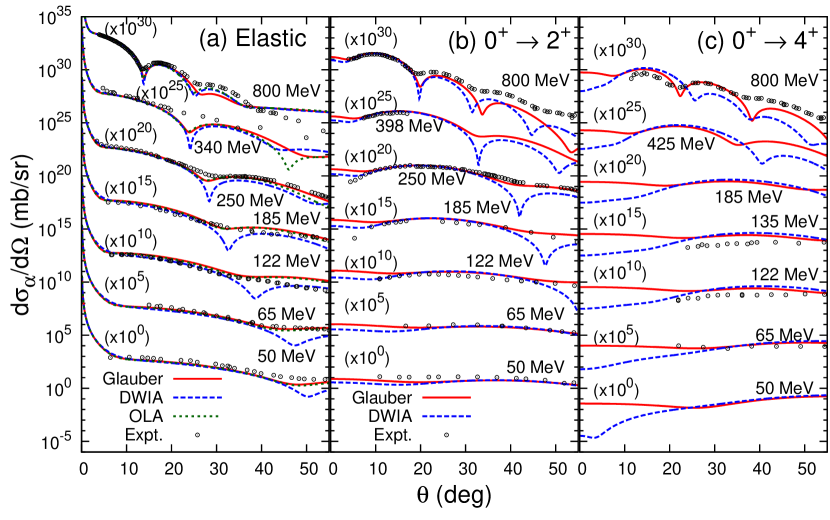
Figure 1: (a) Elastic and (b) inelastic scattering differential cross sections of $0^{+}\to 2^{+}$ and (c) $0^{+}\to 4^{+}$ for proton-¹²C scattering. The results with the optical-limit approximation (OLA) and the eikonal-distorted-wave-impulse approximation (DWIA) are also plotted for comparison. Experimental data are taken from Refs.  [37, 38, 39, 40, 41, 42, 43, 44, 45] for the elastic scattering, Refs. [46, 47, 39, 41, 48, 42, 43, 49, 50] for the $0^{+}\to 2^{+}$ inelastic scattering, and Refs.  [39, 41, 51, 50] for the $0^{+}\to 4^{+}$ inelastic scattering. Experimental error bars are omitted since they are small.

Figure 1 plots the elastic and inelastic differential scattering cross sections of the proton-¹²C system. The Glauber calculations fairly well reproduce the elastic and inelastic scattering cross sections from the ground state to the $2^{+}$ and $4^{+}$ states up to the second cross section minima at incident energy from 50 to 800 MeV. Here we stress that the two parameters of the wave function are determined only from the static structure information, the rms radius and $B(E2)$. No adjustable parameter is introduced in this reaction theory, which strengthens the predictive power.

In order to compare the Glauber calculation with the standard approximated methods, we plot in Fig. 1, the cross sections with the DWIA obtained by Eqs. (13) and (17). For the elastic scattering differential cross sections, the standard OLA results given by Eq. (11) are also plotted. The OLA results are almost identical with the Glauber ones up to the second dip of the elastic scattering differential cross sections. The OLA takes into account most of contributions due to the multiple-scattering processes in the proton-nucleus scattering. We remark a recent interesting application of the OLA in which the surface diffuseness of the nuclear density distribution can be extracted from the proton-nucleus elastic scattering [52]. The standard OLA appears to be more efficient expansion than that done in the DWIA as the DWIA results can only reproduce the elastic scattering cross sections at the forward angle up to the first dip.

The deviation between the Glauber and DWIA calculations becomes more apparent in the inelastic scattering cross sections. Though the DWIA calculations reproduces the cross sections around the peaks, we see large deviation at the forward angles, and at the backward angles with increase in the incident energy. The deviation becomes drastic in the inelastic scattering cross sections to the $4^{+}$ state. This is because the one-step approximation made in the DWIA is not sufficient to describe the whole inelastic processes, whereas the present theory fully takes into account the multiple-scattering or multistep processes within the Glauber theory. We will address this matter in detail later in Sec. 4.

Figure 2 displays the elastic and inelastic scattering differential cross sections of proton-²⁰Ne systems incident at 800 MeV, where the experimental data are available. The theoretical calculations nicely reproduce the experimental cross sections. Though the difference between the Glauber and approximated calculations is not as large as that of the proton-¹²C case in the elastic and $0^{+}\to 2^{+}$ inelastic scattering differential cross sections, we again see non-negligible difference in the $0^{+}\to 4^{+}$ inelastic scattering cross sections.

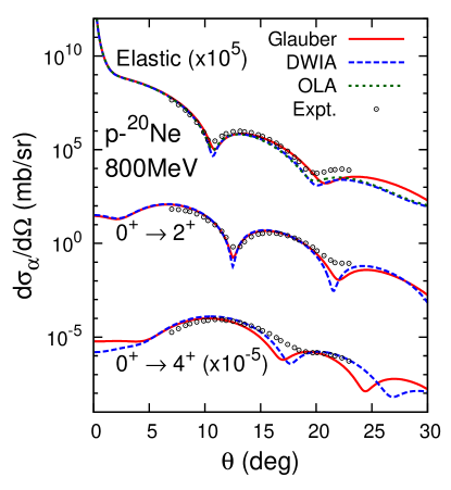
Figure 2: Elastic and inelastic scattering differential cross sections of proton-²⁰Ne scattering at 800 MeV. Experimental data are taken from Ref. [53].

Let us discuss proton-²⁸Si scattering, where we consider both the oblate and prolate deformations which cannot be constrained only by the $B(E2)$ value. Figure 3 compares the elastic and inelastic scattering differential cross sections with the prolate and oblate wave functions of ²⁸Si at incident energy from 50 MeV to 1 GeV. Again, overall agreement between the theory and experimental cross sections is obtained. For the elastic scattering differential cross sections, the calculated cross sections with the oblate and prolate wave functions give almost identical results because the elastic scattering differential cross sections at the forward angles are sensitive to the nuclear radius which is taken as the same for the oblate and prolate wave functions in this study. For the inelastic scattering from the ground to the $2^{+}$ states, we see small differences at the forward angles implying that the cross sections have more information about the quadrupole deformation than that of the $B(E2)$ value. No difference between the cross sections with the oblate and prolate wave functions is found at the scattering angles where the experimental data are available.

A nuclear shape of ²⁸Si has been attracted much interest for a long time [59, 60, 61]. Recent microscopic model calculations showed the oblate and prolate shapes coexist in its spectrum [62, 63, 64]. The difference between the oblate and prolate wave functions can clearly be seen in the inelastic scattering differential cross sections to the $4^{+}$ state. The difference between the cross sections with the oblate and prolate wave functions is significantly large at 155 and 180 MeV allowing one to distinguish the nuclear shape of ²⁸Si. The experimental cross sections are better reproduced by the theoretical cross sections with the oblate wave function. We remark that the recent alpha-nucleus inelastic scattering measurement supports the oblate ground state which is consistent with the Skyrme-Hartree-Fock calculation with the SkM* interaction  [65]. Since the difference becomes more apparent at the higher incident energies, measurement at such high energy will be important as it reveals the nuclear shape of ²⁸Si. We note either the prolate or oblate shape are assumed for ²⁸Si wave function in this work. Use of a more realistic wave function with a mixture of the oblate and prolate shapes are interesting to be worth studying in the future.

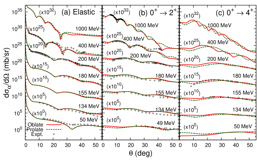
Figure 3: (a) Elastic and (b) inelastic scattering differential cross sections of $0^{+}\to 2^{+}$ and (c) $0^{+}\to 4^{+}$ for proton-²⁸Si scattering. The oblate and prolate wave functions are employed. See text for details. Experimental data are taken from Refs. [54, 55, 56] for the elastic scattering, Refs. [57, 55, 56, 58] for the $0^{+}\to 2^{+}$ inelastic scattering, and Refs. [57, 56] for for the $0^{+}\to 4^{+}$ inelastic scattering.

4 Discussion: Incident energy dependence of the inelastic cross sections

We have confirmed that our theory shows a fairly good description of the inelastic scattering differential cross sections to the $2^{+}$ and $4^{+}$ states for ¹²C, ²⁰Ne, ²⁸Si in a wide range of the incident energies. The magnitude of the inelastic scattering cross section to an angular momentum $J$ state is expected to be proportional to the $B(EJ)$ value. In this section, we discuss which structure information is actually probed by the inelastic cross sections through an analysis of their incident energy dependence.

Figure 4 displays the inelastic scattering cross sections from the ground state to the $2^{+}$ and $4^{+}$ states for ¹²C, ²⁰Ne, and ²⁸Si as a function of the incident energies. The behavior follows the incident-energy dependence of the $pN$ cross sections or the profile functions [18]: The inelastic scattering cross sections for all the nuclei are large at the low incident energies and become smaller with increasing the incident energies and again slightly increases at the higher energy end. We see some difference between the inelastic scattering cross sections to the $2^{+}$ state with the oblate and prolate wave functions of ²⁸Si at the low incident energies despite the fact that the two systems give the same $B(E2)$ value, implying that the proton-nucleus inelastic processes at low-incident energies also contains the information other than that of the $B(E2)$ value but some dynamical properties of the scattering. The inelastic scattering cross sections to the $4^{+}$ state exhibit the same trend and their magnitudes are one order of magnitude smaller than those to the $2^{+}$ state. The cross sections tend to be larger at the low-incident energies where the effective interaction range becomes longer [18] because the rotational excitation takes place at the nuclear surface.

We also plot the results with the DWIA. For the $0^{+}\to 2^{+}$ inelastic scattering, the DWIA calculations work fairly well as the deviation from the Glauber calculations are small at incident energies higher than $\sim$150 MeV, whereas they underestimate the Glauber cross sections at the lower incident energies. For ²⁰Ne, the DWIA calculations reproduce the Glauber calculations even at the low-incident energies except for the lowest cases where they are overestimated. The effects of the multiple-scattering may be small as the ²⁰Ne nucleus is well deformed ($\beta_{2}=0.572$).

For the $0^{+}\to 4^{+}$ inelastic scattering, the DWIA calculations show the similar incident-energy dependence as we observed for the $0^{+}\to 2^{+}$ scattering but for ¹²C case the DWIA underestimate and for ²⁰Ne case it overestimate the Glauber cross sections. For ²⁸Si, the cross sections with the oblate and prolate wave functions show quite different behavior: Despite the fact that the Glauber calculations with the oblate and prolate wave functions give the almost the same cross sections, the DWIA with the prolate wave functions predicts much smaller cross sections than those with the oblate wave functions. This trend may be related to the $B(E4;4^{+}\to 0^{+})$ value of ²⁸Si: 1850 (50.4) $e^{2}$fm⁸ with the oblate (prolate) wave function, and $[B(E4)_{\rm oblate}/B(E4)_{\rm prolate}]^{1/4}\sim 2.5$. Although a direct comparison between the $B(E4)$ value and the $0^{+}\to 4^{+}$ inelastic scattering cross section is not straightforward, a smaller $B(E4)$ value gives a smaller inelastic cross section to the $4^{+}$ state with the DWIA calculation that only takes into account the direct transition from the ground state to the $4^{+}$ state. However, in reality, the $0^{+}\to 4^{+}$ inelastic scattering occurs not only through the direct transition but also through the other multistep transitions leading to the same magnitude of the cross section with the oblate wave function.

The all discussions above become more transparent by calculating the inelastic scattering reaction probability distribution defined by

$$P_{\alpha}(J_{0}\to J_{\alpha};\bm{b})=\frac{1}{2J_{0}+1}\sum_{M_{0},M_{\alpha}}\left|\mathcal{T}_{\alpha}(J_{0}M_{0}\to J_{\alpha}M_{\alpha};\bm{b})\right|^{2},$$ (24)

where $\sigma_{\alpha}=\int d\bm{b}\,P_{\alpha}(J_{0}\to J_{\alpha};\bm{b})$. Figure 5 plots the reaction probability distributions defined by Eq. (24) calculated with the oblate and prolate wave functions of ²⁸Si as a function of impact parameters. The incident energies are chosen as 100, 200, 550, and 1000 MeV. It can be clearly seen that the inelastic reaction mainly occurs at the surface regions. At the lower incident energies, the probabilities show overall enhancement because the proton-nucleon total cross sections become larger and their effective interaction ranges are longer. The probability distributions to the $2^{+}$ state is similar to each other, whereas these to the $4^{+}$ state behave quite differently even their peak positions are different. Recalling that the inelastic scattering differential cross sections are obtained by a Fourier transform of the Glauber transition amplitude $\sim\mathcal{T}_{\alpha}(J_{0}M_{0}\to J_{\alpha}M_{\alpha};\bm{b})$, the oblate and prolate natures of the wave function is imprinted on the inelastic scattering differential cross sections to the $4^{+}$ state as shown in Fig. 3.

We also plot the results with the DWIA. For the $2^{+}$ states, the DWIA works fairly well as we already see in Fig. 4. In case of the $4^{+}$ state, the amplitudes with the DWIA calculations are overestimated (underestimated) than the Glauber calculations for the oblate (prolate) wave functions, respectively, and even their peak positions are different. Since the multiple-scattering effects are significant and mask the direct hexadecapole transition through the inelastic scattering processes, the $0^{+}\to 4^{+}$ inelastic scattering cross sections cannot be a direct observable of $B(E4)$ in this incident energy range.

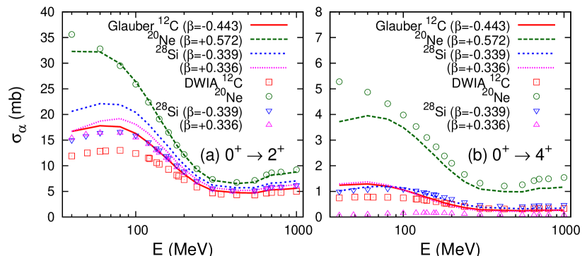
Figure 4: Inelastic scattering cross sections of (a) $0^{+}\to 2^{+}$ and (b) $0^{+}\to 4^{+}$ transitions for proton-¹²C, ²⁰Ne, and ²⁸Si scattering as a function of incident energy.

Figure 5: Reaction probabilities of the inelastic cross sections of (top) $0^{+}\to 2^{+}$ and (bottom) $0^{+}\to 4^{+}$ transitions at incident energies of (a) 100, (b) 200, (c) 550, and (d) 1000 MeV. The vertical thin line indicates the nuclear radius of ²⁸Si, $\sqrt{\frac{5}{3}\left<r^{2}_{p}\right>}=3.89$ fm. See text for details.

5 Application: Interaction cross sections

So far, we have investigated the inelastic scattering cross sections of ¹²C, ²⁰Ne, and ²⁸Si. In this section, as an application of this theory, we evaluate how large these inelastic scattering cross sections in comparison to the total reaction cross section ($\sigma_{R}$). This will be practically useful to compare with the experimentally observed interaction cross sections $(\sigma_{I})$, which can directly be measured by the transmission method as a change of the mass number [66] that involves the inelastic cross sections to the bound excited states (BES). Since one needs to make complicated corrections to obtain $\sigma_{R}$ experimentally, for a practical reason, $\sigma_{I}\simeq\sigma_{R}$ has often been assumed.

Though it may be a good approximation at high incident energy as all collisions lead to the direct breakup to the unbound states, this difference actually affects the precision of the radius extraction. The reliable estimation of the inelastic cross sections is important, e.g., for the precise determination of the neutron-skin thickness using the method proposed in Ref. [67, 22] in which the incident-energy dependence of $\sigma_{R}$ on a proton target is utilized. Though, in this work, the projectile nuclei is limited only to ¹²C, ²⁰Ne, and ²⁸Si, it is useful to know how much contributions of such inelastic processes involved in $\sigma_{R}$.

We quantify the energy dependence of the difference between $\sigma_{I}$ and $\sigma_{R}$. Theoretically $\sigma_{R}$ can easily be calculated by subtracting the survival probability $|\mathcal{T}_{0}(\bm{b})|^{2}$ from unity and integrating it over $\bm{b}$ as

$$\sigma_{R}=\int d\bm{b}\,\left(1-|\mathcal{T}_{0}(\bm{b})|^{2}\right).$$ (25)

To obtain $\sigma_{I}$, one has to make corrections due to the inelastic processes to the BES, which make some complications to the theoretical calculations. $\sigma_{I}$ can be evaluated by subtracting all the inelastic cross sections going to the BES from $\sigma_{R}$ as

$$\sigma_{I}=\sigma_{R}-\sum_{\alpha\in{\rm BES}}\sigma_{\alpha},$$ (26)

where the BES included in the calculations are the $2^{+}$ state for ¹²C; and the $2^{+}$ and $4^{+}$ states for ²⁰Ne and ²⁸Si. We note that ²⁸Si has the other BES which cannot be described by the rotational excitation. Therefore, the $\sigma_{I}$ values for ²⁸Si evaluated in this paper provide their upper limit.

Figure 6 plots the ratio of the interaction cross section to the total reaction cross section, $\sigma_{I}/\sigma_{R}$. As expected, the difference between $\sigma_{I}$ and $\sigma_{R}$ becomes small with increasing the incident energies, which are 2–3% to $\sigma_{R}$. Since the inelastic reaction or rotational excitation mainly occurs in the surface region of the nucleus, the inelastic cross section increases and becomes at most $\sim 5$% contribution to the total reaction cross section at around 100 MeV, where the effective interaction range becomes longer than that at the high incident energy. In the case of ²⁰Ne, where the $B(E2)$ values are largest among the four wave functions, the difference becomes largest at most $\sim 7$%,

One needs to care about those possible uncertainties in the radius extraction using a proton probe. For unstable nuclei, in general, the number of BES is smaller than those of the stable nuclei. Thus, the difference of $\sigma_{I}$ and $\sigma_{R}$ is expected to be less (or zero, if there is no BES) than the cases presented in this paper.

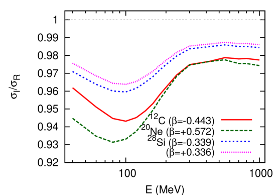
Figure 6: Ratio of the interaction to total reaction cross sections, $\sigma_{I}/\sigma_{R}$, for proton-¹²C, ²⁰Ne, and ²⁸Si scattering as a function of incident energy. Note that only $0^{+}\to 2^{+}$ and $0^{+}\to 4^{+}$ inelastic scattering cross sections are considered for ²⁸Si, giving the upper limit of $\sigma_{I}$. See text for more details.

6 Summary

In order to bridge the nuclear wave function with the direct reaction observables, we have performed a parameter-free reaction calculation for the high-energy proton-nucleus inelastic processes based on the Glauber theory. The multiple-scattering processes within the Glauber theory are fully taken into account by evaluating the Glauber amplitude completely with the help of the factorization technique. Inputs to the theory are the profile function and the wave function of a target (or projectile) nucleus. Once they are set, the theory has no adjustable parameter.

A power of this method has been demonstrated by some examples of the proton inelastic scattering of ¹²C, ²⁰Ne, and ²⁸Si. Their ground- and excited-state wave functions are described by the angular momentum projection of a deformed intrinsic wave function. The axially-symmetric harmonic-oscillator wave function is used as a simplest choice where its size and degree-of-deformation is fixed so as to reproduce the measured charge radius and reduced electric-quadrupole transition probability. Experimental elastic and inelastic scattering differential cross section data are well reproduced without introducing any adjustable parameter. Our results show the higher order terms in the multiple-scattering operator play a significant role in describing such inelastic scattering reactions where the nuclear excitation occurs mainly at the surface region. We find that the inelastic scattering differential cross sections to the $4^{+}$ state of ²⁸Si at the high incident energies are useful observable to study the details of the wave function, i.e., the nuclear shape. We have shown that the multiple-scattering or multistep processes are important in describing the $0^{+}\to 4^{+}$ inelastic scattering cross sections, which is not only through the direct $0^{+}\to 4^{+}$ transition but also through the other multistep transitions. As an application of this theory, we evaluate the contribution of the inelastic processes to the total reaction cross section which can be useful to estimate the uncertainties in the radius extraction from the interaction cross section measurement.

In this paper, we have tested the validity of our method for well-known nuclei using a simple deformed-harmonic-oscillator wave function. The reaction theory developed in this work is rather general formulation as it only requires a multi-Slater determinant wave function. Use of elaborated wave functions is interesting that unveils the structure of unstable nuclei and the role of the excess neutrons (protons) with a systematic measurement of the inelastic scattering cross sections. The extension along this direction is straightforward and will be reported elsewhere.

Appendix A Evaluation of the scattering amplitude

Let us write Eq. (4) in a more calculable form. Since the beam is unpolarized, we can choose any direction for the axis for the quantization. Taking $z$ as the quantization axis, the Glauber amplitude can easily be factorized as

$$\mathcal{T}_{\alpha}(J_{0}M_{0}\to J_{\alpha}M_{\alpha};\bm{b})=\tau_{\alpha}(J_{0}M_{0}\to J_{\alpha}M_{\alpha};b)e^{i(M_{0}-M_{\alpha})\phi}.$$ (27)

With this expression, we can easily carry out the integration over the azimuthal angle $\phi$ by expressing $\bm{b}$ with the polar coordinate $(b,\phi)$. The scattering amplitude (4) can be written more explicitly as

$$f_{\alpha}(q)=i^{|M_{0}-M_{\alpha}|+1}k\int_{0}^{\infty}db\,bJ_{|M_{0}-M_{\alpha}|}(qb)\tau_{\alpha}(J_{0}M_{0}\to J_{\alpha}M_{\alpha};b).$$ (28)

Here the integral expression of the Bessel function of the first kind

$$J_{n}(x)=\frac{1}{2\pi i^{n}}\int_{0}^{2\pi}e^{ix\cos\phi+in\phi}\,d\phi,\qquad(n\geq 0),$$ (29)

is used.

Appendix B Matrix elements with rotated wave functions

As Eq. (10) in Sec. 2.1, the angular momentum projected total wave function is expressed by a superposition of many Slater determinant wave functions. In this Appendix, we give more details about the evaluation of the Glauber amplitude. In this paper, we assume the ground- and excited-state wave functions are generated from the same intrinsic state. The expression of the amplitude with an $A$-body operator $\prod_{j=1}^{A}\mathcal{O}_{j}$ can be written with the rotated single-particle wave functions as

$$\left<\Phi_{\alpha;J_{\alpha}M_{\alpha}}\right|\prod_{j=1}^{A}\mathcal{O}_{j}\left|\Phi_{0;J_{0}M_{0}}\right>$$

$$=\mathcal{N}_{M_{\alpha}0}^{J_{\alpha}}\mathcal{N}_{M_{0}0}^{J_{0}}\iint\,d\omega^{\prime}\,d\omega\,[\mathcal{D}_{M_{\alpha}0}^{J_{\alpha}}(\omega^{\prime})]^{*}\mathcal{D}_{M_{0}0}^{J_{0}}(\omega)\,{\rm det}\left\{\mathcal{M}(\omega^{\prime},\omega)\right\}$$ (30)

with

$$\left\{\mathcal{M}(\omega^{\prime},\omega)\right\}_{jl}=\int d\bm{r}[\phi_{j}(\bm{r}(\omega^{\prime}))]^{*}\mathcal{O}_{j}\phi_{l}(\bm{r}(\omega))\sum_{m^{\prime},m}[\mathcal{D}^{1/2}_{m_{j}m^{\prime}}(\omega^{\prime})]^{*}\mathcal{D}^{1/2}_{m_{l}m}(\omega)\delta_{m_{j},m_{l}},$$ (31)

where $\bm{r}(\omega)=R^{-1}(\omega)\bm{r}$ with the inverse of the rotation matrix $R(\omega)$. Note that the single-particle wave function between the other rotated states is not orthogonal. The matrix element of a one-body operator $\sum_{j=1}^{A}\mathcal{O}_{j}$ can also be evaluated with

$$\left<\Phi_{\alpha;J_{\alpha}M_{\alpha}}\right|\sum_{j=1}^{A}\mathcal{O}_{j}\left|\Phi_{0;J_{0}M_{0}}\right>$$

$$=\mathcal{N}_{M_{\alpha}0}^{J_{\alpha}}\mathcal{N}_{M_{0}0}^{J_{0}}\sum_{j,l=1}^{A}\iint\,d\omega^{\prime}\,d\omega\,[\mathcal{D}_{M_{\alpha}0}^{J_{\alpha}}(\omega^{\prime})]^{*}\mathcal{D}_{M_{0}0}^{J_{0}}(\omega)\,\{\mathcal{M}(\omega^{\prime},\omega)\}_{jl}\,{\rm det}\left\{\tilde{\mathcal{B}}^{(jl)}(\omega^{\prime},\omega)\right\},$$ (32)

where $\tilde{\mathcal{B}}^{(jl)}$ is a cofactor matrix obtained by omitting the $j$th row and the $l$th column from a matrix $\mathcal{B}$ whose elements are defined by

$$\left\{\mathcal{B}(\omega^{\prime},\omega)\right\}_{st}=\int\,d\bm{r}\,[\phi_{s}(\bm{r}(\omega^{\prime}))]^{*}\phi_{t}(\bm{r}(\omega)).$$ (33)

References

- [1] H.J. Ong, N. Imai, D. Suzuki, H. Iwasaki, H. Sakurai et al., Phys. Rev. C 78 (2008) 014308.
- [2] M. Wiedeking, P. Fallon, A.O. Macchiavelli, J. Gibelin, M.S. Basunia, Phys. Rev. Lett. 100 (2008) 152501.
- [3] M. Petri, P. Fallon, A.O. Macchiavelli, S. Paschalis, K. Starosta et al., Phys. Rev. Lett. 107 (2011) 102501.
- [4] P. Voss, T. Baugher, D. Bazin, R. M. Clark, H. L. Crawford, Phys. Rev. C 86 (2012) 011303(R).
- [5] G. Kraus, P. Egelhof, C. Fischer, H. Geissel, A. Himmler et al. Phys. Rev. Lett. 73 (1994) 1773.
- [6] N. Aoi, S. Kanno, S. Takeuchi, H. Suzuki, D. Bazin et al., Phys. Lett. B 692 (2010) 302.
- [7] J. Tanaka, R. Kanungo, M. Alcorta, N. Aoi, H. Bidaman, Phys. Lett. B 774 (2017) 268.
- [8] T. Matsumoto, J. Tanaka, K. Ogata, arXiv: 1711.07209.
- [9] R.J. Glauber, Lectures in Theoretical Physics, edited by W.E. Brittin and L.G. Dunham (Interscience, New York, 1959) Vol. 1, p.315.
- [10] W. Horiuchi, T. Inakura, T. Nakatsukasa, Y. Suzuki, Phys. Rev. C 86 (2012) 024614.
- [11] W. Horiuchi, T. Inakura, T. Nakatsukasa, Y. Suzuki, JPS Conf. Proc. 6 (2015) 030079.
- [12] Y. Ogawa, K. Yabana, Y. Suzuki, Nucl. Phys. A 543 (1992) 722.
- [13] J.S. Al-Khalili, J.A. Tostevin, Phys. Rev. Lett. 76 (1996) 3903.
- [14] J.S. Al-Khalili, J.A. Tostevin, I.J. Thompson, Phys. Rev. C 54 (1996) 1843.
- [15] T. Nagahisa, W. Horiuchi, Phys. Rev. C 97 (2018) 054614.
- [16] Y. Abgrall, J. Labarsouque, B. Morand, Nucl. Phys. A 271 (1976) 477.
- [17] L. Ray, Phys. Rev. C 20 (1979) 1857.
- [18] B. Abu-Ibrahim, W. Horiuchi, A. Kohama, Y. Suzuki, Phys. Rev. C 77 (2008) 034607; ibid 80 (2009) 029903; 81 (2010) 019901.
- [19] B. Abu-Ibrahim, S. Iwasaki, W. Horiuchi, A. Kohama, Y. Suzuki, J. Phys. Soc. Jpn., Vol. 78 (2009) 044201.
- [20] W. Horiuchi, Y. Suzuki, P. Capel, and D. Baye, Phys. Rev. C 81 (2010) 024506.
- [21] Y. Suzuki, W. Horiuchi, S. Terashima, R. Kanungo, F. Ameil et al., Phys. Rev. C 94 (2016) 011602(R).
- [22] W. Horiuchi, S. Hatakeyama, S. Ebata, Y. Suzuki, Phys. Rev. C 93 (2016) 044611.
- [23] Y. Suzuki, R.G. Lovas, K. Yabana, K. Varga, Structure and reactions of light exotic nuclei (Taylor & Francis, London, 2003).
- [24] K. Varga, S.C. Pieper, Y. Suzuki, R.B. Wiringa, Phys. Rev. C 66 (2002) 034611.
- [25] N. Metropolis, A. Rosenbluth, M. Rosenbluth, E. Teller, J. Chem. Phys. 21 (1953) 1087.
- [26] R.H. Bassel, C. Wilkin, Phys. Rev. 174 (1968) 1179.
- [27] S. Hatakeyama, S. Ebata, W. Horiuchi, M. Kimura, J. Phys.: Conf. Ser. 569 (2014) 012050.
- [28] S. Hatakeyama, S. Ebata, W. Horiuchi, M. Kimura, JPS Conf. Proc., Vol. 6 (2015) 030096.
- [29] Y. Kanada-En’yo, M. Kimura, A. Ono, Prog. Theor. Exp. Phys. 2012 (2012) 01A202, and references therein.
- [30] H. Feldmeier, Nucl. Phys. A 515 (1990) 147.
- [31] H. Feldmeier, K. Bieler, J. Schnack, Nucl. Phys. A 586 (1995) 493.
- [32] J. Saudinos, C. Wilkin, Ann. Rev. Nucl. Sci. 24 (1974) 341.
- [33] Y. Alexander, A. S. Rinat (Reiner), Ann. of Phys. 82 (1974) 301.
- [34] Y. Abgrall, B. Morand, E. Caurier, Nucl. Phys. A 192 (1972) 372.
- [35] I. Angeli, K.P. Marinova, At. Data. Nucl. Data Tables 99 (2013) 69.
- [36] B. Priytychenko, M. Birch, B. Singh, M. Horoi, At. Data Nucl. Data Tab. 107 (2016) 1.
- [37] A.A. Rush, E.J. Burge, D.A. Smith, Nucl. Phys. A 166 (1971) 378.
- [38] M. Ieiri, H. Sakaguchi, M. Nakamura, H. Sakamoto, H. Ogawa et al., Nucl. Inst. Meth. Phys. Res. A 257 (1987) 253.
- [39] S. Kato, K. Okada, M. Kondo, K. Hosono, T. Saito et al., Phys. Rev. C 31 (1985) 1616.
- [40] H.O. Meyer, P. Schwandt, W.W. Jacobs, J.R. Hall, Phys. Rev. C 27 (1983) 459.
- [41] J.R. Comfort, Sam M. Austin, P.T. Debevec, G.L. Moake, R.W. Finlay et al, Phys. Rev. C 21 (1980) 2147.
- [42] A. Ingemarsson, O. Jonsson, A. Hallgren, Nucl. Phys. A 319 (1979) 377.
- [43] H. O. Meyer, P. Schwandt, R. Abegg, C.A. Miller, K. P. Jackson et al., Phys. Rev. C 37 (1988) 544.
- [44] R.E. Richardson, W.P. Ball, C.E. Leith, Jr., B.J. Moyer, Phys. Rev. 86 (1952) 29.
- [45] G.S. Blanpied, G.W. Hoffmann, M.L. Barlett, J.A. McGill, S.J. Greene et al., Phys. Rev. C 23 (1981) 2599.
- [46] J.A. Fannon, E.J. Burge, D.A. Smith, N.K. Ganguly, Nucl. Phys. A 97 (1967) 263.
- [47] N.M. Clarke, E.J. Burge, D.A. Smith, J.C. Dore, Nucl. Phys. A 157 (1970) 145.
- [48] M. Hugi, W. Bauhoff, H.O. Meyer, Phys. Rev. C 28 (1983) 1.
- [49] K.W. Jones, C. Glashausser, R. de Swiniarski, F.T. Baker, T.A. Carey et al. Phys. Rev. C 50 (1994) 1982.
- [50] G.S. Blanpied, W.R. Coker, R.P. Liljestrand, G.W. Hoffmann, L. Ray et al., Phys. Rev. C 18 (1978) 1436.
- [51] W. Bauhoff, S.F. Collins, R.S. Henderson, G.G. Shute, B.M. Spicer et al., Nucl. Phys. A 410 (1983) 180.
- [52] S. Hatakeyama, W. Horiuchi, A. Kohama, Phys. Rev. C 97 (2018) 054607.
- [53] G.S. Blanpied, B.G. Ritchie, M.L. Barlett, R.W. Fergerson, G.W. Hoffmann et al., Phys. Rev. C 38 (1988) 2180.
- [54] M. Nakamura, H. Sakaguchi, H. Sakamoto, H. Ogawa, O. Cynshi et al., Nucl. Inst. and Meth. Phys. Res. 212 (1983) 173.
- [55] K. H. Hicks, R. G. Jeppesen, C. C. K. Lin, R. Abegg, K. P. Jackson et al., Phys. Rev. C 38 (1988) 229.
- [56] Q. Chen, J.J. Kelly, P.P. Singh, M.C. Radhakrishna, W.P. Jones et al., Phys. Rev. C 41 (1990) 2514.
- [57] K. Amos, W. Bauhoff, Nucl. Phys. A 424 (1984) 60.
- [58] G.D. Alkhazov et al., Yad. Fiz. 22 (1975) 902.
- [59] A.L. Goodman, G.L. Struble, J. Bar-Touv, A. Goswami, Phys. Rev. C 2 (1970) 380.
- [60] G. Leander, S.E. Larsson, Nucl. Phys. A 239 (1975) 93.
- [61] W. Bauhoff, H. Schultheis, R. Schultheis, Phys. Rev. C 26 (1982) 1725.
- [62] Y. Kanada-En’yo, Phys. Rev. C 71 (2005) 014303.
- [63] T. Ichikawa, N. Itagaki, Y. Kanada-En’yo, Tz. Kokalova, W. von Oertzen, Phys. Rev. C 86 (2012) 031303(R).
- [64] Y. Chiba, Y. Taniguchi, M. Kimura, Phys. Rev. C 95 (2017) 044328.
- [65] T. Peach, U. Garg, Y.K. Gupta, J. Hoffman, J.T. Matta et al., Phys. Rev. C 93 (2016) 064325.
- [66] I. Tanihata, H. Hamagaki, O. Hashimoto, Y. Shida, N. Yoshikawa et al., Phys. Rev. Lett. 55 (1985) 2676.
- [67] W. Horiuchi, Y. Suzuki, T. Inakura, Phys. Rev. C 89 (2014) 011601(R).