All-electron fully relativistic Kohn–Sham theory for solids
based on the Dirac–Coulomb Hamiltonian and Gaussian-type functions

Abstract

We present the first full-potential method that solves the fully relativistic four-component Dirac–Kohn–Sham equation for materials in the solid state within the framework of atom-centered Gaussian-type orbitals (GTOs). Our GTO-based method treats one-, two-, and three-dimensional periodic systems on an equal footing, and allows for a seamless transition to the methodology commonly used in studies of molecules with heavy elements. The scalar relativistic effects as well as the spin–orbit interaction are handled variationally. The full description of the electron–nuclear potential in the core region of heavy nuclei is straightforward due to the local nature of the GTOs and does not pose any computational difficulties. We show how the time-reversal symmetry and a quaternion algebra-based formalism can be exploited to significantly reduce the increased methodological complexity and computational cost associated with multiple wave-function components coupled by the spin–orbit interaction. We provide a detailed description of how to employ the matrix form of the multipole expansion and an iterative renormalization procedure to evaluate the conditionally convergent infinite lattice sums arising in studies of periodic systems. Next, we investigate the problem of inverse variational collapse that arises if the Dirac operator containing a repulsive periodic potential is expressed in a basis that includes diffuse functions, and suggest a possible solution. Finally, we demonstrate the validity of the method on three-dimensional silver halide (Ag$X$) crystals with large relativistic effects, and two-dimensional honeycomb structures (silicene and germanene) exhibiting the spin–orbit-driven quantum spin Hall effect. Our results are well-converged with respect to the basis set limit using standard bases developed for molecular calculations, and indicate that the common rule of removing basis functions with small exponents should not be applied when transferring the molecular basis to solids.

I Introduction

Relativistic effects on band structures and properties of solids containing heavy elements have for a long time been known to have a significant impact on both core and valence electrons Christensen and Seraphin (1971). The effects of relativity on the spectroscopic properties of electrons close to the nuclei (x-ray spectroscopy) were studied as early as in 1933 Pincherle (1933). In contrast, the importance of relativistic effects on valence states located close to the Fermi level was not apparent until 1957 Mayers (1957) when Mayers observed a large relativistic contraction of the 6$s$ orbital and a corresponding expansion of the 5$d$ orbitals in heavy elements such as mercury. Such changes in the size of the atomic orbitals due to relativity can lead to dramatic changes in the structural and physical properties of solids Christensen et al. (1986); Söhnel et al. (2001); Pyykko (1988). For instance, Christensen, Satpathy, and Pawlowska demonstrated that these relativistic effects are responsible for the stable phase of lead being the face-centered cubic (fcc) crystal structure, in contrast to the diamond-like structure adopted by other group 14 elements (C, Si, Ge and Sn) Christensen et al. (1986). It has also been shown that relativistic effects need to be included in theoretical models of solids in order to explains why the ground state of CsAu is insulating and not metallic Christensen and Kollar (1983). Relativity has also been shown to significantly increase the voltage of the lead-acid-battery reaction used in car batteries by 1.7-1.8 V out of the total 2.13 V Ahuja et al. (2011), and lead to a decrease in the melting temperature of mercury by 105 K Calvo et al. (2013), making mercury the only metal that is liquid at room temperature.

A protruding manifestation of relativity in quantum mechanics – the spin–orbit coupling (SOC) – leads to a splitting of bands in materials lacking space inversion symmetry Dresselhaus (1955); Broido and Sham (1985); Rashba and Sherman (1988). These splittings can be remarkably large in transition-metal dichalcogenides Zhu et al. (2011); Heine (2014); Rasmussen and Thygesen (2015); Xu et al. (2014), and are then often referred to as “giant SOC”. SOC plays a paramount role in the field of spintronics Rashba (2000); Wolf et al. (2001); Žutić et al. (2004), topological insulators Kane and Mele (2005); Hasan and Kane (2010), and related spin-Hall effects Sinova et al. (2004, 2015); Kou et al. (2017). SOC has also been shown to open the band gap in two-dimensional honeycomb systems Gmitra et al. (2009); Liu et al. (2011); Xu et al. (2013); Han et al. (2014) and change the stable phase of flerovium (Fl, element 114) from fcc to a hexagonal close packed (hcp) structure Hermann et al. (2010).

Materials exhibiting some of the unique properties mentioned above are rare Bradlyn et al. (2017), however, and the search for novel materials must be aided by first-principles calculations Bansil et al. (2016). Modeling spin–orbit-coupled solid-state systems is far from straightforward, and Kohn–Sham (KS) density functional theory (DFT) Hohenberg and Kohn (1964); Kohn and Sham (1965) is today the only affordable first-principles method at the fully relativistic level of theory with variationally included SOC. For such studies, DFT offers a very favorable compromise between accuracy and computational feasibility. However, we note the promising recent works of Sakuma et al. Sakuma et al. (2011) and Scherpelz et al. Scherpelz et al. (2016) at the GW level of theory.

A critical choice in the modeling of solids is the representation of the one-particle basis functions. There are two major families of basis sets: local functions (e.g. atom-centered orbitals) and plane waves. Plane waves are ill-suited to capture rapid oscillations of wave functions in regions close to the nuclei, and are for this reason often combined with pseudopotentials Vanderbilt (1990). For heavier elements, these pseudopotentials can be constructed from relativistic all-electron calculations Troullier and Martins (1991); Hangele et al. (2012). The use of pseudopotentials sacrifices the possibility to model the nodal structure of the wave functions close to the nuclei and introduces uncontrollable transferability errors. This makes all-electron methods in some cases the preferred method, e.g. for calculations of nuclear magnetic resonance (NMR) shifts Kim et al. (2010).

Relativistic all-electron calculations are possible using the relativistic Korringa–Kohn–Rostoker (KKR) method Takada (1966); Strange et al. (1984); Wang et al. (1992); Der Kellen and Freeman (1996) or by extending Slater’s augmented plane-wave (APW) method Slater (1937) to the Dirac Hamiltonian Loucks (1965); Mattheiss (1966). The APW method divides space into spheres centered at atoms and an interstitial region, and requires solving a secular energy-dependent equation for each band to match KS orbitals at boundaries of the spheres. This approach results in equations with a nonlinear dependence on energies. The method is very accurate, but computationally expensive. To mitigate the computational cost, the APW method can be linearized Andersen (1975); Sjöstedt et al. (2000), leading to the linear-APW (LAPW) and linear muffin-tin orbitals (LMTO) methods, enabling the use of a full potential for all electrons. The LMTO approach has been extended to the relativistic domain Christensen (1978); Godreche (1982); Ebert (1988); Ebert et al. (1988). A relativistic extension of LAPW was first developed by MacDonald, Picket and Koelling MacDonald et al. (1980) and later by Wimmer et al. Wimmer et al. (1981). MacDonald et al. included SOC by a two-step variational method, the so-called second-variational approach, i.e. as a post processing to the spin-non-polarized scalar-relativistic self-consistent procedure. This process is performed on a smaller set of scalar-relativistic eigenfunctions, thus reducing the computational effort considerably. The second-variational approach was later extended and implemented in some of the modern program packages Schwarz et al. (2002); Blaha et al. (2001); Kurz et al. (2004), where the second-variational inclusion of SOC can be employed both self-consistently as well as non-self-consistently.

Both the full-potential LMTO and LAPW methods suffer from limitations when treating systems with deep-lying valence and extended core states Blaha et al. (1992). If SOC is included, severe convergence problems can be encountered Nordström et al. (2000). These limitations are due to the insufficient flexibility of the finite scalar-relativistic basis set for describing Dirac $p_{1/2}$ states in the core region MacDonald et al. (1980); Nordström et al. (2000). Convergence is achieved when the basis is augmented by Dirac $p_{1/2}$ local orbitals in the second variational step Kuneš et al. (2001); Carrier and Wei (2004); Huhn and Blum (2017). Huhn and Blum carried out a benchmark study and a comparison of various LAPW strategies for the evaluation of the SOC contribution Huhn and Blum (2017).

More recently, the linearized methods were generalized by Blöchl to include the pseudopotential approximation, establishing the projector augmented wave (PAW) technique Blöchl (1994); Kresse and Joubert (1999). PAW introduces pseudopotentials as a well-defined approximation, and hence brings transferability errors under control, enabling all-electron calculations of properties in a pseudopotential framework. However, the complexity of the PAW approach makes its extension to e.g. include hybrid density functionals and the study of response properties difficult. A fully relativistic PAW method for both Dirac-type (four-component) and Pauli-type (two-component) equations was formulated by Dal Corso Dal Corso (2010).

An alternate strategy to the use of plane waves, is to expand the KS orbitals in a set of local functions. Such full-potential methods employing numerical orbitals have been extended to include scalar relativistic corrections Suzuki and Nakao (2000); Blum et al. (2009), as well as four-component (4c) SOC Suzuki and Nakao (1999); Koepernik and Eschrig (1999); Opahle (2001); Eschrig et al. (2004). Alternatively, basis functions can be constructed by placing analytic Slater-type orbitals (STOs) or Gaussian-type orbitals (GTOs) on atomic centers. two-component (2c) techniques using STOs were implemented by Philipsen et al. Philipsen et al. (1997); Philipsen and Baerends (2000) and Zhao et al. Zhao et al. (2016) Relativistic calculations on solids with GTOs were reported with scalar-relativistic corrections Geipel and He$\beta$ (1997); Peralta et al. (2005), as well as approximate 2c schemes solving Pauli-type equations Wang and Callaway (1974); Mainkar et al. (1996), or approaches based on the Douglass–Kroll–Hess Hamiltonian Jones et al. (2000); Boettger (2000). While calculations that include scalar-relativistic corrections on solids are common Suzuki and Nakao (2000); Blum et al. (2009); Geipel and He$\beta$ (1997); Peralta et al. (2005), extending nonrelativistic implementations by SOC poses severe methodological challenges due to the appearance of multicomponent spinor structure of the wave functions as well as the need to use complex algebra.

Here, we present the first fully relativistic all-electron full-potential GTO-based method directly solving the 4c Dirac–Kohn–Sham (DKS) equation for periodic systems while treating both the scalar relativistic effects and SOC variationally during the self-consistent optimization procedure. Thus, the approach enables studies of relativistic effects in solids containing elements from the entire periodic table in a consistent manner without the use of the pseudopotential approximation. The variational treatment of SOC is mandatory in studies of materials containing heavy elements, where SOC splittings are of the same magnitude as the effects of the crystal potential, and for which the evaluation of perturbational or non-self-consistent SOC can be insufficient Soven (1965); Sakuma et al. (2011); Huhn and Blum (2017). We will demonstrate that GTOs are a convenient and computationally efficient approach for full-potential relativistic calculations. The local nature of the GTOs makes them amendable to highly efficient linear scaling techniques, as GTOs better reflect the decay properties of operators and density matrices Goedecker (1999). In addition, because periodicity is embedded explicitly in the local basis, systems that are periodic in one or two dimensions (polymers and slabs) can be studied using atom-centered GTOs while avoiding the requirement to repeat the polymer or slab in the non-periodic dimensions Miró et al. (2014). This eliminates the concern in calculations on such systems using plane waves that there will be spurious self interactions between the system studied and its periodic images. In contrast to LMTO and LAPW, GTOs can treat both core and valence electrons on an equal footing, the quality being independent of a fixed linearization energy. Furthermore, here we will demonstrate that a systematic convergence to the basis limit is possible with GTOs, and discuss specific problems arising in the nonrelativistic and 4c cases if the diffuse functions are included in a local basis.

The presented 4c method builds on a transparent and efficient quaternion algebra-based formulation of time-reversal-symmetric operators in real and reciprocal space employing a Kramers-restricted kinetically balanced basis. We implemented this method into the 4c ReSpect program package res , and utilized integral screening techniques based on quaternion algebra Konecny et al. (2018); Repisky et al. . The implementation exploits the full $\bm{k}$-point sampling of the first Brillouin zone, and allows to use irreducible unit cells for all lattice structures. Our approach builds on previous nonrelativistic methodologies for handling periodic systems with GTOs. This includes the pioneering works of Pisani, Dovesi and coworkers Pisani and Dovesi (1980); Dovesi et al. (1983), and the more recent implementations of Towler, Zupan and Causá Towler et al. (1996) and of Łazarski, Burow and Sierka Łazarski et al. (2015).

The rest of the paper is organized as follows. In Sec. II, we establish the main principles of our 4c GTO-based method for the solid state. In Sec. II.1, we concentrate on the general formulation of the working equations, in Sec. II.2, we define the 4c density and the density matrix in real-space GTOs, Sec. II.3 shows consequences of the time-reversal symmetry on the structure of operators in both real space and reciprocal space, and these concepts are further developed in Sec. II.4 in a quaternion formulation. In Sec. II.5, we derive how the Coulomb potential and energy are evaluated using the 4c real-space GTOs, before we in Sec. II.6 analyze the problem of the long-range electrostatic lattice sums, and describe its solutions within our theoretical framework. In Sec. II.7, we derive the exchange–correlation contributions. Practical implementation details and approximations required in realistic calculations are described in Sec. III. In Sec. IV.1, we discuss problems emerging in the nonrelativistic solid-state calculations associated with diffuse functions in local basis sets, and in Sec. IV.2, we outline a new complication that arises in our relativistic method if we include diffuse functions in the basis. Results for the silver halide crystals and 2D hexagonal structures are shown and discussed in Sec. V, before we in Sec. VI give some concluding remarks and an outlook.

II Theory

II.1 General framework

In this section, we outline the basic GTO-based scheme we use to solve the 4c DKS equations for periodic systems. Unless otherwise stated, we employ atomic units, setting the elementary charge $e$, the electron rest mass $m_{e}$ and reduced Planck’s constant $\hbar$ to unity. Throughout this paper, Einsteins’s implicit summation over repeated indices is assumed.

The fundamental building units of the presented theory are the scalar atom-centered normalized primitive Cartesian GTOs Boys (1950); Obara and Saika (1986)

$$g_{\mu}(\bm{r})\equiv\mathcal{N}(x-A_{x})^{l_{x}}(y-A_{y})^{l_{y}}(z-A_{z})^{l_{z}}e^{-\alpha(\bm{r}-\bm{A})^{2}},$$ (1)

where $\mathcal{N}$ is the normalization constant, $\alpha$ is the Gaussian exponent, $\bm{l}\equiv(l_{x},l_{y},l_{z})$ are the Cartesian angular momenta, and $\bm{A}$ and $\bm{r}$ are the nuclear and electron coordinates, respectively. Basis representations of the solutions to the DKS equations are constructed in three steps. First, 4c basis bispinors $\chi_{\mu}$ for a reference unit cell are formed

$$\chi_{\mu}(\bm{r})\equiv\begin{pmatrix}\chi^{L}_{\mu}(\bm{r})&0_{2}\\ 0_{2}&\chi^{S}_{\mu}(\bm{r})\end{pmatrix},$$ (2)

using 2c spinors $\chi^{L}_{\mu}$ and $\chi^{S}_{\mu}$ defined for the so-called large ($L$) and small ($S$) components, respectively, as

$$\chi^{L}_{\mu}(\bm{r}) \equiv\mathbb{I}_{2}\otimes g_{\mu}(\bm{r}),$$ (3a)

$$\chi^{S}_{\mu}(\bm{r}) \equiv\frac{1}{2c}(\bm{\sigma}\cdot\bm{p})g_{\mu}(\bm{r}),$$ (3b)

where $\mathbb{I}_{2}$ is the $2\times 2$ identity matrix, $\bm{\sigma}$ are the Pauli matrices, $\bm{p}\equiv-i\bm{\nabla}$ is the electron momentum operator, and $c$ is the speed of light. The construction of the small-component basis in Eq. (3b) utilizes the restricted kinetically balanced (RKB) condition which is essential to achieve variationally stable 4c solutions in a finite basis Stanton and Havriliak (1984). Second, the basis for periodic systems is obtained by translating $\chi_{\mu}$ from the reference unit cell to the unit cell $\bm{m}$ as

$$\chi_{\mu\bm{m}}(\bm{r})\equiv\chi_{\mu}(\bm{r}-\bm{m}),$$ (4)

where the unit cell position vector $\bm{m}$ is

$$\bm{m}=m^{i}\bm{a}_{i},\hskip 22.76219ptm^{i}\in\mathbb{Z},i=1,\ldots,d.$$ (5)

Here, $\mathbb{Z}$ denotes the field of integers, $d$ is the number of periodic dimensions, and $\bm{a}_{i}$ are the primitive vectors that constitute a Bravais lattice. Since all unit cells are equivalent, we choose the central unit cell $\bm{m}=\bm{0}$ to be the fixed reference unit cell. Third, symmetry-adapted Bloch functions for each $\bm{k}$ point from the first Brillouin zone $\mathcal{K}$ are constructed from the real-space GTOs as the Fourier series

$$\varphi_{\mu}(\bm{k};\bm{r})=\frac{1}{\sqrt{|\mathcal{K}|}}\sum_{\bm{m}}e^{i\bm{k}\cdot{\bm{m}}}\chi_{\mu\bm{m}}(\bm{r}),$$ (6)

where the infinite lattice sum is over the whole Bravais lattice. $|\mathcal{K}|$ is the volume of the primitive reciprocal unit cell (first Brillouin zone), and enters the normalization constant to ensure an approximate normalization of the Bloch functions. The symmetry-adapted functions in Eq. (6) satisfy the Bloch condition

$$\varphi_{\mu}(\bm{k};\bm{r}+\bm{m})=e^{i\bm{k}\cdot{\bm{m}}}\varphi_{\mu}(\bm{k};\bm{r}),$$ (7)

by construction, and $\varphi_{\mu}(\bm{k};\bm{r})$ can thus be used as basis functions that block-diagonalize a translationally invariant Hamiltonian.

Our aim is to solve the 4c DKS equations

$$\hat{F}\psi_{p}(\bm{k};\bm{r})=\varepsilon_{p}(\bm{k})\psi_{p}(\bm{k};\bm{r}),$$ (8)

for each band $p$. Here $\varepsilon_{p}(\bm{k})$ and $\psi_{p}(\bm{k};\bm{r})$ are the energy and the crystalline orbital (CO) of the $p$-th band, respectively, and $\hat{F}$ is the 4c Fock operator

$$\hat{F}=\begin{pmatrix}V(\bm{r})&c\bm{\sigma}\cdot\bm{p}\\ c\bm{\sigma}\cdot\bm{p}&V(\bm{r})-2c^{2}\end{pmatrix},$$ (9)

consisting of the one-electron Dirac Hamiltonian Dirac (1928) and the potential $V(\bm{r})$, which in the context of KS DFT contains the mean-field Coulomb potential and the exchange–correlation potential Kutzelnigg (1984); Saue and Helgaker (2002); Komorovsky et al. (2008). Such an approach approximates the two-electron interaction with an instantaneous Coulomb operator, neglecting the relativistic corrections to the electron–electron interaction. We expand the solutions $\psi_{p}(\bm{k};\bm{r})$ of Eq. (8) in terms of the Bloch functions in Eq. (6):

$$\psi_{p}(\bm{k};\bm{r})=\varphi_{\mu}(\bm{k};\bm{r})c^{\mu}_{\phantom{a}p}\,(\bm{k}),$$ (10)

where $c^{\mu}_{\phantom{a}p}(\bm{k})$ are the 4c CO expansion coefficients. Inserting the expansions in Eqs. (10) and (6) into Eq. (8), multiplying the equation with $\varphi^{\dagger}_{\mu^{\prime}}(\bm{k};\bm{r})$ from the left and integrating over spatial coordinates $\bm{r}$, yields the matrix form of the DKS equation in reciprocal space

$$F(\bm{k})c(\bm{k})=S(\bm{k})c(\bm{k})\varepsilon(\bm{k}),$$ (11)

where $\varepsilon(\bm{k})$ is the diagonal matrix of the band energies. $F(\bm{k})$ and $S(\bm{k})$ are reciprocal-space forms of the Fock and overlap matrices, respectively (see Appendix A):

$$F_{\mu\mu^{\prime}}(\bm{k}) =\sum_{\bm{m}}e^{i\bm{k}\cdot{\bm{m}}}F_{\mu\bm{0},\mu^{\prime}\bm{m}},$$ (12a)

$$S_{\mu\mu^{\prime}}(\bm{k}) =\sum_{\bm{m}}e^{i\bm{k}\cdot{\bm{m}}}S_{\mu\bm{0},\mu^{\prime}\bm{m}},$$ (12b)

and

$$F_{\mu\bm{0},\mu^{\prime}\bm{m}} =\int_{\mathbb{R}^{3}}\chi^{\dagger}_{\mu\bm{0}}(\bm{r})\hat{F}\chi_{\mu^{\prime}\bm{m}}(\bm{r})d^{3}\bm{r},$$ (13a)

$$S_{\mu\bm{0},\mu^{\prime}\bm{m}} =\int_{\mathbb{R}^{3}}\chi^{\dagger}_{\mu\bm{0}}(\bm{r})\chi_{\mu^{\prime}\bm{m}}(\bm{r})d^{3}\bm{r}.$$ (13b)

We have here exploited the translational invariance of the Fock operator, which allows us to consider only the reference unit cell $\bm{m}=\bm{0}$ for the bra function $\chi^{\dagger}_{\mu\bm{0}}$, and to solve Eq. (11) independently for each $\bm{k}$. Finally, we express the real-space integrals in Eqs. (13) utilizing Eqs. (2) and (3) to obtain the 4c matrix forms for $F_{\mu\bm{0},\mu^{\prime}\bm{m}}$ and $S_{\mu\bm{0},\mu^{\prime}\bm{m}}$:

$$F_{\mu\bm{0},\mu^{\prime}\bm{m}} =\begin{pmatrix}\mathcal{V}^{LL}&\mathcal{T}\\ \mathcal{T}&\frac{1}{4c^{2}}\mathcal{V}^{SS}-\mathcal{T}\end{pmatrix}_{\mu\bm{0},\mu^{\prime}\bm{m}},$$ (14)

$$S_{\mu\bm{0},\mu^{\prime}\bm{m}} =\begin{pmatrix}\mathcal{S}&0_{2}\\ 0_{2}&\frac{1}{2c^{2}}\mathcal{T}\end{pmatrix}_{\mu\bm{0},\mu^{\prime}\bm{m}},$$ (15)

where the indices $\mu\bm{0},\mu^{\prime}\bm{m}$ are applied to each element of the matrices individually and

$$\mathcal{S}_{\mu\bm{0},\mu^{\prime}\bm{m}} =\mathbb{I}_{2}\otimes\int_{\mathbb{R}^{3}}g_{\mu\bm{0}}(\bm{r})g_{\mu^{\prime}\bm{m}}(\bm{r})d^{3}\bm{r},$$ (16a)

$$\mathcal{T}_{\mu\bm{0},\mu^{\prime}\bm{m}} =\mathbb{I}_{2}\otimes\int_{\mathbb{R}^{3}}g_{\mu\bm{0}}(\bm{r})\frac{p^{2}}{2}g_{\mu^{\prime}\bm{m}}(\bm{r})d^{3}\bm{r},$$ (16b)

$$\mathcal{V}^{LL}_{\mu\bm{0},\mu^{\prime}\bm{m}} =\mathbb{I}_{2}\otimes\int_{\mathbb{R}^{3}}g_{\mu\bm{0}}(\bm{r})V(\bm{r})g_{\mu^{\prime}\bm{m}}(\bm{r})d^{3}\bm{r},$$ (16c)

$$\mathcal{V}^{SS}_{\mu\bm{0},\mu^{\prime}\bm{m}} =\int_{\mathbb{R}^{3}}\left[(\bm{\sigma}\cdot\bm{p})g_{\mu\bm{0}}(\bm{r})\right]^{\dagger}V(\bm{r})\left[(\bm{\sigma}\cdot\bm{p})g_{\mu^{\prime}\bm{m}}(\bm{r})\right]d^{3}\bm{r}.$$ (16d)

Integrals over the GTOs in Eqs. (16) are evaluated analytically using the recurrence scheme of Obara and Saika Obara and Saika (1986); int . If we now let

$$T =\begin{pmatrix}0_{2}&\mathcal{T}\\ \mathcal{T}&-\mathcal{T}\end{pmatrix}, V =\begin{pmatrix}\mathcal{V}^{LL}&0_{2}\\ 0_{2}&\frac{1}{4c^{2}}\mathcal{V}^{SS}\end{pmatrix},$$ (17)

be the 4c kinetic energy matrix and the potential matrix, respectively, where we have omitted the $\mu\bm{0},\mu^{\prime}\bm{m}$ indices, the DKS Fock matrix in Eq. (14) can be partitioned as:

$$F=T+V=T+J+V^{\text{XC}}.$$ (18)

Here, $J$ is the Coulomb and $V^{\text{XC}}$ the exchange–correlation contribution to the potential matrix $V$ (the evaluation of these contributions will be discussed in more detail in Secs. II.5 and II.7, respectively). The Coulomb matrix $J$ contains both the electron-nuclear interaction and the Hartree mean-field interaction term. The exact exchange matrix required for Hartree–Fock theory or hybrid DFT is omitted in this work.

Within the framework of DFT, Eq. (11) must be solved self-consistently, since $V$ contains the mean-field potential as well as the exchange–correlation potential, both of which depend on the electron density and its gradients and which are constructed from the COs $\psi_{i}(\bm{k};\bm{r})$. Eq. (11) is solved in an iterative manner: its solutions are used to build a new Fock matrix $F$, Eq. (11) is then solved for this updated potential until convergence is reached.

II.2 Density and density matrix

In this section, we formulate the real-space 4c reduced one-electron density matrix $D^{\mu\bm{m},\mu^{\prime}\bm{0}}$ and the electron density $\rho_{\text{e}}$ for periodic systems that are used in practice for the construction of the Fock matrix [Eq. (14)] instead of $\psi_{i}(\bm{k};\bm{r})$.

The reciprocal-space density matrix expressed in terms of COs is a diagonal matrix, where the diagonal elements form an occupation vector $f_{p}(\bm{k})$ for each band $p$. $f_{p}(\bm{k})$ is a zero-temperature limit of the Fermi–Dirac distribution

$$f_{p}(\bm{k})=\frac{1}{e^{\beta\left(\varepsilon_{p}(\bm{k})-\mu\right)}+1}\overset{\beta\rightarrow\infty}{\longrightarrow}\vartheta\left(\mu-\varepsilon_{p}(\bm{k})\right),$$ (19)

where $\mu$ is the Fermi level chemical potential, $\beta$ is the inverse temperature, and $\vartheta$ is the Heaviside step function. Bands corresponding to positronic (negative-energy) states are left vacant (see Sec. IV.2). If we let $f(\bm{k})$ denote the diagonal matrix of occupation numbers, we can write the $\bm{k}$-space density matrix in its block-diagonal form as

$$D(\bm{k},\bm{k}^{\prime}) =\delta(\bm{k}-\bm{k}^{\prime})D(\bm{k}),$$ (20)

$$D(\bm{k}) =c(\bm{k})f(\bm{k})c^{\dagger}(\bm{k}),$$ (21)

where $\delta$ is the Dirac delta function. Inverting the Fourier series in Eq. (6), gives

$$\chi_{\mu\bm{m}}(\bm{r})=\frac{1}{\sqrt{|\mathcal{K}|}}\int_{\mathcal{K}}e^{-i\bm{k}\cdot{\bm{m}}}\varphi_{\mu}(\bm{k};\bm{r})d^{3}\bm{k},$$ (22)

which we use together with Eq. (20) to obtain the real-space density matrix as a quadrature

$$D^{\mu\bm{m},\mu^{\prime}\bm{m}^{\prime}}=\frac{1}{|\mathcal{K}|}\int_{\mathcal{K}}e^{i\bm{k}\cdot(\bm{m}-\bm{m}^{\prime})}D^{\mu\mu^{\prime}}(\bm{k})d^{3}\bm{k},$$

where $D^{\mu\mu^{\prime}}(\bm{k})$ are elements of the matrix defined in Eq. (21). In practice, it is enough to restrict ourselves only to nonequivalent elements (see Appendix A):

$$D^{\mu\bm{m},\mu^{\prime}\bm{0}}=\frac{1}{|\mathcal{K}|}\int_{\mathcal{K}}e^{i\bm{k}\cdot{\bm{m}}}D^{\mu\mu^{\prime}}(\bm{k})d^{3}\bm{k}.$$ (23)

The electron charge density can be evaluated as (the minus sign is for the electron charge)

$$\rho_{\text{e}}(\bm{r})\equiv-\sum_{p}\int_{\mathcal{K}}\operatorname{Tr}\left[\psi_{p}(\bm{k};\bm{r})\psi^{\dagger}_{p}(\bm{k};\bm{r})f_{p}(\bm{k})\right]d^{3}\bm{k},$$ (24)

where the trace ($\operatorname{Tr}$) indicates a sum of diagonal elements of the resulting $4\times 4$ matrix. Equivalently, we can write

$$\rho_{\text{e}}(\bm{r}) =-\int_{\mathcal{K}}\operatorname{Tr}\left[\varphi_{\mu^{\prime}}(\bm{k};\bm{r})D^{\mu^{\prime}\mu}(\bm{k})\varphi^{\dagger}_{\mu}(\bm{k};\bm{r})\right]d^{3}\bm{k},$$ (25)

$$=-\sum_{\bm{mm}^{\prime}}\operatorname{Tr}\left[\chi_{\mu^{\prime}\bm{m}^{\prime}}(\bm{r})D^{\mu^{\prime}\bm{m}^{\prime},\mu\bm{m}}\chi^{\dagger}_{\mu\bm{m}}(\bm{r})\right].$$ (26)

Let us define the 4c overlap distribution function

$$\begin{split}\Omega_{\mu\bm{m},\mu^{\prime}\bm{m}^{\prime}}(\bm{r})&\equiv\chi^{\dagger}_{\mu\bm{m}}(\bm{r})\chi_{\mu^{\prime}\bm{m}^{\prime}}(\bm{r})\\ &=\begin{pmatrix}\Omega^{LL}(\bm{r})&0_{2}\\ 0_{2}&\Omega^{SS}(\bm{r})\end{pmatrix}_{\mu\bm{m},\mu^{\prime}\bm{m}^{\prime}}.\end{split}$$ (27)

If we use

$$\Omega_{\mu\bm{m},\mu^{\prime}\bm{m}^{\prime}}(\bm{r})=\Omega_{\mu\bm{0},\mu^{\prime}\bm{m}^{\prime}-\bm{m}}(\bm{r-\bm{m}}),$$ (28)

together with the translational invariance of the density matrix

$$D^{\mu^{\prime}\bm{m}^{\prime},\mu\bm{m}}=D^{\mu^{\prime}\bm{m}^{\prime}-\bm{m},\mu\bm{0}},$$ (29)

then the electron charge density becomes (after changing the summation variables)

$$\rho_{\text{e}}(\bm{r})=-\sum_{\bm{mn}}\operatorname{Tr}\left[\Omega_{\mu\bm{0},\mu^{\prime}\bm{m}}(\bm{r}-\bm{n})D^{\mu^{\prime}\bm{m},\mu\bm{0}}\right].$$ (30)

We now collect indices $\mu\bm{0},\mu^{\prime}\bm{m}\equiv u$ and $\mu^{\prime}\bm{m},\mu\bm{0}\equiv\bar{u}$, and introduce a shorthand notation for the trace in real space for an arbitrary operator $A$

$$A_{u}D^{\bar{u}}\equiv\sum_{\bm{m}}A_{\mu\bm{0},\mu^{\prime}\bm{m}}D^{\mu^{\prime}\bm{m},\mu\bm{0}}.$$ (31)

We can then express the total charge density as a sum of nuclear and electronic contributions

$$\rho(\bm{r}) =\sum_{\bm{n}}\tilde{\rho}(\bm{r}-\bm{n}),$$ (32)

$$\tilde{\rho}(\bm{r}) =\tilde{\rho}_{\text{n}}(\bm{r})+\tilde{\rho}_{\text{e}}(\bm{r}),$$ (33)

obtained from the auxiliary densities $\tilde{\rho}_{\text{n}}$ and $\tilde{\rho}_{\text{e}}$ translated from the reference unit cell to the cell $\bm{n}$. The auxiliary densities for the reference unit cell are defined as

$$\tilde{\rho}_{\text{n}}(\bm{r}) \equiv\sum_{A}Z_{A}\delta(\bm{r}-\bm{A}),$$ (34a)

$$\tilde{\rho}_{\text{e}}(\bm{r}) \equiv-\operatorname{Tr}\left[\Omega_{u}(\bm{r})D^{\bar{u}}\right],$$ (34b)

where $A$ labels atoms in the reference unit cell, $Z_{A}$ and $\bm{A}$ being their charge and position, respectively. Let

$$N=\sum_{\bm{n}}1$$ (35)

be the infinite number of unit cells in a crystal and $N_{\text{e}}$ the number of electrons per unit cell. The electron charge density $\rho_{\text{e}}$ must integrate to minus the total (infinite) number of electrons, i.e.

$$\int_{\mathbb{R}^{3}}\rho_{\text{e}}(\bm{r})d^{3}\bm{r}=-NN_{\text{e}}.$$ (36)

Hence, we can infer from Eq. (32) that the auxiliary electron density $\tilde{\rho}_{\text{e}}$ integrates to minus the number of electrons per unit cell $N_{\text{e}}$. Moreover, integration of Eq. (34b) gives

$$\operatorname{Tr}\left(S_{u}D^{\bar{u}}\right)=N_{\text{e}},$$ (37)

where $S_{u}\equiv S_{\mu\bm{0},\mu^{\prime}\bm{m}}$ is the 4c overlap matrix from Eq. (15). Note, however, that whereas the total electron density $\rho_{\text{e}}$ is a periodic function with the lattice periodicity, the auxiliary density $\tilde{\rho}_{\text{e}}$ is not periodic. Nuclear charge densities follow the same arguments. In addition, partitioning the total density in Eqs. (32) and (33) into contributions from individual unit cells ensures that the lattice sum over $\bm{n}$ is performed in a charge-neutral manner Stolarczyk and Piela (1982); Ohnishi and Hirata (2012), i.e.

$$\forall\bm{n}:\quad\int_{\mathbb{R}^{3}}\tilde{\rho}(\bm{r}-\bm{n})d^{3}\bm{r}=0,$$ (38)

provided that there is no excess of positive or negative charge in a unit cell.

II.3 Time-reversal symmetry

In the present work, we solve the DKS equation in $\bm{k}$-space [Eq. (11)] by exploiting the time-reversal (TR) symmetry of the Fock operator. In the absence of a vector potential and in non-magnetic (non-spin-polarized) systems, TR-symmetric operators attain a special structure in the so-called Kramers-restricted basis Aucar et al. (1995); Saue (1996); Saue et al. (1997); Komorovsky et al. (2016). This allows us to reduce the computational and memory resources needed in a calculation and it also facilitates the interpretation of band structures. Here we will generalize the concept of a Kramers-restricted GTO basis to reciprocal space, and explicitly show the structure of the TR-symmetric operators expressed in this basis.

We start by briefly reviewing the TR operator, which is an antilinear one-electron operator defined in the 4c realm as Saue (1996); Dyall and Faegri (2007); Komorovsky et al. (2016)

$$\mathcal{K}=-i\begin{pmatrix}\sigma_{y}&0_{2}\\ 0_{2}&\sigma_{y}\end{pmatrix}\mathcal{K}_{0},$$ (39)

where $\mathcal{K}_{0}$ denotes complex conjugation. The TR operator satisfies $\mathcal{K}^{\dagger}=-\mathcal{K}$ and $\mathcal{K}^{\dagger}\mathcal{K}=\mathbb{I}_{4}$. An operator $\hat{A}$ is time-reversal symmetric iff it commutes with $\mathcal{K}$ ($[\cdot,\cdot]$ denotes a commutator):

$$\left[\hat{A},\mathcal{K}\right]=0.$$ (40)

Let us express the TR-symmetric operator $\hat{A}$ in the Kramers-restricted basis $\left\{\ket{p},\ket{\bar{p}}\right\}$, where $\ket{\bar{p}}\equiv\mathcal{K}\ket{p}$ denotes the Kramers partner of $\ket{p}$. If $a\equiv\braket{p}{\hat{A}}{p}$ and $b\equiv\braket{p}{\hat{A}}{\bar{p}}$ label two distinct elements of $A$, then the remaining 2 elements are given by

$$\braket{\bar{p}}{\hat{A}}{p} =\braket{\mathcal{K}p}{\hat{A}}{p}=\braket{p}{\mathcal{K}^{\dagger}\hat{A}}{p}^{*}=$$

$$=-\braket{p}{\mathcal{K}\hat{A}}{p}^{*}=-\braket{p}{\hat{A}\mathcal{K}}{p}^{*}=-b^{*}$$

and

$$\braket{\bar{p}}{\hat{A}}{\bar{p}} =\braket{p}{\mathcal{K}^{\dagger}\hat{A}\mathcal{K}}{p}^{*}=\braket{p}{\hat{A}\mathcal{K}^{\dagger}\mathcal{K}}{p}^{*}=$$

$$=\braket{p}{\hat{A}}{p}^{*}=a^{*}.$$

Hence the matrix representation of the operator $\hat{A}$ has the following TR-symmetric structure:

$$A=\begin{pmatrix}a&b\\ -b^{*}&a^{*}\end{pmatrix}.$$ (41)

Note, that the Hermitian adjoint of an antilinear operator involves complex conjugation of the inner product.

The RKB basis defined in Eq. (2) is Kramers-restricted in real space, and can be written as Saue (1996); Saue et al. (1997)

$$\chi_{\mu}(\bm{r})=\begin{pmatrix}a&b\\ -b^{*}&a^{*}\end{pmatrix}g_{\mu}(\bm{r}),$$ (42)

where

$$a \equiv\begin{pmatrix}1&0\\ 0&\frac{\nabla_{z}}{2ic}\\ \end{pmatrix}, b \equiv\begin{pmatrix}0&0\\ 0&\frac{\nabla_{x}}{2ic}-\frac{\nabla_{y}}{2c}\\ \end{pmatrix},$$ (43)

where we rearranged the $4\times 4$ matrix to emphasize the TR-symmetric structure of the basis. Using the transformation in Eq. (6), we obtain the 4c Kramers-restricted Bloch functions that constitute our basis in $\bm{k}$-space, and which acquire the structure

$$\varphi_{\mu}(\bm{k};\bm{r})=\begin{pmatrix}a(\bm{k};\bm{r})&b(\bm{k};\bm{r})\\ -b^{*}(-\bm{k};\bm{r})&a^{*}(-\bm{k};\bm{r})\end{pmatrix}_{\mu},$$ (44)

where

$$a(\bm{k};\bm{r}) =\frac{1}{\sqrt{|\mathcal{K}|}}\sum_{\bm{m}}e^{i\bm{k}\cdot{\bm{m}}}a~{}g_{\mu}(\bm{r}-\bm{m}),$$ (45a)

$$b(\bm{k};\bm{r}) =\frac{1}{\sqrt{|\mathcal{K}|}}\sum_{\bm{m}}e^{i\bm{k}\cdot{\bm{m}}}b~{}g_{\mu}(\bm{r}-\bm{m}).$$ (45b)

As a consequence of the Kramers-restricted basis, the TR-symmetric operator $\hat{A}$ takes the matrix form of

$$A_{\mu\bm{0},\mu^{\prime}\bm{m}}=\begin{pmatrix}a&b\\ -b^{*}&a^{*}\end{pmatrix}_{\mu\bm{0},\mu^{\prime}\bm{m}},$$ (46)

in real space, and after the transformation to $\bm{k}$-space [Eqs. (12)], we have

$$A_{\mu\mu^{\prime}}(\bm{k})=\begin{pmatrix}a(\bm{k})&b(\bm{k})\\ -b^{*}(-\bm{k})&a^{*}(-\bm{k})\end{pmatrix}_{\mu\mu^{\prime}},$$ (47)

where $a_{\mu\mu^{\prime}}(\bm{k})=\sum_{\bm{m}}e^{i\bm{k}\cdot{\bm{m}}}a_{\mu\bm{0},\mu^{\prime}\bm{m}}$ (and likewise for $b$).

We now prove two important corollaries of the TR symmetry in our scheme, namely: 1) that the band energies have a $\bm{k}$-inversion symmetry (as in the nonrelativistic case); and 2) that the density matrix inherits the TR structure from the Fock matrix. In addition, it can be shown that a new Fock matrix constructed from the TR-symmetric density matrix is also TR-symmetric. This implies that the TR structure is preserved in the self-consistent procedure, allowing us to impose this structure in the algorithm, significantly reducing computational and memory demands in the calculations. Let us assume the TR structure in Eq. (47) for the Fock matrix $F(\bm{k})$, and apply $\mathcal{K}$ from the left to the eigenvalue problem in Eq. (11)

$$\mathcal{K}F(\bm{k})c(\bm{k})=\mathcal{K}S(\bm{k})c(\bm{k})\varepsilon(\bm{k}).$$ (48)

Since $\mathcal{K}$ commutes with the real-space Fock matrix, and trivially also with the overlap matrix $S(\bm{k})$, it follows that

$$\mathcal{K}F(\bm{k}) =F(-\bm{k})\mathcal{K},$$ (49a)

$$\mathcal{K}S(\bm{k}) =S(-\bm{k})\mathcal{K}.$$ (49b)

Flipping $\bm{k}\rightarrow-\bm{k}$ in Eq. (48) gives

$$F(\bm{k})\mathcal{K}c(-\bm{k})=S(\bm{k})\mathcal{K}c(-\bm{k})\varepsilon(-\bm{k}).$$ (50)

Because the energies $\varepsilon(\bm{k})$ are real, we can infer that $\left\{c(\bm{k}),\mathcal{K}c(-\bm{k})\right\}$ both are solutions of the eigenvalue equation Eq. (11) with energies $\left\{\varepsilon(\bm{k}),\varepsilon(-\bm{k})\right\}$, and thus form a Kramers pair. Let us introduce the following notation for the Kramers partners:

$$\bar{c}(\bm{k}) =\mathcal{K}c(-\bm{k}),$$ (51a)

$$\bar{\varepsilon}(\bm{k}) =\varepsilon(-\bm{k}),$$ (51b)

$$\bar{f}(\bm{k}) =f(-\bm{k}),$$ (51c)

where the last equation follows from Eq. (19). In addition, Eqs. (51) imply that the density matrix in reciprocal space has the TR-symmetric structure of Eq. (47). To prove this, we use the block-diagonal structure of the operator $\mathcal{K}$, and without loss of generality we restrict ourselves to a $2\times 2$ Fock matrix with solutions

$$c(\bm{k})=\begin{pmatrix}c^{\text{u}}(\bm{k})&\bar{c}^{\text{u}}(\bm{k})\\ c^{\text{l}}(\bm{k})&\bar{c}^{\text{l}}(\bm{k})\\ \end{pmatrix},$$ (52)

where u and l denote the upper and lower spinor components, respectively. The second column is related to the first via the TR operation Eq. (51a), thus $\bar{c}^{\text{u}}(\bm{k})=-c^{\text{l}*}(-\bm{k})$ and $\bar{c}^{\text{l}}(\bm{k})=c^{\text{u}*}(-\bm{k})$. The density matrix element $D^{\text{lu}}$ then satisfies

$$D^{\text{lu}}(\bm{k})= c^{\text{l}}(\bm{k})f(\bm{k})c^{\text{u}*}(\bm{k})+\bar{c}^{\text{l}}(\bm{k})\bar{f}(\bm{k})\bar{c}^{\text{u}*}(\bm{k})$$

$$= -\bar{c}^{\text{u}*}(-\bm{k})\bar{f}(-\bm{k})\bar{c}^{\text{l}}(-\bm{k})$$

$$-c^{\text{u}*}(-\bm{k})f(-\bm{k})c^{\text{l}}(-\bm{k})$$

$$= -D^{\text{ul}*}(-\bm{k}).$$

Similarly $D^{\text{ll}}(\bm{k})=D^{uu*}(-\bm{k})$. It follows that the real-space elements of the density matrix obtained from Eq. (23) have the TR structure in Eq. (46).

II.4 Quaternion operators

Owing to the specific structure of TR-symmetric operators, a compact notation which leads to a very efficient computer implementation can be achieved with the use of quaternion algebra (or its isomorphisms) Saue (1996); Saue et al. (1997); Konecny et al. (2018); Repisky et al. . This formulation identifies the integrals that are non-redundant and non-zero when constructing operators in the RKB basis Eq. (2), and allows us to formulate an efficient relativistic algorithm to solve the DKS equation. Let $\operatorname{Re}x$ and $\operatorname{Im}x$ denote the real and imaginary parts of a complex number $x$, respectively. Then a TR-symmetric matrix $A$ is written as

$$A=\begin{pmatrix}a&b\\ -b^{*}&a^{*}\end{pmatrix}=\sum_{q=0}^{3}A^{q}e_{q}\equiv A^{q}e_{q},$$ (53)

where

$$A^{0} =\operatorname{Re}a e_{0} =\hskip 5.69054pt\mathbb{I}_{2}\equiv 1,$$ (54a)

$$A^{1} =\operatorname{Im}a e_{1} =i\sigma_{z}\equiv\check{i},$$ (54b)

$$A^{2} =\operatorname{Re}b e_{2} =i\sigma_{y}\equiv\check{j},$$ (54c)

$$A^{3} =\operatorname{Im}b e_{3} =i\sigma_{x}\equiv\check{k},$$ (54d)

and $\check{i},\check{j},\check{k}$ are fundamental quaternion units obeying

$$\check{i}^{2}=\check{j}^{2}=\check{k}^{2}=\check{i}\check{j}\check{k}=-1.$$ (55)

The Hermitian conjugation of $A$ changes the sign of the three imaginary components, so that

$$A^{\dagger} =(A^{0}e_{0}+A^{1}e_{1}+A^{2}e_{2}+A^{3}e_{3})^{\dagger}$$

$$=A^{0,T}e_{0}-A^{1,T}e_{1}-A^{2,T}e_{2}-A^{3,T}e_{3},$$ (56)

where $A^{q,T}$ denotes the transpose of the real matrix $A^{q}$. We decompose the TR-symmetric matrices according to Eq. (53) and refer to $A^{q}$ as quaternion components regardless of whether $e_{q}$ are interpreted as matrices or quaternion units. All algebraic manipulations can be performed in an equivalent manner in both algebras, and it is only a matter of personal preference to select a suitable representation. However, we emphasize that encoding complex 4c TR-symmetric matrices using four real $A^{q}$ components reduces the number of non-zero terms by a factor of two, and often reveals important structures of the operators, facilitating further reductions Konecny et al. (2018).

Matrix elements of a 4c TR-symmetric operator $\hat{A}$ in the basis defined in Eqs. (42) and (4) are expressed in real space as

$$A_{\mu\bm{0},\mu^{\prime}\bm{m}}=A^{q}_{\mu\bm{0},\mu^{\prime}\bm{m}}e_{q},$$ (57)

where $A^{q}_{\mu\bm{0},\mu^{\prime}\bm{m}}$ are $2\times 2$ real matrices:

$$A^{q}_{\mu\bm{0},\mu^{\prime}\bm{m}}=\begin{pmatrix}A^{LL,q}&A^{LS,q}\\ A^{SL,q}&A^{SS,q}\end{pmatrix}_{\mu\bm{0},\mu^{\prime}\bm{m}}.$$ (58)

Reciprocal-space quaternion components of $A$ are defined by the Fourier series

$$A^{q}_{\mu\mu^{\prime}}(\bm{k})=\sum_{\bm{m}}e^{i\bm{k}\cdot{\bm{m}}}A^{q}_{\mu\bm{0},\mu^{\prime}\bm{m}},$$ (59)

and form a quaternion (dropping the $\mu\mu^{\prime}$ indices)

$$A(\bm{k})=A^{q}(\bm{k})e_{q},$$ (60)

with complex-valued components $A^{q}(\bm{k})$.

During the self-consistent procedure, we exchange the quaternion form of the Fock matrix with its complex form Eq. (47), and vice versa. Whereas the quaternion form is more beneficial in real space to facilitate the integral evaluation when assembling the Fock matrix, the matrix form is inevitable in the diagonalization step of the procedure. Additionally, if we establish a direct connection between these forms in reciprocal space, we avoid unnecessary computations of the Fourier series, because there are considerably fewer nonzero quaternion components than complex matrix elements. Therefore, we use the definitions in Eqs. (54) together with Eq. (60) to compose a complex matrix

$$A(\bm{k})\equiv\begin{pmatrix}\phantom{-}A^{0}(\bm{k})+iA^{1}(\bm{k})&A^{2}(\bm{k})+iA^{3}(\bm{k})\\ -A^{2}(\bm{k})+iA^{3}(\bm{k})&A^{0}(\bm{k})-iA^{1}(\bm{k})\end{pmatrix}.$$ (61)

This matrix is consistent with Eq. (47), because the definition of the reciprocal-space quaternion components [Eq. (59)] implies

$$A^{q*}(\bm{k})=A^{q}(-\bm{k}).$$ (62)

Inverting this process allows us to map a complex matrix

$$A(\bm{k})=\begin{pmatrix}a(\bm{k})&b(\bm{k})\\ c(\bm{k})&d(\bm{k})\end{pmatrix}$$

with assumed TR symmetry [$c(\bm{k})=-b^{*}(-\bm{k})$, $d(\bm{k})=a^{*}(-\bm{k})$] to a quaternion with complex components given by

$$A^{0}(\bm{k}) =\frac{1}{2}\left[a(\bm{k})+d(\bm{k})\right],$$ (63a)

$$A^{1}(\bm{k}) =\frac{1}{2i}\left[a(\bm{k})-d(\bm{k})\right],$$ (63b)

$$A^{2}(\bm{k}) =\frac{1}{2}\left[b(\bm{k})-c(\bm{k})\right],$$ (63c)

$$A^{3}(\bm{k}) =\frac{1}{2i}\left[b(\bm{k})+c(\bm{k})\right].$$ (63d)

For $\bm{k}=\bm{0}$ quaternion components, $A^{q}(\bm{0})$ are real, and Eqs. (63) coincide with the definitions in Eqs. (54).

We now rewrite all operators in Eqs. (16) that enter the DKS equation in the language of quaternions. Scalar operators $\mathcal{S},\mathcal{T}$, and $\mathcal{V}^{LL}$ have a trivial structure in the spin space, therefore their corresponding quaternions have nonzero real part (0-th component) and zero imaginary part. On the other hand, the operator $\mathcal{V}^{SS}$ contains Pauli matrices, and thus is a general quaternion $\mathcal{V}^{SS}=\mathcal{V}^{SS,q}e_{q}$. The Fock matrix in Eq. (14) can then be expressed as (omitting $\mu\bm{0},\mu^{\prime}\bm{m}$ indices for clarity)

$$F=\begin{pmatrix}\mathcal{V}^{LL,0}&\mathcal{T}^{0}\\ \mathcal{T}^{0}&\frac{1}{4c^{2}}\mathcal{V}^{SS,0}-\mathcal{T}^{0}\end{pmatrix}e_{0}+\begin{pmatrix}0&0\\ 0&\frac{1}{4c^{2}}\mathcal{V}^{SS,i}\end{pmatrix}e_{i},$$ (64)

for $i=1,2,3$. It is convenient to rewrite the potential $V$ in terms of the 4c overlap distribution $\Omega$ defined in Eq. (27). We accomplish this by rewriting Eq. (16d) as

$$\mathcal{V}^{SS}_{\mu\bm{0},\mu^{\prime}\bm{m}}=\int_{\mathbb{R}^{3}}\left[(\bm{\sigma}\cdot\bm{p})g_{\mu\bm{0}}(\bm{r})\right]^{\dagger}\left[(\bm{\sigma}\cdot\bm{p})g_{\mu^{\prime}\bm{m}}(\bm{r})\right]V(\bm{r})d^{3}\bm{r}.$$

The small-component overlap distribution is a product of small-component basis functions [Eq. (3b)], so

$$\Omega^{SS}_{\mu\bm{0},\mu^{\prime}\bm{m}}=\frac{1}{4c^{2}}\left[(\bm{\sigma}\cdot\bm{p})g_{\mu\bm{0}}\right]^{\dagger}\left[(\bm{\sigma}\cdot\bm{p})g_{\mu^{\prime}\bm{m}}\right].$$ (65)

The potential therefore becomes

$$\mathcal{V}^{LL}_{u} =\int_{\mathbb{R}^{3}}\Omega^{LL}_{u}(\bm{r})V(\bm{r})d^{3}\bm{r},$$ (66a)

$$\frac{1}{4c^{2}}\mathcal{V}^{SS}_{u} =\int_{\mathbb{R}^{3}}\Omega^{SS}_{u}(\bm{r})V(\bm{r})d^{3}\bm{r},$$ (66b)

where $u\equiv\mu\bm{0},\mu^{\prime}\bm{m}$, and the overlap distributions are quaternions

$$\Omega^{LL}_{u}(\bm{r}) =\Omega^{LL,0}_{u}(\bm{r})e_{0},$$ (67a)

$$\Omega^{SS}_{u}(\bm{r}) =\Omega^{SS,q}_{u}(\bm{r})e_{q}.$$ (67b)

Explicit forms of the quaternion components of $\Omega^{SS}$ can be identified if we apply the multiplication rule for the Pauli matrices to Eq. (65), i.e.

$$\begin{split}\Omega^{SS}_{\mu\bm{0},\mu^{\prime}\bm{m}}&=\frac{1}{4c^{2}}\left(\bm{\nabla}g_{\mu\bm{0}}\right)^{\dagger}\cdot\left(\bm{\nabla}g_{\mu^{\prime}\bm{m}}\right)\mathbb{I}_{2}\\ &+\frac{1}{4c^{2}}\left(\bm{\nabla}g_{\mu\bm{0}}\right)^{\dagger}\times\left(\bm{\nabla}g_{\mu^{\prime}\bm{m}}\right)\cdot i\bm{\sigma}.\end{split}$$ (68)

This analysis shows that in order to build 4c complex matrices for the Coulomb and exchange–correlation operators, it is sufficient to evaluate integrals in Eqs. (66) for five components of the overlap distribution – one for the $LL$ sector, and four for the $SS$ sector. The $\bm{k}$-space matrix is then obtained by computing the Fourier series of these five components [Eq. (59)] and arranging them according to Eq. (61). Moreover, one can obtain a spin-free form of the DKS equation in solids by omitting the imaginary quaternion terms that are associated with the spin–orbit interaction, in analogy to the procedure proposed by Dyall for moleculesDyall (1994).

We conclude this section by employing the quaternion formalism to express expectation values (traces with the density matrix) of TR-symmetric operators appearing in the DKS equation. Suppose a matrix $A$ has the same structure as the potential $V$, i.e. does not couple the large and small components of the wave function, and its $LL$ quaternion has zero imaginary part. Its trace with a density matrix $D$, as defined in Eq. (31), is obtained by using the traceless property of the Pauli matrices as

$$\operatorname{Tr}\left[A_{u}D^{\bar{u}}\right]= \operatorname{Tr}\left[\begin{pmatrix}A^{LL}&0_{2}\\ 0_{2}&A^{SS}\end{pmatrix}_{u}\begin{pmatrix}D_{LL}&D_{LS}\\ D_{SL}&D_{SS}\end{pmatrix}^{\bar{u}}\right]$$

$$= 2\left(A^{LL,0}_{u}D_{LL,0}^{\bar{u}}+A^{SS,0}_{u}D_{SS,0}^{\bar{u}}\right.$$ (69)

$$-\left.A^{SS,i}_{u}D_{SS,i}^{\bar{u}}\right),$$

implicitly summing over $u$ and $i=1,2,3$. Note that despite the general TR-symmetric structure of the density matrix, only its corresponding five elements are required to evaluate the trace. Equation (69) also holds for the electron density in Eq. (34b) when substituting $A_{u}\rightarrow\Omega_{u}(\bm{r})$. The kinetic energy operator $T$ [Eq. (17)] has a different structure than the potential $V$. We evaluate its trace with the density matrix to compute the kinetic energy per unit cell as

$$\frac{E_{\text{k}}}{N}=\operatorname{Tr}\left[T_{u}D^{\bar{u}}\right]=\operatorname{Tr}\left[\begin{pmatrix}0_{2}&\mathcal{T}\\ \mathcal{T}&-\mathcal{T}\end{pmatrix}_{u}\begin{pmatrix}D_{LL}&D_{LS}\\ D_{SL}&D_{SS}\end{pmatrix}^{\bar{u}}\right].$$

It follows that

$$\frac{E_{\text{k}}}{N}=2\mathcal{T}_{u}^{0}\left(D_{SL,0}^{\bar{u}}+D_{LS,0}^{\bar{u}}-D_{SS,0}^{\bar{u}}\right).$$ (70)

II.5 Coulomb potential and energy

Using the auxiliary charge density $\tilde{\rho}$ from Eq. (32), we can express the Coulomb contribution $J$ to the Fock matrix in Eq. (18)

$$J(\bm{r})=-\int_{\mathbb{R}^{3}}\frac{\rho(\bm{r}^{\prime})d^{3}\bm{r}^{\prime}}{|\bm{r}-\bm{r}^{\prime}|},$$ (71)

as

$$J(\bm{r})=-\sum_{\bm{n}}\int_{\mathbb{R}^{3}}\frac{\tilde{\rho}(\bm{r}^{\prime})d^{3}\bm{r}^{\prime}}{|\bm{r}-\bm{r}^{\prime}-\bm{n}|}.$$ (72)

We see that the Coulomb potential is a periodic function with the lattice periodicity, given that the lattice sum over $\bm{n}$ runs over the entire infinite lattice. Any truncation of this sum (for instance, for numerical purposes) will violate the translational symmetry. We express the non-equivalent matrix elements of $J$ in the real-space basis defined in Eqs. (4) and (2) as

$$J_{\mu\bm{0},\mu^{\prime}\bm{m}}=\int_{\mathbb{R}^{3}}\chi^{\dagger}_{\mu\bm{0}}(\bm{r})J(\bm{r})\chi_{\mu^{\prime}\bm{m}}(\bm{r})d^{3}\bm{r}.$$

Since the Coulomb potential $J(\bm{r})$ is diagonal in the $4\times 4$ bispinor space, it follows that

$$\begin{split}J_{u}&=\int_{\mathbb{R}^{3}}\Omega_{u}(\bm{r})J(\bm{r})d^{3}\bm{r}\\ &=-\sum_{\bm{n}}\int_{\mathbb{R}^{3}\times\mathbb{R}^{3}}\frac{\Omega_{u}(\bm{r}_{1})\tilde{\rho}(\bm{r}_{2})}{|\bm{r}_{1}-\bm{r}_{2}-\bm{n}|}d^{3}\bm{r}_{1}d^{3}\bm{r}_{2},\end{split}$$ (73)

where $u\equiv\mu\bm{0},\mu^{\prime}\bm{m}$, and $\Omega$ is the 4c overlap distribution defined in Eqs. (27) and (67). Substituting the nuclear and electronic auxiliary densities [Eqs. (34)], we obtain

$$J_{u} =\sum_{\bm{n}}\big{[}J^{\text{n}}_{u}(\bm{n})+J^{\text{e}}_{u}(\bm{n})\big{]},$$ (74a)

$$J^{\text{n}}_{u}(\bm{n}) =\sum_{A}\int_{\mathbb{R}^{3}}\frac{-Z_{A}\Omega_{u}(\bm{r})}{|\bm{r}-\bm{A}-\bm{n}|}d^{3}\bm{r},$$ (74b)

$$J^{\text{e}}_{u}(\bm{n}) =\int_{\mathbb{R}^{3}\times\mathbb{R}^{3}}\frac{\Omega_{u}(\bm{r}_{1})\operatorname{Tr}\left[\Omega_{v}(\bm{r}_{2})D^{\bar{v}}\right]}{|\bm{r}_{1}-\bm{r}_{2}-\bm{n}|}d^{3}\bm{r}_{1}d^{3}\bm{r}_{2}.$$ (74c)

Note that in Eq. (74c), the sum over $v\equiv\nu\bm{0},\nu^{\prime}\bm{n}^{\prime}$ is implied. This sum over $v$ together with the lattice sum over $\bm{n}$ in Eq. (74a) must be computed for each $u\equiv\mu\bm{0},\mu^{\prime}\bm{m}$, making this term the most computationally expensive to evaluate.

The expression for the Coulomb energy in a periodic system can be obtained in a similar manner. Inserting the auxiliary density to

$$E_{\text{C}}=\frac{1}{2}\int_{\mathbb{R}^{3}\times\mathbb{R}^{3}}\frac{\rho(\bm{r}_{1})\rho(\bm{r}_{2})}{|\bm{r}_{1}-\bm{r}_{2}|}d^{3}\bm{r}_{1}d^{3}\bm{r}_{2},$$ (75)

gives

$$\frac{E_{\text{C}}}{N}=\frac{1}{2}\sum_{\bm{n}}\int_{\mathbb{R}^{3}\times\mathbb{R}^{3}}\frac{\tilde{\rho}(\bm{r}_{1})\tilde{\rho}(\bm{r}_{2})}{|\bm{r}_{1}-\bm{r}_{2}-\bm{n}|}d^{3}\bm{r}_{1}d^{3}\bm{r}_{2}.$$ (76)

If we divide the density into nuclear and electron contributions, and use the definitions in Eqs. (74b) and (74c), we obtain

$$\frac{E_{\text{C}}}{N}=\frac{1}{2}\sum_{\bm{n}}E_{\text{nn}}(\bm{n})+2\operatorname{Tr}\left[J^{\text{n}}_{u}(\bm{n})D^{\bar{u}}\right]+\operatorname{Tr}\left[J^{\text{e}}_{u}(\bm{n})D^{\bar{u}}\right],$$ (77)

where

$$E_{\text{nn}}(\bm{n})=\overline{\sum_{AB}}\frac{Z_{A}Z_{B}}{\left|\bm{A}-\bm{B}-\bm{n}\right|}$$ (78)

is the nuclear–nuclear repulsion energy, and the bar over the sum indicates that the divergent self-interaction terms are excluded. The traces of the 4c matrices $J^{\text{n}}_{u}(\bm{n})$ and $J^{\text{e}}_{u}(\bm{n})$ with the density matrix are evaluated using Eq. (69). In Eq. (77), we grouped the electron–nuclear and nuclear–electron terms together — this is only possible if $\sum_{\bm{n}}J^{\text{n}}_{u}(-\bm{n})=\sum_{\bm{n}}J^{\text{n}}_{u}(\bm{n})$, so the lattice sum must contain both the $\bm{n}$ and $-\bm{n}$ unit cells for each $\bm{n}$. This is true for the infinite lattice sum, but should be taken into account when designing approximations to the lattice sum.

II.6 Treatment of electrostatic lattice sums

A complication that emerges when studying periodic systems is the evaluation of the electrostatic lattice sums $\sum_{\bm{n}}$ that appear in the Coulomb potential [Eq. (74a)] and the Coulomb energy [Eq. (77)]. The difficulty originates in the long-range nature of the electrostatic Coulomb interaction, and manifests itself in two ways. One issue is the question of the convergence itself. The lattice sums of individual electronic and nuclear contributions to the potential and energy are divergent, hence they must be treated in a charge-neutral manner, such as in Eqs. (74a) and (77). Assuming that the unit cell is electrically neutral, the charge-neutral lattice sums are convergent. Unfortunately, their convergence is often only conditional, and therefore the result is not determined uniquely unless physical arguments are incorporated. In such cases, the results can be shown to depend both on the choice of the unit cell shape Piela and Stolarczyk (1982), as well as on the implemented summation technique Redlack and Grindlay (1975). The convergence problems were rigorously investigated by de Leeuw, Perram, and Smith de Leeuw et al. (1980), who introduced convergence factors to enforce absolute converge on the lattice sums. The second complication is the very slow convergence of the sums. Even if the sum is absolutely convergent, imprudent truncation of the sums severely distorts the potential and breaks its translational invariance. To enable the evaluation of the electrostatic potential and energy, the Coulomb operator is expanded in a spherical multipole expansion [Eq. (132) with $\bm{P}=\bm{0}$ and $\bm{Q}=\bm{n}$]

$$\frac{1}{|\bm{r}_{1}-\bm{r}_{2}-\bm{n}|}=R^{T}(\bm{r}_{1})\Theta(\bm{n})R(\bm{r}_{2}),$$ (79)

where $R$ is the vector of scaled regular solid harmonics, and $\Theta$ is the interaction tensor, defined in the work of Watson et al. Watson et al. (2004) (see also Ref. Helgaker et al. (2000) and Appendix B). The Coulomb problem is then reduced to the computation of the lattice sum of the spherical interaction tensors. Nijboer and De Wette proposed a universal method for computing such lattice sums Nijboer and De Wette (1957). Their approach is based on an Ewald-like partitioning of the sums into terms that converge rapidly in direct space, and terms that converge rapidly in reciprocal space. In this work, we follow a scheme that employs a renormalization identity, first introduced by Berman and Greengard Berman and Greengard (1994), and then later reformulated by Kudin and Scuseria Kudin and Scuseria (2004). Contrary to the approach of Kudin and Scuseria, we factor out the sum of the interaction tensors $\Theta(\bm{n})$, as shown later in this section. Because the sum of the interaction tensors only depends on the lattice parameters, we pre-calculate it before proceeding to the solution of the DKS equations.

We now apply the spherical multipole expansion in Eq. (79) to derive expressions for the Coulomb potential and energy. First we split the infinite lattice sum over $\bm{n}$ in Sec. II.5

$$\sum_{\bm{n}}=\sum_{\bm{n}\in\text{NF}}+\sum_{\bm{n}\in\text{FF}},$$ (80)

where NF is the near-field and FF is the far-field of the reference unit cell $\bm{n}=\bm{0}$. The FF is constructed to contain all unit cells for which a universal multipole expansion in Eq. (79) centered in $\bm{n}=\bm{0}$ produces a globally valid approximation to the integrals in Eqs. (74). A remaining finite array of unit cells constitutes the NF. Our partitioning scheme is similar to those discussed in previous studies Łazarski et al. (2015); White et al. (1994); Watson et al. (2004). Inserting the multipole expansion in Eq. (79) into Eqs. (73) and (76) gives the corresponding contributions to the far-field potential and energy

$$J_{u}^{\text{FF}} =q_{u}^{T}\Lambda Q,$$ (81)

$$\frac{E^{\text{FF}}_{\text{C}}}{N} =\frac{1}{2}Q^{T}\Lambda Q.$$ (82)

We have here defined the lattice sum of interaction tensors

$$\Lambda_{lm,jk}\equiv\sum_{\bm{n}\in\text{FF}}\Theta_{lm,jk}(\bm{n}),$$ (83)

elements of the 4c electronic multipole moment operator

$$q_{u}^{lm}\equiv-\int_{\mathbb{R}^{3}}\Omega_{u}(\bm{r})R^{lm}(\bm{r})d^{3}\bm{r},$$ (84)

and the total multipole moments of the reference unit cell

$$Q^{lm}=\int_{\mathbb{R}^{3}}\tilde{\rho}(\bm{r})R^{lm}(\bm{r})d^{3}\bm{r}.$$ (85)

Inserting the definition of the auxiliary density from Eqs. (33) and (34) to Eq. (85) gives a more convenient expression for the total multipole moments

$$Q^{lm}=\sum_{A}Z_{A}R^{lm}(\bm{A})+\operatorname{Tr}\left[q_{u}^{lm}D^{\bar{u}}\right],$$ (86)

where we implied the summation over $u$ as defined in Eq. (31). The trace of $q^{lm}_{u}$ with the density matrix is computed as in Eq. (69). Notice that the total charge $Q^{00}=0$, because $R^{00}=1$, $q^{00}_{u}=-S_{u}$, and $\operatorname{Tr}\left[S_{u}D^{\bar{u}}\right]=N_{e}$. Furthermore, $Q^{1m}$ is the total (electric $+$ nuclear) dipole moment, which is gauge origin independent. To summarize, by employing the multipole expansion we accomplished two tasks: We isolated the slow-converging lattice sum $\sum_{\bm{n}}$, facilitating its subsequent computation, and we factorized the complicated six-dimensional two-electron integrals in Eq. (74c) into a product of simpler three-dimensional one-electron integrals [Eq. (84)]. In this way, we obtained a very efficient scheme to incorporate the potential generated by the infinite lattice.

Analysis of the multipole expansion reveals that the problem of the conditional convergence of the Coulomb series can be attributed to non-zero unit cell dipole and quadrupole moments de Leeuw et al. (1980). In fact, the three-dimensional lattice sums of the $\Theta_{1m,00}$ and $\Theta_{00,1k}$ elements of the interaction tensor that enter the far-field potential [Eq. (82)] are divergent. To rectify this, we introduce fictitious point charges at unit cell face centers, as was done in previous studies Stolarczyk and Piela (1982); Kudin and Scuseria (1998). For each of the three periodic dimensions $i=1,2,3$, two charges $\pm z^{i}$ are placed at opposing walls $\pm\frac{\bm{a}_{i}}{2}$ for each unit cell. This procedure guarantees that the unit cell remains charge neutral. Furthermore, every unit cell wall is shared by 2 unit cells, and thus contains 2 fictitious charges with opposite signs, canceling each other. Note that this scheme is valid for arbitrary unit-cell geometries. The values $z^{i}$ are determined so that they eliminate the unit cell dipole moment $\bm{\mu}$, and they are obtained by solving a linear system of equations

$$z^{i}\bm{a}_{i}=-\bm{\mu}.$$ (87)

To understand how the inclusion of fictitious charges resolves the problem of the conditional convergence, let us enclose a crystal sample in a finite volume, and examine the limit of the (finite) lattice sum over unit cells inside the volume as the volume approaches infinity. The lattice sum in the Coulomb potential and energy can be shown to contain surface-dependent terms that are linear and quadratic in the position, and hence break the periodicity of the potential Redlack and Grindlay (1975); Kantorovich and Tupitsyn (1999). These terms do not vanish in the limit of the infinite volume, and thus the limit gives different results for different volume shapes. The fictitious charges included as described above only cancel inside the volume, not on its surface, and serve to compensate the ambiguous linear (charge–dipole) surface terms in the potential. Quadratic (charge–quadrupole) surface terms could be eliminated similarly, but because they simply shift the potential by a constant, they are ignored in this work. Such shifts affect absolute band energies, but do not alter the total energy or the band gaps.

We conclude this section by adapting the renormalization procedure of Kudin and Scuseria Kudin and Scuseria (2004) to the evaluation of the lattice sum in Eq. (83). Instead of a direct calculation, the sum $\Lambda$ is obtained as a limit

$$\Lambda=\lim_{t\rightarrow\infty}\Lambda^{t}.$$ (88)

$\Lambda^{t}$ are partial sums that are computed by iterating the recurrence equation

$$\Lambda^{t+1}=\Lambda^{1}+\mathcal{U}(\Lambda^{t})\mathcal{W},$$ (89)

where

$$\mathcal{U}(\Lambda^{t}_{lm,jk})=\frac{1}{3^{l+j+1}}\Lambda^{t}_{lm,jk}$$ (90)

is the scaling operator, and

$$\mathcal{W}=\sum_{\mu^{1}\ldots\mu^{d}=-1}^{1}W(\mu^{i}\bm{a}_{i})$$ (91)

is a matrix consisting of a sum of translation tensors $W$ defined in Appendix B. The recurrence scheme is initiated by

$$\Lambda^{1}=\sum_{\bm{n}\in\text{FF}_{1}}\Theta(\bm{n})\equiv\sum_{n^{1}\ldots n^{d}\in\text{FF}_{1}}\Theta(n^{i}\bm{a}_{i}),$$ (92)

where FF₁ contains all unit cells that are in the far-field of the central reference unit cell, but are in the near-field of the supercell composed of the original near-field. To illustrate this, let the near-field supercell be a block (in crystallographic coordinates) consisting of unit cells with indices $n^{i}=-N_{i},\ldots,N_{i}$ for each of the periodic dimensions $i=1,\ldots,d$. Thus the total number of unit cells in such a block is $\prod_{i=1}^{d}(2N_{i}+1)$. Then

$$\text{FF}_{1}=\left\{(n^{1}\ldots n^{d})\in\mathbb{Z}^{d};1\leq\max_{i=1\ldots d}\left(\frac{|n^{i}|-1}{N_{i}}\right)\leq 3\right\}.$$ (93)

In contrast to a naive term-by-term summation, the recurrence formula [Eq. (89)] converges rapidly to its limit, and in practice only a few iterations are needed. We provide a formal derivation of Eq. (89) in Appendix C.

II.7 Exchange–correlation contribution

We here derive the exchange–correlation (XC) contribution to the Fock operator and the energy of periodic systems. We assume the non-relativistic generalized gradient approximation (GGA) for the XC energy functional Becke (1988a); Perdew et al. (1992). Within the Kramers-restricted (closed shell) framework, a GGA-type XC functional is expressed as

$$E_{\text{XC}}\left[n,\bm{\nabla}n\right]\equiv E_{\text{XC}}=\int_{\mathbb{R}^{3}}\varepsilon_{\text{XC}}(\bm{r})d^{3}\bm{r},$$ (94)

where $\varepsilon_{\text{XC}}(\bm{r})\equiv\varepsilon_{\text{XC}}\left[n,\bm{\nabla}n\right](\bm{r})$ is the XC energy density, and $n(\bm{r})$ is the total electron probability density obtained from the electron charge density in Eq. (30) as $n(\bm{r})\equiv-\rho_{\text{e}}(\bm{r})$. For periodic systems, the integration over $\mathbb{R}^{3}$ can be limited to an integration over the central reference unit cell, because the electron density is a periodic function with the lattice periodicity, and consequently $\varepsilon_{\text{XC}}(\bm{r}+\bm{m})=\varepsilon_{\text{XC}}(\bm{r})$. Letting $\mathcal{C}_{\bm{m}}$ denote the unit cell positioned at the lattice point $\bm{m}$, we obtain

$$E_{\text{XC}} =\sum_{\bm{m}}\int_{\mathcal{C}_{\bm{m}}}\varepsilon_{\text{XC}}(\bm{r})d^{3}\bm{r}=\sum_{\bm{m}}\int_{\mathcal{C}_{\bm{0}}}\varepsilon_{\text{XC}}(\bm{r}+\bm{m})d^{3}\bm{r}$$

$$=\sum_{\bm{m}}\int_{\mathcal{C}_{\bm{0}}}\varepsilon_{\text{XC}}(\bm{r})d^{3}\bm{r}=N\int_{\mathcal{C}_{\bm{0}}}\varepsilon_{\text{XC}}(\bm{r})d^{3}\bm{r},$$

where $N$ is the total number of unit cells. Therefore, the XC energy per unit cell is

$$\frac{E_{\text{XC}}}{N}=\int_{\mathcal{C}_{\bm{0}}}\varepsilon_{\text{XC}}(\bm{r})d^{3}\bm{r}.$$ (95)

The XC functional has a complicated dependence on the electron density, and the integral in Eq. (95) must therefore be integrated numerically. Because the integrand $\varepsilon_{\text{XC}}$ is a highly inhomogeneous function in real space containing cusps, a robust numerical technique is needed. In this work we follow the integration scheme developed by Towler et al. Towler et al. (1996), which is an extension of Becke’s atomic partitioning method Becke (1988b) to periodic systems. Towler et al. introduced a weight function $w_{A}(\bm{r})$ for each atom $A$ in the reference unit cell, and define it for all other unit cells $\mathcal{C}_{\bm{m}}$ using translations:

$$w_{A\bm{m}}(\bm{r})\equiv w_{A}(\bm{r}-\bm{m}).$$ (96)

The weight functions are constructed to be normalized to unity for each point $\bm{r}$, i.e.

$$\sum_{A\bm{m}}w_{A\bm{m}}(\bm{r})=1.$$ (97)

The detailed process of forming the weight functions can be found in Refs. Becke (1988b); Towler et al. (1996). Inserting the weights into Eq. (95) gives

$$\frac{E_{\text{XC}}}{N} =\int_{\mathcal{C}_{\bm{0}}}\varepsilon_{\text{XC}}(\bm{r})\sum_{A\bm{m}}w_{A}(\bm{r}-\bm{m})d^{3}\bm{r}$$

$$=\sum_{A\bm{m}}\int_{\mathcal{C}_{-\bm{m}}}\varepsilon_{\text{XC}}(\bm{r})w_{A}(\bm{r})d^{3}\bm{r}.$$

It follows, that

$$\frac{E_{\text{XC}}}{N}=\sum_{A}\int_{\mathbb{R}^{3}}\varepsilon_{\text{XC}}(\bm{r})w_{A}(\bm{r})d^{3}\bm{r}.$$ (98)

For a discrete set of grid points $\bm{g}$, the integral is replaced by a weighted sum

$$\frac{E_{\text{XC}}}{N}\rightarrow\sum_{\bm{g}}\varepsilon_{\text{XC}}(\bm{g})w(\bm{g}),$$ (99)

where the sum is over an integration grid composed of the joined atomic grids and, similarly, the weights $w(\bm{g})$ contain all atomic weights $w_{A}(\bm{g})$.

The XC potential is defined as the functional derivative of the XC energy:

$$V^{\text{XC}}(\bm{r})=\frac{\delta E_{\text{XC}}}{\delta n(\bm{r})}=\frac{\partial\varepsilon_{\text{XC}}}{\partial n(\bm{r})}-\bm{\nabla}\cdot\frac{\partial\varepsilon_{\text{XC}}}{\partial\bm{\nabla}n(\bm{r})},$$ (100)

where $V^{\text{XC}}(\bm{r})\equiv V^{\text{XC}}\left[n,\bm{\nabla}n\right](\bm{r})$. Since $V^{\text{XC}}$ is a periodic function, we can express its non-equivalent matrix elements in the real-space basis defined by Eqs. (4) and (2) as the derivative

$$V^{\text{XC}}_{u}=\frac{\partial E_{\text{XC}}}{\partial D^{\bar{u}}}.$$ (101)

Applying the chain rule

$$\frac{\partial E_{\text{XC}}}{\partial D^{\bar{u}}}=\int_{\mathbb{R}^{3}}\frac{\delta E_{\text{XC}}}{\delta n(\bm{r})}\frac{\partial n(\bm{r})}{\partial D^{\bar{u}}}d^{3}\bm{r},$$ (102)

and the identity

$$\Omega_{u}(\bm{r})=\frac{\partial n(\bm{r})}{\partial D^{\bar{u}}},$$ (103)

yields

$$V^{\text{XC}}_{u}=\int_{\mathbb{R}^{3}}V^{\text{XC}}(\bm{r})\Omega_{u}(\bm{r})d^{3}\bm{r}.$$ (104)

Because the integral in Eq. (104) is handled numerically, it is more convenient to use integration by parts to apply the derivative in the expression for $V^{\text{XC}}(\bm{r})$ in Eq. (100) to the overlap distribution $\Omega_{u}$. Let us denote

$$V^{0}_{\text{XC}}(\bm{r}) \equiv\frac{\partial\varepsilon_{\text{XC}}}{\partial n(\bm{r})}, V^{i}_{\text{XC}}(\bm{r}) \equiv\frac{\partial\varepsilon_{\text{XC}}}{\partial\left(\nabla_{i}n(\bm{r})\right)},$$ (105a)

$$\Omega_{u,0}(\bm{r}) \equiv\Omega_{u}(\bm{r}), \Omega_{u,i}(\bm{r}) \equiv\nabla_{i}\Omega_{u}(\bm{r}),$$ (105b)

for $i=x,y,z$. Eq. (104) can then be written as

$$V^{\text{XC}}_{u}=\int_{\mathbb{R}^{3}}V^{\alpha}_{\text{XC}}(\bm{r})\Omega_{u,\alpha}(\bm{r})d^{3}\bm{r},$$ (106)

where $\alpha=0,x,y,z$. To arrive at a working expression for the XC potential, we insert the weight functions into Eq. (106), and get

$$V^{\text{XC}}_{u}=\int_{\mathbb{R}^{3}}V_{\text{XC}}^{\alpha}(\bm{r})\Omega_{u,\alpha}(\bm{r})\sum_{A\bm{m}^{\prime}}w_{A}(\bm{r}-\bm{m}^{\prime})d^{3}\bm{r}.$$

It follows that the XC potential becomes

$$V^{\text{XC}}_{u}=\sum_{A\bm{m}^{\prime}}\int_{\mathbb{R}^{3}}V_{\text{XC}}^{\alpha}(\bm{r})\Omega_{u,\alpha}(\bm{r}+\bm{m}^{\prime})w_{A}(\bm{r})d^{3}\bm{r}.$$ (107)

III Implementation details

We have implemented the method described in Sec. II into the 4c DFT program package ReSpect res . Matrix representations of all operators in real space are obtained by evaluating the integrals in Eqs. (16) over the RKB Cartesian GTOs using the efficient and vectorized integral library InteRest int . The entire implementation is hybrid OpenMP/MPI parallel, utilizing the OpenMP application programming interface for intra-node parallelization, and Message Passing Interface (MPI) for inter-node parallelization.

Before proceeding to the main self-consistent field (SCF) procedure, i.e. the iterative solution of Eq. (11), we perform these steps:

• Exploit the exponential decay of a product of two GTOs $\chi^{\dagger}_{\mu\bm{0}}\chi_{\mu^{\prime}\bm{m}}$ as their centers become more distant in order to generate a finite list of significant 4c overlap distributions.

• Form an array of NF unit cells.

• Calculate and store the infinite lattice sums $\Lambda_{lm,jk}$ of the interaction tensor in Eq. (83) using the procedure described in Sec. II.6.

• Evaluate the 4c overlap matrix in reciprocal space $\tilde{S}(\bm{k})$ in spherical GTOs using Eqs. (12b) and (15), and orthonormalize the basis applying the Löwdin canonical orthonormalization Löwdin (1967), i.e. compose a transformation matrix $L(\bm{k})=U(\bm{k})\tilde{s}^{-1/2}(\bm{k})$ from the eigenvalues $\tilde{s}(\bm{k})$ and eigenvectors $U(\bm{k})$ of $\tilde{S}(\bm{k})$. Remove the columns of $L(\bm{k})$ that correspond to very small ($<10^{-7}$) eigenvalues $\tilde{s}(\bm{k})$ to resolve approximate linear dependencies arising in the basis.

During the SCF cycle, operators depending on the density matrix must be reevaluated. The most time-consuming part is the computation of the electron repulsion integrals (ERIs) of the Coulomb term in Eq. (74c) for $\bm{n}$ restricted to the NF unit cells. Therefore, we employ a variety of approximations and estimates to accelerate this step. First, centering the multipole expansion at the center of the overlap distribution $\Omega_{u}$ that indexes the Fock matrix enables us to approximate many integrals within the NF using the multipole expansion

$$J^{\text{e}}_{u}(\bm{n})\approx q_{u}^{T}(\bm{P})\Theta(\bm{n}-\bm{P})Q,$$ (108)

where $\bm{P}$ is the center of $\Omega_{u}$, and

$$q_{u}^{lm}(\bm{P})=-\int_{\mathbb{R}^{3}}\Omega_{u}(\bm{r})R^{lm}(\bm{r}-\bm{P})d^{3}\bm{r},$$ (109)

is the translated electronic multipole moment operator. Second, we apply the quaternion adaptation of the Cauchy–Schwarz inequality to obtain an upper estimate of the remaining ERIs, discarding integrals that contribute negligibly to the Fock matrix. Details of this integral screening will be published elsewhere Repisky et al. . Finally, the ERIs that contain a product of two small-component overlap distributions $\Omega_{u}^{SS}(\bm{r}_{1})=\chi^{SS\dagger}_{\mu\bm{0}}(\bm{r}_{1})\chi^{SS}_{\mu^{\prime}\bm{m}}(\bm{r}_{1})$ and $\Omega_{v}^{SS}(\bm{r}_{2})=\chi^{SS\dagger}_{\nu\bm{0}}(\bm{r}_{2})\chi^{SS}_{\nu^{\prime}\bm{n}^{\prime}}(\bm{r}_{2})$ are only computed if: 1) the bra basis function $\mu\bm{0}$ shares the same center with the ket basis function $\mu^{\prime}\bm{m}$; and 2) the bra basis function $\nu\bm{0}$ shares the same center with the ket basis function $\nu^{\prime}\bm{n}^{\prime}$. We denote this scheme as one-center approximation to SS-type ERIs. We tested and tuned these approximations to ensure that the quality of the results is not affected, and the error introduced by these approximations is below the error due to the finite basis representation and numerical integration of the XC term.

To include the XC contributions to the potential and the energy, we calculate the electronic density

$$n(\bm{r})=\sum_{\bm{n}}\operatorname{Tr}\left[\Omega_{u}(\bm{r}-\bm{n})D^{\bar{u}}\right],$$ (110)

and its gradients on the DFT grid (see Sec. II.7), where the trace is expressed as in Eq. (69). The XC potential and its derivatives $v^{\alpha}(\bm{r})$ are obtained from the XCFun library xcf and used to construct the XC Fock matrix elements in Eq. (107).

All relativistic calculations were carried out using a Gaussian finite nucleus model, as described by Visscher and Dyall Visscher and Dyall (1997). The finite nucleus model is required in order to regularize the singularity that appears in the small-component wave function evaluated at the point-type nuclei; this singularity is otherwise difficult to capture with a finite basis.

The Coulomb and XC contributions are used to assemble the nonzero real-space quaternion components of the Fock matrix in Eq. (14), which are then transformed to $\bm{k}$-space, evaluating the Fourier series in Eq. (59). The 4c $\bm{k}$-space Fock matrix is composed using Eq. (61). The kinetic operator is added in a similar way. The orthonormal basis representation of the Fock matrix is obtained as $F(\bm{k})\rightarrow L^{\dagger}(\bm{k})F(\bm{k})L(\bm{k})$. The Fock matrix is diagonalized, and from its band energies $\varepsilon_{p}(\bm{k})$, an occupation vector $f_{p}(\bm{k})$ is formed [Eq. (19)]. The $\bm{k}$-space density matrix is obtained in the orthonormal basis according to Eq. (21), and transformed as $D(\bm{k})\rightarrow L(\bm{k})D(\bm{k})L^{\dagger}(\bm{k})$.

The new density matrix in real space $D^{\mu\bm{m},\mu^{\prime}\bm{0}}$ is constructed by calculating the integral in Eq. (23) over the first Brillouin zone. The integral is approximated by a sum over a $\Gamma$-centered uniform mesh of $\bm{k}$ points with equal weights $|\mathcal{K}|/\mathcal{N}$, where $\mathcal{N}$ is the total number of sampled $\bm{k}$ points. Specifically, let $\bm{b}_{i}$ denote the primitive vectors in reciprocal space for $i=1,\ldots,d$. Then the mesh consists of $\bm{k}$ points defined as

$$\bm{k} =\sum_{i=1}^{d}\frac{k_{i}}{\mathcal{N}_{i}}\bm{b}_{i}, k_{i} =-\frac{\mathcal{N}_{i}-1}{2},\ldots,\frac{\mathcal{N}_{i}-1}{2},$$ (111)

where $\mathcal{N}_{i}$ is the total number of $\bm{k}$ points in the $i$-th crystallographic direction. Such an integration scheme does not capture the discontinuity of the integrand at the Fermi surface arising in metallic systems. However, in this work we study systems with a nonzero band gap, and the integration scheme proved sufficiently accurate.

In order to accelerate the SCF convergence, we extrapolate the real-space Fock matrix using the linear combination of Fock matrices from the current and the previous SCF cycles, before transforming it to reciprocal space. The extrapolation coefficients are determined from the direct inversion of the iterative subspace (DIIS) procedure of Pulay Pulay (1980, 1982), applied only to the $\Gamma$-point ($\bm{k}=\bm{0}$), i.e. using error vectors defined as $e=\left[F(\bm{0}),D(\bm{0})\right]$ (in the orthonormal basis). Such a restriction has been demonstrated to be satisfactory for solid-state calculations Kudin (2000); Łazarski et al. (2015); Maschio (2018).

IV Problems with diffuse functions

IV.1 Nonrelativistic theory

Gaussian basis functions with diffuse exponents are known to cause numerical instabilities in the SCF procedure for solids Suhai et al. (1982); Geipel and He$\beta$ (1997); Kudin and Scuseria (2000); Jacquemin et al. (2002); Peintinger et al. (2013). One type of instability is associated with the overcompleteness of a chosen basis, i.e. “true” linear dependence of the basis that usually occurs when the smallest eigenvalue of the overlap matrix is below a certain threshold ($10^{-7}$) Suhai et al. (1982); Jacquemin et al. (2002); Kudin and Scuseria (2000). We remove such linear dependencies during the basis orthonormalization step by applying the procedure described in Sec. III. Another type of instability arises when the Fock matrix elements are calculated with large errors, e.g. due to a premature truncation of the infinite lattice sums (see Sec. II.6). This problem was reported if the lowest eigenvalue of the overlap matrix was below $10^{-2}$ Suhai et al. (1982); Jacquemin et al. (2002); Kudin and Scuseria (2000). For these reasons, it is a common practice to exclude most diffuse functions from solid-state calculations altogether, either by deleting them from the molecular basis sets Geipel and He$\beta$ (1997); Peralta et al. (2005); Peintinger et al. (2013); Zhao et al. (2016) (a rule of thumb is to remove exponents smaller than 0.1) or by reoptimizing the basis set exponents and the contraction coefficients Peintinger et al. (2013).

In this work, we did not encounter the aforementioned problems in the nonrelativistic implementation, and deleting the diffuse functions from the basis set proved to be unnecessary. On the contrary, we observed that removing the diffuse functions produced significant errors in some of the calculated band gaps (see Table 2), and the systematic convergence of so-constructed basis sets was lost. Thus we recommend caution when making such severe modifications of basis sets. We believe that the problems with diffuse functions can be mitigated by proper handling of the lattice sums.

IV.2 Relativistic theory

While the nonrelativistic implementation did not pose convergence challenges even with the original unmodified molecular basis with diffuse functions, the same is not true in the 4c case. For the three-dimensional silver halides examined here, we found that the energy gap between the negative- and positive-energy states was closed. In fact, a small number of the negative-energy states was located in the energy region of the occupied electronic states. Occupying any of these intruder states disrupted the SCF procedure and made it impossible to reach convergence. This pathological behavior occurred even if the magnitude of the lowest eigenvalues of the small-component overlap (kinetic) matrix $\mathcal{T}$ was of the order of $10^{-4}$, and the behavior was not observed if the diffuse functions were excluded from the calculation.

To understand this problem, let us study a model Dirac Hamiltonian expressed in an RKB basis containing one basis function. In absence of SOC, Eq. (11) can be written as the $2\times 2$ equation

$$\begin{pmatrix}v&\frac{1}{2}t\\ \frac{1}{2}t&\frac{w}{4c^{2}}-\frac{1}{2}t\end{pmatrix}\begin{pmatrix}c_{L}\\ c_{S}\end{pmatrix}=\varepsilon\begin{pmatrix}s&0\\ 0&\frac{t}{4c^{2}}\end{pmatrix}\begin{pmatrix}c_{L}\\ c_{S}\end{pmatrix},$$ (112)

where $s,t\in\mathbb{R}^{+}$ parametrize the 4c overlap matrix in Eq. (15); $v,w\in\mathbb{R}$ are the large and small-component contributions to the potential in Eq. (14), respectively; $\varepsilon$ is an eigenvalue; and $\left(c_{L},c_{S}\right)^{T}$ is an eigenvector. Here, we omit the dependence on $\bm{k}$, as it is not relevant for the following discussion. The orthonormalized Hamiltonian thus becomes

$$H=\begin{pmatrix}\frac{v}{s}&\sqrt{\frac{t}{s}}c\\ \sqrt{\frac{t}{s}}c&\frac{w}{t}-2c^{2}\end{pmatrix}.$$ (113)

Expanding the solutions of this Hamiltonian as $c\rightarrow\infty$ gives

$$\varepsilon_{+}(c) =\frac{v}{s}+\frac{t}{2s}+O\left(\frac{1}{c^{2}}\right),$$ (114a)

$$\varepsilon_{-}(c) =-2c^{2}+\frac{w}{t}-\frac{t}{2s}+O\left(\frac{1}{c^{2}}\right).$$ (114b)

Similarly, the asymptotic expansion of the solutions as $t\rightarrow 0$ gives

$$\varepsilon_{+}(t) =\frac{v}{s}+O\left(t^{2}\right),$$ (115a)

$$\varepsilon_{-}(t) =-2c^{2}+\frac{w}{t}+O\left(t^{2}\right).$$ (115b)

The expansion in Eq. (114b) shows that $\varepsilon_{-}$ is singular as $c\rightarrow\infty$, whereas according to Eq. (115b), $\varepsilon_{-}$ is also singular as $t\rightarrow 0$. This is in contrast with $\varepsilon_{+}$ which does not exhibit such singularities. If $w>0$ then the term $\frac{w}{t}$ increases the energy of $\varepsilon_{-}$. This increase can become significant for large values of $w$ or, equivalently, small values of $t$, and can shift the negative-energy state to the electron region close to $\varepsilon_{+}$. In practical calculations, the Coulomb potential consists of both the electron–nuclear attraction as well as the electron–electron repulsion. While the attractive Coulomb potential gives rise to bound states just below the positive-energy continuum, the repulsive potential produces bound states just above the negative-energy continuum Ayenew (2000). The matrix $V$ in Eq. (17) is indefinite, i.e. with both negative and positive eigenvalues, and the behavior corresponding to $w>0$ can be observed. Some of the highest-lying (spurious) negative-energy states can thus have a higher energy than the lowest positive-energy states. This “inverse variational collapse” is possible because the RKB basis only guarantees that the low-lying positive-energy bound states do not collapse into the negative-energy continuum (except for superheavy elements with large values of $Z$ Schwerdtfeger et al. (2015)), but does not prevent the negative-energy bound states from intruding the positive-energy region Quiney et al. (1987); Shabaev et al. (2004); Sun et al. (2011).

Since the negative- and positive-energy states can overlap if diffuse functions are included in basis sets used for solid-state calculations, the conventional procedure of forming the occupation vector in Eq. (19) by assuming that the electronic bound states are well-separated from the negative-energy states Saue (2011) is not justified. Expansions in Eqs. (114) indicate that it is possible to identify the negative-energy states by probing their dependence on the speed of light. Here, we perturb the one-electron Dirac Hamiltonian by infinitesimally shifting the square of the speed of light, i.e. we employ the substitution $c^{2}\rightarrow c^{2}(1+\lambda)$ in the Fock operator expressed in the orthonormalized basis, and evaluate $\xi_{p}(\bm{k})\equiv\left.\frac{1}{2c^{2}}\frac{\partial\varepsilon_{p}(\bm{k},\lambda)}{\partial\lambda}\right|_{\lambda=0}$. We found that the states with negative values of $\xi_{p}(\bm{k})$ must be left vacant in order to converge the SCF procedure. The negative-energy states that penetrated into the positive-energy spectrum always appeared in pairs: One virtual state with a high energy and $\xi_{p}(\bm{k})\approx-1$, and one orbital in the region of occupied electron states with $-1<\xi_{p}(\bm{k})<0$, presumably corresponding to a bound negative-energy state. These intruder states did not appear in calculations on finite systems consisting of one unit cell (molecule). A more robust approach to mitigate this problem will be a subject of further research.

V Results

To asses the performance of the proposed methodology, we have performed energy band-gap calculations at different $\bm{k}$ points for the three-dimensional silver halides (Ag$X$, $X$=Cl, Br, I) using both fully relativistic (4c) and the nonrelativistic one-component (1c) density functional level of theory. Despite of their highly symmetric cubic fcc structure, Ag$X$ serve as an excellent probe for the 4c method for a number of reasons. The unit cell of Ag$X$ has a nonzero dipole moment, and the Coulomb lattice sums exhibit the most complicated, conditional convergence. In addition, silver halides are small-gap indirect semiconductors Peralta et al. (2005); Zhao et al. (2016) with a densely packed structure, and thus pose more challenges to the SCF procedure as well as to the employed basis sets. Finally, fully relativistic 4c calculations using simulation supercells that contain more than six hundred heavy atoms and tens of thousand electrons are memory and CPU demanding.

Even though the ionic Ag$X$ crystals exhibit large relativistic effects, these are predominantly of a scalar-relativistic origin while SOC plays only a minor role Peralta et al. (2005); Zhao et al. (2016). To better assess how well our approach can treat SOC effects, we also study the two-dimensional graphene-like honeycomb structures of silicene and germanene Liu et al. (2011) that possess a large SOC-driven quantum spin Hall effect.

V.1 Silver halide crystals

Equilibrium lattice constants of Ag$X$ were taken from the recent work of Zhao et al. Zhao et al. (2016), and the nonrelativistic GGA-type XC functional PBE Perdew et al. (1996) was employed. The numerical integration of the XC contributions was performed on a grid consisting of 302 angular points for each atom, 80 radial points for Ag, and 70 radial points for the halides. Reciprocal space integration was evaluated on a uniform mesh of $7\times 7\times 7$ $\bm{k}$ points [Eq. (111)]. For the large-component basis, the all-electron pob-TZVP basis set of triple-$\zeta$ quality optimized for solid-state calculations Peintinger et al. (2013) was used; however, the basis was uncontracted, as is required for relativistic calculations, we denote this basis as upob-TZVP. Since upob-TZVP is not available for heavier elements, we employed the uncontracted all-electron double-$\zeta$ (DZ) basis sets of Dyall Dyall (1998); *[addendum]Dyall-TCA-108-365-2002-ad; *Dyall-TCA-108-335-2002; *[revision]Dyall-TCA-115-441-2006; Dyall (2007) for Ag and I. The small-component basis functions were generated on-the-fly using the RKB condition in Eq. (3b).

Table 1: Energy band gaps of three-dimensional Ag$X$ systems obtained for various $\bm{k}$ points at the fully relativistic (fr) and nonrelativistic (nr) level of theory using the PBE XC functional. The upob-TZVP basis was employed for Cl and Br, and Dyall’s double-$\zeta$ for Ag and I, both with (DZ) and without (rDZ) the most diffuse functions.

			Gap [eV]
AgCl	$a_{0}$ [Å]	Basis	L–L	$\Gamma$–$\Gamma$	X–X	L–$\Gamma$
nr	5.692	rDZ	5.18	3.53	5.45	1.74
		DZ	4.93	3.47	5.47	1.68
		STO	4.72	3.44	5.29	1.67
		LAPW	4.76	3.44	5.29	1.69
fr	5.612	rDZ	4.67	2.95	4.20	0.89
		DZ	4.47	2.93	4.20	0.87
		STO	4.27	2.99	4.03	0.88
		LAPW	4.30	3.02	4.04	0.89
AgBr	$a_{0}$ [Å]	Basis	L–L	$\Gamma$–$\Gamma$	X–X	L–$\Gamma$
nr	5.937	rDZ	4.76	3.15	4.83	1.77
		DZ	4.36	2.96	4.81	1.59
		STO	4.31	2.97	4.81	1.57
		LAPW	4.35	2.96	4.79	1.58
fr	5.843	rDZ	4.13	2.34	3.67	0.70
		DZ	3.82	2.24	3.68	0.61
		STO	3.77	2.25	3.67	0.60
		LAPW	3.82	2.24	3.68	0.61
AgI	$a_{0}$ [Å]	Basis	L–L	$\Gamma$–$\Gamma$	X–X	L–X
nr	6.280	rDZ	5.12	3.28	3.58	1.62
		DZ	3.99	3.11	3.54	1.59
		STO	3.91	3.14	3.56	1.60
		LAPW	3.92	3.13	3.54	1.58
fr	6.169	rDZ	4.14	1.96	2.75	0.50
		DZ	3.25	1.88	2.74	0.49
		STO	3.17	1.90	2.76	0.49
		LAPW	3.18	1.91	2.75	0.47

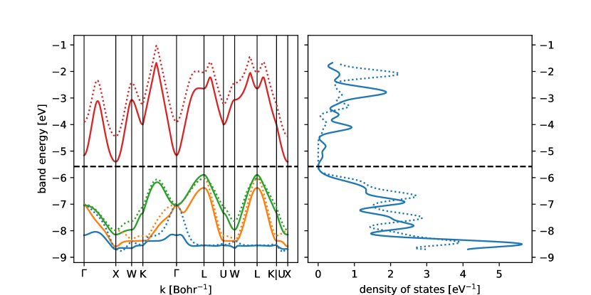
Figure 1: Band structure diagram (left) and the DOS (right) of AgI obtained at the 4c (full line) and 1c (dashed line) levels of theory with the PBE XC functional. The horizontal dashed black line separates the occupied and the vacant states, and was placed in the middle of the band gap. The path traversing high-symmetry $\bm{k}$-points in the reciprocal-space unit cell was chosen according to Ref. Setyawan and Curtarolo (2010). The figure was generated using Python matplotlib library Hunter (2007).

In order to alleviate the convergence problems described in Sec. IV.2 that are related to diffuse Gaussian-type functions in the atomic basis sets, we followed the common practice of removing the GTOs with exponents $<0.1$ from the original basis sets Geipel and He$\beta$ (1997); Peralta et al. (2005); Peintinger et al. (2013); Zhao et al. (2016). In this work, we deleted the most diffuse s- and p-type functions on Ag, and denoted the reduced basis by acronym “r” added in front of the original basis set name. During the numerical integration of the XC term, GTOs were considered to have a finite extent, defined as the radius of an atom-centered sphere outside of which values of the most diffuse Gaussian function are below a user-defined threshold. The extent of the original basis sets was 12.1 Å due to the diffuse functions on Ag. Using the truncated r-type basis sets reduced this extent to values between 7.4 and 7.8 Å. The GTO extent defined as in Ref. Watson et al. (2004) used in the multipole expansions of the Coulomb term had almost identical values.

Table 1 shows the results of our 4c and 1c calculations of the energy gaps for the Ag$X$ systems. Our values are compared with the results calculated using two different techniques Zhao et al. (2016): 2c method based on the X2C Hamiltonian and STOs, and the 4c LAPW method. The vertical (direct) band gaps are obtained at a set of special $\bm{k}$-points: $\Gamma$, L, and X. The band-structure diagram and the density of states (DOS) of AgI calculated at the 1c and 4c levels are depicted in Figure 1; DOS was obtained as $N(\varepsilon)\equiv\frac{1}{\mathcal{N}}\sum_{p\bm{k}}\delta(\varepsilon-\varepsilon_{p\bm{k}})$, where $\mathcal{N}$ is the total number of sampled $\bm{k}$ points, and the $\delta$-function was represented with a Gaussian with a standard deviation of 136 meV. These results show that the ionic Ag$X$ compounds are indirect semi-conductors, with the band gap occurring between the L and $\Gamma$ points for AgCl and AgBr, and between the L and X points for AgI. This agrees with the findings of previous studies Peralta et al. (2005); Zhao et al. (2016). All band gaps are significantly reduced when including relativistic effects, and Figure 1 reveals that this reduction is due to a large decrease in the energy of the entire conduction band. In Figure 1, we can also observe strong SOC splittings that occur within the valence bands. In particular, SOC lifts the degeneracy on the $\Gamma$-X and $\Gamma$-L lines, and for $\bm{k}=\Gamma$, the difference between the split energies equals to 1.13 eV. Overall, our results calculated with the DZ basis set agree well with those presented in Ref. Zhao et al. (2016); we reproduce the general trends as well as the difference between the relativistic and the nonrelativistic calculations.

Table 2: Nonrelativistic 1c energy band gaps of three-dimensional AgI calculated with a hierarchy of basis sets. All results are obtained with the PBE functional. Comparisons are made with non-relativistic literature values obtained using either STOs or plane waves, and are taken from Ref. Zhao et al. (2016).

AgI	Gap [eV]
basis	L–L	$\Gamma$–$\Gamma$	X–X	L–X
rDZ	5.12	3.28	3.58	1.62
rVDZ	4.87	3.30	3.60	1.62
rVTZ	4.66	3.74	3.50	1.56
rVQZ	4.01	3.21	3.56	1.59
DZ	3.99	3.11	3.54	1.59
VDZ	3.95	3.14	3.56	1.59
STO	3.91	3.14	3.56	1.60
LAPW	3.92	3.13	3.54	1.58

On the other hand, there is a notable discrepancy between the L–L direct gaps evaluated using the DZ and the rDZ basis sets, particularly for AgI. The fact that DZ results agree well with the STO and LAPW results in Ref. Zhao et al. (2016) indicates that the diffuse functions are of immense importance for the band structures of these systems, and should not be removed from the basis set. To further investigate the basis set effect, we conducted additional tests at the 1c level with various basis sets, and the results for band gaps of AgI are summarized in Table 2. In addition to the DZ basis set, we included the larger Dyall’s valence double-$\zeta$ (VDZ), as well as the hierarchical system of basis sets: reduced valence double-, triple-, and quadruple-$\zeta$ (rVDZ, rVTZ, rVQZ), with discarded the exponents smaller than $0.1$. The sequence of basis sets without the diffuse functions does not exhibit an apparent convergence, the $\Gamma$–$\Gamma$ gap deviates more from the reference results for larger basis sets. Acceptable agreement is reached only with the very large rVQZ. This issue does not appear for the original basis sets with diffuse exponents, and our results agree very well with those of Zhao et al. Zhao et al. (2016) already for DZ and VDZ. A similar observation was done by Zhao et al., who performed test calculations on AgCl with polarized double-$\zeta$ STOs, and the calculated band gaps differed marginally ($<0.1$ eV) from the results obtained with the large reduced polarized quadruple-$\zeta$ basis (rQZ4P) with eliminated diffuse s and p functions. In addition, this is in line with the findings of Te Velde and Baerends Te Velde and Baerends (1991) that a reasonable basis-set limit (with errors $<10^{-3}$ a.u. in cohesive energies per atom) can be reached for densely packed systems already with STOs of double-$\zeta$ quality, provided they contain polarization functions. Considering that GTOs and STOs only differ in the radial part, one would expect that a similar behavior should be seen also for GTOs. We have confirmed this observation, but only for the full original DZ basis set with diffuse exponents. Therefore, great care must be taken when adopting basis sets for solid-state calculations, and we do not generally recommend deleting diffuse exponents for heavy elements. Optimized solid-state GTOs have been developed by Peintinger et al. Peintinger et al. (2013) for the lighter elements of the periodic table, but this work needs to be extended to address the elements in the lower part of the periodic table as well.

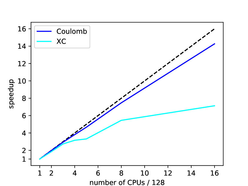
Figure 2: Speedup on the wall-clock time of the evaluation of the Coulomb and XC contributions to the Fock matrix in real space for 1 SCF cycle of the 4c AgI as a function of the number of CPUs used. The reference calculation was performed using 128 CPUs (4 nodes), and the largest calculation used 2048 CPUs (64 nodes). The dashed line denotes a hypothetical (linear) scaling of wall-clock time with given computational resources. The figure was generated using Python matplotlib library Hunter (2007).

Finally, we tested the parallel performance of our implementation with respect to the number of central processing units (CPUs) used. We conducted a series of 4c calculations on AgI with the DZ basis using two-socket computational nodes, where each socket consists of 16 physical cores. We used the calculation on four nodes (128 CPUs) as a reference. Figure 2 demonstrates near-ideal linear scaling with the number of processors of the NF Coulomb contributions to the Fock matrix and energy. The implementation remains efficient even when 64 nodes (2048 CPUs) are used. The evaluation of the XC contributions exhibits optimal scaling for a smaller number of nodes, but becomes less optimal beyond 1024 CPUs. However, absolute wall-clock times required to compute the XC contribution are considerably shorter than for the Coulomb terms. The remaining steps in the algorithm, such as the FF Coulomb contributions, Fourier transformation, matrix diagonalizations, and the DIIS, are negligible.

V.2 Honeycomb structures

To validate our method on systems displaying larger spin–orbit effects, we have also calculated the band structure of the heavier two-dimensional analogues of graphene: silicene and germanene. Both systems have been found to be stable in a low-buckled hexagonal geometry Liu et al. (2011), contrary to the truly planar graphene. In contrast to graphene, the buckled geometry of silicene and germanene enhances the SOC effect Liu et al. (2011). To compare our calculated band gaps with literature values, we used the geometries from Ref. Liu et al. (2011), and the nonrelativistic PBE functional Perdew et al. (1996). The integration grid for the XC contributions contained 80 radial points per atom, and Lebedev quadrature grid points of an adaptive size in the angular part Krack and Köster (1998). Reciprocal space integration was performed on a uniform grid of $31\times 31$ $\bm{k}$-points. We studied the effect of basis set on the band gap, and employed the uncontracted all-electron upob-TZVP Peintinger et al. (2013) and the hierarchy of systematically improved Dunning’s basis sets Wilson et al. (1999) (ucc-pVDZ, ucc-pVTZ, ucc-pVQZ).

Table 3: Band gaps of two-dimensional honeycomb structures at the fully relativistic (fr) 4c and nonrelativistic (nr) 1c level of theory using the PBE functional and various basis sets. Geometries are taken from Ref. Liu et al. (2011).

		Band gap [meV]
Method	Basis	Silicene	Germanene
nr	upob-TZVP	$0.026$	$0.028$
fr	upob-TZVP	$1.548$	$25.119$
fr	ucc-pVDZ	$1.596$	$24.296$
fr	ucc-pVTZ	$1.606$	$24.323$
fr	ucc-pVQZ	$1.607$	$24.342$
Ref. Liu et al. (2011)		$1.55$	$23.9$

Table 3 collects our calculated band gaps at the 1c and 4c levels of theory at the Dirac points ($\bm{k}=K$) of silicene and germanene. For comparison, we report in Table 3 also the results of Liu, Feng and Yao Liu et al. (2011) calculated using the relativistic pseudopotential PAW approach Dal Corso (2010). Since these graphene-like structures exhibit a quantum spin Hall effect Gmitra et al. (2009); Liu et al. (2011); Han et al. (2014), the existence of a nonzero gap is solely due to SOC. Hence, the nonrelativistic band gaps should then be strictly zero. The numbers in Table 3 do not display this feature exactly, but we attribute the very small values of the nonrelativistic gaps to numerical noise and the truncation of the expansion of the one-electron bases (finite basis effect). The convergence with respect to the basis limit is very fast — our ucc-pVDZ band gaps differ only marginally from the ucc-pVTZ and ucc-pVQZ results, whereas a larger discrepancy exists already between the ucc-pVDZ results and the results in Ref. Liu et al. (2011). Since our band gaps are obtained at the fully relativistic 4c level with the all-electron potential and well-converged basis, one can consider them as reference data. The small discrepancy between our 4c method and the previously reported 2c Pauli-type relativistic PAW method Dal Corso (2010) of Ref. Liu et al. (2011) can be attributed to the different treatment of relativity and the use of the pseudopotential approximation in the latter approach. We believe that these results demonstrate that the presented methodology opens a new possibility to study heavy-element-containing materials with promising technological applications, for instance in spintronic devices.

VI Conclusion and outlook

We have presented a first-principles full-potential relativistic method and its implementation for solving the 4c Dirac–Kohn–Sham equation for periodic systems employing a local basis composed of Gaussian-type orbitals. The proposed method accounts variationally for both scalar-relativistic as well as spin–orbit effects, allowing us to study solids across the entire periodic table in a uniform and consistent manner. The explicit built-in periodicity allows for a treatment of systems of arbitrary dimensionality without having to introduce nonphysical replicas of the systems studied in non-periodic dimensions. We formulated key principles of the method in the 4c Kramers-restricted framework, exploiting the time-reversal structure of operators in real and reciprocal space, and showed how to assemble the real-space Coulomb and exchange–correlation operators in this framework. We have discussed the conditionally-convergent electrostatic infinite lattice sums arising in studies of periodic systems, and we adopted the multipole expansion and an iterative renormalization procedure to calculate the lattice sums of the interaction tensor. To accelerate the calculations, some explicit two-electron integrals were neglected based on an efficient screening scheme, or approximated with a multipole expansion. We have analyzed the problem of inverse variational collapse that emerges in the 4c method if the employed basis set contains diffuse functions, and have suggested a means for avoiding the breakdown of the 4c SCF procedure. The method has been implemented in the 4c ReSpect res code, using the vectorized integral library InteRest int . Finally, we have validated this methodology on some exemplary calculations of three-dimensional silver halide crystals in their fcc phase, and two-dimensional honeycomb structures featuring the quantum spin Hall effect. Energy band gaps were calculated at various special $\bm{k}$-points. Overall, our results agreed very well with earlier published findings. Furthermore, we have demonstrated that the convergence with respect to the basis limit is possible for standard basis sets used for molecular calculations in quantum chemistry, without the need to modify the basis sets by removing the most diffuse exponents. We obtained very good cost–performance ratio of our hybrid OpenMP/MPI parallel implementation as we increased the number of used CPUs up to 2048.

The methodology presented in this paper holds promise in the computational study of solid-state materials. The 4c scheme is conceptually simpler and more transparent than approximate 2c techniques, and can be used to produce reference results to benchmark more approximate methods, and in this way increase confidence in approximate schemes and thus pave the way for computational studies of more complex materials. Furthermore, the full-potential formalism adopted here enables investigations of unique features of spin–orbit coupled materials, such as magnetic response properties and core-electron (X-ray) spectroscopy, where a full relativistic description is needed. We also believe that the method can prove valuable in a search for materials with non-trivial topological properties.

Appendix A Translational symmetry

In this appendix, we review some consequences of the translational symmetry on operators in various basis representations. We will here only be concerned with discrete translations, i.e. translations by an arbitrary integer-modulated lattice vector $\bm{m}$, defined by Eq. (5). Let $t_{\bm{m}}$ denote a translation operator for the lattice vector $\bm{m}$, defined by an application to a function $f$:

$$(t_{\bm{m}}f)(\bm{r})\equiv f(\bm{r}-\bm{m}).$$ (116)

An operator $A$ is translationally invariant iff it commutes with the translation operators for all lattice vectors $\bm{m}$ ($[\cdot,\cdot]$ denotes a commutator):

$$\left[A,t_{\bm{m}}\right]=0.$$ (117)

Clearly, the momentum operator $\bm{p}$, as well as the spin operator $\bm{\sigma}$ are translationally invariant. As a consequence, the composite operators $p^{2}/2$ (nonrelativistic kinetic energy) and $\bm{\sigma}\cdot\bm{p}$ are also translationally invariant. For this reason, we can omit the spin- and momentum-dependence of an operator $A$ from the following discussion without loss of generality. Let $A(\bm{r})$ be the coordinate representation of $A$. Translation invariance of $A$ [Eq. (117)] then requires

$$A(\bm{r}+\bm{m})=A(\bm{r}).$$ (118)

Matrix elements of $A$ expressed in the discrete real-space basis of Eq. (4) are obtained as

$$A_{\mu\bm{m},\mu^{\prime}\bm{m}^{\prime}}=\int_{\mathbb{R}^{3}}\chi^{\dagger}_{\mu\bm{m}}(\bm{r})A(\bm{r})\chi_{\mu^{\prime}\bm{m}^{\prime}}(\bm{r})d^{3}\bm{r}.$$ (119)

For any lattice vector $\bm{n}$, it follows, that

$$A_{\mu\bm{m},\mu^{\prime}\bm{m}^{\prime}}=A_{\mu\bm{m}+\bm{n},\mu^{\prime}\bm{m}^{\prime}+\bm{n}}=A_{\mu\bm{0},\mu^{\prime}\bm{m}^{\prime}-\bm{m}},$$ (120)

implying that the real-space matrix elements of translationally invariant operators have a Toeplitz structure. In addition, if the operator $A$ is Hermitian, then

$$A^{\dagger}_{\mu\bm{0},\mu^{\prime}\bm{m}}=A_{\mu^{\prime}\bm{0},\mu-\bm{m}},$$ (121)

where $A^{\dagger}$ denotes the Hermitian conjugate within the $4\times 4$ bispinor space.

Reciprocal-space elements of $A$ for $\bm{k},\bm{k}^{\prime}\in\mathcal{K}$ are acquired by using Eq. (6) together with Eq. (120):

$$A_{\mu\mu^{\prime}}(\bm{k},\bm{k}^{\prime})=\frac{1}{|\mathcal{K}|}\sum_{\bm{mm}^{\prime}}e^{-i\bm{k}\cdot{\bm{m}}}e^{i\bm{k}^{\prime}\cdot\bm{m}^{\prime}}A_{\mu\bm{0},\mu^{\prime}\bm{m}^{\prime}-\bm{m}}.$$

Changing the summation variables yields

$$A_{\mu\mu^{\prime}}(\bm{k},\bm{k}^{\prime}) =\delta(\bm{k}-\bm{k}^{\prime})A_{\mu\mu^{\prime}}(\bm{k}),$$ (122)

$$A_{\mu\mu^{\prime}}(\bm{k}) =\sum_{\bm{m}}e^{i\bm{k}\cdot{\bm{m}}}A_{\mu\bm{0},\mu^{\prime}\bm{m}},$$ (123)

where we have employed

$$\delta(\bm{k})\equiv\frac{1}{|\mathcal{K}|}\sum_{\bm{m}}e^{i\bm{k}\cdot{\bm{m}}},$$ (124)

which is the Fourier kernel representation of the Dirac delta function. Notice that the symmetry in Eq. (120) resulted in the block-diagonal reciprocal-space matrix [Eq. (122)]. This argument can also be reversed, i.e. any block-diagonal $\bm{k}$-space matrix will have a Toeplitz structure [Eq. (120)] in real space. We have applied this argument when constructing only the nonequivalent elements of the real-space density matrix in Eq. (23). Finally, the symmetry in Eq. (121) leads to matrices in the reciprocal space that are Hermitian for each $\bm{k}$ individually:

$$A^{\dagger}_{\mu\mu^{\prime}}(\bm{k})=A_{\mu^{\prime}\mu}(\bm{k}).$$ (125)

Therefore, provided that the Fock matrix in Eq. (14) satisfies the combined translational and Hermitian symmetry in Eq. (121), the eigenvalues $\varepsilon(\bm{k})$ in Eq. (11) are guaranteed to be real.

Translational symmetry allows us to assign finite expectation values of operators that naturally describe extensive properties, such as the kinetic energy of electrons. Beginning with a divergent expression for the expectation value of a translationally invariant one-electron operator $A$ (given that the density matrix is translationally invariant as well), we can write

$$\left\langle A\right\rangle =\sum_{\bm{mm}^{\prime}}\operatorname{Tr}\left[A_{\mu\bm{m},\mu^{\prime}\bm{m}^{\prime}}D^{\mu^{\prime}\bm{m}^{\prime},\mu\bm{m}}\right]$$

$$=\sum_{\bm{m}}1\sum_{\bm{m}^{\prime}}\operatorname{Tr}\left[A_{\mu\bm{0},\mu^{\prime}\bm{m}^{\prime}}D^{\mu^{\prime}\bm{m}^{\prime},\mu\bm{0}}\right],$$

where $\operatorname{Tr}$ denotes the trace in the $4\times 4$ bispinor space. If we employ the short-hand notation from Eq. (31), and realize, that $\sum_{\bm{m}}1\equiv N$ is the total (infinite) number of unit cells, we can calculate the expectation value of $A$ per unit cell in the thermodynamic limit ($N\rightarrow\infty$) as

$$\frac{\left\langle A\right\rangle}{N}=\operatorname{Tr}\left[A_{u}D^{\bar{u}}\right].$$ (126)

Appendix B Spherical multipole expansion

Here, we summarize the formulation of the spherical multipole expansion needed to evaluate the far-field contribution to the Coulomb operator. We follow the framework of Helgaker et al. Helgaker et al. (2000) and Watson et al. Watson et al. (2004) The Coulomb interaction operator $|\bm{r}_{1}-\bm{r}_{2}|^{-1}\equiv r_{12}^{-1}$ can be expanded (as a function of 6 variables) around an arbitrary center $(\bm{P},\bm{Q})$ into a spherical multipole expansion which takes the form

$$\frac{1}{r_{12}}=\sum_{l=0}^{\infty}\sum_{m=-l}^{l}\sum_{j=0}^{\infty}\sum_{k=-j}^{j}R^{lm}(\bm{r}_{1}-\bm{P})\Theta_{lm,jk}(\bm{Q}-\bm{P})R^{jk}(\bm{r}_{2}-\bm{Q}),$$ (127)

where

$$\Theta_{lm,jk}(\bm{R})=(-1)^{j}I^{*}_{l+j,m+k}(\bm{R}),$$ (128)

is the interaction tensor, $R^{lm}(\bm{r})$ and $I_{lm}(\bm{r})$ are the scaled regular and scaled irregular solid harmonics, respectively, defined as

$$R^{lm}(\bm{r}) =\frac{1}{\sqrt{(l-m)!(l+m)!}}r^{l}C_{lm}(\vartheta,\varphi),$$ (129)

$$I_{lm}(\bm{r}) =\sqrt{(l-m)!(l+m)!}r^{-l-1}C_{lm}(\vartheta,\varphi).$$ (130)

Here $C_{lm}(\vartheta,\varphi)$ are eigenfunctions of the angular momentum operators $L^{2},L_{z}$, namely, the spherical harmonics in Racah’s normalization, obtained from the conventional spherical harmonics $Y_{lm}(\vartheta,\varphi)$ as

$$C_{lm}(\vartheta,\varphi)=\sqrt{\frac{4\pi}{2l+1}}Y_{lm}(\vartheta,\varphi).$$ (131)

We shall use the compact matrix notation

$$\frac{1}{r_{12}}=R^{T}(\bm{r}_{1}-\bm{P})\Theta(\bm{Q}-\bm{P})R(\bm{r}_{2}-\bm{Q}),$$ (132)

where $R$ is a vector and $\Theta$ is a matrix defined by their respective elements $R^{lm}$ and $\Theta_{lm,jk}$. The series in Eq. (132) is convergent for all points $(\bm{r}_{1},\bm{r}_{2})$ that satisfy the condition

$$|\bm{r}_{1}-\bm{r}_{2}+\bm{Q}-\bm{P}|<|\bm{Q}-\bm{P}|.$$ (133)

The scaled regular and irregular solid harmonics have the following properties ($\lambda\in\mathbb{R}$ is an arbitrary scaling factor):

$$R^{l-m}(\bm{r}) =(-1)^{m}R^{lm*}(\bm{r}),$$ (134a)

$$I_{l-m}(\bm{r}) =(-1)^{m}I_{lm}^{*}(\bm{r}),$$ (134b)

$$R^{lm}(\lambda\bm{r}) =\lambda^{l}R^{lm}(\bm{r}),$$ (134c)

$$I_{lm}(\lambda\bm{r}) =\frac{1}{|\lambda|}\frac{1}{\lambda^{l}}I_{lm}(\bm{r}).$$ (134d)

The regular solid harmonics obey the addition theorem

$$R^{lm}(\bm{r}-\bm{P})=\sum_{j=0}^{l}\sum_{k=-j}^{j}R_{l-j,m-k}(-\bm{P})R^{jk}(\bm{r}),$$ (135)

which can be written in the following matrix form

$$R(\bm{r}-\bm{P})=W(\bm{P})R(\bm{r}),$$ (136)

where $W$ is the translation tensor, its elements defined as

$$W_{lm,jk}(\bm{P})=R_{l-j,m-k}(-\bm{P}).$$ (137)

The translation tensor $W$ can be used to evaluate the regular solid harmonics for shifted arguments. Moreover, we can apply Eq. (136) to derive a similar rule for the interaction tensor. Multipole expansions of $r_{12}^{-1}$ expanded around 2 different centers $(\bm{P},\bm{Q})$ and $(\bar{\bm{P}},\bar{\bm{Q})}$ must coincide, so that

$$\frac{1}{r_{12}} =R^{T}(\bm{r}_{1}-\bm{P})\Theta(\bm{Q}-\bm{P})R(\bm{r}_{2}-\bm{Q})$$

$$=R^{T}(\bm{r}_{1}-\bar{\bm{P}})\Theta(\bar{\bm{Q}}-\bar{\bm{P}})R(\bm{r}_{2}-\bar{\bm{Q}}).$$

Applying the addition theorem [Eq. (136)], we identify

$$\Theta(\bm{Q}-\bm{P})=W^{T}(\bar{\bm{P}}-\bm{P})\Theta(\bar{\bm{Q}}-\bar{\bm{P}})W(\bar{\bm{Q}}-\bm{Q}).$$ (138)

Using $W(\bm{0})=\mathbb{I}$, and setting $\bar{\bm{P}}=\bm{P}$ and $\bar{\bm{Q}}=\bm{P}+\bm{Q}$ in Eq. (138), we obtain the corollary

$$\Theta(\bm{Q}-\bm{P})=\Theta(\bm{Q})W(\bm{P}).$$ (139)

In the present implementation, we avoid using complex numbers for multipole expansions by expressing interaction and translation tensors in terms of the real (regular and irregular) solid harmonics, which we construct from recurrence equations (see Ref. Helgaker et al. (2000)) and we do therefore not evaluate the zero imaginary part of the real-valued Coulomb $r_{12}^{-1}$ operator.

Appendix C Lattice sum of interaction tensors

Here we prove the recurrence relation in Eq. (89), establishing a rapidly convergent scheme for the computation of lattice sums of spherical interaction tensors. Let us begin by fragmenting the far-field (FF) into layers FF_r as follows: Let the near-field (NF) be a block consisting of unit cells with indices $n^{i}=-N_{i},\ldots,N_{i}$ for each of the periodic dimensions $i=1,\ldots,d$. For generic noncubic lattices, such an object has a diamondlike shape. The first layer of the far-field, FF₁, envelopes the NF by placing supercells in all directions, each supercell having as many unit cells as the NF itself. The process is then repeated for the next layer of the far-field, FF₂, with the exception that the supercell now contains all unit cells in both NF and FF₁, as depicted in the following scheme:

$$\ldots\mid\underbrace{\overbrace{-3N_{i}-1\ldots-N_{i}-1}^{\text{FF}_{1}}}_{2N_{i}+1}\mid\underbrace{\overbrace{-N_{i}\ldots-1}^{\text{NF}}\boxed{0}\overbrace{1\ldots N_{i}}^{\text{NF}}}_{2N_{i}+1}\mid\underbrace{\overbrace{N_{i}+1\ldots 3N_{i}+1}^{\text{FF}_{1}}}_{2N_{i}+1}\mid\underbrace{\overbrace{3N_{i}+2\ldots 9N_{i}+4}^{\text{FF}_{2}}}_{2(3N_{i}+1)+1}\mid\ldots$$ (140)

Let $N_{ir}$ denote the upper extent of the far-field layer $r$ in the direction $i$, i.e. it is the index of the unit cell that is the farthest from the center $0$. Then $N_{ir}$ satisfies the following recurrence relations ($r=0$ labels the NF)

$$\begin{split}N_{i0}&=N_{i},\\ N_{ir+1}&=3N_{ir}+1,\end{split}$$ (141)

which have the solution

$$N_{ir}=\frac{(2N_{i}+1)3^{r}-1}{2}.$$ (142)

The number of unit cells in layer $r$ is given by

$$|\text{FF}_{r}|=3^{d(r-1)}(3^{d}-1)|\text{NF}|,$$ (143)

where $|X|$ denotes the number of elements of $X$. From Eq. (143), we can see that the sizes of the layers form a geometric sequence. Therefore, the partitioning in Eq. (140) divides the space into regions that become exponentially larger with each new layer. Formally, we define FF_r as

$$\text{FF}_{r}=\left\{(n^{1}\ldots n^{d})\in\mathbb{Z}^{d};1\leq\max_{i=1\ldots d}\left(\frac{|n^{i}|-1}{N_{ir-1}}\right)\leq 3\right\}.$$ (144)

The overall far-field is then given by the union

$$\text{FF}=\bigcup_{r=1}^{\infty}\text{FF}_{r},$$ (145)

and the lattice sum in Eq. (83) becomes

$$\Lambda=\sum_{\bm{n}\in\text{FF}}\Theta(\bm{n})=\lim_{t\rightarrow\infty}\sum_{r=1}^{t}\sum_{n\in\text{FF}_{r}}\Theta(n^{i}\bm{a}_{i}),$$

where we have abbreviated the summation indices as $n=(n^{1}\ldots n^{d})$. It follows, that the lattice sum is obtained as a limit of partial sums

$$\Lambda =\lim_{t\rightarrow\infty}\Lambda^{t},$$ (146)

$$\Lambda^{t} =\sum_{r=1}^{t}\sum_{n\in\text{FF}_{r}}\Theta(n^{i}\bm{a}_{i}).$$ (147)

Let us consider the term $t+1$:

$$\Lambda^{t+1} =\Lambda^{1}+\sum_{r=2}^{t+1}\sum_{n\in\text{FF}_{r}}\Theta(n^{i}\bm{a}_{i})$$

$$=\Lambda^{1}+\sum_{r=1}^{t}\sum_{n\in\text{FF}_{r+1}}\Theta(n^{i}\bm{a}_{i}).$$ (148)

The following identity relates the two sums over different layers of the far-field

$$\sum_{n\in\text{FF}_{r+1}}\Theta(n^{i}\bm{a}_{i})=\sum_{n\in\text{FF}_{r}}\sum_{\mu\in\mathcal{P}}\Theta\left((3n^{i}-\mu^{i})\bm{a}_{i}\right),$$ (149)

where $\mathcal{P}$ is the Cartesian power

$$\mathcal{P}=\left\{-1,0,1\right\}^{d},$$

for $d=3,\mathcal{P}=\left\{(\pm 1,\pm 1,\pm 1),(\pm 1,\pm 1,0),\ldots\right\}$ and contains the reference unit cell and all its 26 nearest neighbours.

Up to this point, the proof has been of a general nature — we did not need to specify $\Theta$ or use its properties. However, in order to obtain an applicable recursive formulation, we need to express the term $\Lambda^{t+1}$ via the previous terms. To proceed, we therefore apply the addition theorem in Eq. (139), factorizing the interaction tensor as

$$\Theta\left((3n^{i}-\mu^{i})\bm{a}_{i}\right) =\Theta\left(3n^{i}\bm{a}_{i}\right)W\left(\mu^{i}\bm{a}_{i}\right)$$

$$\equiv\mathcal{U}\left[\Theta\left(n^{i}\bm{a}_{i}\right)\right]W\left(\mu^{i}\bm{a}_{i}\right),$$

where $W$ is the translation tensor [Eq. (137)], and where we have defined the scaling operator $\mathcal{U}$ as

$$\mathcal{U}\left[\Theta_{lm,jk}(\bm{n})\right]\equiv\Theta_{lm,jk}(3\bm{n})=\frac{1}{3^{l+j+1}}\Theta_{lm,jk}(\bm{n}).$$ (150)

Here we applied the scaling property of the irregular solid harmonics [Eq. (134d)]. Returning to Eq. (148), this leads to

$$\Lambda^{t+1} =\Lambda^{1}+\sum_{r=1}^{t}\sum_{n\in\text{FF}_{r}}\sum_{\mu\in\mathcal{P}}\Theta\left((3n^{i}-\mu^{i})\bm{a}_{i}\right)$$

$$=\Lambda^{1}+\mathcal{U}\left[\sum_{r=1}^{t}\sum_{n\in\text{FF}_{r}}\Theta\left(n^{i}\bm{a}_{i}\right)\right]\sum_{\mu\in\mathcal{P}}W\left(\mu^{i}\bm{a}_{i}\right).$$

If we define the aggregate translation matrix

$$\mathcal{W}=\sum_{\mu\in\mathcal{P}}W\left(\mu^{i}\bm{a}_{i}\right)\equiv\sum_{\mu^{1}\ldots\mu^{d}=-1}^{1}W(\mu^{i}\bm{a}_{i}),$$ (151)

then

$$\Lambda^{t+1}=\Lambda^{1}+\mathcal{U}\left(\Lambda^{t}\right)\mathcal{W},$$ (152)

which completes the proof.

References

- Christensen and Seraphin (1971) N. E. Christensen and B. Seraphin, Phys. Rev. B 4, 3321 (1971).
- Pincherle (1933) L. Pincherle, Il Nuovo Cimento (1924-1942) 10, 344 (1933).
- Mayers (1957) D. Mayers, Proc. R. Soc. A 241, 93 (1957).
- Christensen et al. (1986) N. Christensen, S. Satpathy, and Z. Pawlowska, Phys. Rev. B 34, 5977 (1986).
- Söhnel et al. (2001) T. Söhnel, H. Hermann, and P. Schwerdtfeger, Angew. Chem. Int. Ed. 40, 4381 (2001).
- Pyykko (1988) P. Pyykko, Chem. Rev. 88, 563 (1988).
- Christensen and Kollar (1983) N. Christensen and J. Kollar, Solid State Commun. 46, 727 (1983).
- Ahuja et al. (2011) R. Ahuja, A. Blomqvist, P. Larsson, P. Pyykkö, and P. Zaleski-Ejgierd, Phys. Rev. Lett. 106, 018301 (2011).
- Calvo et al. (2013) F. Calvo, E. Pahl, M. Wormit, and P. Schwerdtfeger, Angew. Chem. Int. Ed. 52, 7583 (2013).
- Dresselhaus (1955) G. Dresselhaus, Phys. Rev. 100, 580 (1955).
- Broido and Sham (1985) D. Broido and L. Sham, Phys. Rev. B 31, 888 (1985).
- Rashba and Sherman (1988) E. Rashba and E. Y. Sherman, Phys. Lett. A 129, 175 (1988).
- Zhu et al. (2011) Z. Zhu, Y. Cheng, and U. Schwingenschlögl, Phys. Rev. B 84, 153402 (2011).
- Heine (2014) T. Heine, Acc. Chem. Res. 48, 65 (2014).
- Rasmussen and Thygesen (2015) F. A. Rasmussen and K. S. Thygesen, J. Phys. Chem. C 119, 13169 (2015).
- Xu et al. (2014) X. Xu, W. Yao, D. Xiao, and T. F. Heinz, Nat. Phys. 10, 343 (2014).
- Rashba (2000) E. Rashba, Phys. Rev. B 62, R16267 (2000).
- Wolf et al. (2001) S. Wolf, D. Awschalom, R. Buhrman, J. Daughton, S. Von Molnar, M. Roukes, A. Y. Chtchelkanova, and D. Treger, Science 294, 1488 (2001).
- Žutić et al. (2004) I. Žutić, J. Fabian, and S. D. Sarma, Rev. Mod. Phys. 76, 323 (2004).
- Kane and Mele (2005) C. L. Kane and E. J. Mele, Phys. Rev. Lett. 95, 226801 (2005).
- Hasan and Kane (2010) M. Z. Hasan and C. L. Kane, Rev. Mod. Phys. 82, 3045 (2010).
- Sinova et al. (2004) J. Sinova, D. Culcer, Q. Niu, N. Sinitsyn, T. Jungwirth, and A. MacDonald, Phys. Rev. Lett. 92, 126603 (2004).
- Sinova et al. (2015) J. Sinova, S. O. Valenzuela, J. Wunderlich, C. Back, and T. Jungwirth, Rev. Mod. Phys. 87, 1213 (2015).
- Kou et al. (2017) L. Kou, Y. Ma, Z. Sun, T. Heine, and C. Chen, J. Phys. Chem. Lett. 8, 1905 (2017).
- Gmitra et al. (2009) M. Gmitra, S. Konschuh, C. Ertler, C. Ambrosch-Draxl, and J. Fabian, Phys. Rev. B 80, 235431 (2009).
- Liu et al. (2011) C.-C. Liu, W. Feng, and Y. Yao, Phys. Rev. Lett. 107, 076802 (2011).
- Xu et al. (2013) Y. Xu, B. Yan, H.-J. Zhang, J. Wang, G. Xu, P. Tang, W. Duan, and S.-C. Zhang, Phys. Rev. Lett. 111, 136804 (2013).
- Han et al. (2014) W. Han, R. K. Kawakami, M. Gmitra, and J. Fabian, Nat. Nanotechnol. 9, 794 (2014).
- Hermann et al. (2010) A. Hermann, J. Furthmüller, H. W. Gäggeler, and P. Schwerdtfeger, Phys. Rev. B 82, 155116 (2010).
- Bradlyn et al. (2017) B. Bradlyn, L. Elcoro, J. Cano, M. Vergniory, Z. Wang, C. Felser, M. Aroyo, and B. A. Bernevig, Nature 547, 298 (2017).
- Bansil et al. (2016) A. Bansil, H. Lin, and T. Das, Rev. Mod. Phys. 88, 021004 (2016).
- Hohenberg and Kohn (1964) P. Hohenberg and W. Kohn, Phys. Rev. 136, B864 (1964).
- Kohn and Sham (1965) W. Kohn and L. J. Sham, Phys. Rev. 140, A1133 (1965).
- Sakuma et al. (2011) R. Sakuma, C. Friedrich, T. Miyake, S. Blügel, and F. Aryasetiawan, Phys. Rev. B 84, 085144 (2011).
- Scherpelz et al. (2016) P. Scherpelz, M. Govoni, I. Hamada, and G. Galli, J. Chem. Theory Comput. 12, 3523 (2016).
- Vanderbilt (1990) D. Vanderbilt, Phys. Rev. B 41, 7892 (1990).
- Troullier and Martins (1991) N. Troullier and J. L. Martins, Phys. Rev. B 43, 1993 (1991).
- Hangele et al. (2012) T. Hangele, M. Dolg, M. Hanrath, X. Cao, and P. Schwerdtfeger, J. Chem. Phys. 136, 214105 (2012).
- Kim et al. (2010) J. Kim, D. S. Middlemiss, N. A. Chernova, B. Y. Zhu, C. Masquelier, and C. P. Grey, J. Am. Chem. Soc. 132, 16825 (2010).
- Takada (1966) S. Takada, Prog. Theor. Phys. 36, 224 (1966).
- Strange et al. (1984) P. Strange, J. Staunton, and B. L. Gyorffy, J. Phys. C 17, 3355 (1984).
- Wang et al. (1992) X. Wang, X.-G. Zhang, W. Butler, G. Stocks, and B. Harmon, Phys. Rev. B 46, 9352 (1992).
- Der Kellen and Freeman (1996) S. B. Der Kellen and A. Freeman, Phys. Rev. B 54, 11187 (1996).
- Slater (1937) J. C. Slater, Phys. Rev. 51, 846 (1937).
- Loucks (1965) T. Loucks, Phys. Rev. 139, A1333 (1965).
- Mattheiss (1966) L. Mattheiss, Phys. Rev. 151, 450 (1966).
- Andersen (1975) O. K. Andersen, Phys. Rev. B 12, 3060 (1975).
- Sjöstedt et al. (2000) E. Sjöstedt, L. Nordström, and D. Singh, Solid State Commun. 114, 15 (2000).
- Christensen (1978) N. Christensen, J. Phys. F 8, L51 (1978).
- Godreche (1982) C. Godreche, J. Magn. Magn. Mater. 29, 262 (1982).
- Ebert (1988) H. Ebert, Phys. Rev. B 38, 9390 (1988).
- Ebert et al. (1988) H. Ebert, P. Strange, and B. L. Gyorffy, J. Appl. Phys. 63, 3052 (1988).
- MacDonald et al. (1980) A. MacDonald, W. Picket, and D. Koelling, J. Phys. C 13, 2675 (1980).
- Wimmer et al. (1981) E. Wimmer, H. Krakauer, M. Weinert, and A. Freeman, Phys. Rev. B 24, 864 (1981).
- Schwarz et al. (2002) K. Schwarz, P. Blaha, and G. K. Madsen, Comput. Phys. Commun. 147, 71 (2002).
- Blaha et al. (2001) P. Blaha, K. Schwarz, G. Madsen, D. Kvasnicka, and J. Luitz, “wien2k, An Augmented Plane Wave + Local Orbitals Program for Calculating Crystal Properties,” http://susi.theochem.tuwien.ac.at/ (Karlheinz Schwarz, Techn. UniversitatWien, Austria, 2001).
- Kurz et al. (2004) P. Kurz, F. Förster, L. Nordström, G. Bihlmayer, and S. Blügel, Phys. Rev. B 69, 024415 (2004).
- Blaha et al. (1992) P. Blaha, D. Singh, P. Sorantin, and K. Schwarz, Phys. Rev. B 46, 1321 (1992).
- Nordström et al. (2000) L. Nordström, J. Wills, P. H. Andersson, P. Söderlind, and O. Eriksson, Phys. Rev. B 63, 035103 (2000).
- Kuneš et al. (2001) J. Kuneš, P. Novak, R. Schmid, P. Blaha, and K. Schwarz, Phys. Rev. B 64, 153102 (2001).
- Carrier and Wei (2004) P. Carrier and S.-H. Wei, Phys. Rev. B 70, 035212 (2004).
- Huhn and Blum (2017) W. P. Huhn and V. Blum, Phys. Rev. Mater. 1, 033803 (2017).
- Blöchl (1994) P. E. Blöchl, Phys. Rev. B 50, 17953 (1994).
- Kresse and Joubert (1999) G. Kresse and D. Joubert, Phys. Rev. B 59, 1758 (1999).
- Dal Corso (2010) A. Dal Corso, Phys. Rev. B 82, 075116 (2010).
- Suzuki and Nakao (2000) S. Suzuki and K. Nakao, J. Phys. Soc. Jpn. 69, 532 (2000).
- Blum et al. (2009) V. Blum, R. Gehrke, F. Hanke, P. Havu, V. Havu, X. Ren, K. Reuter, and M. Scheffler, Comput. Phys. Commun. 180, 2175 (2009).
- Suzuki and Nakao (1999) S. Suzuki and K. Nakao, J. Phys. Soc. Jpn. 68, 1982 (1999).
- Koepernik and Eschrig (1999) K. Koepernik and H. Eschrig, Phys. Rev. B 59, 1743 (1999).
- Opahle (2001) I. Opahle, Dichtefunktionalberechnungen für Seltenerd- und Übergangsmetall-Verbindungen, Ph.D. thesis, University of Technology Dresden (2001).
- Eschrig et al. (2004) H. Eschrig, M. Richter, and I. Opahle, in Theoretical and computational chemistry, Vol. 14, edited by P. Schwerdtfeger (Elsevier, 2004) Chap. 12, pp. 723–776.
- Philipsen et al. (1997) P. Philipsen, E. Van Lenthe, J. Snijders, and E. Baerends, Phys. Rev. B 56, 13556 (1997).
- Philipsen and Baerends (2000) P. Philipsen and E. Baerends, Phys. Rev. B 61, 1773 (2000).
- Zhao et al. (2016) R. Zhao, Y. Zhang, Y. Xiao, and W. Liu, J. Chem. Phys. 144, 044105 (2016).
- Geipel and He (1997) N. J. Geipel and B. A. He, Chem. Phys. Lett. 273, 62 (1997).
- Peralta et al. (2005) J. E. Peralta, J. Uddin, and G. E. Scuseria, J. Chem. Phys. 122, 084108 (2005).
- Wang and Callaway (1974) C.-p. S. Wang and J. Callaway, Phys. Rev. B 9, 4897 (1974).
- Mainkar et al. (1996) N. Mainkar, D. A. Browne, and J. Callaway, Phys. Rev. B 53, 3692 (1996).
- Jones et al. (2000) M. Jones, J. Boettger, R. Albers, and D. Singh, Phys. Rev. B 61, 4644 (2000).
- Boettger (2000) J. Boettger, Phys. Rev. B 62, 7809 (2000).
- Soven (1965) P. Soven, Phys. Rev. 137, A1706 (1965).
- Goedecker (1999) S. Goedecker, Rev. Mod. Phys. 71, 1085 (1999).
- Miró et al. (2014) P. Miró, M. Audiffred, and T. Heine, Chem. Soc. Rev. 43, 6537 (2014).
- (84) ReSpect 5.0.1 (2018), relativistic spectroscopy DFT program of authors M. Repisky, S. Komorovsky, V. G. Malkin, O. L. Malkina, M. Kaupp, K. Ruud, with contributions from R. Bast, R. Di Remigio, U. Ekstrom, M. Kadek, S. Knecht, L. Konecny, E. Malkin, I. Malkin Ondik (http://www.respectprogram.org/).
- Konecny et al. (2018) L. Konecny, M. Kadek, S. Komorovsky, K. Ruud, and M. Repisky, J. Chem. Phys. 149, 204104 (2018).
- (86) M. Repisky, S. Komorovsky, and K. Ruud, (in preparation).
- Pisani and Dovesi (1980) C. Pisani and R. Dovesi, Int. J. Quantum Chem. 17, 501 (1980).
- Dovesi et al. (1983) R. Dovesi, C. Pisani, C. Roetti, and V. Saunders, Phys. Rev. B 28, 5781 (1983).
- Towler et al. (1996) M. D. Towler, A. Zupan, and M. Causà, Comput. Phys. Commun. 98, 181 (1996).
- Łazarski et al. (2015) R. Łazarski, A. M. Burow, and M. Sierka, J. Chem. Theory Comput. 11, 3029 (2015).
- Boys (1950) S. F. Boys, Proc. R. Soc. A 200, 542 (1950).
- Obara and Saika (1986) S. Obara and A. Saika, J. Chem. Phys. 84, 3963 (1986).
- Stanton and Havriliak (1984) R. E. Stanton and S. Havriliak, J. Chem. Phys. 81, 1910 (1984).
- Dirac (1928) P. A. Dirac, Proc. R. Soc. A 117, 610 (1928).
- Kutzelnigg (1984) W. Kutzelnigg, Int. J. Quantum Chem. 25, 107 (1984).
- Saue and Helgaker (2002) T. Saue and T. Helgaker, J. Comput. Chem. 23, 814 (2002).
- Komorovsky et al. (2008) S. Komorovsky, M. Repisky, O. L. Malkina, V. G. Malkin, I. Malkin Ondik, and M. Kaupp, J. Chem. Phys. 128, 104101 (2008).
- (98) InteRest (2018), an integral library for relativistic quantum chemistry of M. Repisky.
- Stolarczyk and Piela (1982) L. Z. Stolarczyk and L. Piela, Int. J. Quantum Chem. 22, 911 (1982).
- Ohnishi and Hirata (2012) Y. Ohnishi and S. Hirata, Chem. Phys. 401, 152 (2012).
- Aucar et al. (1995) G. Aucar, H. A. Jensen, and J. Oddershede, Chem. Phys. Lett. 232, 47 (1995).
- Saue (1996) T. Saue, Principles and Applications of Relativistic Molecular Calculations, Ph.D. thesis, University of Oslo (1996).
- Saue et al. (1997) T. Saue, K. Fægri, T. Helgaker, and O. Gropen, Mol. Phys. 91, 937 (1997).
- Komorovsky et al. (2016) S. Komorovsky, M. Repisky, and L. Bučinský, Phys. Rev. A 94, 052104 (2016).
- Dyall and Faegri (2007) K. G. Dyall and K. Faegri, Introduction to relativistic quantum chemistry (Oxford University Press, New York, 2007) pp. 92–97.
- Dyall (1994) K. G. Dyall, J. Chem. Phys. 100, 2118 (1994).
- Piela and Stolarczyk (1982) L. Piela and L. Z. Stolarczyk, Chem. Phys. Lett. 86, 195 (1982).
- Redlack and Grindlay (1975) A. Redlack and J. Grindlay, J. Phys. Chem. Solids 36, 73 (1975).
- de Leeuw et al. (1980) S. W. de Leeuw, J. W. Perram, and E. R. Smith, Proc. R. Soc. A 373, 27 (1980).
- Watson et al. (2004) M. A. Watson, P. Sałek, P. Macak, and T. Helgaker, J. Chem. Phys. 121, 2915 (2004).
- Helgaker et al. (2000) T. Helgaker, P. Jorgensen, and J. Olsen, Molecular electronic-structure theory (John Wiley & Sons, Chichester, 2000) pp. 405–416.
- Nijboer and De Wette (1957) B. R. A. Nijboer and F. W. De Wette, Physica 23, 309 (1957).
- Berman and Greengard (1994) C. L. Berman and L. Greengard, J. Math. Phys. 35, 6036 (1994).
- Kudin and Scuseria (2004) K. N. Kudin and G. E. Scuseria, J. Chem. Phys. 121, 2886 (2004).
- White et al. (1994) C. A. White, B. G. Johnson, P. M. Gill, and M. Head-Gordon, Chem. Phys. Lett. 230, 8 (1994).
- Kudin and Scuseria (1998) K. N. Kudin and G. E. Scuseria, Chem. Phys. Lett. 283, 61 (1998).
- Kantorovich and Tupitsyn (1999) L. Kantorovich and I. Tupitsyn, J. Phys. Condens. Matter 11, 6159 (1999).
- Becke (1988a) A. D. Becke, Phys. Rev. A 38, 3098 (1988a).
- Perdew et al. (1992) J. P. Perdew, J. A. Chevary, S. H. Vosko, K. A. Jackson, M. R. Pederson, D. J. Singh, and C. Fiolhais, Phys. Rev. B 46, 6671 (1992).
- Becke (1988b) A. D. Becke, J. Chem. Phys. 88, 2547 (1988b).
- Löwdin (1967) P.-O. Löwdin, Rev. Mod. Phys. 39, 259 (1967).
- (122) XCFun (2010), a library of DFT exchange-correlation functionals of U. Ekström and contributors (https://github.com/dftlibs/xcfun).
- Visscher and Dyall (1997) L. Visscher and K. G. Dyall, At. Data Nucl. Data Tables 67, 207 (1997).
- Pulay (1980) P. Pulay, Chem. Phys. Lett. 73, 393 (1980).
- Pulay (1982) P. Pulay, J. Comput. Chem. 3, 556 (1982).
- Kudin (2000) K. N. Kudin, Linear Scaling Density Functional Theory with Gaussian Orbitals and Periodic Boundary Conditions, Ph.D. thesis, Rice University (2000).
- Maschio (2018) L. Maschio, Theor. Chem. Acc. 137, 60 (2018).
- Suhai et al. (1982) S. Suhai, P. Bagus, and J. Ladik, Chem. Phys. 68, 467 (1982).
- Kudin and Scuseria (2000) K. N. Kudin and G. E. Scuseria, Phys. Rev. B 61, 16440 (2000).
- Jacquemin et al. (2002) D. Jacquemin, J. G. Fripiat, and B. Champagne, Int. J. Quantum Chem. 89, 452 (2002).
- Peintinger et al. (2013) M. F. Peintinger, D. V. Oliveira, and T. Bredow, J. Comput. Chem. 34, 451 (2013).
- Ayenew (2000) M. Ayenew, Bound States in the Dirac Equation, M.S. thesis, Addis Ababa University (2000).
- Schwerdtfeger et al. (2015) P. Schwerdtfeger, L. F. Pašteka, A. Punnett, and P. O. Bowman, Nucl. Phys. A 944, 551 (2015).
- Quiney et al. (1987) H. Quiney, I. Grant, and S. Wilson, Phys. Scr. 36, 460 (1987).
- Shabaev et al. (2004) V. Shabaev, I. Tupitsyn, V. Yerokhin, G. Plunien, and G. Soff, Phys. Rev. Lett. 93, 130405 (2004).
- Sun et al. (2011) Q. Sun, W. Liu, and W. Kutzelnigg, Theor. Chem. Acc. 129, 423 (2011).
- Saue (2011) T. Saue, ChemPhysChem 12, 3077 (2011).
- Perdew et al. (1996) J. P. Perdew, K. Burke, and M. Ernzerhof, Phys. Rev. Lett. 77, 3865 (1996).
- Dyall (1998) K. G. Dyall, Theor. Chem. Acc. 99, 366 (1998).
- Dyall (2002a) K. G. Dyall, Theor. Chem. Acc. 108, 365 (2002a).
- Dyall (2002b) K. G. Dyall, Theor. Chem. Acc. 108, 335 (2002b).
- Dyall (2006) K. G. Dyall, Theor. Chem. Acc. 115, 441 (2006).
- Dyall (2007) K. G. Dyall, Theor. Chem. Acc. 117, 483 (2007).
- Setyawan and Curtarolo (2010) W. Setyawan and S. Curtarolo, Comput. Mater. Sci. 49, 299 (2010).
- Hunter (2007) J. Hunter, Comput. Sci. Eng. 9, 90 (2007).
- Te Velde and Baerends (1991) G. Te Velde and E. Baerends, Phys. Rev. B 44, 7888 (1991).
- Krack and Köster (1998) M. Krack and A. M. Köster, J. Chem. Phys. 108, 3226 (1998).
- Wilson et al. (1999) A. K. Wilson, D. E. Woon, K. A. Peterson, and T. H. Dunning Jr, J. Chem. Phys. 110, 7667 (1999).