Modeling and Control of Soft Robots Using the Koopman Operator and Model Predictive Control

Abstract

Controlling soft robots with precision is a challenge due in large part to the difficulty of constructing models that are amenable to model-based control design techniques. Koopman operator theory offers a way to construct explicit linear dynamical models of soft robots and to control them using established model-based linear control methods. This method is data-driven, yet unlike other data-driven models such as neural networks, it yields an explicit control-oriented linear model rather than just a “black-box” input-output mapping. This work describes this Koopman-based system identification method and its application to model predictive controller design. A model and MPC controller of a pneumatic soft robot arm is constructed via the method, and its performance is evaluated over several trajectory following tasks in the real-world. On all of the tasks, the Koopman-based MPC controller outperforms a benchmark MPC controller based on a linear state-space model of the same system.

I Introduction

Soft robots have bodies made out of intrinsically soft and/or compliant materials. This inherent softness enables them to safely interact with delicate objects, and to passively adapt their shape to unstructured environments [26]. Such traits are desirable for robotic applications that demand safe human-robot interaction such as wearable robots, in-home assistive robots, and medical robots. Unfortunately, the soft bodies of these robots also impose modeling and control challenges, which have restricted their functionality to date. While many novel soft devices such as soft grippers [13], crawlers [32], and swimmers [16] exploit the flexibility of their bodies to achieve coarse behaviors such as grasping and locomotion, they do not exhibit precise control capabilities.

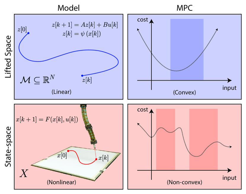
Figure 1: A nonlinear dynamical system (bottom-left) has a linear representation in the lifted space made up of all real-valued functions (top-left). While a model predictive controller (MPC) designed for the nonlinear system in state-space requires solving a non-convex optimization problem to choose inputs at each time-step (bottom-right), this problem is convex for an MPC controller designed for the lifted linear system (top-right). This paper develops a data-driven method to construct such a lifted model representation for soft robotic systems in the presence of outliers and a to construct a convex, model-based control design technique for such systems.

The challenge in constructing such precise control techniques is due in large part to the difficulty of devising models of soft robots that are amenable to model-based control design techniques. Consider for instance a rigid-bodied robotic system that is made up of rigid links connected together by discrete joints. Since joint displacements can be used to fully describe the configuration of a rigid-bodied system, joint displacements and their derivatives make a natural choice for the state variables for rigid-bodied robots [27]. One can use this choice of state variables to describe the dynamics of the rigid-bodied robot. This, as a result, makes the application of model-based control design techniques such as feedback linearization [27], nonlinear model predictive control [2], LQR-trees [29], sequential action control [3], and others feasible.

Soft robots, in contrast, do not exhibit localized deformation at discrete joints, but instead deform continuously along their bodies and have infinite degrees-of-freedom. In the absence of joints, there does not yet exist a canonical choice of state variables to describe the geometry of a soft robot. As a result, existing representations are typically only rich enough to describe the system under restrictive simplifying assumptions. For example, the popular piecewise constant curvature model [35] provides a low-dimensional description of the shape of continuum robots, but only under the assumption that bending occurs in sections of constant curvature. Other simplified models such as pseudo-rigid-body [12] and quasi-static [5, 30, 9, 34] have proven useful, but they are only able to describe behavior in the subset of conditions over which the simplifying assumptions hold. This can make applying model-based control design techniques impractical.

Alternatively, data-driven methods such as traditional machine learning and deep learning can be applied to construct models for soft robots without making structural simplifying assumptions. Such models provide a “black-box” mapping from inputs to outputs and have been shown to predict behavior well across various configurations of soft robots [8, 30]. However, since no explicit model is constructed, these methods are also not amenable to existing model-based control design techniques.

Koopman operator theory offers an approach that can overcome the challenges of modeling and controlling soft robots. The approach leverages the linear structure of the Koopman operator to construct linear models of nonlinear controlled dynamical systems from input-output data [6, 18], and to control them using established linear control methods [1, 14]. In theory, this approach involves lifting the state-space to an infinite-dimensional space of scalar functions (referred to as observables), where the flow of such observables along trajectories of the nonlinear dynamical system is described by the linear Koopman operator. In practice, however, it is not feasible to compute an infinite-dimensional operator, so a modified version of the Extended Dynamic Mode Decompostion (EDMD) is employed to compute a finite-dimensional projection of the Koopman operator onto a finite-dimensional subspace of all observables (scalar functions). This approximation of the Koopman operator describes the evolution of the output variables themselves, provided that they lie within the finite subspace of observables upon which the operator is projected. Hence, this approach makes it possible to control the output of a nonlinear dynamical system using a controller designed for its linear Koopman representation.

The Koopman approach to modeling and control is well suited for soft robots for several reasons. Soft robots pose less of a physical threat to themselves or their surroundings when subjected to random control inputs than conventional rigid-bodied robots. This makes it possible to safely collect input-output data over a wide range of operating conditions, and to do so in an automated fashion. Furthermore, since the Koopman procedure is entirely data-driven, it inherently captures input-output behavior and avoids the ambiguity involved in choosing a discrete set of states for a structure with infinite degrees of freedom.

The work presented here can be considered an extension of the work on Koopman-based modeling and control of Mauroy and Goncalves [18] and Korda and Mezić [14]. The novel contributions of this work, as depicted in Fig. 1 are:

1. An extension to the Koopman system identification procedure described in [18] to make the resulting Koopman operator both more sparse and less sensitive to outliers and noise in the training data,

2. The application of this identified Koopman model for model predictive control of a physical soft robotic system.

The rest of this paper is organized as follows: In Section II we formally introduce the Koopman operator and describe how it is used to construct linear models of nonlinear dynamical systems. In Section III we describe how the Koopman model can be used to construct a linear model predictive controller (MPC). In Section IV we describe the soft robot and the set of experiments used to evaluate the performance of a Koopman-based MPC controller. In Section V concluding remarks and perspectives are provided.

II Linear System Identification

Any finite-dimensional, Lipschitz continuous nonlinear dynamical system has an equivalent infinite-dimensional linear representation in the space of all real-valued functions of the system’s state [15, Definition 3.3.1]. This linear representation, which is called the Koopman operator, describes the flow of functions along trajectories of the system. While it is not possible to numerically represent the infinite-dimensional Koopman operator, it is possible to represent its projection onto a finite-dimensional subspace as a matrix. This section shows that for a given choice of basis functions, a lifted linear dynamical system model can be extracted directly from the matrix approximation of the Koopman operator. The remainder of this sections outlines the approach for constructing the Koopman operator approximation and the linear system representation from data. Section III illustrates how this model can be incorporated into a model predictive control algorithm.

II-A Koopman Representation of a Dynamical System

Consider a dynamical system

$$\dot{x}(t) =F(x(t))$$ (1)

where $x(t)\in X\subset\mathbb{R}^{n}$ is the state of the system at time $t\geq 0$, $X$ is a compact subset, and ${F}$ is a continuously differentiable function. Denote by $\phi(t,x_{0})$ the solution to (1) at time $t$ when beginning with the initial condition $x_{0}$ at time $0$. For simplicity, we denote this map, which is referred to as the flow map, by $\phi_{t}(x_{0})$ instead of $\phi(t,x_{0})$.

The system can be lifted to an infinite dimensional function space $\mathcal{F}$ composed of all square-integrable real-valued functions with compact domain $X\subset\mathbb{R}^{n}$. Elements of $\mathcal{F}$ are called observables. In $\mathcal{F}$, the flow of the system is characterized by the set of Koopman operators $U_{t}:\mathcal{F}\to\mathcal{F}$, for each $t\geq 0$, which describes the evolution of the observables ${f\in\mathcal{F}}$ along the trajectories of the system according to the following definition:

$$U_{t}f=f\circ\phi_{t},$$ (2)

where $\circ$ indicates function composition. As desired, $U_{t}$ is a linear operator even if the system (1) is nonlinear, since for $f_{1},f_{2}\in\mathcal{F}$ and $\lambda_{1},\lambda_{2}\in\mathbb{R}$

$$\begin{split}U_{t}(\lambda_{1}f_{1}+\lambda_{2}f_{2})&=\lambda_{1}f_{1}\circ\phi_{t}+\lambda_{2}f_{2}\circ\phi_{t}\\ &=\lambda_{1}U_{t}f_{1}+\lambda_{2}U_{t}f_{2}.\end{split}$$ (3)

Thus, the Koopman operator provides a linear representation of the flow of a nonlinear system in the infinite-dimensional space of observables (see Fig. 1) [7]. Contrast this representation with the one generated by the (nonlinear) flow map that for each $t\geq 0$ describes how the initial condition evolves according to the dynamics of the system. In particular if one wants to understand the evolution of an initial condition $x_{0}$ at time $t$ according to (1), then one could solve the nonlinear differential equation to generate the flow map. On the other hand, one could apply $U_{t}$ (a linear operator) to the indicator function centered at $x_{0}$ (i.e. the function that is $1$ at $x_{0}$ and zero everywhere else) to generate an indicator function centered at the point $\phi_{t}(x_{0})$.

II-B Identification of Koopman Operator

Since the Koopman operator is an infinite-dimensional object, it cannot be represented by a finite-dimensional matrix. Therefore, we settle for the projection of the Koopman operator onto a finite-dimensional subspace. Using a modified version of the Extended Dynamic Mode Decomposition (EDMD) algorithm [36] originally presented in [18, 19], we identify a finite-dimensional approximation of the Koopman operator via linear regression applied to observed data.

Define ${\bar{\mathcal{F}}\subset\mathcal{F}}$ to be the subspace of $\mathcal{F}$ spanned by ${N>n}$ linearly independent basis functions ${\{\psi_{i}:\mathbb{R}^{n}\to\mathbb{R}\}_{i=1}^{N}}$. We denote the image of $\psi_{i}$ as $\mathcal{R}_{i}$ which is equal to ${\{w\in\mathbb{R}|\exists x\in\mathbb{R}^{n}\text{ such that }\psi_{i}(x)=w\}}$. For convenience, we assume that the first $n$ basis functions are defined as

$$\psi_{i}(x)=x_{i}$$ (4)

where $x_{i}$ denotes the $i^{\text{th}}$ element of $x$. Any observable $\bar{f}\in\bar{\mathcal{F}}$ can be expressed as a linear combination of elements of these basis functions

$$\bar{f} =\theta_{1}\psi_{1}+\cdots+\theta_{N}\psi_{N}$$ (5)

where each $\theta_{i}\in\mathbb{R}$. To aid in presentation, we introduce the vector of coefficients ${\theta=[\theta_{1}\,\cdots\,\theta_{N}]^{\top}}$ and the lifting function ${\psi:\mathbb{R}^{n}\to\mathbb{R}^{N}}$ defined as:

$$\psi(x) :=\begin{bmatrix}x_{i}&\cdots&x_{n}&\psi_{n+1}(x)&\cdots&\psi_{N}(x)\end{bmatrix}^{\top}.$$ (6)

We denote the image of $\psi$ as $\mathcal{M}=\mathcal{R}_{1}\times\cdots\times\mathcal{R}_{N}\subset\mathbb{R}^{N}$. By (5) and (6), $\bar{f}$ evaluated at a point $x$ in the state space is given by

$$\bar{f}(x) =\theta^{\top}\psi(x)$$ (7)

We therefore refer to $\psi(x)$ as the lifted state, and $\theta$ as the vector representation of $\bar{f}$.

Given this vector representation for observables, a linear operator $L:\bar{\mathcal{F}}\to\bar{\mathcal{F}}$ can be represented as an ${N\times N}$ matrix. We denote by $\bar{U}_{t}\in\mathbb{R}^{N\times N}$ the approximation of the Koopman operator in $\bar{\mathcal{F}}$, which operates on observables via matrix multiplication:

$$\bar{U}_{t}\theta=\theta^{\prime}$$ (8)

where $\theta,\theta^{\prime}$ are each vector representations of observables in $\bar{\mathcal{F}}$. Our goal is to find a $\bar{U}_{t}$ that describes the action of the infinite dimensional Koopman operator $U_{t}$ as accurately as possible in the $L^{2}$-norm sense on the finite dimensional subspace $\bar{\mathcal{F}}$ of all observables.

To perfectly mimic the action of $U_{t}$ on an observable ${\bar{f}\in\bar{\mathcal{F}}\subset\mathcal{F}}$, according to (2) the following should be true for all $x\in X$

$$\bar{U}_{t}\bar{f}(x) =\bar{f}\circ\phi_{t}(x)$$ (9)

$$(\bar{U}_{t}{\theta})^{\top}{\psi}(x) ={\theta}^{\top}{\psi}\circ\phi_{t}(x)$$ (10)

$$\bar{U}_{t}^{\top}\psi(x) ={\psi}\circ\phi_{t}(x),$$ (11)

where the second equation follows by substituting (5) and the last equation follows by cancelling $\theta^{\top}$. Since this is a linear equation, it follows that for a given ${x\in X}$, solving (11) for $\bar{U}_{t}$ yields the best approximation of $U_{t}$ on $\bar{\mathcal{F}}$ in the $L^{2}$-norm sense [22]:

$$\bar{U}_{t}=\left({\psi}^{\top}(x)\right)^{\dagger}({\psi}\circ\phi_{t}(x))^{\top}$$ (12)

where superscript $\dagger$ denotes the least-squares pseudoinverse.

To approximate the Koopman operator from a set of experimental data, we take $K$ discrete state measurements in the form of so-called “snapshot pairs” $(a[k],b[k])$ for each $k\in\{1,\ldots,K\}$ where

$$a[k] =x[k]$$ (13)

$$b[k] =\phi_{T_{s}}(x[k])+\sigma[k],$$ (14)

where $\sigma[k]$ denotes measurement noise, $T_{s}$ is the sampling period which is assumed to be identical for all snapshot pairs, and $x[k]$ denotes the measured state corresponding to the $k^{\text{th}}$ measurement. Note that consecutive snapshot pairs do not have to be generated by consecutive state measurements. We then lift all of the snapshot pairs according to (6) and compile them into the following ${K\times N}$ matrices:

$$\Psi_{a}:=\begin{bmatrix}{\psi}(a[1])^{\top}\\ \vdots\\ {\psi}(a[K])^{\top}\end{bmatrix} \Psi_{b}:=\begin{bmatrix}{\psi}(b[1])^{\top}\\ \vdots\\ {\psi}(b[K])^{\top}\end{bmatrix}$$ (15)

$\bar{U}_{T_{s}}$ is chosen so that it yields the least-squares best fit to all of the observed data, which, following from (12), is given by

$$\bar{U}_{T_{s}} :=\Psi_{a}^{\dagger}\Psi_{b}.$$ (16)

Sometimes a more accurate model can be attained by incorporating delays into the set of snapshot pairs. To incorporate these delays, we define the snapshot pairs as

$$a[k] =\begin{bmatrix}x[k]^{\top},&x[k-1]^{\top}&\ldots,&x[k-d]^{\top}\end{bmatrix}^{\top}$$ (17)

$$b[k] =\begin{bmatrix}\left(\phi_{T_{s}}(x[k])+\sigma_{k}\right)^{\top}&x[k]^{\top}&\ldots&x[k-d+1]^{\top}\end{bmatrix}^{\top}$$ (18)

where $d$ is the number of delays. We then modify the domain of the lifting function such that $\psi:\mathbb{R}^{n+nd}\to\mathbb{R}^{N}$ to accommodate the larger dimension of the snapshot pairs. Once these snapshot pairs have been assembled, the model identification procedure is identical to the case without delays.

II-C Building Linear System from Koopman Operator

For dynamical systems with inputs, we are interested in using the Koopman operator to construct discrete linear models of the following form

$$z[j+1] =Az[j]+Bu[j]$$ (19)

$$x[j] =Cz[j]$$

for each $j\in\mathbb{N}$, where $x[0]$ is the initial condition in state space, $z[0]=\psi(x[0])$ is the initial lifted state, $u[j]\in\mathbb{R}^{m}$ is the input at the $j^{\text{th}}$ step, and $C$ acts as a projection operator from the lifted space onto the state-space. Specifically, we desire a representation in which (non-lifted) inputs appear linearly, because models of this form are amenable to real-time, convex optimization techniques for feedback control design, as we describe in Section III.

We construct a model of this form by first applying the system identification method of Section II-B to the following modified snapshot pairs

$$\alpha[k]=\begin{bmatrix}\psi(a[k])\\ u[k]\end{bmatrix} \beta[k]=\begin{bmatrix}\psi(b[k])\\ u[k]\end{bmatrix}$$ (20)

for each $k\in\{1,\ldots,K\}$. The input $u[k]$ in snapshot $k$ is not lifted to ensure that it appears linearly in the resulting model. With these pairs, we define the following ${K\times(N+m)}$ matrices:

$$\Gamma_{\alpha}=\begin{bmatrix}\alpha[1]^{\top}\\ \vdots\\ \alpha[K]^{\top}\end{bmatrix} \Gamma_{\beta}=\begin{bmatrix}\beta[1]^{\top}\\ \vdots\\ \beta[K]^{\top}\end{bmatrix}$$ (21)

and solve for the corresponding Koopman operator according to (12)

$$\bar{U}_{T_{s}} :=\Gamma_{\alpha}^{\dagger}\Gamma_{\beta}.$$ (22)

Note that by (11) and (22) the transpose of this Koopman matrix is the best approximation of a transition matrix between the elements of snapshot pairs in the $L^{2}$-norm sense

$$\bar{U}_{T_{s}}^{\top}\begin{bmatrix}\psi(a[k])\\ u[k]\end{bmatrix} \approx\begin{bmatrix}\psi(b[k])\\ u[k]\end{bmatrix},$$ (23)

and we desire the best $A,B$ matrices such that

$$A\psi(a[k])+Bu[k] \approx\psi(b[k])$$ (24)

Therefore, the best $A$ and $B$ matrices of (19) are embedded in $\bar{U}_{T_{s}}^{\top}$ and can be isolated by partitioning it as follows:

$$\bar{U}_{T_{s}}^{\top} =\begin{bmatrix}A_{N\times N}&B_{N\times m}\\ O_{m\times N}&I_{m\times m}\end{bmatrix}$$ (25)

where $I$ denotes an identity matrix, $O$ denotes a zero matrix, and the subscripts denote the dimensions of each matrix. The $C$ matrix is defined

$$C =\begin{bmatrix}I_{n\times n}&O_{n\times(N-n)}\end{bmatrix}$$ (26)

since by (4), ${x=[\psi_{1}(x),\dots,\psi_{n}(x)]}$. Note we can also incorporate input delays into the model by appending them to the snapshot pairs as we did in (17) and (18).

II-D Practical Considerations: Overfitting and Sparsity

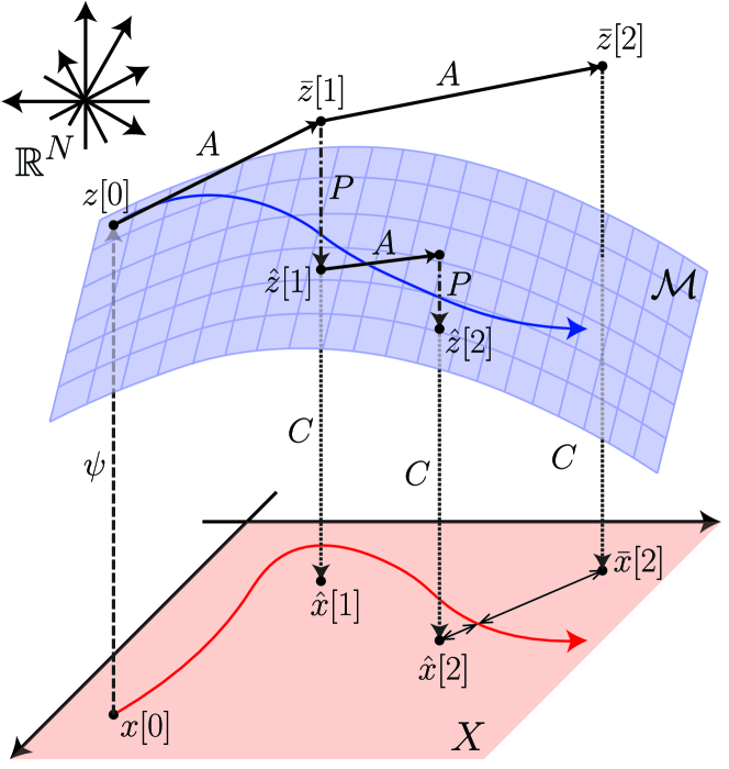
Figure 2: An illustration of the effect of deviating from the image of the lifted functions ${\cal M}$ and how it can be remedied by defining a projection operation as described in Section II-D. The evolution of the finite dimensional system in the state space $X$ from $x_{0}$ is depicted as a red curve. The lifted version of this evolution is depicted as the blue curve which is contained in $\cal{M}$. The discrete time system representation in the higher-dimensional space created by iteratively applying the state matrix $A$ to $z[j]$ may generate a solution that is outside of ${\cal M}$. Though one can still apply $C$ to $\bar{z}$ to project it back to $X$, this may result in poor performance. Instead, by projecting $\bar{z}[j]$ onto the manifold at each discrete time step to define a new lifted state $\hat{z}[j]$, the deviation from $\cal{M}$ is reduced, which improves overall predictive performance.

A pitfall of data-driven modeling approaches is the tendency to overfit. While least-squares regression yields a solution that minimizes the total $L^{2}$ error with respect to the training data, this solution can be particularly susceptible to outliers and noise [25]. To guard against overfitting to noise while identifying $\bar{U}_{T_{s}}$, we utilize the $L^{1}$-regularization method of Least Absolute Shrinkage and Selection Operator (LASSO) [31]:

$$\hat{\vec{U}}_{T_{s}} = \text{arg}~{}\underset{\vec{U}_{T_{s}}}{\text{min}} ||\vec{\Gamma}_{\alpha}\vec{U}_{T_{s}}-\vec{\Gamma}_{\beta}||_{2}^{2}+\lambda||\vec{U}_{T_{s}}||_{1}$$ (27)

where $\lambda\in\mathbb{R}^{+}$ is the weight of the $L^{1}$ penalty term, and $\vec{\cdot}$ denotes a vectorized version of each matrix with dimensions consistent with the stated problem. For $\lambda=0$, (27) provides the same unique least-squares solution as (22); as $\lambda$ increases it drives the elements of $\vec{U}_{T_{s}}$ to zero. For an overview of the LASSO method and its implementation see Tibshirani [31].

The benefit of using $L^{1}$-regularization to reduce overfitting rather than $L^{2}$-regularization (e.g. ridge regression) is its ability to drive elements to zero, rather than just making them small. This promotes sparsity in the resulting Koopman operator matrix (and consequently the $A$ and $B$ matrices). Sparsity is desirable since it reduces the memory needed to store these matrices on a computer, enabling a higher dimensional set of basis functions to be used to construct the lifting function $\psi$.

Though sparsity is desirable, it can come at the loss of accuracy in prediction. As illustrated in Fig. 2, the lifting function $\psi$ maps from $\mathbb{R}^{n}$ to $\mathcal{M}$, but at some time step $j$, $A\psi(a[j])+Bu[j]$ may not map onto $\mathcal{M}$. When this happens and we try to simulate our linear model from an initial condition, it may leave the space of legitimate “lifted states” rapidly and fail to predict behavior accurately. We therefore desire the sparsest model that minimizes the distance from $\mathcal{M}$ at each iteration.

This can be accomplished by applying a projection operator at each time step. For each snapshot pair, the ideal projection operator $P$ should satisfy the following for all $k$

$$P\left(A{\psi}(a[k])+Bu[k]\right) =\psi(b[k]).$$ (28)

To build an approximation to this operator, we construct the following $K\times N$ matrix,

$$\Omega_{a}:=\begin{bmatrix}\left(A{\psi}(a[1])+Bu[1]\right)^{\top}\\ \vdots\\ \left(A{\psi}(a[K])+Bu[K]\right)^{\top}\end{bmatrix}.$$ (29)

Then the best projection operator in the $L^{2}$-norm sense based on our data is given by

$$P:=\left(\Omega_{a}^{\dagger}\Psi_{b}\right)^{\top}.$$ (30)

Composing $P$ with the $A$ and $B$ matrices in (19) yields a modified linear model that significantly reduces the distance from $\mathcal{M}$ at each iteration,

$$z[j+1] =\hat{A}z[j]+\hat{B}u[j]$$ (31)

where $\hat{A}:=PA$ and $\hat{B}:=PB$. Algorithm 1 summarizes the proposed model construction process.

Input: $\lambda$ , $\{a[k],b[k]\}$ and ${u[k]}$ for $k=1,...,K$

Step 1: Lift data via (6)

Step 2: Combine lifted data and inputs via (20)

Step 3: Approximate Koopman operator $\bar{U}_{T_{s}}$ via (27)

Step 4: Extract model matrices $A,B$ via (25)

Step 5: Identify projection operator $P$ via (30)

Output: $\hat{A}:=PA$, $\hat{B}:=PB$

Algorithm 1 Koopman Linear System Identification

III Model Predictive Control

A system model enables the design of model-based controllers that leverage model predictions to choose suitable control inputs for a given task. In particular, model-based controllers can anticipate future events, allowing them to optimally choose control inputs over a finite time horizon. The most popular model-based control design technique is model predictive control (MPC), wherein one optimizes the control input over a finite time horizon, applies that input for a single timestep, and then optimizes again, repeatedly [24]. For linear systems, MPC consists of iteratively solving a convex quadratic program.

Importantly, this is also the case for Koopman-based MPC control, wherein one solves the following program at each time instance $k$ of the closed-loop operation:

$$\underset{u[i],z[i]}{\text{min}} z[N_{h}]^{T}G_{N_{h}}z[N_{h}]+g_{N_{h}}^{T}z[N_{h}]+$$ (32)

$$+\sum_{i=0}^{N_{h}-1}z[i]^{T}G_{i}z[i]+u[i]^{T}H_{i}u[i]+g_{i}^{T}z[i]+h_{i}^{T}u[i]$$

s.t. $$z[i+1]=\hat{A}z[i]+\hat{B}u[i],\quad\forall i\in\{0,\ldots,N_{h}-1\}$$

$$E_{i}z[i]+F_{i}u[i]\leq b_{i},\quad\forall i\in\{0,\ldots,N_{h}-1\}$$

$$z[0]=\psi(x[k])$$

where $N_{h}\in\mathbb{N}$ is the prediction horizon, $G_{i}\in\mathbb{R}^{N\times N}$ and $H_{i}\in\mathbb{R}^{m\times m}$ are positive semidefinite matrices, and where each time the program is called, the predictions are initialized from the current lifted state $\psi(x[k])$. The matrices $E_{i}\in\mathbb{R}^{c\times N}$ and $F_{i}\in\mathbb{R}^{c\times m}$ and the vector $b_{i}\in\mathbb{R}^{c}$ define state and input polyhedral constraints where $c$ denotes the number of imposed constraints. While the size of the cost and constraint matrices in (32) depend on the dimension of the lifted state $N$, Korda and Mezić [14] show these can be rendered independent of $N$ by transforming the problem into its so-called ”dense-form.” Algorithm 2 summarizes the closed-loop operation of this Koopman based MPC controller.

Input: Prediction horizon: $N_{h}$

           Cost matrices: $G_{i},H_{i},g_{i},h_{i}$ for $i=0,...,N_{h}$

           Constraint matrices: $E_{i},F_{i},b_{i}$ for $i=0,...,N_{h}$

           Model matrices: $\hat{A},\hat{B}$

for  $k=0,1,2,...$ do

       Step 1: Set $z[0]=\psi(x[k])$

       Step 2: Solve (32) to find optimal input $(u[i]^{*})_{i=0}^{N_{h}}$

       Step 3: Set $u[k]=u[0]^{*}$

       Step 4: Apply $u[k]$ to the system

end for

Algorithm 2 Koopman-Based MPC

Since this optimization problem is convex, it has a unique globally optimal solution that can efficiently be constructed without initialization [4] for models with thousands of states and inputs [21, 28]. This contrasts sharply with the MPC formulation for nonlinear systems (referred to as nonlinear model predictive control or NMPC [2]). NMPC requires solving an optimization problem with nonlinear constraints and a (potentially) nonlinear cost function. As a result, algorithms to solve such problems typically require initialization and can struggle to find globally optimal solutions [23]. Though techniques have been proposed to improve the speed of algorithms to solve NMPC problems [20, 11] or even globally solve such problems without requiring initialization [37], these formulations still take several seconds per iteration, which can make them too slow to be applied during real-time control.

IV Experiments

This section describes the robot and the set of experiments used to demonstrate the efficacy of the modeling and control methods from Sections II and III. Video of the soft robot performing several tasks from the final experiment is included in a supplementary video file.

IV-A Robot Description: Soft Arm with Laser Pointer

The robot used for the experiments is a suspended soft arm with a laser pointer attached to the end effector (see Fig. 3). The laser dot is projected onto a ${50\text{ cm}\times 50\text{ cm}}$ flat board which sits $34\text{ cm}$ beneath the tip of the laser pointer when the robot is in its relaxed position (i.e. hanging straight down). The position of the laser dot is measured by a digital webcam overlooking the board.

The arm itself consists of two sections that are each composed of three pneumatic artificial muscles or PAMs (also known as McKibben actuators [33]) adhered to a central foam spine by latex rubber bands (see Fig. 3). The PAMs in the upper and lower sections are internally connected so that only three input pressure lines are required, and they are arranged such that for any bending of the upper section, bending in the opposite direction occurs in the bottom section. This ensures that the laser pointer mounted to the end effector points approximately vertically downward so that the laser light strikes the board at all times. The pressures inside the actuators are regulated by three Enfield TR-010-g10-s pneumatic pressure regulators, which accept ${0-10}$V command signals corresponding to pressures of ${\approx 0-140}$ kPa. In the experiments there is a three-dimensional input corresponding to the voltages into the three pressure regulators and a two dimensional state corresponding to the position of the laser dot with respect to the center of the board.

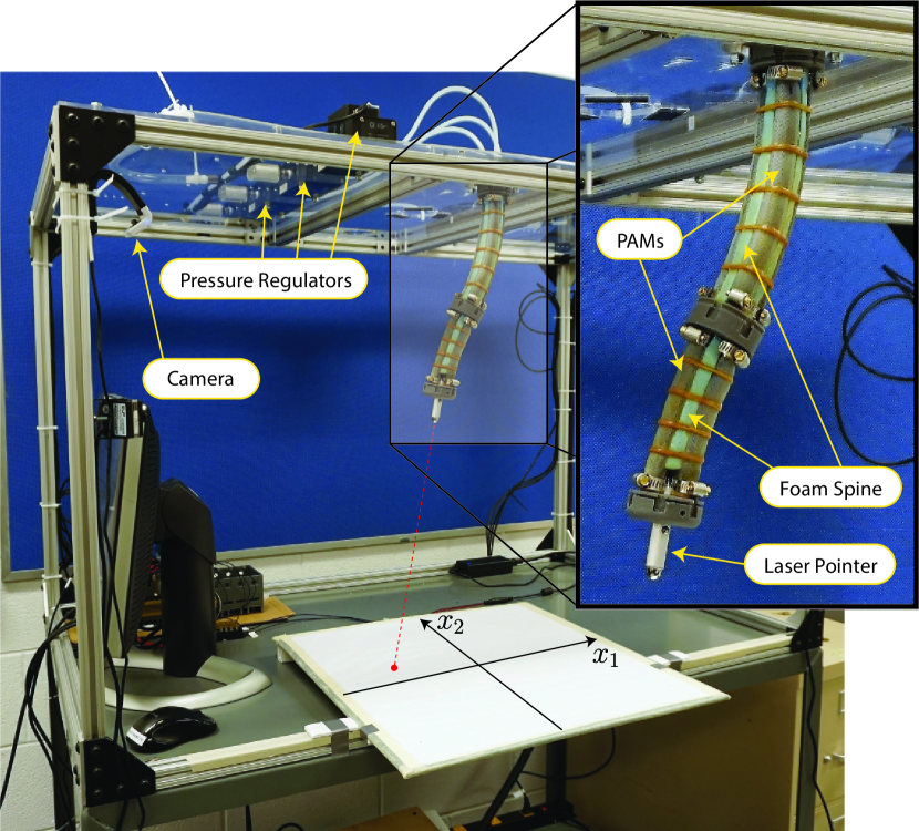
Figure 3: The soft robot consists of two bending segments with a laser pointer attached to the end effector. A set of three pressure regulators is used to control the pressure inside of the pneumatic actuators (PAMs), and a camera is used to track the position of the laser dot.

IV-B Characterization of Stochastic Behavior

Most mechanical systems demonstrate stochastic behavior (i.e. when an identical input and state produces a different output) to some extent. Stochastic behavior is characteristic of electronic pressure regulators, which can limit the precision of pneumatically driven soft robotic systems and undermine the predictive capability of models.

We quantified the stochastic behavior of our soft robot system by observing the variations in output from period-to-period under sinusoidal inputs to the three actuators of the form

$$u[k] =\begin{bmatrix}6\sin(\frac{2\pi}{T}kT_{s})+3\vspace{5pt}\\ 6\sin(\frac{2\pi}{T}kT_{s}-\frac{T}{3})+3\vspace{5pt}\\ 6\sin(\frac{2\pi}{T}kT_{s}-\frac{2T}{3})+3\end{bmatrix}$$ (33)

for periods of $T=6,7,8,9,10,11,12$ seconds and a sampling time of $T_{s}=0.1$ seconds with a zero-order-hold between samples. Under these inputs, the laser dot traces out a circle with some variability in the trajectory over each period. In Fig. 4 the trajectories over 210 periods are superimposed along with the average over all trials. Nearly all of the observed points fell within 1 cm of the mean trajectory. Given this inherent stochasticity of our soft robotic system, in the best case we expect only to be able to control the output to within $\approx 1$ cm of a desired trajectory.

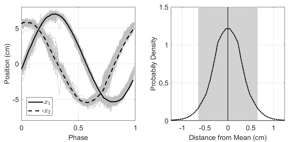
Figure 4: The left plot shows the average response of the system over a single period when the sinusoidal inputs of varying frequencies described by (33) are applied. All of the particular responses are subimposed in light grey. The right plot shows the distribution of trajectories about the mean, with all distances within two standard deviations highlighted in grey. The width of the distribution illustrates how for the soft robot system identical inputs can produce outputs that vary by up to 2 cm.

IV-C Data Collection and Model Identification

To construct a model, we ran the system through $16$ trials each lasting approximately $20$ minutes. A randomized input was applied during each trial to generate a representative sampling of the system’s behavior over its entire operating range. To ensure randomization, a matrix $\Upsilon\in[0,10]^{3\times 1000}$ of uniformly distributed random numbers between zero and ten was generated to be used as an input lookup table. Each control input was smoothly varied between elements in consecutive columns of the table over a transition period $T_{u}$, with a time offset of $T_{u}/3$ between each of the three control signals

$$u_{i}(t) =\frac{(\Upsilon_{i,k+1}-\Upsilon_{i,k})}{T_{u}}\left(t+\frac{(i-1)T_{u}}{3}\right)+\Upsilon_{i,k}$$ (34)

where $k=\text{floor}\left({t}/{T_{u}}\right)$ is the current index into the lookup table at time $t$. The transition period $T_{u}$ varied from $5$ seconds to $10$ seconds between trials. After collection, the data was uniformly sampled with period $T_{s}=0.1$ seconds.

Two models were fit from the data: a Koopman model, and a linear state space model. The linear state-space model provides a baseline for comparison and was identified from the same data as the Koopman model using the MATLAB System Identification Toolbox [17]. This model is a four dimensional linear state-space model expressed in observer canonical form. The Koopman model was identified via the method described in Section II on a set of $191,000$ snapshot pairs $\{a[k],b[k]\}$ that incorporate a single delay $d=1$:

$$a[k] =\begin{bmatrix}x[k]^{\top}&x[k-1]^{\top}&u[k-1]^{\top}\end{bmatrix}^{\top}$$ (35)

$$b[k] =\begin{bmatrix}\left(\phi_{T_{s}}(x[k])+\sigma[k]\right)^{\top}&x[k]^{\top}&u[k]^{\top}\end{bmatrix}^{\top},$$ (36)

and using an $N=330$ dimensional set of basis functions consisting of all monomials of maximum degree 4. To find the sparsest acceptable matrix representation of the Koopman operator, equation (27) was solved for ${\lambda=0,1,2,...,50}$. Predictions from the resulting models were evaluated against a subset of the training data, with the error quantified as the average Euclidean distance between the prediction and actual trajectory at each point, normalized by dividing by the average Euclidean distance between the actual trajectory and the origin. Fig. 5 shows that as $\lambda$ increases so does this error, but the density of the $\hat{A}$ matrix of the lifted linear model decreases. The model chosen is the one that minimizes prediction error, which results in an $\hat{A}$ matrix with $70\%$ of its entries equal to zero.

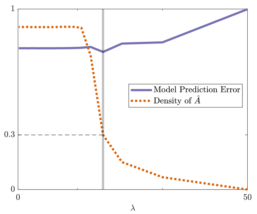
Figure 5: As $\lambda$ (the weight of the $L^{1}$ penalty term in (27)) increases, the density of the lifted system matrix $\hat{A}$ decreases. The model generated by solving (27) with the value of $\lambda$ designated by the vertical grey bar has lower error and a sparser $\hat{A}$ matrix than the least-squares solution to (22), which occurs at $\lambda=0$.

IV-D Experiment 1: Model Prediction Comparison

The accuracy of the predictions generated by each of the two models were evaluated by comparing them to the actual behavior of the system under the sinusoidal inputs defined in (33). The model responses were simulated over a time horizon of $2.5$ seconds given the same initial condition and input as the real system. The results of this comparison are summarized by Fig. 6 and Table I. They illustrate that the Koopman model predictions are more accurate over the time horizon.

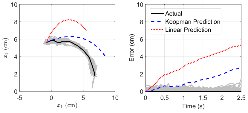
Figure 6: The (average) actual response and the model predictions for the robot over a 2.5 second horizon with the sinusoidal inputs described in (33) with period $T=10$ seconds applied. The left plot shows the actual trajectory of the laser dot along with model predictions. The error displayed on the right plot is defined as the Euclidean distance between the predicted laser dot position and the actual position at each point in time. The prediction error is smaller for the Koopman model over the entire horizon.

TABLE I: Average Prediction Error Over 2.5 second Horizon (cm)

	Period of Sinusoidal Inputs (seconds)
Model	6	7	8	9	10	11	12	Avg.
Koopman	2.21	2.78	1.35	1.53	1.21	0.66	1.41	1.59
Linear S.S.	4.64	4.54	3.94	3.56	3.15	2.72	2.83	3.63

IV-E Experiment 2: Model-Based Control Comparison

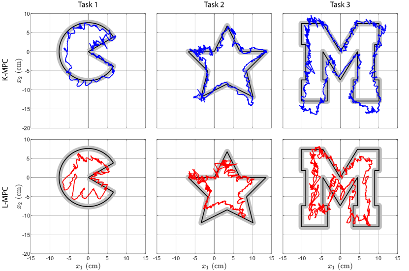
Figure 7: The results of the K-MPC controller (row 1, blue) and the L-MPC controller (row 2, red) in performing trajectory following tasks 1-3. The reference trajectory for each task is subimposed in black as well as a grey buffer with width equal to two standard deviations of the noise probability density shown in Fig. 4.

The two identified models were each used to build a model predictive controller which solves an optimization problem in the form of (32) at each time step using the Gurobi Optimization software [10]. We refer to the two controllers by the abbreviations K-MPC for the one based on the Koopman model, and L-MPC for the one based on the linear state-space model. Both model predictive controllers run in closed-loop at $10$ Hz, feature an MPC horizon of 2.5 seconds ($N_{h}=25$), and a cost function that penalizes deviations from a reference trajectory $r[k]$ over the horizon with both a running and terminal cost:

Cost $$=100\left(y[N_{h}]-r[N_{h}]\right)^{2}+\sum_{i=0}^{N_{h}-1}0.1\left(y[i]-r[i]\right)^{2}$$ (37)

In the K-MPC case, $y[i]=Cz[i]$, where $C$ is defined as in (26). In the L-MPC case, $y[i]=C_{L}x_{L}[i]$ where $x_{L}$ is the four dimensional system state and $C_{L}$ is the projection matrix that isolates the states describing the current laser dot coordinates.

The performance of the controllers was assessed with respect to a set of three trajectory following tasks. Each task was to follow a reference trajectory as it traced out one of the following shapes over a certain amount of time:

1. Pacman (90 seconds)

2. Star (180 seconds)

3. Block letter M (300 seconds)

The error for each trial was quantified as the Euclidean distance from the reference trajectory at each time step over the length of the trial.

The performances of the K-MPC and L-MPC controllers at Tasks 1, 2, and 3 are shown visually in Fig. 7, and the error is quantified in Table II. In both tasks the K-MPC controller achieved better performance, exhibiting an average tracking error of 1.26 cm compared to the L-MPC controller’s average error of 2.45 cm. This amounts to an average error roughly $25\%$ larger than than the maximum magnitude of observed noise (see Fig. 4)

TABLE II: Average Error in Trajectory Following Tasks (cm)

	Task				Std.
Controller	$1$	$2$	$3$	Avg.	Dev.
K-MPC	1.25	1.19	1.34	1.26	0.07
L-MPC	2.21	2.34	2.73	2.45	0.31

V Conclusion

In this work, a data-driven modeling and control method based on Koopman operator theory was successfully applied to a soft robot. The Koopman-based MPC controller was shown to be capable of commanding a soft robot to follow a reference trajectory better than an MPC controller based on another linear data-driven model. By making explicit control-oriented models of soft robots easier to construct, this method enables the rapid development of new control strategies and applications.

While these preliminary results are promising, further work is needed to make such methods feasible for higher dimensional robotic systems. Toward that end, this work introduced a method for promoting sparsity in matrix representations of the Koopman model. Additional work will explore strategies for further promoting sparsity, choosing the most effective basis of observables, and building models that can account for external loading and contact forces.

References

- Abraham et al. [2017] Ian Abraham, Gerardo de la Torre, and Todd Murphey. Model-based control using koopman operators. In Proceedings of Robotics: Science and Systems, Cambridge, Massachusetts, July 2017. doi: 10.15607/RSS.2017.XIII.052.
- Allgöwer and Zheng [2012] Frank Allgöwer and Alex Zheng. Nonlinear model predictive control, volume 26. Birkhäuser, 2012.
- Ansari and Murphey [2016] Alexander R Ansari and Todd D Murphey. Sequential action control: Closed-form optimal control for nonlinear and nonsmooth systems. IEEE Trans. Robotics, 32(5):1196–1214, 2016.
- Boyd and Vandenberghe [2004] Stephen Boyd and Lieven Vandenberghe. Convex optimization. Cambridge university press, 2004.
- Bruder et al. [2018a] D. Bruder, A. Sedal, R. Vasudevan, and C. D. Remy. Force generation by parallel combinations of fiber-reinforced fluid-driven actuators. IEEE Robotics and Automation Letters, 3(4):3999–4006, Oct 2018a. ISSN 2377-3766. doi: 10.1109/LRA.2018.2859441.
- Bruder et al. [2018b] Daniel Bruder, C David Remy, and Ram Vasudevan. Nonlinear system identification of soft robot dynamics using koopman operator theory. arXiv preprint arXiv:1810.06637, 2018b.
- Budišić et al. [2012] Marko Budišić, Ryan Mohr, and Igor Mezić. Applied koopmanism. Chaos: An Interdisciplinary Journal of Nonlinear Science, 22(4):047510, 2012.
- Gillespie et al. [2018] Morgan T Gillespie, Charles M Best, Eric C Townsend, David Wingate, and Marc D Killpack. Learning nonlinear dynamic models of soft robots for model predictive control with neural networks. In 2018 IEEE International Conference on Soft Robotics (RoboSoft). IEEE, 2018.
- Gravagne et al. [2003] Ian A Gravagne, Christopher D Rahn, and Ian D Walker. Large deflection dynamics and control for planar continuum robots. IEEE/ASME transactions on mechatronics, 8(2):299–307, 2003.
- Gurobi Optimization [2018] LLC Gurobi Optimization. Gurobi optimizer reference manual, 2018. URL http://www.gurobi.com.
- Hereid and Ames [2017] Ayonga Hereid and Aaron D Ames. Frost∗: Fast robot optimization and simulation toolkit. In Intelligent Robots and Systems (IROS), 2017 IEEE/RSJ International Conference on, pages 719–726. IEEE, 2017.
- Howell et al. [1996] Larry L Howell, Ashok Midha, and TW Norton. Evaluation of equivalent spring stiffness for use in a pseudo-rigid-body model of large-deflection compliant mechanisms. Journal of Mechanical Design, 118(1):126–131, 1996.
- Ilievski et al. [2011] Filip Ilievski, Aaron D Mazzeo, Robert F Shepherd, Xin Chen, and George M Whitesides. Soft robotics for chemists. Angewandte Chemie, 123(8):1930–1935, 2011.
- Korda and Mezić [2018] Milan Korda and Igor Mezić. Linear predictors for nonlinear dynamical systems: Koopman operator meets model predictive control. Automatica, 93:149–160, 2018.
- Lasota and Mackey [2013] Andrzej Lasota and Michael C Mackey. Chaos, fractals, and noise: stochastic aspects of dynamics, volume 97. Springer Science & Business Media, 2013.
- Marchese et al. [2014] Andrew D Marchese, Cagdas D Onal, and Daniela Rus. Autonomous soft robotic fish capable of escape maneuvers using fluidic elastomer actuators. Soft Robotics, 1(1):75–87, 2014.
- MATLAB [2017] MATLAB. version 7.10.0 (R2017a). The MathWorks Inc., Natick, Massachusetts, 2017.
- Mauroy and Goncalves [2016] Alexandre Mauroy and Jorge Goncalves. Linear identification of nonlinear systems: A lifting technique based on the koopman operator. arXiv preprint arXiv:1605.04457, 2016.
- Mauroy and Goncalves [2017] Alexandre Mauroy and Jorge Goncalves. Koopman-based lifting techniques for nonlinear systems identification. arXiv preprint arXiv:1709.02003, 2017.
- Patterson and Rao [2014] Michael A Patterson and Anil V Rao. Gpops-ii: A matlab software for solving multiple-phase optimal control problems using hp-adaptive gaussian quadrature collocation methods and sparse nonlinear programming. ACM Transactions on Mathematical Software (TOMS), 41(1):1, 2014.
- Paulson et al. [2014] Joel A Paulson, Ali Mesbah, Stefan Streif, Rolf Findeisen, and Richard D Braatz. Fast stochastic model predictive control of high-dimensional systems. In Decision and Control (CDC), 2014 IEEE 53rd Annual Conference on, pages 2802–2809. IEEE, 2014.
- Penrose [1956] Roger Penrose. On best approximate solutions of linear matrix equations. In Mathematical Proceedings of the Cambridge Philosophical Society, volume 52, pages 17–19. Cambridge University Press, 1956.
- Polak [2012] Elijah Polak. Optimization: algorithms and consistent approximations, volume 124. Springer Science & Business Media, 2012.
- Rawlings and Mayne [2009] James B Rawlings and David Q Mayne. Model predictive control: Theory and design. Nob Hill Pub. Madison, Wisconsin, 2009.
- Rousseeuw and Leroy [2005] Peter J Rousseeuw and Annick M Leroy. Robust regression and outlier detection, volume 589. John wiley & sons, 2005.
- Rus and Tolley [2015] Daniela Rus and Michael T Tolley. Design, fabrication and control of soft robots. Nature, 521(7553):467, 2015.
- Spong and Vidyasagar [2008] M.W. Spong and M. Vidyasagar. Robot Dynamics And Control. Wiley India Pvt. Limited, 2008. ISBN 9788126517800. URL https://books.google.com/books?id=PtxYAv7ZUYMC.
- Stellato et al. [2018] Bartolomeo Stellato, Goran Banjac, Paul Goulart, Alberto Bemporad, and Stephen Boyd. Osqp: An operator splitting solver for quadratic programs. In 2018 UKACC 12th International Conference on Control (CONTROL), pages 339–339. IEEE, 2018.
- Tedrake et al. [2010] Russ Tedrake, Ian R Manchester, Mark Tobenkin, and John W Roberts. Lqr-trees: Feedback motion planning via sums-of-squares verification. The International Journal of Robotics Research, 29(8):1038–1052, 2010.
- Thuruthel et al. [2018] Thomas George Thuruthel, Egidio Falotico, Federico Renda, and Cecilia Laschi. Model-based reinforcement learning for closed-loop dynamic control of soft robotic manipulators. IEEE Transactions on Robotics, 2018.
- Tibshirani [1996] Robert Tibshirani. Regression shrinkage and selection via the lasso. Journal of the Royal Statistical Society. Series B (Methodological), pages 267–288, 1996.
- Tolley et al. [2014] Michael T Tolley, Robert F Shepherd, Bobak Mosadegh, Kevin C Galloway, Michael Wehner, Michael Karpelson, Robert J Wood, and George M Whitesides. A resilient, untethered soft robot. Soft robotics, 1(3):213–223, 2014.
- Tondu [2012] Bertrand Tondu. Modelling of the mckibben artificial muscle: A review. Journal of Intelligent Material Systems and Structures, 23(3):225–253, 2012.
- Trivedi et al. [2008] Deepak Trivedi, Amir Lotfi, and Christopher D Rahn. Geometrically exact models for soft robotic manipulators. IEEE Transactions on Robotics, 24(4):773–780, 2008.
- Webster III and Jones [2010] Robert J Webster III and Bryan A Jones. Design and kinematic modeling of constant curvature continuum robots: A review. The International Journal of Robotics Research, 29(13):1661–1683, 2010.
- Williams et al. [2015] Matthew O Williams, Ioannis G Kevrekidis, and Clarence W Rowley. A data–driven approximation of the koopman operator: Extending dynamic mode decomposition. Journal of Nonlinear Science, 25(6):1307–1346, 2015.
- Zhao et al. [2017] Pengcheng Zhao, Shankar Mohan, and Ram Vasudevan. Control synthesis for nonlinear optimal control via convex relaxations. In American Control Conference (ACC), 2017, pages 2654–2661. IEEE, 2017.