arXiv:yymm.nnnn

Stability of the vacuum as constraint on $U$(1) extensions of the standard model

Zoltán Péli^a and Zoltán Trócsányi^a,b,

^aMTA-DE Particle Physics Research Group,
H-4010 Debrecen, PO Box 105, Hungary
^bInstitute for Theoretical Physics, Eötvös Loránd University,
Pázmány Péter sétány 1/A, H-1117 Budapest, Hungary
E-mail: Zoltan.Trocsanyi@cern.ch

Abstract

In the standard model the running quartic coupling becomes negative during its renormalization group flow, which destabilizes the vacuum. We consider U(1) extensions of the standard model, with an extra complex scalar field and a Majorana-type neutrino Yukawa coupling. These additional couplings affect the renormalization group flow of the quartic couplings. We compute the beta-functions of the extended model at one-loop order in perturbation theory and study how the parameter space of the new scalar couplings can be constrained by the requirement of stable vacuum and perturbativity up to the Planck scale.

2019

The standard model of elementary particle interactions [1] has been proven experimentally to high precision at the Large Electron Positrion Collider [2] and also at the Large Hadron Collider (LHC) [3, 4]. At the LHC the last missing piece, the Higgs particle has also been discovered and its mass has been measured at high precision [5, 6], which made possible the precise renormalization group (RG) flow analysis of the Brout-Englert-Higgs potential [7, 8]. The perturbative precision of this computation is sufficiently high so that the conclusion about the instability of the vacuum in the standard model cannot be questioned. While the instability may not influence the fate of our present Universe if the tunneling rate from the false vacuum is sufficiently low (making the Universe metastable), one may insist that the vacuum must be stable up to the Planck scale. Indeed, if we assume the natural proposition that cosmological time is inversely proportional to the relevant energy scale of particle processes, then short after the Big Bang the Universe based on the standard model were unstable and could not exist, which calls for an extension of the standard model.

In this letter we consider the simplest possible extension of the standard model gauge group $G_{\mathrm{SM}}=SU(3)_{\mathrm{c}}\otimes SU(2)_{\mathrm{L}}\otimes U(1)_{Y}$ to $G_{\mathrm{SM}}\otimes U(1)_{Z}$ and study the renormalization group flow of the scalar couplings at one-loop order in perturbation theory. Although, we are motivated by a specific model of such extensions [9], for small values of the new gauge couplings–as suggested by other phenomenological considerations–the only relevant couplings are the scalar ones and the largest Yukawa-coupling in the neutrino sector if we assume similar hierarchy of the latter as one can observe for u-type quarks in the standard model [10]. Hence, the precise formulation of the gauge sector does not influence our conclusions and we need to focus on the formulation of the scalar sector.

Our scalar sector is defined similarly as in the standard model, but in addition to the usual scalar field $\phi$ that is an $SU(2)_{\mathrm{L}}$-doublet

$$\phi=\left(\!\!\begin{array}[]{c}\phi^{+}\\ \phi^{0}\end{array}\!\!\right)=\frac{1}{\sqrt{2}}\left(\!\!\begin{array}[]{c}\phi_{1}+\mathrm{i}\phi_{2}\\ \phi_{3}+\mathrm{i}\phi_{4}\end{array}\!\!\right)\,,$$ (1)

there is also another complex scalar $\chi$ that transforms as a singlet under $G_{\rm SM}$ transformations. The gauge invariant Lagrangian of the scalar fields is

$$\mathcal{L}_{\phi,\chi}=[D^{(\phi)}_{\mu}\phi]^{*}D^{(\phi)\,\mu}\phi+[D^{(\chi)}_{\mu}\chi]^{*}D^{(\chi)\,\mu}\chi-V(\phi,\chi)\,.$$ (2)

The covariant derivative for the scalar $s$ ($s=\phi$, $\chi$) is

$$D_{\mu}^{\left(s\right)}=\partial_{\mu}+\mathrm{i}g_{\mathrm{L}}\,{\mbox{\boldmath$T$}}\cdot{\mbox{\boldmath$W$}}_{\mu}+\mathrm{i}\,y_{s}g_{Y}B^{\prime}_{\mu}+\mathrm{i}\left(r_{s}g^{\prime}_{Z}+y_{s}g^{\prime}_{ZY}\right)Z^{\prime}_{\mu}$$ (3)

where ${\mbox{\boldmath$T$}}=(T^{1},T^{2},T^{3})$ are the generators and $g_{\mathrm{L}}$ is the coupling of the $SU(2)_{\mathrm{L}}$ group, $g_{Y}$ is the $U(1)_{Y}$ coupling, $g^{\prime}_{Z}=g_{Z}/\cos\theta_{Z}$ is the ratio of the $U(1)_{Z}$ coupling and the cosine of the kinetic mixing angle and $g^{\prime}_{ZY}=g^{\prime}_{Z}-g_{Y}\tan\theta_{Z}$ is the mixed coupling [11], while $y_{s}$, $r_{s}$ are the corresponding hyper- and super-weak charges of the scalars. In the renormalization group analysis below we shall concentrate on the phenomenologically relevant case when the new couplings are super-weak, hence negligible in the scalar sector, and so the actual values of $r_{s}$ are irrelevant.

In Eq. (2) the potential energy

$$V(\phi,\chi)=V_{0}-\mu_{\phi}^{2}|\phi|^{2}-\mu_{\chi}^{2}|\chi|^{2}+\left(|\phi|^{2},|\chi|^{2}\right)\left(\!\!\begin{array}[]{cc}\lambda_{\phi}&\frac{\lambda}{2}\\ \frac{\lambda}{2}&\lambda_{\chi}\end{array}\!\!\right)\left(\!\!\begin{array}[]{c}|\phi|^{2}\\ |\chi|^{2}\end{array}\!\!\right)\,,$$ (4)

in addition to the usual quartic terms, introduces a coupling term $-\lambda|\phi|^{2}|\chi|^{2}$ of the scalar fields in the Lagrangian where $|\phi|^{2}=|\phi^{+}|^{2}+|\phi^{0}|^{2}$. The value of the additive constant $V_{0}$ is irrelevant for particle dynamics, but may be relevant for inflationary scenarios, hence we allow a non-vanishing value for it. In order that this potential energy be bounded from below, we have to require the positivity of the self-couplings, $\lambda_{\phi}$, $\lambda_{\chi}>0$. The eigenvalues of the coupling matrix are

$$\lambda_{\pm}=\frac{1}{2}\left(\lambda_{\phi}+\lambda_{\chi}\pm\sqrt{(\lambda_{\phi}-\lambda_{\chi})^{2}+\lambda^{2}}\right)\,,$$ (5)

with $\lambda_{+}>0$ and $\lambda_{-}<\lambda_{+}$. In the physical region the potential can be unbounded from below only if $\lambda_{-}<0$ and the eigenvector belonging to $\lambda_{-}$ points into the first quadrant, which may occur only when $\lambda<0$. In this case, the potential will be bounded from below if the coupling matrix is positive definite, i.e.

$$4\lambda_{\phi}\lambda_{\chi}-\lambda^{2}>0\,.$$ (6)

If these conditions are satisfied, we find the minimum of the potential energy at field values $\phi=v/\sqrt{2}$ and $\chi=w/\sqrt{2}$ where the vacuum expectation values (VEVs) are

$$v=\sqrt{2}\sqrt{\frac{2\lambda_{\chi}\mu_{\phi}^{2}-\lambda\mu_{\chi}^{2}}{4\lambda_{\phi}\lambda_{\chi}-\lambda^{2}}}\,,\qquad w=\sqrt{2}\sqrt{\frac{2\lambda_{\phi}\mu_{\chi}^{2}-\lambda\mu_{\phi}^{2}}{4\lambda_{\phi}\lambda_{\chi}-\lambda^{2}}}\,.$$ (7)

Using the VEVs, we can express the quadratic couplings as

$$\mu_{\phi}^{2}=\lambda_{\phi}v^{2}+\frac{\lambda}{2}w^{2}\,,\qquad\mu_{\chi}^{2}=\lambda_{\chi}w^{2}+\frac{\lambda}{2}v^{2}\,,$$ (8)

so those are both positive if $\lambda>0$. If $\lambda<0$, the constraint (6) ensures that the denominators of the VEVs in Eq. (7) are positive, so the VEVs have non-vanishing real values only if

$$2\lambda_{\chi}\mu_{\phi}^{2}-\lambda\mu_{\chi}^{2}>0\quad\text{and}\quad 2\lambda_{\phi}\mu_{\chi}^{2}-\lambda\mu_{\phi}^{2}>0$$ (9)

simultaneously, which can be satisfied if at most one of the quadratic couplings is smaller than zero. We summarize the possible cases for the signs of the couplings in Table 1.

Table 1: Possible signs of the couplings in the scalar potential $V(\phi,\chi)$ in order to have two non-vanishing real VEVs. $\Theta$ is the step function, $\Theta(x)=1$ if $x>0$ and 0 if $x<0$

$\Theta(\lambda)$	$\Theta(\lambda_{\phi})$	$\Theta(\lambda_{\chi})$	$\Theta(4\lambda_{\phi}\lambda_{\chi}-\lambda^{2})$	$\Theta(\mu_{\phi}^{2})\,\Theta(\mu_{\chi}^{2})$	$\Theta(2\lambda_{\chi}\mu_{\phi}^{2}-\lambda\mu_{\chi}^{2})\Theta(2\lambda_{\phi}\mu_{\chi}^{2}-\lambda\mu_{\phi}^{2})$
1	1	1	unconstrained	1	unconstrained
0	1	1	1	1	unconstrained
0	1	1	1	0	1

After spontaneous symmetry breaking of $G\to SU(3)_{\mathrm{c}}\otimes U(1)_{Q}$ we use the following convenient parametrization for the scalar fields:

$$\phi=\frac{1}{\sqrt{2}}\,\mathrm{e}^{\mathrm{i}{\mbox{\boldmath$T$}}\cdot{\mbox{\boldmath$\xi$}}(x)/v}\left(\!\!\begin{array}[]{c}0\\ v+h^{\prime}(x)\end{array}\!\!\right)\quad\mbox{and}\quad\chi(x)=\frac{1}{\sqrt{2}}\,\mathrm{e}^{\mathrm{i}\eta(x)/w}\big{(}w+s^{\prime}(x)\big{)}\,.$$ (10)

We can use the gauge invariance of the model to choose the unitary gauge when

$$\phi^{\prime}(x)=\frac{1}{\sqrt{2}}\left(\!\!\begin{array}[]{c}0\\ v+h^{\prime}(x)\end{array}\!\!\right)\quad\mbox{and}\quad\chi^{\prime}(x)=\frac{1}{\sqrt{2}}\big{(}w+s^{\prime}(x)\big{)}\,.$$ (11)

With this gauge choice, the scalar kinetic term contains quadratic terms of the gauge fields from which one can identify mass parameters of the massive standard model gauge bosons proportional to the vacuum expectation value $v$ of the BEH field and also that of a massive vector boson $Z^{{}^{\prime}\mu}$ proportional to $w$.

We can diagonalize the mass matrix (quadratic terms) of the two real scalars ($h^{\prime}$ and $s^{\prime}$) by the rotation

$$\left(\!\!\begin{array}[]{c}h\\ s\end{array}\!\!\right)=\left(\!\!\begin{array}[]{cr}\cos\theta_{S}&-\sin\theta_{S}\\ \sin\theta_{S}&\cos\theta_{S}\end{array}\!\!\right)\left(\!\!\begin{array}[]{c}h^{\prime}\\ s^{\prime}\end{array}\!\!\right)$$ (12)

where for the scalar mixing angle $\theta_{S}\in(-\frac{\pi}{4},\frac{\pi}{4})$ we find

$$\sin(2\theta_{S})=-\frac{\lambda vw}{\sqrt{(\lambda_{\phi}v^{2}-\lambda_{\chi}w^{2})^{2}+(\lambda vw)^{2}}}\,.$$ (13)

The masses of the mass eigenstates $h$ and $s$ are

$$M_{h/H}=\left(\lambda_{\phi}v^{2}+\lambda_{\chi}w^{2}\mp\sqrt{(\lambda_{\phi}v^{2}-\lambda_{\chi}w^{2})^{2}+(\lambda vw)^{2}}\right)^{1/2}$$ (14)

where $M_{h}\leq M_{H}$ by convention. At this point either $h$ or $H$ can be the standard model Higgs boson.

As $M_{h}$ must be positive, the condition

$$v^{2}w^{2}\Big{(}4\lambda_{\phi}\lambda_{\chi}-\lambda^{2}\Big{)}>0$$ (15)

has to be fulfilled. If both VEVs are greater than zero–as needed for two non-vanishing scalar masses–, then this condition reduces to the positivity constraint (6), but with different meaning. Eq. (6) is required to ensure that the potential be bounded from below if $\lambda<0$, which has to be fulfilled at any scale. For $\lambda>0$, the potential is bounded from below even without requiring the constraint (6). The inequality in (15) ensures $M_{h}>0$, which has to be fulfilled as long as $vw>0$ independently of the sign of $\lambda$.

The VEV of the BEH field and the mass of the Higgs boson are known experimentally, $v\simeq 262$ GeV and $m_{H}\simeq 131.55$ GeV [8]. Introducing the abbreviation $\lambda_{\mathrm{SM}}=\frac{1}{2}m_{H}^{2}/v^{2}$, we have $\lambda_{\mathrm{SM}}(m_{\mathrm{t}})\simeq 0.126$ and we can distinguish two cases at the weak scale: (i) $\lambda_{\phi}(m_{\mathrm{t}})>\lambda_{\mathrm{SM}}(m_{\mathrm{t}})$ and (ii) $\lambda_{\mathrm{SM}}(m_{\mathrm{t}})>\lambda_{\phi}(m_{\mathrm{t}})$. Then we can relate the new VEV $w$ to the BEH VEV $v$ and the four couplings $\lambda_{\mathrm{SM}}$, $\lambda_{\phi}$, $\lambda_{\chi}$, $\lambda$ using Eq. (14) as

$$w(m_{\mathrm{t}})^{2}(4(\lambda_{\phi}(m_{\mathrm{t}})-\lambda_{\mathrm{SM}}(m_{\mathrm{t}}))\lambda_{\chi}(m_{\mathrm{t}})-\lambda(m_{\mathrm{t}})^{2})=4v(m_{\mathrm{t}})^{2}\lambda_{\mathrm{SM}}(m_{\mathrm{t}})(\lambda_{\phi}(m_{\mathrm{t}})-\lambda_{\mathrm{SM}}(m_{\mathrm{t}}))\,.$$ (16)

Using Eq. (16), it is convenient to consider $w$ as a dependent parameter and scan the parameter space of the remaining three quartic couplings as done below. We are not interested in the case of $\lambda_{\phi}(m_{\mathrm{t}})=\lambda_{\mathrm{SM}}(m_{\mathrm{t}})$ because that prevents the model from interpreting neutrino masses [9].

In case (i) when $\lambda_{\phi}(m_{\mathrm{t}})>\lambda_{\mathrm{SM}}(m_{\mathrm{t}})$, then $M_{H}>m_{H}$, so only $h$ can be the Higgs particle and

$$M_{h}=m_{H}\,,\quad\textrm{while}\quad M_{H}=m_{H}\sqrt{\frac{\lambda_{\phi}-\lambda_{\mathrm{SM}}}{\lambda_{\mathrm{SM}}}}\sqrt{\frac{4\lambda_{\phi}\lambda_{\chi}-\lambda^{2}}{4(\lambda_{\phi}-\lambda_{\mathrm{SM}})\lambda_{\chi}-\lambda^{2}}}\,.$$ (17)

The positivity of $M_{H}^{2}$, in addition to the constraint in (15), also requires that

$$4(\lambda_{\phi}-\lambda_{\mathrm{SM}})\lambda_{\chi}-\lambda^{2}>0\quad\textrm{or}\quad\lambda_{\phi}>\lambda_{\mathrm{SM}}+\frac{\lambda^{2}}{4\lambda_{\chi}}\,.$$ (18)

In case (ii), $m_{H}^{2}>2\lambda_{\phi}v^{2}>M_{h}^{2}$, so only $H$ can be the Higgs particle and we can express the masses of the scalars as in Eq. (17), with $h$ and $H$ interchanged, or explicitly

$$M_{h}=m_{H}\sqrt{\frac{\lambda_{\mathrm{SM}}-\lambda_{\phi}}{\lambda_{\mathrm{SM}}}}\sqrt{\frac{4\lambda_{\phi}\lambda_{\chi}-\lambda^{2}}{\lambda^{2}+4(\lambda_{\mathrm{SM}}-\lambda_{\phi})\lambda_{\chi}}}\quad\textrm{and}\quad M_{H}=m_{H}\,,$$ (19)

which does not require any further constraint to (15).

In principle, it may happen that one of the VEVs vanishes at some critical scale $t_{c}$. In that case, for $t>t_{c}$ the only scalar particle is the Higgs boson. Thus, beyond $t_{c}$ we do not need to assume the validity of the extra constraints beyond the requirements of stability and the new scalar sector affects only the RG equations.

Neutrino oscillation experiments prove that neutrinos have masses, which in a usual gauge field theoretical description necessitates the assumption that right handed neutrinos exist. The existence of the new scalar allows for gauge invariant Majorana-type Yukawa terms of dimension four operators for the neutrinos

$$\mathcal{L}^{\nu}_{{\mathrm{Y}}}=-\frac{1}{2}\sum_{i,j}\overline{\nu_{i,{\mathrm{R}}}^{c}}\,(c_{\mathrm{R}})_{ij}\,\nu_{j,{\mathrm{R}}}\,\chi+{\rm h.c.}$$ (20)

provided the superscript $c$ denotes the charge conjugate of the field. The Yukawa coupling matrix $(c_{\mathrm{R}})_{ij}$ is a real symmetric matrix whose values are not constrained. There are other gauge invariant Yukawa terms involving the left-handed neutrinos (see Ref. [9] where all possible terms are taken into account for neutrino mass generation), but those must contain small Yukawa couplings, otherwise the left-handed neutrino masses would violate experimental constraints. In our analysis below we assume that at least one element of the diagonal matrix $O\,c_{\mathrm{R}}\,O^{T}$, with $O$ being a suitable orthogonal matrix, can take any value in the range $(0,1)$. We denote this element by $c_{\nu}$ below.

The values of the couplings at any scale are determined by the RG equations,

$$\frac{\mathrm{d}g}{\mathrm{d}t}=a\beta(g)$$ (21)

where the factor $a=\ln 10$ ensures, that the RG-time $t=\ln(\mu/{\mathrm{GeV}})$ represents the energy scale $\mu=10^{t}$ GeV rather than $\mu=e^{t}$ GeV and the variable $g$ is a generic notation for the five gauge couplings, the four most relevant Yukawa couplings $c_{\mathrm{t}}$, $c_{\mathrm{b}}$, $c_{\tau}$ and $c_{\nu}$, the two quadratic and three quartic scalar couplings (14 equations in total). In order to solve this coupled system of differential equations, we need to specify the $\beta$-functions and the initial conditions for the couplings.

At one-loop in perturbation theory, the $\beta$-function of a dimensionless coupling $g$ is computed from the formula

$$\beta_{0}(g)=M\frac{\partial}{\partial M}\biggl{(}-\delta_{g}+\frac{1}{2}g\sum_{i}\delta_{Z,i}\biggr{)}$$ (22)

where $\delta_{g}$ is the one-loop counterterm for a given vertex, which is proportional to $g$, while $\delta_{Z,i}$ are the wave function renormalization counterterms for all the $i$ legs of the given vertex. The one-loop $\beta$-functions are scheme independent and so is the one-loop equation Eq. (22) (see for istance Chapter 12. of Ref. [12]). We computed those in perturbation theory at one-loop order for the complete model of Ref. [9]. For the sake of completeness, we list those in Appendix A. In order to obtain the running of the scalar couplings, we need the $\beta$-functions of the scalar sector. According to our assumption on the smallness of the new gauge couplings, we can set $g^{\prime}_{Z}=g^{\prime}_{ZY}=0$. We also neglect the Yukawa couplings of all charged leptons as well as the quarks, except that of the t-quark. With these assumptions the $\beta$-functions $\beta_{0}(g)\equiv b_{0}(g)/(4\pi)^{2}$ of the gauge and Yukawa couplings simplify to their forms in the standard model, while those in the scalar sector become

$$\begin{split}b_{0}(\mu_{\phi}^{2})&=\mu_{\phi}^{2}\left(12\lambda_{\phi}+2\frac{\mu_{\chi}^{2}}{\mu_{\phi}^{2}}\lambda+6c_{\mathrm{t}}^{2}-\frac{3}{2}g_{Y}^{2}-\frac{9}{2}g_{\mathrm{L}}^{2}\right)\,,\\ b_{0}(\mu_{\chi}^{2})&=\mu_{\chi}^{2}\left(8\lambda_{\chi}+4\frac{\mu_{\phi}^{2}}{\mu_{\chi}^{2}}\lambda+\frac{1}{2}c_{\nu}^{2}\right)\quad\textrm{with Dirac neutrino}\,,\\ &=\mu_{\chi}^{2}\left(8\lambda_{\chi}+4\frac{\mu_{\phi}^{2}}{\mu_{\chi}^{2}}\lambda+c_{\nu}^{2}\right)\quad\textrm{with Majorana neutrino}\,,\\ b_{0}(\lambda_{\phi})&=24\lambda_{\phi}^{2}+\lambda^{2}-6c_{\mathrm{t}}^{4}+\frac{3}{8}g_{Y}^{4}+\frac{9}{8}g_{\mathrm{L}}^{4}+\frac{3}{4}g_{Y}^{2}g_{\mathrm{L}}^{2}-\lambda_{\phi}\bigg{(}9g_{\mathrm{L}}^{2}+3g_{Y}^{2}\bigg{)}+12\lambda_{\phi}c_{\mathrm{t}}^{2}\,,\\ b_{0}(\lambda_{\chi})&=20\lambda_{\chi}^{2}+2\lambda^{2}-\frac{1}{8}c_{\nu}^{4}+\lambda_{\chi}c_{\nu}^{2}\quad\textrm{with Dirac neutrino}\,,\\ &=20\lambda_{\chi}^{2}+2\lambda^{2}-\frac{1}{2}c_{\nu}^{4}+2\lambda_{\chi}c_{\nu}^{2}\quad\textrm{with Majorana neutrino}\,,\\ b_{0}(\lambda)&=12\lambda\lambda_{\phi}+8\lambda\lambda_{\chi}+4\lambda^{2}+\lambda\bigg{(}\frac{1}{4}c_{\nu}^{2}+6c_{\mathrm{t}}^{2}-\frac{9}{2}g_{\mathrm{L}}^{2}-\frac{3}{2}g_{Y}^{2}\bigg{)}\quad\textrm{with Dirac neutrino}\,,\\ &=12\lambda\lambda_{\phi}+8\lambda\lambda_{\chi}+4\lambda^{2}+\lambda\bigg{(}c_{\nu}^{2}+6c_{\mathrm{t}}^{2}-\frac{9}{2}g_{\mathrm{L}}^{2}-\frac{3}{2}g_{Y}^{2}\bigg{)}\quad\textrm{with Majorana neutrino}\,.\end{split}$$ (23)

We solve this system of simplified equations numerically for both types. Of course, for $c_{\nu}=0$ the difference between the equations for Dirac and Majorana neutrinos disappears. For $c_{\nu}>0$ the qualitative behaviour of the running couplings is similar for the two types of neutrinos, but the larger coefficients in front of $c_{\nu}$ for the Majorana neutrino results in a stronger effect of the neutrino Yukawa coupling, and eventually more constrained parameter space.

We fix the initial conditions for the standard model couplings as done in the two-loop analysis of Ref. [8] (using the two-loop $\overline{\text{MS}}$ scheme). Specifically, we set

$$\begin{split}g_{Y}(m_{\mathrm{t}})&=\sqrt{\frac{3}{5}}\times 0.4626\,,\quad g_{\mathrm{L}}(m_{\mathrm{t}})=0.648\,,\quad g_{3}(m_{\mathrm{t}})=1.167\,,\\ \lambda_{\mathrm{SM}}(m_{\mathrm{t}})&=0.126\,,\quad v(m_{\mathrm{t}})=262\,{\mathrm{GeV}}\,,\quad c_{\mathrm{t}}(m_{\mathrm{t}})=0.937\,.\end{split}$$ (24)

Chosing some initial values of the quartic couplings $\lambda_{\phi}(m_{\mathrm{t}})$, $\lambda_{\chi}(m_{\mathrm{t}})$ and $\lambda(m_{\mathrm{t}})$, we obtain $\mu_{\phi}(m_{\mathrm{t}})$ and $\mu_{\chi}(m_{\mathrm{t}})$ according to Eq. (8), with $w(m_{\mathrm{t}})=w\Big{(}\!\lambda_{\phi}(m_{\mathrm{t}}),\lambda_{\chi}(m_{\mathrm{t}}),\lambda(m_{\mathrm{t}}),\lambda_{\mathrm{SM}}(m_{\mathrm{t}})\!\Big{)}$ determined from Eq. (16).

In order to constrain the parameter space of the new couplings, spanned by $\lambda_{\phi}$, $\lambda_{\chi}$, $\lambda$ and $c_{\nu}$, we require the validity of the conditions of Table 1, i.e. the stability of the vacuum up to the Planck scale $m_{\mathrm{P}}$. Such studies have already been presented for various hidden sector (usually singlet scalar) extensions of the standard model in Refs. [14, 15, 16, 17]. In addition, we also check the validity of the constraints set by the positivity requirement on the scalar masses (Eq. (18) for case (i) and Eq. (15) for case (ii)), from the initial conditions up to $m_{\mathrm{P}}$, but as long as $w>0$. A similar analysis was presented in Ref. [18], but with $Z_{2}$ symmetry assumed on the new gauge sector. Our analysis is based on the simplest, but complete (in the sense of renormalizable quantum field theory) extension of the standard model gauge group described in Ref. [9]. This model introduces a new force, mediated by a T vector boson and has the potential of explaining the confirmed experimental observations that cannot be interpreted within the standard model.

As seen in Eq. (23), the $\beta$-functions are independent of both $\mu_{\phi}$ and $\mu_{\chi}$, except of course their own $\beta$-functions, which decouple from the rest. Thus, in the parameter scan we focus on the four-dimensional parameter subspace of $c_{\nu}$, $\lambda_{\phi}$, $\lambda_{\chi}$, $\lambda$ by selecting slices at fixed values of $c_{\nu}$. In addition to the stability conditions, we also require that the couplings remain in the perturbative region that we defined by

$$\lambda_{\phi}(t)<4\pi\,,\quad\lambda_{\chi}(t)<4\pi\,,\quad|\lambda(t)|<4\pi\,.$$ (25)

We have restricted the region of the new VEV to $w<1$ TeV because a large value of $w$ is likely to imply large kinetic mixing between the two $U(1)$ gauge fields [9], which is not supported by experiments (see e.g. Ref. [19]). This restriction does not influence the allowed regions for the quartic couplings significantly.

Figs. (1) and (2) display our results for the allowed regions for the initial conditions of $\lambda_{\phi}$, $\lambda_{\chi}$ and $\lambda$ at three selected values of the Dirac neutrino Yukawa coupling as shaded areas where the stability of the vacuum and the constraints set by the positivity requirement on the scalar masses are respected. In order to ease the interpretation, we show projections of the allowed region onto two-dimensional subspaces. We also show the running couplings up to the Planck scale at a point representing selected values of the initial conditions at the electroweak scale. Although the new VEV $w$ is not an independent parameter, we find interesting to present the projections also in the $w-g$ subspaces where $g$ denotes one of the quartic couplings. The foremost conclusion is that the parameter space is not empty, but only for case (i), i.e. when $\lambda_{\phi}(m_{\mathrm{t}})>\lambda_{\mathrm{SM}}$. Thus the Higgs particle has the smaller scalar mass always. In fact, we find that the allowed region for $\lambda_{\phi}(m_{\mathrm{t}})$ is about $[0.151,0.241]$ (starting to decrease only for $c_{\nu}(m_{\mathrm{t}})>1.5$, while $\min M_{H}(t)\simeq 144$ GeV. Clearly, the precise values may somewhat change in an analysis at precision of higher loops. Even in the allowed region for $\lambda_{\phi}$, the parameter space for the other couplings is constrained significantly and decreases slowly with increasing Yukawa coupling of the right handed neutrino up to $c_{\nu}\simeq 1$. Above $c_{\nu}\simeq 1$ the parameter space vanishes swiftly. The maximal allowed regions for the parameters are presented for the selected values of $c_{\nu}$ in Table 2. Thus we find that the stability of the vacuum requires $c_{\nu}\lesssim 1.65$ for Dirac neutrinos ($c_{\nu}\lesssim 1.15$ for Majorana neutrinos). It is also interesting to remark that the allowed regions are also very sensitive to the value of the Yukawa coupling of the t quark. For instance, at $c_{\mathrm{t}}(m_{\mathrm{t}})\simeq 1.1$ the allowed parameter space vanishes completely.

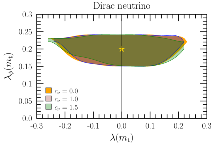
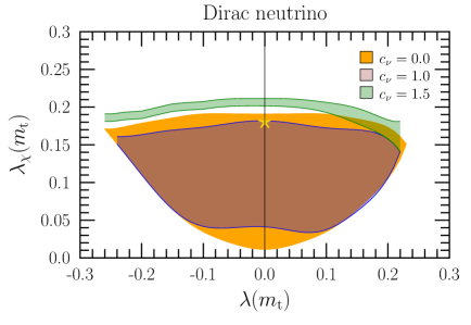
Figure 1: Accepted initial conditions (as shaded areas) in the $\lambda_{\phi}(m_{\mathrm{t}})-\lambda(m_{\mathrm{t}})$ plane (left) and $\lambda_{\chi}(m_{\mathrm{t}})-\lambda(m_{\mathrm{t}})$ plane (right) for the stability of the vacuum and perturbativity preserved up to the Planck mass at different values of the Dirac neutrino Yukawa coupling $c_{\nu}$. The star marks the point in the parameter space for which the example of the running couplings up to the Planck scale is presented in Fig. 2

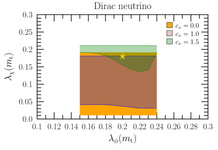
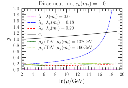
Figure 2: Left: same as Fig. 1 in the $\lambda_{\phi}(m_{\mathrm{t}})-\lambda_{\chi}(m_{\mathrm{t}})$ plane. Right: the running of the couplings up to the Planck scale in a selected point of the parameter space

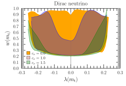
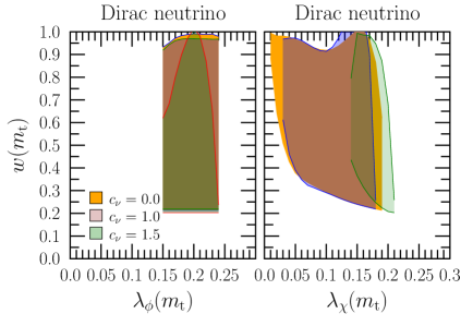
Figure 3: Same as Fig. 1 in the $w(m_{\mathrm{t}})-g(m_{\mathrm{t}})$ planes. Left: $g=\lambda$, right: $g=\lambda_{\phi}$ and $\lambda_{\chi}$

Table 2: Maximal allowed regions of the couplings required by stability of the vacuum and perturbativity of the couplings up to the Planck scale for selected values of the Yukawa coupling of the right-handed neutrino $c_{\nu}(m_{\mathrm{t}})$ and $w<1$ TeV set explicitly

$c_{\nu}$	$\lambda(t)$	$\lambda_{\chi}(t)$	$\!(\mu_{\phi}(t)$/GeV$)^{2}$	$\!(\mu_{\chi}^{2}(t)$/GeV$)^{2}$	$\!w(t)$/GeV	$\!M_{H}(t)$/GeV
0.0	[-0.26,0.23]	[0.011,0.191]	$[-436^{2},496^{2}]$	$[112^{2},580^{2}]$	[213,1000]	[144,558]
1.0	[-0.24,0.22]	[0.031,0.181]	$[-436^{2},436^{2}]$	$[114^{2},548^{2}]$	[220,1000]	[144,557]
1.5	[-0.26,0.22]	[0.141,0.211]	$[-374^{2},496^{2}]$	$[111^{2},603^{2}]$	[203,994]	[144,598]

In this letter we studied the ultraviolet behaviour of a simple, but complete (in the sense of renormalizable quantum field theory) extension of the standard model gauge group Ref. [9]. In order to constrain the parameter space of this new model, its predictions have to be confronted with the large number of established experimental results in particle physics and cosmology. We consider such experimental fact the existence of our Universe, which according to our assumption, requires the stability of the vacuum up to the Planck scale. Thus we computed the $\beta$-functions of the model and studied the dependence of the running couplings of the scalar sector on the scale. Depending on the initial conditions at low energy (set at the mass of the t-quark), we find a region in the parameter space of the new quartic couplings and the largest neutrino Yukawa coupling where the vacuum remains stable up to the Planck scale.

Acknowledgments

This work was supported by grant K 125105 of the National Research, Development and Innovation Fund in Hungary.

Appendix A One-loop $\beta$-functions

We list here the one-loop $\beta$-functions $\beta_{0}\equiv b_{0}/(4\pi)^{2}$ of the $U(1)$-extension of Ref. [9] with the scalar potential in Eq. (4) and for both Dirac neutrinos. If the neutrinos are Majorana type, only the coefficients of the neutrino Yukawa coupling change, which can be found explicitly in Eq. (23). For the $U(1)$-gauge couplings we have

$$\begin{split}b_{0}(g_{Y})&=\frac{41}{6}g_{Y}^{3}\,,\\ b_{0}(g^{\prime}_{Z})&=g^{\prime}_{Z}\biggl{(}\frac{41}{6}g^{\prime}_{ZY}{}^{2}+18g^{\prime}_{Z}{}^{2}+\frac{50}{3}g^{\prime}_{Z}g^{\prime}_{ZY}\biggr{)}\,,\\ b_{0}(g^{\prime}_{ZY})&=g^{\prime}_{ZY}\biggl{(}\frac{41}{6}g^{\prime}_{ZY}{}^{2}+18g^{\prime}_{Z}{}^{2}+\frac{50}{3}g^{\prime}_{Z}g^{\prime}_{ZY}\biggr{)}\,,\end{split}$$ (1)

without using the GUT normalization. The $\beta$-functions of the weak and strong couplings at one-loop level remain the same as in the standard model:

$$b_{0}(g_{\mathrm{L}})=-\frac{19}{6}g_{\mathrm{L}}^{3}\,,\qquad b_{0}(g_{3})=-7g_{3}^{3}\,.$$ (2)

The $\beta$-functions for the Yukawa-couplings are:

$$\begin{split}b_{0}(c_{\nu})&=c_{\nu}\biggl{(}\frac{3}{4}c_{\nu}^{2}-6g^{\prime}_{Z}{}^{2}\biggr{)}\\ b_{0}(c_{\tau})&=c_{\tau}\biggl{(}\frac{5}{2}c_{\tau}^{2}+3c_{\mathrm{t}}^{2}+3c_{\mathrm{b}}^{2}-\frac{9}{4}g_{\mathrm{L}}^{2}-\frac{15}{4}g_{Y}^{2}-\frac{15}{4}g^{\prime}_{ZY}{}^{2}-3g^{\prime}_{Z}{}^{2}-7g^{\prime}_{Z}g^{\prime}_{ZY}\biggr{)}\,,\\ b_{0}(c_{\mathrm{t}})&=c_{\mathrm{t}}\biggl{(}\frac{9}{2}c_{\mathrm{t}}^{2}+\frac{3}{2}c_{\mathrm{b}}^{2}+c_{\tau}^{2}-8g_{3}^{2}-\frac{9}{4}g_{\mathrm{L}}^{2}-\frac{17}{12}g_{Y}^{2}-\frac{17}{12}g^{\prime}_{ZY}{}^{2}-3g^{\prime}_{Z}{}^{2}-3g^{\prime}_{Z}g^{\prime}_{ZY}\biggr{)}\,,\\ b_{0}(c_{\mathrm{b}})&=c_{\mathrm{b}}\biggl{(}\frac{9}{2}c_{\mathrm{b}}^{2}+\frac{3}{2}c_{\mathrm{t}}^{2}+c_{\tau}^{2}-8g_{3}^{2}-\frac{9}{4}g_{\mathrm{L}}^{2}-\frac{5}{12}g_{Y}^{2}-\frac{5}{12}g^{\prime}_{ZY}{}^{2}-3g^{\prime}_{Z}{}^{2}-3g^{\prime}_{Z}g^{\prime}_{ZY}\biggr{)}\,.\end{split}$$ (3)

The scalar mass terms exhibit RG-evolution according to:

$$b_{0}(\mu_{\phi}^{2})=\mu_{\phi}^{2}\biggl{(}12\lambda_{\phi}+2\frac{\mu_{\chi}^{2}}{\mu_{\phi}^{2}}\lambda+2c_{\tau}^{2}+6c_{\mathrm{b}}^{2}+6c_{\mathrm{t}}^{2}-\frac{3}{2}g_{Y}^{2}-\frac{9}{2}g_{\mathrm{L}}^{2}-6g^{\prime}_{Z}{}^{2}-\frac{3}{2}g_{ZY}^{2}-6g^{\prime}_{Z}g^{\prime}_{ZY}\biggr{)}$$ (4)

and

$$b_{0}(\mu_{\chi}^{2})=\mu_{\chi}^{2}\biggl{(}8\lambda_{\chi}+4\frac{\mu_{\phi}^{2}}{\mu_{\chi}^{2}}\lambda+\frac{1}{2}c_{\nu}^{2}-24g^{\prime}_{Z}{}^{2}\biggr{)}$$ (5)

Finally, the $\beta$-functions for the scalar quartic couplings are

$$\begin{split}b_{0}(\lambda_{\phi})&=24\lambda_{\phi}^{2}+\lambda^{2}-2c_{\tau}^{4}-6c_{\mathrm{t}}^{4}-6c_{\mathrm{b}}^{4}+\frac{3}{8}g_{Y}^{4}+\frac{9}{8}g_{\mathrm{L}}^{4}+\frac{3}{4}g_{Y}^{2}g_{\mathrm{L}}^{2}\\ &+6\left(g^{\prime}_{Z}+\frac{g^{\prime}_{ZY}}{2}\right)^{4}+(g_{Y}^{2}+g_{\mathrm{L}}^{2})\left(g^{\prime}_{Z}+\frac{g^{\prime}_{ZY}}{2}\right)^{2}\\ &-\lambda_{\phi}\biggl{[}9g_{\mathrm{L}}^{2}+3g_{Y}^{2}+12\left(g^{\prime}_{Z}+\frac{g^{\prime}_{ZY}}{2}\right)^{2}\biggr{]}+4\lambda_{\phi}\biggl{(}c_{\tau}^{2}+3c_{\mathrm{t}}^{2}+3c_{\mathrm{b}}^{2}\biggr{)}\,,\end{split}$$ (6)

$$b_{0}(\lambda_{\chi})=20\lambda_{\chi}^{2}+2\lambda^{2}-\frac{1}{8}c_{\nu}^{4}+96g^{\prime}_{Z}{}^{2}+\lambda_{\chi}c_{\nu}^{2}-24\lambda_{\chi}g^{\prime}_{Z}{}^{2}$$ (7)

and

$$\begin{split}b_{0}(\lambda)&=12\lambda\lambda_{\phi}+8\lambda\lambda_{\chi}+4\lambda^{2}+48g^{\prime}_{Z}{}^{2}\left(g^{\prime}_{Z}+\frac{g^{\prime}_{ZY}}{2}\right)^{2}+24g_{Y}^{2}g^{\prime}_{Z}{}^{2}\\ &-\lambda\biggl{[}8g^{\prime}_{Z}{}^{2}+\frac{9}{2}g_{\mathrm{L}}^{2}+\frac{3}{2}g_{Y}^{2}+4\left(g^{\prime}_{Z}+\frac{g^{\prime}_{ZY}}{2}\right)^{2}\biggr{]}\\ &+2\lambda\biggl{(}\frac{1}{4}c_{\nu}^{2}+c_{\tau}^{2}+3c_{\mathrm{t}}^{2}+3c_{\mathrm{b}}^{2}\biggr{)}\end{split}$$ (8)

References

• [1] S.Β Weinberg, A Model of Leptons, Phys. Rev. Lett. 19 (1967) 1264–1266.
• [2] ALEPH, DELPHI, L3, OPAL, SLD, LEP Electroweak Working Group, SLD Electroweak Group, SLD Heavy Flavour Group Collaboration, S.Β Schael et.Β al., Precision electroweak measurements on the $Z$ resonance, Phys. Rept. 427 (2006) 257–454 [hep-ex/0509008].
• [3] https://twiki.cern.ch/twiki/bin/view/AtlasPublic/StandardModelPublicResults
• [4] https://twiki.cern.ch/twiki/bin/view/CMSPublic/PhysicsResultsCombined
• [5] ATLAS Collaboration, G.Β Aad et.Β al., Measurement of the Higgs boson mass from the $H\rightarrow\gamma\gamma$ and $H\rightarrow ZZ^{*}\rightarrow 4\ell$ channels with the ATLAS detector using 25 fb-1 of $pp$ collision data, Phys. Rev. D90 (2014), no.Β 5 052004 [1406.3827].
• [6] CMS Collaboration, V.Β Khachatryan et.Β al., Precise determination of the mass of the Higgs boson and tests of compatibility of its couplings with the standard model predictions using proton collisions at 7 and 8  TeV, Eur. Phys. J. C75 (2015), no.Β 5 212 [1412.8662].
• [7] G.Β Degrassi, S.Β DiΒ Vita, J.Β Elias-Miro, J.Β R. Espinosa, G.Β F. Giudice, G.Β Isidori and A.Β Strumia, Higgs mass and vacuum stability in the Standard Model at NNLO, JHEP 08 (2012) 098 [1205.6497].
• [8] D.Β Buttazzo, G.Β Degrassi, P.Β P. Giardino, G.Β F. Giudice, F.Β Sala, A.Β Salvio and A.Β Strumia, Investigating the near-criticality of the Higgs boson, JHEP 12 (2013) 089 [1307.3536].
• [9] Z.Β TrΓ³csΓ‘nyi, Super-weak force and neutrino masses, 1812.11189.
• [10] Particle Data Group Collaboration, M.Β Tanabashi et.Β al., Review of Particle Physics, Phys. Rev. D98 (2018), no.Β 3 030001.
• [11] F.Β del Aguila, M.Β Masip and M.Β Perez-Victoria, Physical parameters and renormalization of U(1)-a x U(1)-b models, Nucl. Phys. B456 (1995) 531–549 [hep-ph/9507455].
• [12] M. E. Peskin, D. V. Schroeder, An introduction to quantum field theory. ABP - The advanced book program. Westview Press, Boulder, Colo. [u.a.], [reprint] edition, [ca. 2007].
• [13] L.Β Basso, Phenomenology of the minimal B-L extension of the Standard Model at the LHC. PhD thesis, Southampton U., 2011. 1106.4462.
• [14] M.Β Gonderinger, H.Β Lim and M.Β J. Ramsey-Musolf, Complex Scalar Singlet Dark Matter: Vacuum Stability and Phenomenology, Phys. Rev. D86 (2012) 043511 [1202.1316].
• [15] N.Β Khan and S.Β Rakshit, Study of electroweak vacuum metastability with a singlet scalar dark matter, Phys. Rev. D90 (2014), no.Β 11 113008 [1407.6015].
• [16] T.Β Alanne, K.Β Tuominen and V.Β Vaskonen, Strong phase transition, dark matter and vacuum stability from simple hidden sectors, Nucl. Phys. B889 (2014) 692–711 [1407.0688].
• [17] S.Β DiΒ Chiara, V.Β Keus and O.Β Lebedev, Stabilizing the Higgs potential with a Zβ€², Phys. Lett. B744 (2015) 59–66 [1412.7036].
• [18] M.Β Duch, B.Β Grzadkowski and M.Β McGarrie, A stable Higgs portal with vector dark matter, JHEP 09 (2015) 162 [1506.08805].
• [19] J.Β Alexander et al., Dark Sectors 2016 Workshop: Community Report, [1608.08632].