K2-288Bb: A Small Temperate Planet in a Low-Mass Binary System Discovered by Citizen Scientists

Abstract

Observations from the Kepler and K2 missions have provided the astronomical community with unprecedented amounts of data to search for transiting exoplanets and other astrophysical phenomena. Here, we present K2-288, a low-mass binary system (M2.0 $\pm$ 1.0; M3.0 $\pm$ 1.0) hosting a small (R_p = 1.9 R_$\earth$), temperate (T_eq = 226K) planet observed in K2 Campaign 4. The candidate was first identified by citizen scientists using Exoplanet Explorers hosted on the Zooniverse platform. Follow-up observations and detailed analyses validate the planet and indicate that it likely orbits the secondary star on a 31.39 day period. This orbit places K2-288Bb in or near the habitable zone of its low-mass host star. K2-288Bb resides in a system with a unique architecture, as it orbits at $>$0.1 AU from one component in a moderate separation binary ($a_{proj}\sim$55 AU), and further follow-up may provide insight into its formation and evolution. Additionally, its estimated size straddles the observed gap in the planet radius distribution. Planets of this size occur less frequently and may be in a transient phase of radius evolution. K2-288 is the third transiting planet identified by the Exoplanet Explorers program and its discovery exemplifies the value of citizen science in the era of Kepler, K2, and TESS.

1 Introduction

With the discovery and validation of over 300 planets spanning the ecliptic as of September 2018, the now retired K2 Mission has continued the exoplanet legacy of Kepler by providing high-cadence continuous light curves for tens of thousands of stars for more than a dozen $\sim$80 day observing campaigns (Howell et al., 2014; NASA Exoplanet Archive, 2018). The surge of data, with calibrated target pixel files from each campaign being publicly available approximately three months post-observing, is processed and searched by the astronomy community for planetary transits. However, due to spacecraft systematics and non-planetary astrophysical signals (e.g. eclipsing binaries, pulsations, etc.) that could be flagged as potential planets, all transiting candidates are vetted by-eye before proceeding with follow-up observations to validate and characterize the system.

Because thousands of signals are flagged as potential transits, by-eye vetting is a necessary, however tedious, task (e.g. Crossfield et al., 2016; Yu et al., 2018; Crossfield et al., 2018). Transits can also be missed and the lowest signal-to-noise events are often not examined. This presents the opportunity to source the search for transiting planets and other astrophysical variables in K2 data to the public, leveraging the innate human ability for pattern recognition and interest to be involved in the process of exoplanet discovery. The Planet Hunters citizen science project (Fischer et al., 2012; Schwamb et al., 2012), hosted by the Zooniverse platform (Lintott et al., 2008), pioneered the combination of Kepler and K2 time series data and crowd sourced searches for exoplanets and other time variable phenomena. Planet Hunters has been hugely successful, with more than ten refereed publications presenting discoveries of new planet candidates, planets, and variables (e.g. Gies et al. (2013); Schmitt et al. (2014); Wang et al. (2013)); this includes surprising discoveries such as the enigmatic “Boyajian’s Star” (KIC 8462852, Boyajian et al., 2016) as well.

Building on the success of Planet Hunters, the Exoplanet Explorers program invites citizen scientists to discover new transiting exoplanets from K2. Exoplanet Explorers presents processed K2 time series photometry with potential planetary transits as a collage of simple diagnostic plots and asks citizen scientists to cycle through the pre-identified candidates and select those matching the expected profile of a transiting exoplanet. Flagged candidates are then examined by the Exoplanet Explorers team and the most promising are prioritized for follow-up observations to validate the systems. When Exoplanet Explorers was launched, candidate transits were uploaded as soon as planet searches in new K2 campaigns had completed and citizen scientists were examining these new candidates simultaneously with our team. This process began with K2 Campaign 12 and Exoplanet Explorers immediately had success with its first discovery, K2-138, a system hosting five transiting sub-neptunes in an unbroken chain of near 3:2 resonances (Christiansen et al., 2018). Another system simultaneously identified by our team and citizen scientists on Planet Hunters and Exoplanet Explorers is K2-233, a young K dwarf hosting three small planets (David et al., 2018). Following the K2-138 discovery, we also made available candidates from K2 campaigns observed prior to the launch of Exoplanet Explorers. This allowed for the continued vetting of low signal-to-noise candidates and the opportunity to identify planets that may have been missed our team’s vetting procedures.

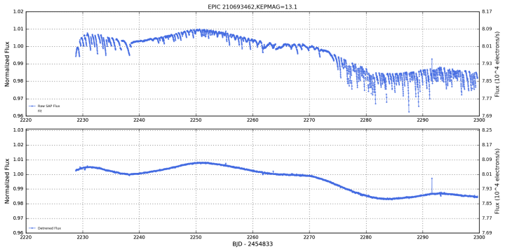
Figure 1: Top: Raw K2 photometry of EPIC 210693462 displaying time and roll dependent spacecraft systematics. Bottom: systematics corrected, detrended light curve.

Here we present an example of such a system: K2-288 from K2 Campaign 4, the third discovery by the citizen scientists of Exoplanet Explorers. K2-288 is a small ($\sim$ 1.90$~{}R_{\earth}$) temperate (T$\sim$226 K) planet orbiting one component of a nearby M dwarf binary. We layout the validation of the system in the following way: In  § 2, we describe the K2 observations and discovery of the candidate by citizen scientists. We describe follow-up observations and the detection of an M-dwarf stellar secondary in  § 3. In  § 4, we discuss Gaia DR2 and Spitzer follow-up observations, and we discuss transit analyses, estimated planet parameters, and system validation in  § 5. We conclude with  § 6, which summarizes our final remarks on the system and expresses the importance of citizen scientists for future exoplanet discoveries.

2 K2 Observations and Candidate Identification

K2-288 (EPIC 210693462, LP 413-32, NLTT 11596, 2MASS J03414639+1816082) was proposed as a target in K2 Campaign 4 (C4) by four teams in K2 GO Cycle 1. The target was subsequently observed at 30-minute cadence for 75 days in C4, which ran from 2015 February 7 until 2015 April 23. Following our team’s previous work (Crossfield et al., 2016; Petigura et al., 2018; Yu et al., 2018), we used the publicly available k2phot software package (Petigura et al., 2015) to simultaneously model spacecraft systematics and stellar variability to detrend all C4 data. Periodic transit like signals were then identified using the publicly available TERRA algorithm (Petigura et al., 2013a, b). In this initial search of the detrended EPIC 210693462 light curve, TERRA did not identify any periodic signals with at least three transits. Subsequently, all C4 data was re-processed using an updated version of k2phot (see Fig. 1) and searched again for transit like signals using TERRA. Transit candidates from these re-processed light curves were uploaded to Exoplanet Explorers. Citizen scientists participating in the project identified a previously unrecognized candidate transiting K2-288 (see Fig. 2).

Citizen scientists of the Exoplanet Explorers project are presented with a portion of a TERRA processed K2 light curve. The presentation includes a light curve folded onto the phase of the candidate transit and a stack of the individual transit events (Fig. 2). After a brief introduction, users are asked to examine the light curve diagnostic plots and select candidates that have features consistent with a transiting planet. Sixteen citizen scientists identified the candidate transiting K2-288 as a candidate of interest. The newly identified candidate transited just three times during K2 C4 with a period of approximately 31 days. In the discussion forums of Exoplanet Explorers, some of the citizen scientists used preliminary stellar (from the EPIC, Huber et al., 2016) and planet (from the TERRA output) parameters to estimate that the transiting candidate was approximately Earth sized and the incident stellar flux it received was comparable to the flux received by the Earth, increasing our interest in the system.

Through Zooniverse, we contacted the citizen scientists who flagged this system as a potential transit. Many were pleasantly surprised and excited to hear that they were able to contribute to the scientific community. Additionally, they were very appreciative of our reaching out and giving them the opportunity to receive credit for their contributions and participate in this work. 50% of those citizen scientists involved responded to our email and are included as co-authors on this publication; the rest are thanked in the acknowledgements. We aim to continue the precedent set by Christiansen et al. (2018) of attributing credit to all, including citizen scientists, who are involved in planetary system identification and validation.

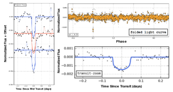
Figure 2: Collage of vetting diagnostics for K2-288 presented to citizen scientists on Exoplanet Explorers. The left image shows a stack of the individual transits with arbitrary flux offsets and alternating model fit colors for clarity. The top right image is the full K2 light curve folded onto the period of the transit like signal. The small black points are the K2 data, the orange circles are binned. The bottom right is a zoom on the transit in the period folded light curve with a preliminary planet model in blue. The detection of three transits with consistent shapes and depths and a folded transit with a planet like profile led citizen scientists to flag this event as a candidate planet.

After the discovery by citizen scientists, we investigated the full k2phot light curve and the TERRA outputs to understand how this intriguing candidate was overlooked in our catalog of planets and candidates from the first year of K2 (Crossfield et al., 2016). Our investigation revealed that the candidate was missed by our first analysis of the K2 C4 light curves because the version of the k2phot software used trimmed data from the beginning and end of the observing sequence. This is a common practice to mitigate systematics at the start and finish of a K2 campaign. The first transit, occurring only 2 days into the observing sequence, was trimmed from the data prior to running TERRA and the algorithm did not flag the candidate because it only transited twice (see Fig. 9). We searched additional publicly available light curves of K2-288 on the Mikulski Archive for Space Telescopes (MAST) for a similar transiting candidate. Due to data trimming similar to that applied to our original k2phot light curve, the k2sff (Vanderburg & Johnson, 2014) light curve also exhibited only two transits and the candidate was not published in the catalog of Mayo et al. (2018). However, three transits were recovered in the EVEREST (Luger et al., 2016, 2017) and k2sc (Aigrain et al., 2016) light curves but the candidate and its parameters have not yet been published. Following these checks, we compiled known information on the system (see Table 1) and began follow-up observations to further characterize the host star and validate the candidate planet.

3 Ground Based Observations

3.1 IRTF SpeX

The first step in our follow-up process was observing K2-288 with the near-infrared cross-dispersed spectrograph, SpeX (Rayner et al., 2003, 2004) on the 3-meter NASA Infrared Telescope Facility. The observations were completed on 2017 July 31 UT (Program 2017A019, PI C. Dressing). The target was observed under favorable conditions, with an average seeing of $\sim$0.8^′′. We used SpeX in its short cross-dispersed mode (SXD) with the 0.3$\times$15^′′ slit, covering 0.7-2.55 $\mu$m at a resolution of R $\sim$ 2000. The target was observed for an integration time of 120s per frame at two locations along the slit in 3 AB nod pairs, leading to a total integration time of 720s. The slit position angle was aligned to the parallactic angle in order to minimize differential slit losses. After observing K2-288, we immediately observed a nearby A0 standard, HD23258, for later telluric correction. Flat and arc lamp exposures were also taken for wavelength calibration. The spectrum was reduced using the SpeXTool package (Vacca et al., 2003; Cushing et al., 2004).

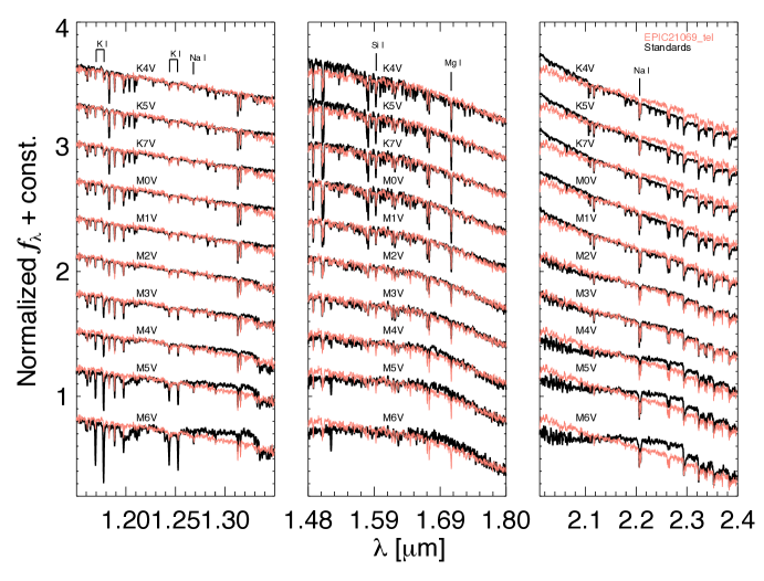
Figure 3: The $JHK$-band spectra of K2-288 (EPIC 210693462) obtained using SpeX on the IRTF (salmon) compared to late-type dwarf standards from the IRTF spectral library (black). All spectra are normalized to the continuum in each of the plotted regions. After processing using SpeXTool, the resulting spectra is a best visual match to the M2/M3 spectral type across the three $JHK$-bands.

SpeXTool uses the obtained target spectra, A0 standard spectra, and flat and arc lamp exposures to complete the following reductions: flat fielding, bad pixel removal, wavelength calibration, sky subtraction, and flux calibration. The package yields an extracted and combined spectra. The resulting two spectra have signal-to-noise ratios (SNRs) of 106 in the J-band ($\sim$1.25 $\mu$m), 127 in the H-band ($\sim$1.6 $\mu$m), and 107 per resolution in the K-band ($\sim$2.2 $\mu$m). The reduced spectra is compared to late-type standards from the IRTF Spectral Library (Rayner et al., 2009) across the JHK-bands in Figure  3. Upon visual inspection, K2-288 is an approximate match to the M2/M3 standard across all three bands. This is consistent with the spectral type estimated using the NIR index based H${}_{2}0_{K2}$ method of Rojas-Ayala et al. (2012), M2.0 $\pm$ 0.6, and the optical index based TiO5 and CaH3 methods of Lépine et al. (2013), M3.0 $\pm$ 0.5.

We used the SpeX spectrum to approximate the fundamental parameters of the star (metallicity, [Fe/H]; effective temperature, $T_{\mathrm{eff}}$; radius, $R_{*}$; mass, $M_{*}$; and luminosity, $L_{*}$) following the prescription presented in Dressing et al. (2017). Specifically, we estimate the stellar $T_{\mathrm{eff}}$, $R_{*}$, and $L_{*}$ using the relations of Newton et al. (2015), the metallicity using the relations of Mann et al. (2013a), and $M_{*}$ by using the Newton et al. (2015) $T_{\mathrm{eff}}$ in the temperature-mass relation of Mann et al. (2013b). Newton et al. (2015) used a sample of late-type stars with measured radii and precise distances to develop a relationship between the equivalent widths of $H$-band Al and Mg lines and fundamental parameters. Mann et al. (2013a) used a set of wide binaries with solar type primaries and M dwarf companions to calibrate a relationship between metallicity and the strength of metallicity sensitive spectroscopic indices. Mann et al. (2013b) derived an empirical effective temperature relationship using a sample of low-mass stars with measured radii and distances and temperature sensitive indices in the near infrared spectra of low-mass stars. Using the same samples, they then derived additional empirical relations for $T_{\mathrm{eff}}$-$R_{*}$, $T_{\mathrm{eff}}$-$M_{*}$, and $T_{\mathrm{eff}}$-$L_{*}$. Our application of these empirical relationships to the SpeX spectrum of K2-288 following the prescription of Dressing et al. (2017) results in $T_{\mathrm{eff}}$ = 3479 $\pm$ 85 K, $R_{*}$ = 0.47 $\pm$ 0.03 $R_{\odot}$, $M_{*}$ = 0.38 $\pm$ 0.08 $M_{\odot}$, log($L/L_{*}$) = -1.53 $\pm$ 0.06, and [Fe/H] = -0.06 $\pm$ 0.21. The estimated stellar parameters are consistent with the M2.5 spectral type measured from the spectrum. We note that these values apply to the blended spectrum of a binary system and are not indicative of the final stellar parameters for the components in the system. We discuss the discovery and properties of the binary in  § 3.2, 3.3, and 5.3.

3.2 Keck HIRES

We observed K2-288 on 2017 Aug 18 UT with the HIRES spectrometer (Vogt et al., 1994) on the Keck I telescope. The star was observed following the standard California Planet Survey (CPS, Marcy et al., 2008; Howard et al., 2010) procedures with the C2 decker, $0\farcs 87\times 14\farcs 0$ slit, and no iodine cell. This set-up provides wavelength coverage from 3600 - 8000 Å at a resolution of $R\approx 60,000$. We integrated for 374s, achieving 10,000 counts on the HIRES exposure meter for an SNR of $\sim$25 per pixel at 5500 Å. The target was observed under favorable conditions, with seeing $\sim$ 1^′′. During these observations, we noted that the intensity distribution of the source in the HIRES guider images was elongated approximately along the SE-NW axis. We observed K2-288 again on 2017 Aug 19 UT using the same instrument settings and integration time, but in slightly better seeing. A secondary component was partially resolved in the guider images at $\sim$1^′′ to the SE. This observation prompted adaptive optics imaging using Keck NIRC2 to fully resolve the binary (see § 3.3). Following the identification of the secondary, we observed K2-288 again with Keck HIRES on 2017 Sept 6 UT with an integration time of 500s in $<1^{\prime\prime}$ seeing, achieving an SNR $\sim$20 per pixel at 5500 $\AA$. During these observations, we oriented the slit to be perpendicular to the binary axis (PA = 330^∘) and shifted the slit position to center it on the secondary (K2-288B). All HIRES spectra were reduced using standard routines developed for the California Planet Survey (Howard et al., 2010, CPS).

Visual inspection of the reduced blended and secondary spectra revealed morphologies and features consistent with low activity M dwarfs. All spectra exhibited H$\alpha$ absorption, with no discernible emission in the line cores or wings. Weak emission cores were visible in the Ca II H&K lines, however we did not measure their strengths due to the very low SNR ($\leq$3) at short wavelengths. Such weak emission is often observed even in low-activity M dwarfs. We derived stellar parameters from the spectra using the SpecMatch-Emp code (Yee et al., 2017). SpecMatch-Emp is a software tool that uses a diverse spectral library of $\sim$400 well-characterized stars to estimate the stellar parameters of an input spectrum. The library is made up of HIRES spectra taken at high SNR($>$100 per pixel). SpecMatch-Emp finds the optimum linear combination of library spectra that best matches the unknown target spectrum and interpolates the stellar $T_{\mathrm{eff}}$, $R_{*}$, and [Fe/H]. SpecMatch-Emp performs particularly well on stars with $T_{\mathrm{eff}}$ $<$4700 K, so it is well suited to K2-288, a pair of M dwarfs. SpecMatch-Emp achieves an accuracy of 70 K in $T_{\mathrm{eff}}$, 10% in $R_{*}$, and 0.12 dex in [Fe/H] (Yee et al., 2017). The library parameters are derived from model-independent techniques (i.e. interferometry or spectrophotometry) and therefore do not suffer from model-dependent offsets associated with low-mass stars (Newton et al., 2015; Dressing et al., 2017). Our SpecMatch-Emp analysis of the blended spectra resulted in mean parameters of $T_{\mathrm{eff}}$ $=3593\pm 70$ K, $R_{*}=0.44\pm 0.10R_{\odot}$, and [Fe/H] = -0.29 $\pm$ 0.09. Consistent with an M2.0 $\pm$ 0.5 spectral type following the color-temperature conversions of Pecaut & Mamajek (2013). The SpecMatch-Emp analysis of the secondary spectrum resulted in $T_{eff}=3456\pm 70$ K, $R_{*}=0.41\pm 0.10R_{\odot}$, and [Fe/H] = -0.21 $\pm$ 0.09. The spectroscopic temperature of the secondary is approximately 150K cooler than the blended spectrum. This is consistent with an M3.0 $\pm$ 0.5 spectral type (Pecaut & Mamajek, 2013). The HIRES stellar parameters for the blended spectrum are also consistent with the SpeX parameters within uncertainties. Since the HIRES spectra are blended or only partially resolved, we only use the metallicities in subsequent analyses. As expected for stars in a bound system, the metallicities from the different spectra are consistent. The measured metallicities are provided in Table 1.

The standard CPS analyses of the HIRES spectra also provide barycentric corrected radial velocities (RV). Our two epochs of blended HIRES spectra provide a mean RV of $73.0\pm 0.3$ km s^-1. The partially resolved secondary spectrum yields RV = $70.2\pm 0.3$ km s^-1. These RVs are broadly consistent but differ at the 9$\sigma$ level, potentially due to orbital motion. To search for additional stellar companions at very small separations, we performed the secondary line search algorithm presented by Kolbl et al. (2015) on the HIRES spectra. This analysis did not reveal any significant signals attributable to additional unseen companions in the system at $\Delta$RV $\geq$ 10 km s^-1 and $\Delta$$V$$\lesssim$ 5 mag. We report the weighted mean HIRES RV in Table 1.

3.3 High-resolution Imaging

After the binary companion was identified, we observed K2-288 with high-resolution adaptive optics (AO) imaging at the Keck Observatory. This was completed in order to ensure our transit signal was due to the presence of an exoplanet and not the stellar companion. The observations were made on Keck-II with the NIRC2 instrument behind the natural guide star AO system. These observations were completed on 2017 Aug 20 UT in the standard 3-point dither pattern used with NIRC2. This observing mode was chosen to avoid the typically noisier lower left quadrant of the detector. We observed K2-288 in the narrow-band $Br-\gamma$, the H-continuum, and J-continuum filters. Using a step-size of $3\arcsec$, the dither pattern was repeated three times, with each dither offset from the previous by 0.5$\arcsec$. We used integration times of 6.6, 4.0, and 2.0s, for the the narrow-band $Br-\gamma$, the H-continuum, and J-continuum respectively, with the co-add per frame for a total of 59.4, 36.0, and 26.1s. The narrow-angle mode of the camera allowed for a full field of view of $10\arcsec$ and a pixel scale of approximately $0.009942\arcsec$ per pixel. The Keck AO observations clearly detected a nearly equal brightness secondary $\sim 0.8\arcsec$ to the southeast of the primary target. We also observed K2-288 on 2017 Dec 29 UT in the broader $J$ and $K_{p}$ filters through poor and variable seeing ($\sim$1-2^′′). The binary was clearly resolved, but the images were of much lower quality than the 2017 Aug 20 observations and are not used in any subsequent analyses.

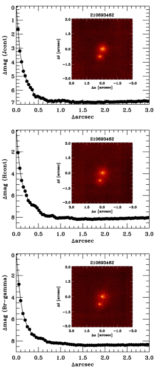
Figure 4: Contrast sensitivities and Keck/NIRC2 AO images (insets) of K2-288 in the $Jcont$, $Hcont$, and $Br-\gamma$ filters. A secondary secondary is clearly detected at $\sim$0.8” in each band. The 5$\sigma$ contrast limits for additional secondarys are plotted against angular separation in arcseconds for each filter; the black points represent one step in the FWHM resolution of the images.

The resulting NIRC2 AO data have a resolution of 0.049^′′ (FWHM) in the $Br$-$\gamma$ filter, 0.040^′′ (FWHM) in the $H$-$cont$, and 0.039^′′ (FWHM) in the $J$-$cont$ filter. Fake sources were injected into the final combined images with separations from the primary in multiples of the central source’s FWHM in order to derive the sensitities of the data (Furlan et al., 2017). The $5\sigma$ limits on the sensitivity curves are shown in Figure 4. The separation of the secondary was measured from the $Br$-$\gamma$ image and determined to be $\Delta\alpha=0.259\arcsec\pm 0.001\arcsec$ and $\Delta\delta=-0.746\arcsec\pm 0.001\arcsec$, corresponding to a position angle of PA $\approx 159.8^{\circ}$ east of north. The blending caused by the presence of the secondary was taken into account in the resulting analysis, to obtain the correct transit depth and planetary characteristics (Ciardi et al., 2015).

The blended 2MASS $JHK$-magnitudes of the system are: $J=10.545\pm 0.020$ mag, $H=9.946\pm 0.023$ mag, and $K_{s}=9.724\pm 0.018$ mag. The primary and secondary have measured magnitude differences of $\Delta J=0.997\pm 0.009$ mag, $\Delta H=0.990\pm 0.005$ mag, and $\Delta K_{s}=0.988\pm 0.004$ mag. $Br$-$\gamma$ has a central wavelength that is sufficiently close to $Ks$ to enable the deblending of the 2MASS magnitudes into the two components. The primary star has deblended real apparent magnitudes of $J_{1}=10.910\pm 0.027$ mag, $H_{1}=10.313\pm 0.021$ mag, and $Ks_{1}=10.092\pm 0.023$ mag, corresponding to $(J-H)_{1}=0.597\pm 0.033$ mag and $(H-K_{s})_{1}=0.221\pm 0.031$ mag. The secondary star has deblended real apparent magnitudes of $J_{2}=11.907\pm 0.0269$ mag, $H_{2}=11.303\pm 0.021$ mag, and $Ks_{2}=11.079\pm 0.023$ mag, corresponding to $(J-H)_{2}=0.604\pm 0.033$ mag and $(H-K_{s})_{2}=0.223\pm 0.031$ mag. We derived the approximate deblended Kepler magnitudes of the two components using the $(Kepmag-Ks)\ vs.\ (J-Ks)$ color relationships described in Howell et al. (2012). The resulting deblended Kepler magnitudes are $Kep_{1}=13.46\pm 0.09$ mag for the primary and $Kep_{2}=14.49\pm 0.10$ mag for the secondary, with a resulting Kepler magnitude difference of $\Delta Kep=1.03\pm 0.12$ mag. These deblended magnitudes were used when fitting the light curves and deriving true transit depth.

Both stars have infrared colors that are consistent with approximately M3V spectral type (Figure 5). However, this is driven by the uncertainties on the component photometry. With an approximate primary spectral type of M2, and $\Delta$$JHK$$\approx$1 mag, the secondary is likely about one and half sub-types later than the primary (Pecaut & Mamajek, 2013). It is unlikely that the star is a heavily reddened background star. Based on an extinction law of $R=3.1$, an early-K type star would have to be attenuated by more than 1 magnitude of extinction for it to appear as a mid M-dwarf. The line-of-sight extinction through the Galaxy is only $A_{V}\approx 0.7$ mag at this location (Schlafly & Finkbeiner, 2011), making a highly reddened background star unlikely compared to the presence of a secondary companion. Additionally, archival ground based imaging does not reveal a stationary or slow moving point source near the current location of K2-288, indicating that the imaged secondary at 0.8” is likely bound (See § 3.4). Gaia DR2 also provides consistent astrometry for two stars near the location of K2-288 (See § 4.1).

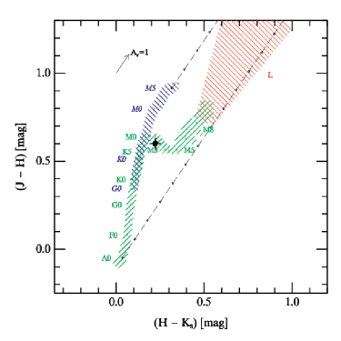
Figure 5: 2MASS $JHK_{s}$ color-color diagram of the dwarf branch locus (green; Carpenter (2001), Hawley et al. (2002)), the giant branch locus (blue; Carpenter (2001)), and the brown dwarf locus (red; Kirkpatrick et al. (2000), Burgasser et al. (2002)). $A_{V}$, the direction of reddening due to extinction, is represented by the black dashed lines. The positions of the K2-288 components are over plotted. The primary and secondary are both consistent with $\sim$M3V spectral types.

3.4 Seeing Limited Archival Imaging

K2-288 is relatively bright and has been observed in many seeing limited surveys at multiple wavelengths. Currently available archival imaging of the system spans nearly 65 years. Over the long time baseline of the available imaging, the large total proper motion of K2-288 ($\mu$ = 195.9 mas yr^-1) has carried it $\approx$12$\farcs$5. This allows for additional checks for very close background sources at the current location of the system and additional constraints on whether the resolved binary is bound or a projected background source. Figure 6 displays an image of K2-288 from K2 at its current location (left) compared to two epochs of Palomar Observatory Sky Survey (POSS) images (center and right). The green polygon represents the optimal photometric aperture used to extract the K2 light curve. In the POSS images from 1951, there is no source at K2-288’s current location down to the POSS I $R$ limit of 20.0 mag (Abell, 1966). This indicates that there are no slow moving background stars that are beyond the limits of our AO imaging. Additionally, the lack of a bright source at the current location in archival observations reinforces that the resolved secondary is bound and co-moving with the primary.

The archival data does reveal a faint point source $\sim$14^′′ to the NE of K2-288’s current location. This star, 2MASS J03414730+1816135, is relatively slow moving ($\mu$ = 32.6 mas yr^-1) background source at a distance of 390 pc (Gaia Collaboration et al., 2018). It is $\sim$5 magnitudes fainter than K2-288 in the Kepler band and falls just outside of the optimal aperture used to produce the K2 light curve. Due to its proximity to the optimal aperture, this background star warrants further examination as the potential source of the transit signal. We used additional light curves generated during the k2phot reduction where the flux was extracted using different size apertures to investigate possible contributions from this faint star. In Figure 7 we show the phase folded transit signal from the light curve extracted with the optimal aperture compared to the same signal extracted using soft-edged circular apertures with radii of 1.5, 3, and 8 pixels. Due to the proper motion of the target and the use of 2MASS coordinates to place the circular apertures, the centers are offset from K2-288’s current position by $\sim$3^′′. None the less, the 3 and 8 pixel radius apertures yield phase folded transits with the same approximate depth as the optimal aperture while including more light from the nearby faint background star. The 1.5 pixel circular aperture suffers from a substantial increase in noise because it does not include the brightest pixels of K2-288. These analyses indicate that the faint slow moving background star is likely not the source of the observed transits and the candidate orbits one of the components of resolved binary. This is further reinforced by our detection of a partial transit in Spitzer observations that use an aperture that is much smaller and free of contamination from the faint nearby star (see § 4.2).

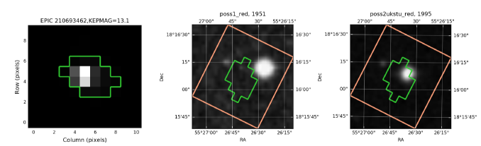
Figure 6: Archival imaging data for K2-288. The left panel is the data from K2 in 2015 with the k2phot optimal photometric aperture overlaid in green. The center panel is a POSS I $R_{POSS}$-band image from 1951. The right panel is a POSS II $R_{POSS}$-band image from 1995. The optimal aperture is translated into the POSS image coordinates for comparison. K2-288 has moved substantially over the nearly 65 years covered by the images. The lack of a bright star at the current position of K2-288 in the past images indicates that there are no background sources at its current position that remain unresolved in our AO imaging observations and that the imaged companion is co-moving with the primary. We also note the faint, slow moving background source just to the NE of the optimal aperture in the POSS images. Analysis of the transit depth using different size apertures indicates that this star is not the source of the transit signal.

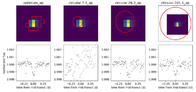
Figure 7: The phase folded transit signal for K2-288, extracted with the optimal aperture compared and the same signal extracted using soft-edged circular apertures with radii of 1.5, 3, and 8 pixels. The proper motion of the target and the use of 2MASS coordinates to place the apertures causes the circular apertures to be slightly offset from the center. Regardless of this offset, the optimal and 3 and 8 pixel circular apertures recover transits with consistent depths and indicate that the candidate planet transits one of the components of K2-288, not the nearby faint background star detected in archival ground based images.

4 Space Based Observations

4.1 Gaia DR2

Astrometry (Lindegren et al., 2018) and photometry (Riello et al., 2018; Evans et al., 2018) of K2-288 obtained by Gaia over the first twenty-two months of mission operations were made available in the second data release from the mission (DR2 Gaia Collaboration et al., 2018). The DR2 catalog lists two sources within 3$\farcs$7 of the 2MASS coordinates of K2-288 (Gaia DR2 44838019758175488 and 44838019756570112). The separation, position angle, and $\Delta G$ of these sources are consistent with the results of our Keck AO imaging and the estimated magnitude difference in the Kepler band. Thus, both components of K2-288 were resolved by Gaia. However, the proximity of the sources led to relatively poor fits in the 5-parameter astrometric solution for each star. Here we refer to the goodness of fit statistic of the astrometric solution in the along scan direction, astrometric_gof_al in the Gaia DR2 catalog. Good solutions typically have $astrometric\_gof\_al<3$, where K2-288 A and B have values of 24.1 and 31.8, respectively. This also leads to significant excess noise in the fit for each star (Gaia DR2 parameter astrometric_excess_noise), 0.41 mas for the primary and 0.77 mas for the secondary. The utility of Gaia DR2 data in identifying binaries has been demonstrated via comparison to a large sample of AO resolved multiple systems from the Kepler planet candidate host sample (Ziegler et al., 2018). Similarly significant excess noise in Gaia astrometric parameter fits has also been observed in this sample (Rizzuto et al., 2018).

The astrometric statistics of K2-288 may be improved in later Gaia data releases as more data is obtained for each star. The excess errors are manifested as discrepancies between the astrometric measurements of the components. For example, the parallax of the secondary differs from that of the primary by 0.9 mas, a $>4\sigma$ difference (when considering the secondary parallax uncertainty). This discrepancy is likely too large to be attributed to binary orbital motion over the time baseline of the Gaia observations.

Despite this discrepancy, the distances to the components of the binary are comparable, $70.0\pm 0.4$ pc and $65.7\pm 0.9$ pc for the primary and secondary, respectively. Given supporting evidence that these stars form a moderate separation, bound system – consistent RVs (see § 3.2), consistent proper motions (see § 3.4) – we adopt the weighted mean and error of the primary and secondary distances as the distance to the system, $69.3\pm 0.4$ pc, and include it in Table 1. At this adopted distance, we find the projected separation of the secondary is $54.8\pm 0.4$ AU. We also use this distance to infer the individual stellar parameters of the components in § 5.3. Gaia DR2 also provides a radial velocity for the primary, RV = $72.15\pm 1.72$ km s^-1. This is consistent with the HIRES measured system RV and provides further evidence that there are not additional unseen stellar companions in the system.

4.2 Spitzer Space Telescope Observations

EPIC 210693462 was observed by Spitzer from UT 2017-12-11 15:35:58 to 2017-12-11 20:31:28. The observations were conducted with the Infra-Red Arracy Camera (IRAC; Fazio et al. 2004) at 4.5 µm  with an exposure time of 2 seconds. Because of the small separation of the binary components ($\sim$0.8″) and the pixel scale of IRAC (1.2″), the binary was unresolved in the Spitzer images. Photometry of the blended binary PSF was obtained using circular apertures and the background was estimated and subtracted following a procedure similar to Beichman et al. (2016). The aperture was then chosen by selecting the light curve with minimal white and red noise statistics, as computed by the standard deviation and the red noise factor $\beta$ (Pont et al. 2006, Winn et al. 2008, Livingston et al. in review). Following this procedure, an aperture radius of 2.3 pixels was found to yield the lowest noise, which is consistent with the optimal apertures found in previous studies (e.g. Beichman et al., 2016; Knutson et al., 2012). We then binned the light curve and pixel data to 60 seconds, as this has been shown to yield an improved systematics correction without affecting the information content of the light curve (e.g. Benneke et al., 2017).

5 System Properties & Validation

5.1 Individual Component Properties

Due to the close separation of the components of K2-288, it is crucial to estimate their individual properties to further evaluate the characteristics of the planet candidate. The spectra obtained using HIRES and SpeX are blended and the stellar parameters estimated in §’s 3.1 and 3.2 are not indicative of the properties of each star, except the metallicities, which should be, and are measured to be, consistent. However, our resolved NIR photometry from Keck AO imaging and the Gaia distance to the system provide a basis for reliably estimating the individual component properties.

We base our approach on that of Dressing et al. (2018), which hinges on using stellar absolute $K_{s}$ magnitudes ($M_{K}$), photometric colors, and calibrated relations to estimate the masses, radii, and effective temperatures of low-mass stars. Dressing et al. (2018) showed that this approach provides fundamental parameter estimates consistent with those calculated using spectroscopic index and equivalent width based relations with comparable levels of precision. We used the adopted system distance of $69.3\pm 0.4$ pc and the resolved $K_{s}$-band magnitudes of the components to calculate their $M_{k}$’s. We find $M_{K_{p}}=5.888\pm 0.036$ mag for the primary and $M_{K_{s}}=6.875\pm 0.036$ mag for the secondary. Throughout the discussion, we use the subscript $p$ to denote the primary and $s$ to denote the secondary.

To estimate the masses of the stars, we used the $M_{K}$ - mass relation presented in Benedict et al. (2016). We estimated stellar mass uncertainties by assuming the errors on our absolute magnitudes and the coefficients in Benedict et al. polynomial relation follow Gaussian distributions and calculated the mass 10⁴ times using Monte Carlo (MC) methods. The median and standard deviation of the resulting distribution were adopted as the mass and associated statistical uncertainty. We then added this uncertainty in quadrature to the intrinsic scatter in the Benedict et al. (2016) relation (0.02 $M_{\odot}$). This procedure resulted in mass estimates of $M_{p}=0.52\pm 0.02M_{\odot}$and$M_{s}=0.33\pm 0.02M_{\odot}$.

Our radii estimates use the $M_{K}$ - radius - $[$Fe/H$]$ relation from Mann et al. (2015, 2016). In these calculations we used the HIRES measured metallicities attributed to the primary and secondary provided in Table 1. Our approach to radius uncertainty estimates is similar to that used in the mass calculation. We use MC methods assuming Gaussian distributed errors on $M_{K}$ and $[$Fe/H$]$ then add the resulting radius uncertainties in quadrature to the scatter in the Mann et al. (2015, 2016) polynomial fit (0.027 $R_{\odot}$). This results in radii estimates of $R_{p}=0.45\pm 0.03R_{\odot}$ and $R_{s}=0.32\pm 0.03R_{\odot}$.

Our effective temperature estimates use the $V-J$ - $\mathrm{T_{eff}}$ - $[$Fe/H$]$ relation from Mann et al. (2015, 2016). Here we also used the HIRES measured metallicities from Table 1. The calculation also requires an estimate of the $V-J$ color of the stars, which we interpolate from the Pecaut & Mamajek (2013) main sequence color-temperature table. The $V-J$ color and uncertainty is estimated using MC methods during the interpolation. We estimate $(V-J)_{p}=3.304\pm 0.022$ mag for the primary and $(V-J)_{s}=3.962\pm 0.024$ mag for the secondary. We then used the Mann et al. (2015, 2016) relation to estimate the stellar temperatures following the same approach to uncertainty estimation previously described for the mass and radius estimates. We estimate the primary and secondary effective temperatures to be $\mathrm{T_{eff,p}=3584\pm 205}$ K and $\mathrm{T_{eff,s}=3341\pm 276}$ K, respectively. These effective temperatures are consistent with spectral types of M2 $\pm$ 1 and M3 $\pm$ 1 using the relations of Pecaut & Mamajek (2013). Additionally, the temperature estimated using the resolved primary photometry is consistent with the temperatures estimated from the blended SpeX and HIRES spectra (see §’s 3.1 and 3.2). This result is consistent with the $\sim$1 magnitude difference between the components inferred from Keck AO imaging which reveals that the primary contributes substantially more flux than the secondary and dominates the blended spectra. We also use our calculated $M_{K}$ mags and the Pecaut & Mamajek (2013) extended table to interpolate luminosities for K2-288 A and B. These values, along with all of the other stellar parameters, are included in Table 1. The parameters estimated in this section are used in subsequent transit modeling analyses.

5.2 Transit Analyses

5.2.1 K2 and Spitzer Transit Modeling

To model the K2 transit, we adopted a Gaussian likelihood function and the analytic transit model of Mandel & Agol (2002) as implemented in the Python package batman (Kreidberg, 2015). We used the Python package emcee (Foreman-Mackey et al., 2013) for Markov Chain Monte Carlo (MCMC) exploration of the posterior probability surface. The free parameters of the transit model are: the planet-to-star radius ratio $R_{p}/R_{\star}$, the scaled semi-major axis $a/R_{\star}$, mid transit time $T_{0}$, period $P$, impact parameter $b$, and the quadratic limb darkening coefficients $q_{1}$ and $q_{2}$ under the transformation from $u$-space of Kipping (2013). The transit signal was originally identified in the k2phot light curve. However, for this analysis, we fit the transit model to the EVEREST 2.0 (Luger et al., 2017) light curve due to the lower level of residual systematics; the EVEREST 2.0 light curve and best-fit transit model are shown in Figure 9. We model the Spitzer systematics using the pixel-level decorrelation (PLD) method proposed by Deming et al. (2015), which uses a linear combination of the normalized pixel light curves to model the systematic noise caused by motion of the PSF on the detector (see Figure 8). To allow error propagation we simultaneously model the transit and systematics using the parametrization

$$\Delta S^{t}=\frac{\sum_{i=1}^{9}c_{i}P_{i}^{t}}{\sum_{i=1}^{9}P_{i}^{t}}+M_{tr}(\boldsymbol{\theta},t)+\varepsilon(\sigma),$$ (1)

where $\Delta S^{t}$ is the measured change in signal at time $t$, $M_{tr}$ is the transit model (with parameters $\boldsymbol{\theta}$), the $c_{i}$ are the PLD coefficients, $P_{i}^{t}$ is the $i^{\mathrm{th}}$ pixel value at time $t$, and $\varepsilon(\sigma)$ are zero-mean Gaussian errors with width $\sigma$; we fit for the logarithm of these parameters, denoted as log($\sigma$) in Table 2. We imposed Gaussian priors on the limb darkening coefficients for both the Kepler and IRAC2 bandpasses, with mean and standard deviation determined by propagating the uncertainties in host star properties ($T_{\mathrm{eff}}$, log $g$, and [Fe/H]) via MC sampling an interpolated grid of the theoretical limb darkening coefficients tabulated by Claret et al. (2012). We performed an initial fit using nonlinear least squares via the Python package lmfit (Newville et al., 2014), and then initialized 100 “walkers” in a Gaussian ball around the best-fit solution. We then ran an MCMC for 5000 steps and visually inspected the chains and posteriors to ensure they were smooth and unimodal, and discarded the first 3000 steps as “burn-in.” To ensure that we had collected enough effectively independent samples, we computed the autocorrelation time of each parameter.

We plot the Spitzer data and resulting transit fit in Figure 10. A significant partial transit, including ingress, is detected at the end of the observing sequence. The time of this transit is shifted from the transit time predicted using K2 data by $\sim 3\sigma$. This is consistent with previous Spitzer transit observations obtained months to years after the K2 observations (Beichman et al., 2016; Benneke et al., 2017). The Spitzer observations of K2-288 were obtained $\sim$2.5 years after K2 C4 and the relative imprecision of the K2 transit ephemeris (a result of detecting only 3 transits) results in a significant linear drift over this time baseline (see Beichman et al. (2016)). We report the median and 68% credible interval of each parameter’s marginalized posterior distribution in Table 2.

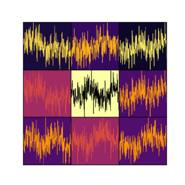
Figure 8: A qualitative visualization of the individual pixel light curves used to model the Spitzer systematics via PLD, arranged in a 3$\times$3 grid and colored according to their position and flux on the IRAC detector. Each pixel light curve is normalized such that the sum of all 9 pixels at each timestep is unity (see §5.2.1); the normalization removes astrophysical variability, enabling correlated instrumental noise to be visible on multiple timescales.

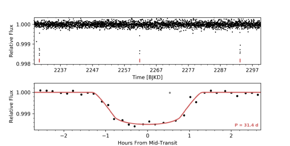
Figure 9: Top: K2 light curve produced by EVEREST 2.0 with individual transits indicated in red. Bottom: the same light curve folded on the orbital period with best-fit transit model in red. The data point in gray was identified as an outlier and ignored in the fit.

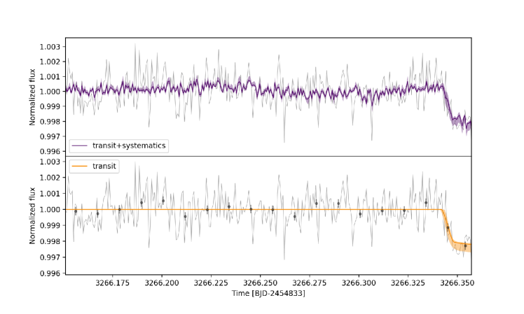
Figure 10: Top: Raw Spitzer photometry and best-fit model of the transit and systematics, with shaded 68% credible region. Bottom: Corrected light curve and best-fit transit model, with shaded 68% credible region. A partial transit of the planet was caught at the end of the observing sequence.

5.2.2 Simultaneous K2 and Spitzer analysis

We simultaneously fit the K2 and Spitzer light curves to ensure a robust recovery of the transit signal in the Spitzer data, as well as to enable the higher cadence of the Spitzer data to yield improved parameter estimates from the K2 data (Livingston et al. in review). This is achieved by sharing strictly geometric transit parameters ($a/R_{\star}$ and $b$), which are bandpass-independent, while using using separate parameters for limb-darkening, systematics, etc., which are bandpass-dependent. $R_{p}/R_{\star}$ is fit for both the Kepler and Spitzer 4.5 µm  bandpasses separately to allow for a dependence of transit depth on wavelength. Any such chromaticity is of particular interest in this case because it contains information about the levels of dilution present at each band, which in turn can determine which component of the binary is the true host of the transit signal. The K2 light curve contains only three transits, and thus only sparsely samples ingress and egress due to the 30 minute observing cadence. The impact parameter $b$ is thus poorly constrained in the fit to the K2 data alone, but the addition of the higher cadence Spitzer transit yields an improved constraint, which in turn yields a more precise measurement of $R_{p}/R_{\star}$ in the Kepler bandpass. A grazing transit geometry is strongly ruled out, and a significantly larger value of $R_{p}/R_{\star}$ is detected in the Spitzer bandpass ($\sim$3.7$\sigma$), indicating that the component of the binary that hosts the planet candidate is subject to lower levels of dilution at longer wavelengths (see Figure 11).

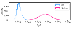
Figure 11: The marginalized posterior distributions of $R_{p}/R_{\star}$ in the K2 and Spitzer IRAC2 4.5 µm  bandpasses. $R_{p}/R_{\star}$ is significantly larger in the longer wavelength Spitzer band, indicating the component of the binary that hosts the planet is subject to lower levels of dilution at longer wavelengths

5.3 Planet Properties and Validation

We derive the planet parameters for our system assuming two configurations: the planet orbits the primary M2V and the planet orbits the secondary M3V. We complete this analysis using parameters from both our K2 and Spitzer transit fits. Results are presented in Table 3. We use Equations (4) and (6) from Furlan et al. (2017) to account for dilution in the transit for the primary and secondary scenarios, respectively. When estimating the planet radius (R_p) for our K2 derived parameters, we use the $\Delta Kep$ mag estimated in § 3.3. When estimating the planet radius from the Spitzer fit, we estimated the $\Delta IRAC2$ band magnitude using our resolved component properties and the compiled $K_{s}-W2$ colors from Pecaut & Mamajek (2013). We estimate $\Delta IRAC2$ = 0.89 $\pm$ 0.03 mag. In each case, our planet radius and equilibrium temperature estimates assume Gaussian distributed uncertainties for the parameters from Table 1 and Table 2.

We find that the K2 and Spitzer planet radii estimated assuming the candidate orbits the secondary are more consistent than when assuming it orbits the primary. This result, along with the consistency between the stellar density estimated from the transit fit ($\rho_{*}$ = $25.70^{+6.77}_{-9.39}$ g cm^-3); Table 2) and the estimated density of the M3V companion based on resolved measurements ($\rho_{*}$ = 14.2 $\pm$ 5.0  g cm^-3 ; Table 1), and the significantly deeper transit in the the Spitzer IRAC2 band, provide evidence that the candidate orbits the secondary component in the system.

Assuming the candidate transits the secondary, we applied the vespa statistical planet validation tool to the system (Morton, 2015; Montet et al., 2015). We use the stellar parameters of the secondary provided in Table 1 as input. We also include the contrast curves from our resolved NIR imaging as additional input. vespa returns a false positive probability (FPP) of 7.7 $\times$ 10^-9 when using the folded K2 transit. This FPP indicates that the transiting signal is not a bound or background eclipsing binary and we consider the transiting body a validated planet.

We conclude, using evidence provided in this section, that the observed transit is caused by a planet on a 31.39 day orbital period and most likely occurs around the secondary M3V star. We calculate the weighted mean of the K2 and Spitzer transit derived planet radii to arrive at $R_{p}$ = $1.9\pm 0.3~{}R_{\oplus}$. Given both stellar and planet parameters provided in Table 1 and Table 2 respectively, we estimate the equilibrium temperature of the planet to be roughly 226K. We adopt the following nomenclature for this system: K2-288A is the primary M2V star, K2-288B is the secondary M3V, and K2-288Bb is the planet.

6 Conclusions

We present the discovery of a small, temperate (1.9 R_⊕; 226 K) planet on a 31.39 day orbit likely around the lower-mass secondary of an M-dwarf binary system. The secondary is separated from the primary by a projected distance of $\approx$55 AU. This planetary system, K2-288, represents the third system identified by the citizen scientists of Exoplanet Explorers.

K2-288Bb is an interesting target for several reasons beyond its discovery by citizen scientists. It resides in a moderate separation low-mass binary system and likely transits the secondary. Regardless of which star in the system it orbits, its equilibrium temperature places it in or near the habitable zone and its estimated radius places it in the “Fulton gap” (Fulton et al., 2017; Fulton & Petigura, 2018; Teske et al., 2018), a likely transition zone between rocky super-Earths and volatile dominated sub-Neptunes. Thus, K2-288Bb has a radius that places it with other small planets that occur less frequently and it may still be undergoing atmospheric evolution. K2-288Bb is similar to other known planetary systems where the planet orbits one component of a multiple system, for example Kepler-296AB (Barclay et al., 2015) and Kepler-444ABC (Dupuy et al., 2016). However, this system hosts only a single detected transiting planet. Analyses of binary systems hosting transiting planets reveal that companions may have significant impacts on planet formation and evolution (Ziegler et al., 2018; Bazsó et al., 2017).

Future resolved observations of the stars could place constraints on the semi-major axis, inclination, and eccentricity of their orbit to provide further insight on the effect of the companion on system formation and evolution (e.g. Dupuy et al., 2016). This is an interesting prospect given most known M dwarf systems are compact with small planets (Gillon et al., 2017; Muirhead et al., 2015), and the K2-288 system hosts only a single planet with a relatively long (31.39 day) period. K2-288Bb is also similar to other K2 discovered small, temperate planets transiting M dwarfs, such as K2-3d, K2-18b, and K2-9b (Crossfield et al., 2015; Montet et al., 2015; Benneke et al., 2017; Schlieder et al.,, 2016) and is similar in size but significantly cooler than the well-known GJ1214b (Charbonneau et al., 2009). Transit spectroscopy of K2-288Bb with future observatories could provide insight into atmosphere evolution of similar planets of significantly different equilibrium temperatures orbiting different host stars.

With the start of science operations of the Transiting Exoplanet Survey Satellite (TESS) mission (Ricker et al., 2015), the stream of high precision photometric time series data will continue and increase in size. The role of citizen scientists will likely become even more crucial to the detection of interesting transiting exoplanets. Through continued engagement with the public via outreach and social media, we aim to foster continued interest in exoplanet citizen science and continue to validate interesting planetary systems which may otherwise be missed by automated software searches.

Table 1: Stellar Parameters

Parameter	Value	Notes
Identifying Information
K2 ID	K2-288
EPIC ID	210693462
$\alpha$ R.A. (hh:mm:ss)	03:41:46.43	EPIC
$\delta$ Dec. (dd:mm:ss)	+18:16:08.0	EPIC
$\mu_{\alpha}$ (mas yr-1)	$+186.1\pm 1.3$	UCAC5
$\mu_{\delta}$ (mas yr-1)	$-61.2\pm 1.2$	UCAC5
Barycentric RV (km s-1)	$71.6\pm 0.2$	HIRES; This Worka
Distance (pc)	69.3 $\pm$ 0.4	Gaia DR2b
Age (Myr)	$\gtrsim$ 1 Gyr	This Work
Blended Photometric Properties
$B$ (mag) ……….	$15.403\pm 0.060$	APASS DR9
$V$ (mag) ……….	$13.971\pm 0.063$	APASS DR9
$g^{\prime}$ (mag) ……….	$14.656\pm 0.016$	APASS DR9
$r^{\prime}$ (mag) ……….	$13.342\pm 0.071$	APASS DR9
$Kep$ (mag) ……….	$13.105$	EPIC
$i^{\prime}$ (mag) ……….	$12.456\pm 0.136$	APASS DR9
$J$ (mag) ……….	$10.545\pm 0.020$	2MASS
$H$ (mag) ……….	$9.946\pm 0.023$	2MASS
$K_{s}$ (mag) ………	$9.724\pm 0.018$	2MASS
$W1$ (mag) ………	$9.595\pm 0.024$	ALLWISE
$W2$ (mag) ………	$9.476\pm 0.021$	ALLWISE
$W3$ (mag) ………	$9.394\pm 0.038$	ALLWISE
$W4$ (mag) ………	$>8.750$	ALLWISE
Individual Component Propertiesc
Primary
Spectral Type ……….	M2V $\pm$ 1	This Work
$B_{p}$ (mag) ……….	$14.197\pm 0.004$	Gaia DR2
$Kep$ (mag) ……….	$13.46\pm 0.09$	This Work
$G$ (mag) ……….	$13.309\pm 0.001$	Gaia DR2
$R_{p}$ (mag) ……….	$11.982\pm 0.003$	Gaia DR2
$J$ (mag) ……….	$10.910\pm 0.027$	This Work
$H$ (mag) ……….	$10.313\pm 0.021$	This Work
$K_{s}$ (mag) ………	$10.092\pm 0.023$	This Work
$[$Fe/H$]$	$-0.29\pm 0.09$	HIRES; This Workd
$M_{*}$ ($M_{\odot}$) ……….	$0.52\pm 0.02$	This Work
$R_{*}$ ($R_{\odot}$) ……….	$0.45\pm 0.03$	This Work
$T_{eff}$ (K) ……….	$3584\pm 205$	This Work
$log(L_{*}/L_{\odot})$ ……….	$-1.49\pm 0.02$	This Work
log($g$) ……….	$4.85\pm 0.03$	This Work
$\rho$ (g cm-3) ……….	$8.1\pm 2.0$	This Work
Secondary
Spectral Type ……….	M3V $\pm$ 1	This Work
$Kep$ (mag) ……….	$14.49\pm 0.10$	This Work
$G$ (mag) ……….	$14.545\pm 0.002$	Gaia DR2
$J$ (mag) ……….	$11.907\pm 0.027$	This Work
$H$ (mag) ……….	$11.303\pm 0.021$	This Work
$K_{s}$ (mag) ………	$11.079\pm 0.023$	This Work
$[$Fe/H$]$	$-0.21\pm 0.09$	HIRES; This Workd
$M_{*}$ ($M_{\odot}$) ……….	$0.33\pm 0.02$	This Work
$R_{*}$ ($R_{\odot}$) ……….	$0.32\pm 0.03$	This Work
$T_{eff}$ (K) ……….	$3341\pm 276$	This Work
$log(L_{*}/L_{\odot})$ ……….	$-1.93\pm 0.02$	This Work
log($g$) ……….	$4.96\pm 0.02$	This Work
$\rho$ (g cm-3) ……….	$14.2\pm 5.0$	This Work

Table 2: Transit parameters.

Parameter	Unit	Value
T0-2454833	BJDTDB	$2230.402366^{+0.001162}_{-0.001107}$
P	days	$31.393463^{+0.000067}_{-0.000069}$
$a$	$R_{\star}$	$110.2^{+8.9}_{-15.5}$
b	—	$0.37^{+0.23}_{-0.25}$
i	deg.	$89.81^{+0.13}_{-0.17}$
$R_{p,K}$	$R_{\star}$	$0.0356^{+0.0012}_{-0.0010}$
$R_{p,S}$	$R_{\star}$	$0.0487^{+0.0030}_{-0.0031}$
$u_{1,K}$	—	$0.314^{+0.055}_{-0.057}$
$u_{2,K}$	—	$0.397^{+0.034}_{-0.033}$
$u_{1,S}$	—	$0.009^{+0.011}_{-0.007}$
$u_{2,S}$	—	$0.192^{+0.014}_{-0.014}$
log($\sigma_{K}$)	—	$-8.88^{+0.13}_{-0.12}$
log($\sigma_{S}$)	—	$-6.88^{+0.04}_{-0.04}$
$\rho_{\star,\mathrm{circ}}$	g cm-3	$25.70^{+6.77}_{-9.39}$
$T_{14}$	days	$0.088^{+0.003}_{-0.004}$
$T_{23}$	days	$0.079^{+0.003}_{-0.003}$
shape	—	$0.91^{+0.01}_{-0.03}$
$R_{p,\mathrm{max}}$	$R_{\star}$	$0.049^{+0.019}_{-0.006}$

Note. — The subscripts $K$ and $S$ refer to the Kepler and Spitzer 4.5 µm  bandpasses, respectively. The parameter “shape” is the ratio of $T_{23}$ to $T_{14}$, where values close to unity indicate a “box-shaped” transit caused by a small occulting body. The parameter $R_{p,max}$ corresponds to the maximum planetary radius (in units of the stellar radius) allowed by the transit geometry. log($\sigma_{K}$) and log($\sigma_{S}$) represent the width of the zero-mean Gaussian errors.

Table 3: Planet Parameters

Parameter	Unit	Value
Primary
$R_{p,K}$	$R_{\earth}$	2.06 $\pm$ 0.16
$R_{p,S}$	$R_{\earth}$	2.86 $\pm$ 0.27
$a$	AU	0.231 $\pm$ 0.03
$T_{eq}$	K	242.85$\pm$ 19.8
Secondary
$R_{p,K}$	$R_{\earth}$	1.70 $\pm$ 0.36
$R_{p,S}$	$R_{\earth}$	2.23 $\pm$ 0.47
$a$	AU	0.164 $\pm$ 0.03
$T_{eq}$	K	226.36 $\pm$ 22.3

Note. — The subscripts $K$ and $S$ refer to the Kepler and Spitzer 4.5 µm  bandpasses, respectively.

References

- Abell (1966) Abell, G. O. 1966, ApJ, 144, 259
- Aigrain et al. (2016) Aigrain, S., Parviainen, H., & Pope, B. J. S. 2016, MNRAS, 459, 2408
- Altmann et al. (2017) Altmann, M., Roeser, S., Demleitner, M., Bastian, U., & Schilbach, E. 2017, A&A, 600, L4
- Bailer-Jones et al. (2018) Bailer-Jones, C. A. L., Rybizki, J., Fouesneau, M., Mantelet, G., & Andrae, R. 2018, AJ, 156, 58
- Barclay et al. (2015) Barclay, T., Quintana, E. V., Adams, F. C., et al. 2015, ApJ, 809, 7
- Bazsó et al. (2017) Bazsó, Á., Pilat-Lohinger, E., Eggl, S., et al. 2017, MNRAS, 466, 1555
- Beichman et al. (2016) Beichman, C., Livingston, J., Werner, M., et al. 2016, ApJ, 822, 39
- Benedict et al. (2016) Benedict, G. F., Henry, T. J., Franz, O. G., et al. 2016, AJ, 152, 141
- Benneke et al. (2017) Benneke, B., Werner, M., Petigura, E., et al. 2017 ApJ, 834, 187
- Boyajian et al. (2016) Boyajian, T. S., LaCourse, D. M., Rappaport, S. A., et al. 2016, MNRAS, 457, 3988
- Burgasser et al. (2002) Burgasser, A. J., Kirkpatrick, J. D., Brown, M. E., et al. 2002, ApJ, 564, 421
- Carpenter (2001) Carpenter, J. M. 2001, AJ, 121, 2851
- Charbonneau et al. (2009) Charbonneau, D., Berta, Z. K., Irwin, J., et al. 2009, Nature, 462, 891
- Christiansen et al. (2018) Christiansen, J. L., Crossfield, I. J. M., Barenstein, G., et al. 2018, AJ, 155, 2
- Ciardi et al. (2015) Ciardi, D. R., Beichman, C. A., Horch, E. P., & Howell, S. B. 2015, ApJ, 805, 16
- Ciardi et al. (2018) Ciardi, D., Crossfield, I. J. M., Feinstein, A. D., et al. 2018, ApJ, 155, 10
- Claret et al. (2012) Claret, A., Hauschildt, P. H., Witte, S. 2012, A&A, 546, A14
- Claret et al. (2012) Claret, A., Hauschildt, P. H., & Witte, S. 2012, VizieR Online Data Catalog, 354
- Crossfield et al. (2015) Crossfield, I. J. M., Petigura, E., Schlieder, J. E., et al. 2015, ApJ, 804, 10
- Crossfield et al. (2016) Crossfield, I. J. M., Ciardi, D. R., Petigura, E. A., et al. 2016, ApJS, 226, 7
- Crossfield et al. (2018) Crossfield, I. J. M., Guerrero, N., David, T., et al. 2018, arXiv:1806.03127
- Cushing et al. (2004) Cushing, M. C., Vacca, W. D., & Rayner, J. T. 2004, PASP, 116, 362
- Cutri et al. (2003) Cutri, R. M., Skrutskie, M. F., van Dyk, S. et al. 2003, 2MASS All Sky Catalog of point sources, 2246, 0
- Cutri et al. (2014) Cutri, R. M., et al. 2014, VizieR Online Data Catalog, 2328, 0
- David et al. (2018) David, T. J., Crossfield, I. J. M., Benneke, B., et al. 2018, arXiv:1803.05056
- Deming et al. (2015) Deming, D., Knutson, H., Kammer, J., et al. 2015, ApJ, 805, 132
- Dupuy et al. (2016) Dupuy, T. J., Kratter, K. M., Kraus, A. L., et al. 2016, ApJ, 817, 80
- Dressing et al. (2017) Dressing, C. D., Newton, E. R., Schlieder, J. E., et al. 2017, ApJ, 836, 167
- Dressing et al. (2018) Dressing, C. D., Hardegree-Ullman, K., Schlieder, J. E., et al. 2018, ApJ, submitted
- Evans et al. (2018) Evans, D. W., Riello, M., De Angeli, F., et al. 2018, arXiv:1804.09368
- Fazio et al. (2004) Fazio, G. G., Hora, J. L., Allen, L. E., et al. 2004, ApJS, 154, 10
- Fischer et al. (2012) Fischer, D. A., Schwamb, M. E., Schawinski, K., et al. 2012, MNRAS, 419, 2900
- Foreman-Mackey et al. (2013) Foreman-Mackey, D., Hogg, D. W., Lang, D., & Goodman, J. 2013, PASP, 125, 306
- Fulton et al. (2017) Fulton, B. J., Petigura, E. A., Howard, A. W., et al. 2017 ApJ154, 3
- Fulton & Petigura (2018) Fulton, B. J., & Petigura, E. A. 2018, arXiv:1805.01453
- Furlan et al. (2017) Furlan, E., Ciardi, D. R., Everett, M. E., et al. 2017, AJ, 153, 71
- Gaia Collaboration et al. (2018) Gaia Collaboration, Brown, A. G. A., Vallenari, A., et al. 2018, arXiv:1804.09365
- Gies et al. (2013) Gies, D. R., Guo, Z., Howell, S. B., et al. 2013, ApJ, 775, 64
- Gillon et al. (2017) Gillon, M., Triaud, A. H. M. J.,Demory, B. O. et al. 2017, Nature, 542, 7642
- Hawley et al. (2002) Hawley, S. L., Covey, K. R., Knapp, G. R., et al. 2002, AJ, 123, 3409
- Henden et al. (2016) Henden, A. A., Templeton, M., Terrell, D., et al. 2016, VizieR Online Data Catalog, 2336
- Howard et al. (2010) Howard, A. W., Johnson, J. A., Marcy, G. W., et al. 2010, ApJ, 721, 1467
- Howell et al. (2012) Howell, S. B., Rowe, J. F., Bryson, S. T., et al. 2012, ApJ, 746, 123
- Howell et al. (2014) Howell, S. B., Sobeck, C., Haas, M., et al. 2014, PASP, 126, 398
- Huber et al. (2016) Huber, D., Bryson, S. T., Haas, M. R., et al. 2016, ApJS, 224, 2
- Kirkpatrick et al. (2000) Kirkpatrick, J. D., Reid, I. N., Liebert, J., et al. 2000, AJ, 120, 447
- Kipping (2013) Kipping, D. M. 2013, MNRAS, 435, 2152
- Knutson et al. (2012) Knutson, H. A., Lewis, N., Fortney, J. J., et al. 2012, ApJ, 754, 22
- Kolbl et al. (2015) Kolbl, R., Marcy, G. W., Isaacson, H., & Howard, A. W. 2015, AJ, 149, 18
- Kreidberg (2015) Kreidberg, L. 2015, PASP, 127, 1161
- Kreidberg (2015) Kreidberg, L. 2015, PASP, 127, 1161
- Lépine et al. (2003) Lépine, S., Rich, R. M., & Shara, M. M. 2003, AJ, 125, 3
- Lépine et al. (2013) Lépine, S., Hilton, E. J., Mann, A. W., et al. 2013, AJ, 145, 102
- Lindegren et al. (2018) Lindegren, L., Hernandez, J., Bombrun, A., et al. 2018, arXiv:1804.09366
- Lintott et al. (2008) Lintott, C. J., Schawinski, K., Slosar, A., et al. 2008, MNRAS, 389, 1179
- Luger et al. (2016) Luger, R., Agol, E., Kruse, E., et al. 2016, AJ, 152, 100
- Luger et al. (2017) Luger, R., Kruse, E., Foreman-Mackey, D., Agol, E., & Saunders, N. 2017, arXiv:1702.05488
- Mandel & Agol (2002) Mandel, K., & Agol, E. 2002, ApJ, 580, L171
- Mann et al. (2013a) Mann, A. W., Brewer, J. M., Gaidos, E., Lépine, S., & Hilton, E. J. 2013, AJ, 145, 52
- Mann et al. (2013b) Mann, A. W., Gaidos, E., Ansdell, M 2013, AJ, 779, 188
- Mann et al. (2015) Mann, A. W., Feiden, G. A., Gaidos, E., Boyajian, T., & von Braun, K. 2015, ApJ, 804, 64
- Mann et al. (2016) Mann, A. W., Feiden, G. A., Gaidos, E., Boyajian, T., & von Braun, K. 2016, ApJ, 819, 87
- Marcy et al. (2008) Marcy, G. W., Butler, R. P., Vogt, S. S., et al. 2008, Physica Scripta Volume T, 130, 014001
- Mayo et al. (2018) Mayo, A. W., Vanderburg, A., Latham, D. W., et al. 2018, AJ, 155, 136
- Montet et al. (2015) Montet, B. T., Morton, T. D., Foreman-Mackey, D., 2015, ApJ, 809, 25
- Morton (2015) Morton, T. D. 2015, Astrophysics Source Code Library, ascl:1503.011
- Muirhead et al. (2015) Muirhead, P. S., Mann, A. W., Vanderburg, A., et al. 2015, ApJ, 801, 18
- NASA Exoplanet Archive (2018) NASA Exoplanet Archive, 2018, Update 2018 February 1
- Newton et al. (2015) Newton, E. R., Charbonneau, D., Irwin, J., & Mann, A. W. 2015, ApJ, 800, 85
- Newville et al. (2014) Newville, M., Stensitzki, T., Allen, D. B., & Ingargiola, A. 2014, LMFIT: Non-Linear Least-Square Minimization and Curve-Fitting for Python¶, , , doi:10.5281/zenodo.11813. https://doi.org/10.5281/zenodo.11813
- Pecaut & Mamajek (2013) Pecaut, M. J., & Mamajek, E. E. 2013, ApJS, 208, 9
- Petigura et al. (2013a) Petigura, E. A., Marcy, G. W., & Howard, A. W. 2013, ApJ, 770, 69
- Petigura et al. (2013b) Petigura, E. A., Howard, A. W., & Marcy, G. W. 2013, Proceedings of the National Academy of Science, 110, 19273
- Petigura et al. (2015) Petigura, E. A., Schlieder, J. E., Crossfield, I. J. M., et al. 2015, ApJ, 811, 102
- Petigura et al. (2018) Petigura, E. A., Crossfield, I. J. M., Isaacson, H., et al. 2018, AJ, 155, 21
- Pont et al. (2006) Pont, F., Zucker, S., & Queloz, D. 2006, MNRAS, 373, 231
- Rayner et al. (2003) Rayner, J. T., Toomey, D. W., Onaka, P. M., et al. 2003, PASP, 115, 362
- Rayner et al. (2004) Rayner, J. T., Onaka, P. M., Cushing, M. C., & Vacca, W. D. 2004, Proc. SPIE, 5492, 1498
- Rayner et al. (2009) Rayner, J. T., Cushing, M. C., & Vacca, W. D. 2009, ApJ, 185, 289
- Ricker et al. (2015) Ricker, G. R., Winn, J. N., Vanderspek, R., et al. 2015, Journal of Astronomical Telescopes, Instruments, and Systems, 1, 014003
- Riello et al. (2018) Riello, M., De Angeli, F., Evans, D. W., et al. 2018, arXiv:1804.09367
- Rizzuto et al. (2018) Rizzuto, A. C., Vanderburg, A., Mann, A. W., et al. 2018, arXiv:1808.07068
- Rojas-Ayala et al. (2012) Rojas-Ayala, B., Covey, K. R., Muirhead, P. S., & Lloyd, J. P. 2012, ApJ, 748, 93
- Schlafly & Finkbeiner (2011) Schlafly, E. F., & Finkbeiner, D. P. 2011, ApJ, 737, 103
- Schlieder et al., (2016) Schlieder, J. E., Crossfield, I. J. M., Petigura, E. A., et al 2016, ApJ, 818, 87
- Schmitt et al. (2014) Schmitt, J. R., Agol, E., Deck, K. M., et al. 2014, ApJ, 795, 167
- Schwamb et al. (2012) Schwamb, M. E., Lintott, C. J., Fischer, D. A., et al. 2012, ApJ, 754, 129
- Teske et al. (2018) Teske, J. K., Ciardi, D. R., Howell, S. B., Hirsch, L. A., & Johnson, R. A. 2018, arXiv:1804.10170
- Vacca et al. (2003) Vacca, W. D., Cushing, M. C., & Rayner, J. T. 2003, PASP, 115, 389
- Vanderburg & Johnson (2014) Vanderburg, A., & Johnson, J. A. 2014, PASP, 126, 948
- Vogt et al. (1994) Vogt, S. S., Allen, S. L., Bigelow, B. C., et al. 1994, in Proc. SPIE, Vol. 2198, Instrumentation in Astronomy VIII, ed. D. L. Crawford & E. R. Craine, 362
- Wang et al. (2013) Wang, J., Fischer, D. A., Barclay, T., et al. 2013, ApJ, 776, 10
- Winn et al. (2008) Winn, J. N., Holman, M. J., Torres, G., et al. 2008, ApJ, 683, 1076
- Yee et al. (2017) Yee, S. W., Petigura, E. A., & von Braun, K. 2017, ApJ, 836, 77
- Yu et al. (2018) Yu, L., Crossfield, I. J. M., Schlieder, J. E., et al. 2018, arXiv:1803.04091
- Zacharias et al. (2017) Zacharias, N., Finch, C., Frouard, J., et al. 2017, AJ, 153, 4
- Ziegler et al. (2018) Ziegler, C., Law, N. M., Baranec, C., et al. 2018, arXiv:1806.10142
- Ziegler et al. (2018) Ziegler, C., Law, N. M., Baranec, C., et al. 2018, AJ, 156, 83