Fractionalized Excitations Revealed by Entanglement Entropy

Abstract

Fractionalized excitations develop in many unusual many-body states such as quantum spin liquids, disordered phases that cannot be described using any local order parameter. Because these exotic excitations correspond to emergent degrees of freedom, how to probe them and establish their existence is a long-standing challenge. We present a general procedure to reveal the fractionalized excitations using real-space entanglement entropy in critical spin liquids that are particularly relevant to experiments. Moreover, we show how to use the entanglement entropy to construct the corresponding spinon Fermi surface. Our work defines a new pathway to establish and characterize exotic excitations in novel quantum phases of matter.

Introduction — A hallmark of strongly correlated systems is the emergence of novel degrees of freedom at low energies from strong correlations. A prototype case is fractionalized excitations – fundamentally different from excitations in weakly interacting limit – such as spinons in Herbertsmithite ZnCu₃(OH)₆Cl₂ Han et al. (2011) and YbMgGaO₄ Li et al. (2015); Paddison et al. (2017); Shen et al. (2018). A particularly intriguing possibility arises in quantum spin liquids because their emergent fermionic excitations can form a Fermi surface in momentum space, rendering the properties of these insulators akin to those of conventional metals. The two-dimensional (2D) triangular lattice-based organic compounds EtMe₃Sb[Pd(dmit)₂]₂ and $\kappa$-(ET)₂Cu₂(CN)₃ Shimizu et al. (2003); Yamashita et al. (2008, 2009); Itou et al. (2010) are among the most famous candidate materials believed to host such a critical spin liquid (CSL) with an emergent spinon Fermi surface (SFS) Lee et al. (2006); Savary and Balents (2017). A four-spin ring exchange is needed to describe these materials Motrunich (2005); Block et al. (2011); He et al. (2018). An outstanding challenge is how to demonstrate and reveal the presence of fractionalized fermionic excitations, particularly with regards to the SFS.

On the theory side, it has been proposed to study the emergent SFSs in CSLs through the singular peaks in the spin structure factor (SSF) – those that arise from real-space power-law decaying spin correlations – which can be related to the locations of the SFS Lee et al. (2006). Using this procedure, recent density matrix renormalization group (DMRG) results reported the possible SFS of the spin-$1/2$ model on a triangular lattice with a four-spin ring exchange Block et al. (2011); He et al. (2018) and in the Kitaev model on a honeycomb lattice Patel and Trivedi (2019). However, it is still difficult to reconstruct the actual shape of the SFS through the DMRG results of the SSFs based on small system sizes.

An alternative quantity to describe long-range entangled states is the entanglement entropy (EE) Horodecki et al. (2009), such as the von Neumann EE and the Renyi EE (REE), which are obtained from reduced density matrix of a subsystem by tracing out the degrees of freedom outside this subsystem. The EE plays an important role in several fields, ranging from quantum information to condensed matter physics Amico et al. (2008), and has been measured experimentally Islam et al. (2015). It is believed that the EE of the ground states in most local Hamiltonians satisfies the “EE area law” Eisert et al. (2010): when a system is divided into subsystems, the EE is proportional to the area of the boundary between the two subsystems at the leading order.

Violations of the EE area law do exist in various cases. In one dimension, they are found in several quantum critical systems Calabrese and Cardy (2009). In higher dimensions, these violations are associated with the presence of a SFS in momentum space. The most well-known examples are the ground states of free fermions with Fermi surfaces Wolf (2006); Gioev and Klich (2006), where the violation is logarithmic, i.e. the EE is proportional to the surface area multiplied by a factor that grows logarithmically with the subsystem size. Intriguingly, the EE in these noninteracting systems takes the Widom formula Wolf (2006); Gioev and Klich (2006); Swingle (2010), where the coefficient of the leading term in the dependence of EE on the subsystem size captures the geometric information of the Fermi surface and that of the subsystem. For gapless electronic systems, calculations perturbative in the interactions Ding et al. (2012) show that such a violation retains the same form as that of a free Fermi gas. Recently, it has been suggested that the EE associated with the composite Fermi liquid phase of the half-filled Landau level ($\nu=1/2$) is also described by the Widom formula Mishmash and Motrunich (2016). By contrast, for frustrated strongly correlated electrons, as in Hubbard models, or spin systems, as in Heisenberg models, all with a possible emergent SFS, the EE has not been much explored Lai et al. (2013); Zhang et al. (2011).

Our present work goes beyond previous efforts and provides a generic procedure to reconstruct the geometry of the emergent SFS. We present the first variational Monte Carlo (VMC) study of the EE to test the conjectured Widom formula for strongly correlated systems. Employing a widely discussed example of a CSL with an emergent SFS, we introduce a direct probe of emergent fractionalized excitations using the real-space EE together with examining the singularity of the SSF. Remarkably, we show that the leading order of the EE has the form of the Widom formula multiplied by a previously unknown factor of $2$. This numerical factor captures the presence of two free gapless modes associated with two flavors of spinons. From this formula, we provide the basis Lai and Yang (2016) for a systematic methodology to explicitly reconstruct the emergent SFS geometry. We remark that using the SSF or EE individually only allows you to test the existence or not of fractionalized excitations (i.e. a ”yes” or ”no” answer), but a combined methodology is necessary to recover the full shape of the SFS. We also remark that we employ VMC only for simplicity: our methodology can be used if other techniques are employed, such as the quantum Monte Carlo technique or DMRG. With the only caveat that it is advisable to employ several trial states to search for self-consistency to remove the bias uncertainty intrinsic of variational procedures, our procedure is quite generic.

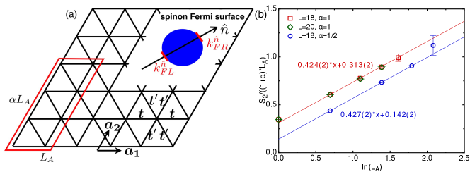
Figure 1: (a) Illustration of the subsystem geometries used to obtain the REE on the triangular lattice. In the simplest case, we consider a subsystem (illustrated in the left bottom part) consisting of $L_{A}\times\alpha L_{A}$ sites along $\bm{a}_{1}=(1,0)$ and $\bm{a}_{2}=(1/2,\sqrt{3}/2)$ directions. The top right portion illustrates the emergent SFS. For a direction $\hat{n}$, there are two Fermi patches perpendicular to $\hat{n}$ that define momenta $k^{\hat{n}}_{FR/L}$ for the right or left Fermi patches. For an emergent surface with an inversion center – natural for a system with time-reversal symmetry or inversion symmetry – the length of the difference between $\bm{k}^{\hat{n}}_{FR}$ and $\bm{k}^{\hat{n}}_{FL}$ gives its cross section along $\hat{n}$. (b) REE, $S_{2}$, for different subsystem geometries using the isotropic Gutzwiller-projected WF. Based on Eq. (1), we plot $S_{2}/((1+\alpha)L_{A})$ vs $\ln(L_{A})$. The slopes of the lines give the prefactor of the leading term of the REE. We fix the whole system size and choose the subsystem size to be $L_{A}\times\alpha L_{A}$ with $\alpha=1$ and $1/2$. The data on $L=18$ with $\alpha=1$ (red squares) are consistent with Ref. Zhang et al. (2011). We can clearly observe the proportionality $S_{2}\propto(1+\alpha)L_{A}\ln L_{A}$.

Entanglement entropy and Widom formula — We will first provide robust numerical evidence for the validity of the Widom formula in a CSL with emergent SFS. A typical ground-state wave function (WF) to represent the possible CSL on a triangular lattice Shimizu et al. (2003); Yamashita et al. (2008, 2009); Itou et al. (2010) is the Gutzwiller projected Slater determinant: $|\psi\rangle=\mathcal{P}_{G}|\psi_{0}\rangle$, where the Gutzwiller projector $\mathcal{P}_{G}=\prod_{i}(1-n_{i\uparrow}n_{i\downarrow})$ forbids double occupation on each site, and $|\psi_{0}\rangle$ is the ground state of the mean-field Hamiltonian on the triangular lattice ${\cal H}_{\rm MF}=\sum_{\langle i,j\rangle,\sigma}t_{ij}c^{{\dagger}}_{i,\sigma}c_{j,\sigma}+h.c.$. The Gutzwiller projector $\mathcal{P}_{G}$ is crucial to avoid a trivial Fermi surface of real electrons, while still allowing a possible SFS. This variational WF is known to be accurate for the quasi-1D $J_{1}-J_{2}$ spin-$1/2$ chain with four-spin exchanges Sheng et al. (2009), providing a reasonable starting point for our effort. We begin by considering an isotropic system with a total number of sites $N_{s}=L\times L$ [$t^{\prime}=t$ in Fig. 1(a)].

Based on the Widom formula, the REE associated with a subsystem consisting of $L_{A}\times\alpha L_{A}$ sites along the $\bm{a}_{1}\equiv(1,0)$ and $\bm{a}_{2}\equiv(1/2,\sqrt{3}/2)$ directions (lattice constant $a\equiv 1$), as illustrated in the bottom left portion of Fig. 1(a), can be concisely expressed as follows (derivations in Supplemental Material sup )

$$S_{2} \dot{=} \frac{c_{eff}}{8\pi}(1+\alpha)A_{sf}L_{A}\ln L_{A}$$ (1)

$$= \frac{c_{eff}}{8\pi}(1+\alpha)\left|\bm{k}^{\hat{n}}_{FR}-\bm{k}^{\hat{n}}_{FL}\right|L_{A}\ln L_{A},$$

where $\dot{=}$ means the leading logarithmic contribution in REE, $\alpha$ represents the ratio between the linear length of the subsystem ($L_{A}$) and that of the whole system ($L$), i.e. $\alpha=L_{A}/L$, and $c_{eff}$ is effectively the number of free gapless modes in the low-energy limit. Additionally, $A_{sf}$ refers to the cross section of the SFS, which is determined by the span in the momenta between right or left moving patches ($\bm{k}^{\hat{n}}_{FR/L}$) of the SFS along any particular observation direction $\hat{n}$. This is illustrated in the top right portion of Fig. 1(a), where the emergent SFS is expected to be circular.

We have carried out the VMC simulations on the triangular lattice with the whole system size fixed to be $L\times L$, with $L$ up to $20$. We calculated the REE associated with a subsystem of $L_{A}\times\alpha L_{A}$ sites, where both $L_{A}$ and $\alpha L_{A}$ are less than or equal to $L/2$. The resulting REE vs $L_{A}$ is plotted in Fig. 1(b), which shows that $S_{2}/((1+\alpha)L_{A})$ vs. $\ln L_{A}$ has the same slope for different choices of $\alpha$ within error bars. The proportionality $S_{2}\sim(1+\alpha)L_{A}\ln L_{A}$ provides direct evidence that the REE of the CSL studied here satisfies the Widom formula Eq. (1). The slope in Fig. 1(b) gives the value of the combined variable $c_{eff}A_{sf}=c_{eff}\left|\bm{k}^{\hat{n}}_{FR}-\bm{k}^{\hat{n}}_{FL}\right|$. In order to pin down the explicit formula for the REE of a CSL, additional information is needed to determine the values of $c_{eff}$ and $A_{sf}^{\hat{n}}$ separately, as addressed next.

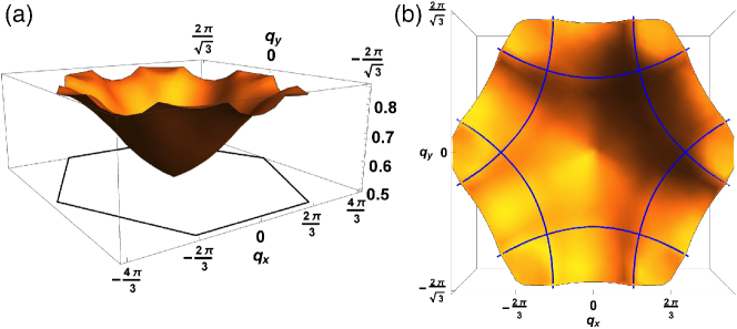
Figure 2: The 3D plot of SSF for the isotropic case. (a) Side view of the SSF within the BZ for the isotropic case (black hexagon represents the BZ), employing a triangular 30$\times$30 cluster. There is a sharp and singular peak at ${\bf q}=0$, which corresponds to the uniform real-space power-law decaying behavior. The much weaker singular lines near the boundary of the BZ correspond to the oscillating real-space behavior caused by the presence of the SFS. (b) Top view of the SSF. The blue lines are fitting results that are seen to match well with the singular lines for the SFS in the SSF on a triangular lattice consisting of $30\times 30$ sites. The details of the fitting method are in Supplemental Material sup .

Spin structure factor — Using the VMC described earlier, we calculated the SSF $D_{\bm{q}}\equiv\frac{1}{N_{s}}\sum_{i,j}\langle{\bf S}_{i}\cdot{\bf S}_{j}\rangle e^{i{\bf q}\cdot({\bf r}_{i}-{\bf r}_{j})}$ with the spin operator ${\bf S}_{i}=\sum_{\sigma,\sigma^{\prime}}{{1}\over{2}}c^{\dagger}_{i\sigma}\bm{\sigma}_{\sigma,\sigma^{\prime}}c^{\phantom{\dagger}}_{i\sigma^{\prime}}$. It is known that for an arbitrary observation direction $\hat{n}$, $D_{\bm{q}}$ should show singular peaks at $\bm{q}=\bm{0}$ and $\bm{k}^{\hat{n}}_{FR}-\bm{k}^{\hat{n}}_{FL}$, which are associated with forward and backward scattering processes. The information of $D_{\bm{q}}$ can be used to determine the cross section of the emergent SFS whose surface unit vector is perpendicular to $\hat{n}$, i.e., $A_{sf}^{\hat{n}}=\left|\bm{k}^{\hat{n}}_{FR}-\bm{k}^{\hat{n}}_{FL}\right|$ Sheng et al. (2009). In the isotropic case, $A_{sf}^{\hat{n}}=A_{sf}$ is independent of the direction.

In Fig. 2 we show the numerical data for the SSF on a triangular lattice with $30\times 30$ sites. Figure 2(a) gives a 3D side view of the SSF in the Brillouin zone (BZ), denoted by the black hexagon, where we can see a sharp singular point at $\bm{q}=0$ and weaker singular lines on the surface whose locations are theoretically suggested to be $\bm{q}=\bm{k}^{\hat{n}}_{FR}-\bm{k}^{\hat{n}}_{FL}$. Figure 2(b) shows the 3D top view of $D_{\bm{q}}$. In the present finite-size calculations, the singular lines on the 3D $D_{\bm{q}}$ surface are more clearly revealed near the BZ boundary, while the weaker singular lines inside the BZ are masked by the sharper singular point at $\bm{q}=0$. From Fig. 2(b), we can determine the location of the full singular lines by fitting $\bm{k}^{\hat{n}}_{FR}-\bm{k}^{\hat{n}}_{FL}$ Lai and Yang (2016), which allows us to extract the (average) cross sections of the emergent SFS to be $5.24\pm 0.05$. When this value for the cross section is combined with the slopes of the normalized REE vs. $\ln(L_{A})$ shown in Fig. 1(b), we obtain $c_{eff}\simeq 2.01\pm 0.02$. This value indicates the presence of two free gapless modes for each “independent” 1D patch in the low-energy limit Lee (2009), so it should be universal for all shapes of convex critical Fermi surfaces. If we introduce anisotropy into the system, $c_{eff}$ should remain the same.

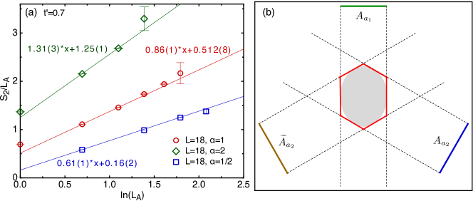
Figure 3: (a) EE in the presence of anisotropy along the zigzag bonds. We fix the whole system size to be $18\times 18$ and choose the subsystem size to be $L_{A}\times\alpha L_{A}$ with $\alpha=1/2$ (blue squares), $1$ (red circles), and $2$ (green diamonds) to extract the REE. (b) Reconstruction of the SFS with an inversion center. Based on the REE results in (a), we can obtain the cross sections of the SFS projected onto $\bm{a}_{1/2}$ axis, $A_{\bm{a}_{1/2}}$ (green and blue lines). Due to the presence of an inversion center, we can draw an inverted partner of $A_{\bm{a}_{2}}$ denoted as $\tilde{A}_{\bm{a}_{2}}$ (brown line). The dashed lines are perpendicular to $A_{\bm{a}_{1/2}}$ and $\tilde{A}_{\bm{a}_{2}}$, and connecting all the intersections of the dashed lines gives the shape of the SFS in the lowest order. The light-gray ellipse is the SFS obtained by extracting $\bm{k}^{\hat{n}}_{FR}-\bm{k}^{\hat{n}}_{FL}$ from the SSF.

Visualizing emergent spinon Fermi surface — The explicit formula for the EE obtained above can be used to reveal the emergent SFS directly. For an isotropic system, since the shape of an emergent SFS is circular, and its diameter can be extracted once the REE is calculated. To address a more general case, we focus on a triangular lattice system with anisotropy. Specifically, we consider a Gutzwiller-projected WF with hopping amplitudes $t$ along each ladder ($\pm\bm{a}_{1}$ directions) and $t^{\prime}$ along the zigzag directions ($\pm\bm{a}_{2}$ and $\pm(\bm{a}_{1}-\bm{a}_{2})$) that couple different ladders as shown at the bottom right of Fig. 1(a). For an illustration, we use $t^{\prime}/t=0.7$ to obtain the REE associated with the subsystems.

Because of numerical and computational time limitations, below we choose three subsystem geometries to obtain the REE and thereby construct the anisotropic SFS. Specifically, we calculate the REE for a subsystem with $L_{A}\times\alpha L_{A}$ sites, where we consider ratios $\alpha=1/2,~{}1,~{}2$. The REE results in these systems are shown in Fig. 3(a). Setting $c_{eff}=2$ for the present anisotropic system the formula for REE becomes:

$$S_{2}\dot{=}\frac{1}{4\pi}\left(\alpha A_{\bm{a}_{2}}+A_{\bm{a}_{1}}\right)L_{A}\ln(L_{A}),$$ (2)

where $A_{\bm{a}_{1or2}}$ represents the cross sections of the SFS projected onto the $\bm{a}_{1or2}$ axis. We can write down three equations, corresponding to $\alpha=1/2$, $1$, and $2$, respectively: (i) $A_{\bm{a}_{1}}+A_{\bm{a}_{2}}=4\pi*0.86\pm 0.01$, (ii) $A_{\bm{a}_{1}}+A_{\bm{a}_{2}}/2=4\pi*0.61\pm 0.02$, and (iii) $A_{\bm{a}_{1}}+2A_{\bm{a}_{2}}=4\pi*1.31\pm 0.03$. We can choose any two out of the three equations to obtain the values of $A_{\bm{a}_{1or2}}$. Since there are three choices, we can obtain three numerical approximations for $A_{\bm{a}_{1or2}}$, which we average over to reduce the statistical error. We find that $A_{\bm{a}_{1}}\simeq 1.53\pi$ and $A_{\bm{a}_{2}}\simeq 1.89\pi$, based on which the shape of the emergent SFS can be constructed as illustrated in Fig. 3(b). The green and the blue lines represent the cross sections of $A_{\bm{a}_{1}}$ and $A_{\bm{a}_{2}}$. Since there is an inversion center for the emergent surface in momentum space Lai and Yang (2016), once $A_{\bm{a}_{2}}$ is known, we can draw its inverted partner, denoted as $\tilde{A}_{\bm{a}_{2}}$ (brown line) in Fig. 3(b). The dashed lines are perpendicular to $A_{\bm{a}_{1/2}}$ and $\tilde{A}_{\bm{a}_{2}}$, respectively. Connecting all the intersections of the dashed lines results in the red hexagonal shape, which provides the leading-order approximation to the shape of the emergent SFS. In principle, we can improve the accuracy of the shape if we perform more (time consuming) REE calculations using different subsystem geometries Lai and Yang (2016).

For comparison, we also show the shape of the SFS in Fig. 3(b) (light-gray ellipse) obtained by extracting $\bm{k}^{\hat{n}}_{FR}-\bm{k}^{\hat{n}}_{FL}$ from the SSF. The exact numerical results for the SSF are shown in Supplemental Material. sup The emergent SFS reconstructed from the REE results is quite consistent with the light-gray ellipse in Fig. 3(b), which provides additional support for our procedure. With (costly) additional values of $\alpha$ our results will be even closer to the ellipse. We remark that in strongly correlated systems, where analytical methods are difficult to use and numerical simulations only can be performed on small clusters, it may be difficult (or sometimes impossible) to determine the locations of $\bm{k}^{\hat{n}}_{FR}-\bm{k}^{\hat{n}}_{FL}$ and thus the here proposed EE probe becomes the only practical procedure, exhibiting its unique value. From this overarching perspective, the present work builds up a foundation for using the EE to probe emergent SFSs in general cases.

Conclusion and outlook — In this work, we examined the entanglement properties of a CSL with an emergent SFS. Numerically, we have proved the validity of a generalized Widom formula Eq. (1) sup for this type of strongly correlated systems. Based on this formula, we provide a general procedure to reveal and construct the shape/size of emergent SFSs, by examining the singularity of the SSF and the real-space EE. This is an advance over previous efforts that relied on the singular peaks in the SSFs to locate the SFS by DMRG, because using only the latter the whole shape of the SFS cannot be obtained. In addition, we have obtained the universal factor $c_{eff}=2$ that describes two free gapless modes in a CSL employing robust numeral calculations, without “guessing” this value in advance.

The current work can be straightforwardly generalized to CSLs of higher-spin ($S\geq 1$) systems. Of particular interest is the 6H-B phase of $S=1$ Ba₃NiSb₂O₉ Cheng et al. (2011); Quilliam et al. (2016) that was recently suggested to realize a CSL with three flavors of fermionic spinons, forming a large SFS Fåk et al. (2017). From our perspective, it is always possible to write down a Gutzwiller-projected WF of three flavors of fermions to represent the $S=1$ CSL. Based on the results presented here, we conjecture that the leading EE in this case also satisfies the Widom formula, but with $c_{eff}=3$. Finally, our work points to new prospects for deepening the understanding of correlated systems such as heavy-fermion materials, in which the nature of quantum spins and Fermi surface plays a crucial role Si and Steglich (2010). Examining the quantum entanglement properties promises a conceptually new way of elucidating their quantum phases and criticality.

Acknowledgments. — We thank Federico Becca, Kun Yang, and Lesik Motrunich for helpful discussions. E.D. and W.-J.H. were supported by the U.S. Department of Energy (DOE), Office of Science, Basic Energy Sciences (BES), Materials Science and Engineering Division. The work was supported in part by the NSF Grant No. DMR-1920740 and the Robert A. Welch Foundation Grant No. C-1411 (W.-J.H., H.-H.L. and Q.S.), a Bethe Fellowship at Cornell University (Y.Z.), the NSF Grant No. DMR-1350237 (W.-J.H, H.-H.L. and A.H.N.), a Cottrell Scholar Award from the Research Corporation for Science Advancement, and the Robert A. Welch Foundation Grant No. C-1818 (A.H.N.), and a Smalley Postdoctoral Fellowship of the Rice Center for Quantum Materials (H.-H. L.). A.H.N. acknowledges the hospitality of the Aspen Center for Physics, which is supported by National Science Foundation Grant No. PHY-1607611. The majority of the computational calculations have been performed on the Extreme Science and Engineering Discovery Environment (XSEDE) supported by NSF under Grant No. DMR160057. Most of the numerical calculations have been done by W.-J.H. and H.-H.L. while at Rice University.

References

- Han et al. (2011) T. H. Han, J. S. Helton, S. Chu, A. Prodi, D. K. Singh, C. Mazzoli, P. Müller, D. G. Nocera, and Y. S. Lee, Phys. Rev. B 83, 100402 (2011).
- Li et al. (2015) Y. Li, H. Liao, Z. Zhang, S. Li, F. Jin, L. Ling, L. Zhang, Y. Zou, L. Pi, Z. Yang, J. Wang, Z. Wu, and Q. Zhang, Scientific reports 5, 16419 (2015).
- Paddison et al. (2017) J. A. Paddison, M. Daum, Z. Dun, G. Ehlers, Y. Liu, M. B. Stone, H. Zhou, and M. Mourigal, Nature Physics 13, 117 (2017).
- Shen et al. (2018) Y. Shen, Y.-D. Li, H. Walker, P. Steffens, M. Boehm, X. Zhang, S. Shen, H. Wo, G. Chen, and J. Zhao, Nature communications 9, 4138 (2018).
- Shimizu et al. (2003) Y. Shimizu, K. Miyagawa, K. Kanoda, M. Maesato, and G. Saito, Phys. Rev. Lett. 91, 107001 (2003).
- Yamashita et al. (2008) S. Yamashita, Y. Nakazawa, M. Oguni, Y. Oshima, H. Nojiri, Y. Shimizu, K. Miyagawa, and K. Kanoda, Nature Physics 4, 459 (2008).
- Yamashita et al. (2009) M. Yamashita, N. Nakata, Y. Kasahara, T. Sasaki, N. Yoneyama, N. Kobayashi, S. Fujimoto, T. Shibauchi, and Y. Matsuda, Nature Physics 5, 44 (2009).
- Itou et al. (2010) T. Itou, A. Oyamada, S. Maegawa, and R. Kato, Nature Physics 6, 673 (2010).
- Lee et al. (2006) P. A. Lee, N. Nagaosa, and X.-G. Wen, Rev. Mod. Phys. 78, 17 (2006).
- Savary and Balents (2017) L. Savary and L. Balents, Reports on Progress in Physics 80, 016502 (2017).
- Motrunich (2005) O. I. Motrunich, Phys. Rev. B 72, 045105 (2005).
- Block et al. (2011) M. S. Block, D. N. Sheng, O. I. Motrunich, and M. P. A. Fisher, Phys. Rev. Lett. 106, 157202 (2011).
- He et al. (2018) W.-Y. He, X. Y. Xu, G. Chen, K. T. Law, and P. A. Lee, Phys. Rev. Lett. 121, 046401 (2018).
- Patel and Trivedi (2019) N. D. Patel and N. Trivedi, Proceedings of the National Academy of Sciences 116, 12199 (2019).
- Horodecki et al. (2009) R. Horodecki, P. Horodecki, M. Horodecki, and K. Horodecki, Rev. Mod. Phys. 81, 865 (2009).
- Amico et al. (2008) L. Amico, R. Fazio, A. Osterloh, and V. Vedral, Rev. Mod. Phys. 80, 517 (2008).
- Islam et al. (2015) R. Islam, R. Ma, P. M. Preiss, M. Eric Tai, A. Lukin, M. Rispoli, and M. Greiner, Nature 528, 77 (2015).
- Eisert et al. (2010) J. Eisert, M. Cramer, and M. B. Plenio, Rev. Mod. Phys. 82, 277 (2010).
- Calabrese and Cardy (2009) P. Calabrese and J. Cardy, Journal of Physics A: Mathematical and Theoretical 42, 504005 (2009).
- Wolf (2006) M. M. Wolf, Phys. Rev. Lett. 96, 010404 (2006).
- Gioev and Klich (2006) D. Gioev and I. Klich, Phys. Rev. Lett. 96, 100503 (2006).
- Swingle (2010) B. Swingle, Phys. Rev. Lett. 105, 050502 (2010).
- Ding et al. (2012) W. Ding, A. Seidel, and K. Yang, Phys. Rev. X 2, 011012 (2012).
- Mishmash and Motrunich (2016) R. V. Mishmash and O. I. Motrunich, Phys. Rev. B 94, 081110 (2016).
- Lai et al. (2013) H.-H. Lai, K. Yang, and N. E. Bonesteel, Phys. Rev. Lett. 111, 210402 (2013).
- Zhang et al. (2011) Y. Zhang, T. Grover, and A. Vishwanath, Phys. Rev. Lett. 107, 067202 (2011).
- Lai and Yang (2016) H.-H. Lai and K. Yang, Phys. Rev. B 93, 121109 (2016).
- Sheng et al. (2009) D. N. Sheng, O. I. Motrunich, and M. P. A. Fisher, Phys. Rev. B 79, 205112 (2009).
- (29) For details of the generalized Widom formula, additional numerical results, and the fitting of the spin structure factor for the spinon Fermi surface, see Supplemental Material.
- Lee (2009) S.-S. Lee, Phys. Rev. B 80, 165102 (2009).
- Cheng et al. (2011) J. G. Cheng, G. Li, L. Balicas, J. S. Zhou, J. B. Goodenough, C. Xu, and H. D. Zhou, Phys. Rev. Lett. 107, 197204 (2011).
- Quilliam et al. (2016) J. A. Quilliam, F. Bert, A. Manseau, C. Darie, C. Guillot-Deudon, C. Payen, C. Baines, A. Amato, and P. Mendels, Phys. Rev. B 93, 214432 (2016).
- Fåk et al. (2017) B. Fåk, S. Bieri, E. Canévet, L. Messio, C. Payen, M. Viaud, C. Guillot-Deudon, C. Darie, J. Ollivier, and P. Mendels, Phys. Rev. B 95, 060402 (2017).
- Si and Steglich (2010) Q. Si and F. Steglich, Science 329, 1161 (2010).