DNS-aided explicitly filtered LES of channel flow

1 Motivation and objectives

The equations for large-eddy simulation (LES) are formally derived by applying a low-pass filter to the Navier–Stokes (NS) equations (Leonard, 1975). However, in most numerical simulations, no explicit filter form is specified, and the computational grid and the low-pass characteristics of the discrete differentiation operators act as an effective implicit filter. The resulting velocity field is then assumed to be representative of the filtered velocity. Although the discrete operators have a low-pass filtering effect, the associated filter acts only in the single spatial direction in which the derivative is applied (Lund, 2003); thus each term in the NS equations takes on a different filter form. In addition, numerical errors and the frequency content are uncontrolled for the implicit filter approach, and the solutions are grid dependent (Kravchenko & Moin, 2000; Meyers & Sagaut, 2007).

Another important limitation of implicitly filtered LES is the known fact that the subgrid scale (SGS) tensor does not coincide with the Reynolds stress terms resulting from filtering the NS equations due to the implicit filter operator. This ambiguity renders direct numerical simulation (DNS) inadequate for the development of SGS models because of inconsistent governing equations. On the contrary, when the filter operator is well defined and consistent with the filtered NS (fNS) equations, DNS data provide the necessary information to construct exact SGS models, as demonstrated by De Stefano & Vasilyev (2002) for the simple Burger’s equation. In order to exploit the rich amount of DNS data as a tool to devise SGS models, it is necessary to develop an LES framework consistent with the fNS equations, that is, explicitly filtered LES.

Previous works on explicitly filtered LES include the study of Winckelmans et al. (2001), who investigated a two-dimensional explicitly filtered isotropic turbulence and channel flow LES to evaluate various mixed subgrid/subfilter scale models. Stolz et al. (2001) implemented the three-dimensional filtering schemes of Vasilyev et al. (1998) by using an approximate deconvolution model for the convective terms in the LES equations. Lund (2003) applied two-dimensional explicit filters to a channel flow and evaluated the performance of explicitly filtered versus implicitly filtered LES. Gullbrand & Chow (2003) attempted the first grid-independent solution of the LES equations with explicit filtering. Bose et al. (2010) further investigated the grid independence of explicitly filtered LES with a three-dimensional filter for turbulent channel flows.

Nonetheless, the aforementioned investigations of wall-bounded explicitly filtered LES retain some inconsistencies with the rigorously derived incompressible fNS equations. In Lund (2003) and Gullbrand & Chow (2003), the filter operator in the wall-normal direction was implicit even though the grid resolution was too coarse to elude the use of a filter. In Vasilyev et al. (1998) and Bose et al. (2010), the filter size varied as a function of the wall-normal distance, and the divergence-free condition for incompressible flows was satisfied only up to a prescribed order of accuracy.

Recently, Bae & Lozano-Durán (2017) proposed a formulation of the incompressible fNS equations that maintain consistency between the continuity equation, the filter operator, and the boundary conditions at the wall in the continuous limit of these equations. The method utilizes an extension of the flow field across the wall, which allows the filter operator to remain constant in the wall-normal direction. Bae & Lozano-Durán (2017) performed a simulation of explicitly filtered isotropic turbulence and concluded that in absense of numerical errors, there is an one-to-one correspondence between the solutions of the NS and fNS equations. Thus, this formulation allows a direct comparison between DNS and explicitly filtered LES flow fields, which in turn can inform SGS models for explicitly filtered LES.

In this brief, we implement the formulation proposed in Bae & Lozano-Durán (2017) for an explicitly filtered LES of a plane turbulent channel flow, where the SGS model is given directly from a simultaneous simulation of DNS starting with equivalent initial conditions. The discrepancy due to numerical errors as well as truncation errors from the discretization method is observed and analyzed. This analysis can confirm whether DNS data can be used in SGS model development for explicitly filtered LES with the consistent fNS equations. The remainder of the brief is organized as follows. In Section 2, the fNS equations and the extension method for wall-bounded flows are reviewed. The numerical experiments are introduced in Section 3. The results and the error analysis are given in Section 4. Finally, conclusions are offered in Section 5.

2 Mathematical framework

2.1 Filtered Navier-Stokes equations

The incompressible NS equations and continuity condition are

$${\frac{\partial{u}_{i}}{\partial t}}+{\frac{\partial{u}_{i}{u}_{j}}{\partial x_{j}}}=-\frac{1}{\rho}{\frac{\partial{p}}{\partial x_{i}}}+\nu{\frac{\partial^{2}{u}_{i}}{\partial x_{j}\partial x_{j}}},\quad{\frac{\partial{u}_{i}}{\partial x_{i}}}=0,$$ (1)

where the velocity components are represented by ${u}_{i}$, $\rho$ is the fluid density, $\nu$ is the kinematic viscosity, and $p$ is the pressure. The filter operator on a variable $\phi$ in integral form is defined by

$$\bar{\phi}(\boldsymbol{x})\equiv\mathcal{F}(\phi)(\boldsymbol{x})=\int_{\Omega}G(t,\boldsymbol{x},\boldsymbol{x^{\prime}})\phi(\boldsymbol{x^{\prime}})\mathrm{d}\boldsymbol{x^{\prime}},$$ (2)

where $\boldsymbol{x}=(x_{1},x_{2},x_{3})$, $G$ is the filter kernel, and $\Omega$ is the domain of integration. When Eq. (1) is filtered with Eq. (2), the resulting equations are

$$\overline{\frac{\partial{u}_{i}}{\partial t}}+\overline{\frac{\partial{u}_{i}{u}_{j}}{\partial x_{j}}}=-\frac{1}{\rho}\overline{\frac{\partial{p}}{\partial x_{i}}}+\nu\overline{\frac{\partial^{2}{u}_{i}}{\partial x_{j}\partial x_{j}}},\quad\overline{\frac{\partial{u}_{i}}{\partial x_{i}}}=0.$$ (3)

The filter and differentiation operators commute when the kernel of the filter is invariant under translation in space and time; that is, $G(t,\boldsymbol{x},\boldsymbol{x^{\prime}})=G(\boldsymbol{x}-\boldsymbol{x^{\prime}})$. When this condition is satisfied, Eq. (3) can be rewritten as

$${\frac{\partial\bar{u}_{i}}{\partial t}}+{\frac{\partial\overline{{u}_{i}{u}_{j}}}{\partial x_{j}}}=-\frac{1}{\rho}{\frac{\partial\bar{p}}{\partial x_{i}}}+\nu{\frac{\partial^{2}\bar{u}_{i}}{\partial x_{j}\partial x_{j}}},\quad{\frac{\partial\bar{u}_{i}}{\partial x_{i}}}=0,$$ (4)

which is valid for both reversible ($\mathcal{F}^{-1}$ exists) and irreversible filters. For reversible filters, since no information is lost, the term $\overline{{u}_{i}{u}_{j}}$ can be expressed as a function of $\bar{u}_{i}$. For symmetric filters with Fourier transform of class $\mathcal{C}^{\infty}$, the explicit form of $\overline{{u}_{i}{u}_{j}}$ as a function of $\bar{u}_{i}$ has been extensively studied by Yeo (1987), Leonard (1997) and Carati et al. (2001), among others. In these cases, Eq. (4) can be solved independently of Eq. (1) (no closure is required), and the solution of Eq. (1), $u_{i}$, is identical to the unfiltered solution of Eq. (4), denoted by $\mathcal{F}^{-1}(\bar{u}_{i})$.

When the equations are numerically integrated, another operator is introduced, i.e., numerical discretization (e.g., the Fourier cut-off filter for spectral discretization). An in-depth analysis of the filter and discretization operators can be found in the work by Carati et al. (2001). If we denote the discretization operator by $(\tilde{\cdot})$ and assume it commutes with the differentiation operator, the discrete fNS equations become

$${\frac{\partial\tilde{\bar{u}}_{i}}{\partial t}}+{\frac{\partial\widetilde{\overline{{u}_{i}{u}_{j}}}}{\partial x_{j}}}=-\frac{1}{\rho}{\frac{\partial\tilde{\bar{p}}}{\partial x_{i}}}+\nu{\frac{\partial^{2}\tilde{\bar{u}}_{i}}{\partial x_{j}\partial x_{j}}}.$$ (5)

The convective term of Eq. (5) is usually rearranged in terms of the discrete filtered velocities, and such that

$${\frac{\partial\tilde{\bar{u}}_{i}}{\partial t}}+{\frac{\partial\widetilde{\tilde{\bar{u}}_{i}\tilde{\bar{u}}}_{j}}{\partial x_{j}}}=-\frac{1}{\rho}{\frac{\partial\tilde{\bar{p}}}{\partial x_{i}}}+\nu{\frac{\partial^{2}\tilde{\bar{u}}_{i}}{\partial x_{j}\partial x_{j}}}-\frac{\partial\widetilde{\mathcal{T}_{ij}}}{\partial x_{j}},$$ (6)

where $\mathcal{T}_{ij}=\overline{u_{i}u_{j}}-\tilde{\bar{u}}_{i}\tilde{\bar{u}}_{j}$.

The term $\mathcal{T}_{ij}$ can be further decomposed into the subfilter scale (SFS) stress tensor and the SGS stress tensor, which results from discretization errors, given that the filter and the discretization operators commute (Carati et al., 2001). However, for the remainder of the brief, we consider the combined SFS and SGS stress tensors.

One possible way of informing models for $\mathcal{T}_{ij}$ is by using DNS data. In the most extreme case, an exact SGS model can be produced for an explcitily filtered LES (Eq. 6) by running a DNS (Eq. 1) concurrently with the equivalent initial condition. By assuming that the numerical errors are negligible for the DNS velocity field, the term $\mathcal{T}_{ij}$ can be evaluated as follows:

• Using the DNS velocity field, ${u_{i}u_{j}}$ is computed.

• By filtering ${u_{i}u_{j}}$, $\overline{u_{i}u_{j}}$ is computed.

• Using the explicitly filtered LES velocity field, $\tilde{\bar{u}}_{i}\tilde{\bar{u}}_{j}$ is computed.

• $\mathcal{T}_{ij}$ is calculated by $\overline{u_{i}u_{j}}-\tilde{\bar{u}}_{i}\tilde{\bar{u}}_{j}$.

This process allows utilization of the rich DNS data available to inform SGS model development via examining the exact SGS term required for a given flow field and filter and discretization operator. Note that this would be not possible for traditional implicitly filtered LES due to the inconsistencies in the SGS terms of the LES equations and fNS equations. Methods such as machine learning or low-order approximation can later be used to form SGS models. The actual formulation of SGS models is delegated to future work. Here, we only demonstrate that DNS data can be useful for SGS model development with the consistent set of fNS equations.

2.2 Extension method

The preferred form of the fNS equations for practical applications is in Eq. (4), which requires the filter operator to commute with differentiation. This can be successfully accomplished for unbounded flows by using the same filter operator with constant filter width for the entire domain. However, the presence of a wall imposes a limitation on the support of the kernel that violates the invariance of the filter under translation in space. If $x_{2}$ is the wall-normal direction, the kernel for Eq. (2) is inevitably of the form $G(x_{2},\boldsymbol{x}-\boldsymbol{x^{\prime}})$ since the integration is bounded by the presence of the wall. Therefore, the filter and differentiation operators do not commute and Eq. (4) does not apply.

For flat walls, Bae & Lozano-Durán (2017) proposed to resolve this limitation by extending the flow in the wall-normal direction, allowing for a uniform filter in the near-wall region as illustrated in Figure 1.

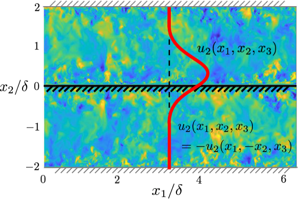
Figure 1: Illustration of the extension method in Eq. (7) for the wall-normal velocity component of a turbulent channel flow. Solid line depicts the kernel of the filter operator, which can extend beyond the wall.

Henceforth, we consider the flow over a smooth flat, wall with $x_{1},x_{2},$ and $x_{3}$ signifying the streamwise, wall-normal, and spanwise directions, respectively. Quantities evaluated at the wall, located at $x_{2}=0$, are denoted by $(\cdot)|_{w}$. The flow is then extended below the wall as

$$u_{1}(-x_{2})=u_{1}(x_{2}),\quad u_{2}(-x_{2})=-u_{2}(x_{2}),\quad u_{3}(-x_{2})=u_{3}(x_{2}),$$ (7)

where $x_{1}$ and $x_{3}$ are omitted for simplicity. In this manner, $\partial u_{i}/\partial x_{i}=0$ is also satisfied in the extended domain, preserving incompressibility. Note that the velocities in the extended domain are also consistent with the NS equations. The extension provided by Eq. (7) removes the limitation on the support of the kernel previously imposed by the wall, and Eq. (4) can be formally obtained for flows over flat walls. Note that, by symmetry, the filtered velocity field also satisfies

$$\bar{u}_{1}(-x_{2})=\bar{u}_{1}(x_{2}),\quad\bar{u}_{2}(-x_{2})=-\bar{u}_{2}(x_{2}),\quad\bar{u}_{3}(-x_{2})=\bar{u}_{3}(x_{2}).$$ (8)

Another possible extension consistent with the incompressibility condition is

$$u_{1}(-x_{2})=-u_{1}(x_{2}),\quad u_{2}(-x_{2})=u_{2}(x_{2}),\quad u_{3}(-x_{2})=-u_{3}(x_{2}).$$ (9)

However, this extension is not a compatible form, as the extended velocities do not satisfy the NS equations.

The boundary conditions for the filtered velocity field are derived by consistency with the filter operator,

$$\bar{u}_{i}|_{w}=\mathcal{F}(u_{i})|_{w}.$$ (10)

Then, the boundary conditions for the fNS equations reduce to the usual no-slip condition for the wall-normal filtered velocity and the filter-consistent boundary condition for the wall-parallel filtered velocities

$$\begin{gathered}\mathcal{F}^{-1}\left.\left(\bar{u}_{1}\right)\right|_{w}=0\text{ with }\bar{u}_{1}(-x_{2})=\bar{u}_{1}(x_{2}),\\ \bar{u}_{2}|_{w}=0,\\ \mathcal{F}^{-1}\left.\left(\bar{u}_{3}\right)\right|_{w}=0\text{ with }\bar{u}_{3}(-x_{2})=\bar{u}_{3}(x_{2}).\end{gathered}$$ (11)

This boundary condition extends to explicitly filtered LES, and the extension method can be applied to the LES equations.

3 Numerical experiment

Case	Equations	$\langle Re_{\tau}\rangle_{t}$	$\Delta_{1}^{+}$	$\Delta_{2,\min}^{+}$	$\Delta_{2,\max}^{+}$	$\Delta_{3}^{+}$
DNS	NS	$186$	8.8	1.3	19.4	8.8
LES1	fNS	$186$	8.8	1.3	19.4	8.8
LES2	fNS	$184$	17.7	2.8	38.4	17.7
LES4	fNS	$182$	35.3	5.6	76.8	35.3

Table 1: Tabulated list of cases.

We perform a set of plane turbulent channel DNS and explicitly filtered LES listed in Table 1 at friction Reynolds number $Re_{\tau}=u_{\tau}\delta/\nu\approx 180$, where $u_{\tau}$ is the friction velocity at the wall. The simulations are computed with a staggered second-order finite difference (Orlandi, 2000) and a fractional-step method (Kim & Moin, 1985) with a third-order Runge-Kutta time-advancing scheme (Wray, 1990). The code has been validated in previous studies in turbulent channel flows (Lozano-Durán & Bae, 2016; Bae et al., 2018). The size of the channel is $2\pi\delta\times 2\delta\times\pi\delta$ in the streamwise, wall-normal, and spanwise directions, respectively. Periodic boundary conditions are imposed in the streamwise and spanwise directions. The channel flow is driven by imposing a constant mean pressure gradient.

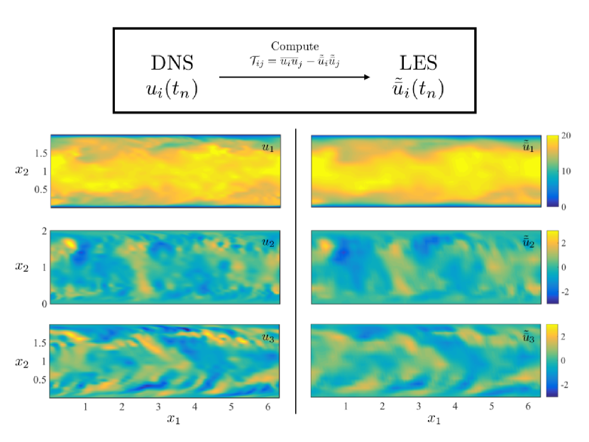
Figure 2: Schematic of how explicitly filtered LES is computed from DNS data. The term $\mathcal{T}_{ij}$ is computed at each time step from the corresponding DNS flow field and then applied to the explicitly filtered LES equations. Left panels show an instantaneous snapshot of the DNS streamwise, wall-normal and spanwise velocities, and the right panels show the corresponding instantaneous snapshot of LES1 at $t=5\delta/u_{\tau}$.

The DNS grid resolutions in the streamwise and spanwise directions are uniform with $\Delta_{1}^{+},\Delta_{3}^{+}\approx 8.8$, where the superscript $+$ denotes wall units given by $\nu$ and $u_{\tau}$. Non-uniform meshes are used in the normal direction, with the grid stretched toward the wall according to a hyperbolic tangent distribution. The height of the first grid cell at the wall is $\Delta_{2}^{+}\approx 1.3$. This grid resolution is coarser in the wall-normal direction compared with those in previous DNS cases (Kim et al., 1987), but for the purpose of our study, only the comparison between the LES and DNS cases listed here is significant. The three LES cases have grid spacings that are 1, 2 and 4 times that of the DNS. The reversible filter operator was chosen to be the differential filter (Germano, 1986)

$$G(\boldsymbol{x}-\boldsymbol{x}^{\prime};a)=\frac{1}{4\pi a^{2}}\frac{\exp(-|\boldsymbol{x}-\boldsymbol{x}^{\prime}|/a)}{|\boldsymbol{x}-\boldsymbol{x}^{\prime}|},$$ (12)

with filter parameter $a=0.1$. The parameter $a$ is related to the filter width, $\Delta_{f}$, by $a=\Delta_{f}^{2}/40$ based on an equivalent second moment with a spherical top-hat filter of radius, $\Delta_{f}/2$. The filter size was chosen to be large enough to damp the high-frequency content such that the numerical errors emanating from inaccurate high-frequency solutions of the discrete derivative operators are controlled (Carati2003).

All cases were started from an equivalent initial condition, where the initial condition of the simulations was computed by performing a preliminary simulation in DNS resolution for at least 100 eddy turnover times, defined as $\delta/u_{\tau}$. This initial condition is then filtered and interpolated to the grid resolution for each case. The interpolation, which serves as the effective discretization operator, is given by a second-order linear interpolation. Starting from the equivalent initial condition, all cases were run for $50\delta/u_{\tau}$. For the LES cases, the term $\mathcal{T}_{ij}$ is computed at each time step following the procedure given in Section 2.1 from the DNS flow field at the same time step (Figure 2). The instantaneous $u_{\tau}$ is denoted by $u_{\tau}^{\mathrm{DNS}}(t)$ and $u_{\tau}^{\mathrm{LES}}(t)$ if distinction is necessary. Time-averaged values after transients are given by $\langle\cdot\rangle_{t}$.

Note that the second-order linear interpolation discretization on a stretched mesh does not commute with the second order finite differentiation operator; thus, additional numerical commutation errors are expected. However, this is not an artifact of explicit filtering but rather the result of discretization. Higher-order interpolation methods or quadrature rules may be employed to mitigate this commutation error, and this will be investigated in future works.

4 Error assessment

Owing to the chaotic nature of turbulence, the small numerical errors that arise at each time step are expected to accumulate and affect the solution significantly for long times. Hence, we compute the associated error of LES as a function of time. The error for the instantaneous streamwise velocity field can be computed as

$$\text{error}(t)=\frac{\left[\int_{\mathcal{V}}\left(u_{1}^{\mathrm{LES}}/u_{\tau}^{\mathrm{LES}}-u_{1}^{\mathrm{DNS}}/u_{\tau}^{\mathrm{DNS}}\right)^{2}\mathrm{d}V\right]^{1/2}}{\left[\int_{\mathcal{V}}\left(u_{1}^{\mathrm{DNS}}/u_{\tau}^{\mathrm{DNS}}\right)^{2}\mathrm{d}V\right]^{1/2}},$$ (13)

where $V$ is the volume of the computational domain and $u_{i}^{\mathrm{LES}}$ is computed by reversing the differential filter on the instantaneous velocity field from the explicitly filtered LES. The error of unfiltered quantities, as opposed to the filtered ones, are examined since we are interested in predicting DNS values rather than the filtered counterparts. Figure 3 shows the error as a function of time for the three LES cases. For case LES1, where the discretization error is negligible, the error in the instantaneous velocity profile grows exponentially until it saturates at $30\delta/u_{\tau}$ (Figure 3(a)). The initial plateau for $tu_{\tau}/\delta<2$ occurs owing to the error being less than machine precision. The exponential growth of error is expected in a chaotic system with positive Lyapunov exponents, such as turbulent channel flow (Eckmann & Ruelle, 1985). The initial machine precision error between the DNS and explicitly filtered LES cases shows that the LES equations employed in this work are consistent with the NS equations and, following the argument in Section 2.1, DNS data can be useful in informing the SGS models. Cases LES2 and LES4 show a first-order growth in error that saturates around $2\delta/u_{\tau}$ (Figure 3(b)). This is possibly due to the commutation error between the interpolation (discretization) operator and the differentiation operator mentioned in Section 3.

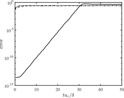
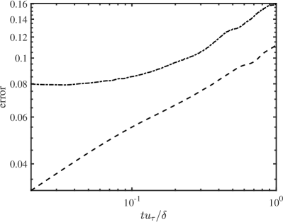
Figure 3: Error in the instantaneous velocity field as a function of time for LES1 ( ), LES2 ( ), and LES4 ( ) compared with DNS in (a) semi-log scale and (b) log-log scale (LES1 excluded).

In the remainder of the section, we study the error in the mean velocity profile and turbulence intensities for DNS-aided explicitly filtered LES.

4.1 Mean velocity profile

The error in the mean velocity profile is computed as

$$\text{error}(t)=\frac{\left[\int_{0}^{\delta}\left(\langle u_{1}^{\mathrm{LES}}/u_{\tau}^{\mathrm{LES}}\rangle-\langle u_{1}^{\mathrm{DNS}}/u_{\tau}^{\mathrm{DNS}}\rangle\right)^{2}\mathrm{d}x_{2}\right]^{1/2}}{\left[\int_{0}^{\delta}\left(\langle u_{1}^{\mathrm{DNS}}/u_{\tau}^{\mathrm{DNS}}\rangle\right)^{2}\mathrm{d}x_{2}\right]^{1/2}},$$ (14)

where $\langle\cdot\rangle$ denotes averaging in homogeneous directions. Figure 4(a) shows the error for the three LES cases as a function of time. For case LES1, the error in the mean velocity profile grows exponentially from machine precision after approximately $5\delta/u_{\tau}$ until it saturates at $30\delta/u_{\tau}$. Note that the deviation from machine precision is delayed compared with the instantaneous velocity error, indicating that the requirement of SGS models to predict the correct low-order statistics is less rigid than that for matching the instantaneous velocity fields. Since SGS models are not expected to retrieve exact instantaneous flow fields, the prediction of correct low-order statistics would be sufficient for most industrial applications. Cases LES2 and LES4 show a second-order growth in error that saturates at approximately $1\delta/u_{\tau}$.

Figure 5 shows the mean velocity profiles of the LES cases before (for LES1, $tu_{\tau}/\delta<20$; for LES2, $tu_{\tau}/\delta<1$) and after saturation of error. This shows that while the corresponding DNS flow field can be useful in forming SGS models, once the numerical errors compound and the DNS flow field ($u_{i}$ that form $\mathcal{T}_{ij}$) becomes uncorrelated to the LES flow field ($\tilde{\bar{u}}_{i}$) at the corresponding time step, it cannot provide information necessary to build effective SGS models for flow statistics.

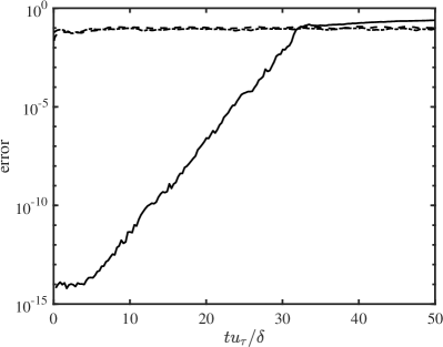
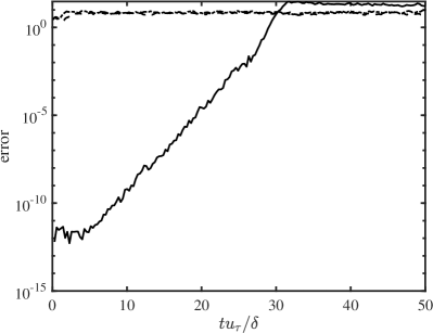
Figure 4: Error in (a) mean velocity profile and (b) streamwise turbulence intensity as a function of time for LES1 ( ), LES2 ( ), and LES4 ( ) compared with DNS.

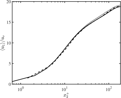
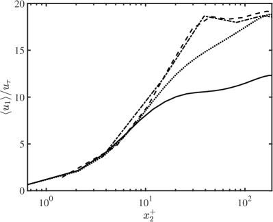
Figure 5: Mean velocity profile (a) before and (b) after saturation of error for LES1 ( ), LES2 ( ), and LES4 ( ) compared with DNS ( ).

4.2 Turbulence intensities

The error in the turbulence intensities is defined as

$$\text{error}(t)=\frac{\left[\int_{0}^{\delta}\left(\langle u_{i,\mathrm{rms}}^{\mathrm{LES}}/u_{\tau}^{\mathrm{LES}}\rangle-\langle u_{i,\mathrm{rms}}^{\mathrm{DNS}}/u_{\tau}^{\mathrm{DNS}}\rangle\right)^{2}\mathrm{d}x_{2}\right]^{1/2}}{\left[\int_{0}^{\delta}\left(\langle u_{i,\mathrm{rms}}^{\mathrm{DNS}}/u_{\tau}^{\mathrm{DNS}}\rangle\right)^{2}\mathrm{d}x_{2}\right]^{1/2}},$$ (15)

where rms denotes root-mean-squared quantities. The streamwise turbulence intensity error is depicted in Figure 4(b). Although not shown, the wall-normal and spanwise turbulence intensity errors show similar behavior. The errors in turbulence intensities are comparable to that of the mean velocity profile except for an immediate saturation of error for the LES2 and LES4 cases. This can be explained by the missing scales in the coarser LES cases, as evident from the streamwise turbulence intensity profile before saturation of error in Figure 6(a). The mismatch between the DNS profile and the profile of case LES2 before the saturation of error can be explained by the energy contained in the small scales that are present in the DNS resolution but missing in the LES2 resolution, which is expected from true LES. A fair comparison can be made by discretizing the DNS flow field to the LES resolution, effectively removing the small scales, or by taking into account the SGS contribution for the LES case. Similar to the mean velocity profile, after the saturation of error, the DNS flow field no longer is able to provide the correct SGS contribution for the LES; thus the turbulence intensity predictions diverge from the true statistics.

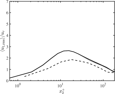
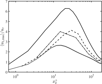
Figure 6: Streamwise turbulence intensity profile (a) before and (b) after saturation of error for LES1 ( ), LES2 ( ), and LES4 ( ) compared with DNS ( ).

5 Summary

The equations for LES are formally derived by low-pass filtering the NS equations with the effect of the small scales on the larger ones captured by a SGS model. However, it is known that the LES equations usually employed in practical applications are inconsistent with the filter operator when no explicit filter is used. Moreover, even for explicitly filtered LES, some inconsistencies remain in the wall-normal direction owing to the constraining effect of the wall. A typically undesirable effect stemming from the inconsistency between LES and the fNS equations is that DNS data cannot be used to aid SGS modeling.

Using the proposed form of the incompressible fNS equations for flows over flat walls in which the continuity equation, the filter operator, and the boundary condition at the wall are consistently formulated, we compute a set of plane turbulent channel flow explicitly filtered LES at different grid resolutions with the SGS term computed from a concurrent DNS computation starting with an equivalent initial condition. The results show that the SGS term computed from DNS provides a truthful SGS model for short times until the numerical errors compound and the two parallel computations diverge. The effective time when the statistics remain similar is longer for lower-order statistics such as mean velocity profile, as expected. This demonstrates that with the consistent fNS equations, the abundant DNS data can be used to inform SGS model development for explicitly filtered LES through methods such as machine learning. Moreover, the diverging of statistics at longer times shows that the SGS contribution computed from an uncorrelated DNS flow field is ineffective. This shows that the SGS contribution is not necessarily homogeneous as most SGS models assume, and that a more precise correlation between the instantaneous LES velocity field and the SGS model is required to capture the effect of the small scales on the resolved flow.

References

- Bae & Lozano-Durán (2017) Bae, H. J. & Lozano-Durán, A. 2017 Towards exact subgrid-scale models for explicitly filtered large-eddy simulation of wall-bounded flows. Annual Research Briefs, Center for Turbulence Research, Stanford University, pp. 207–214.
- Bae et al. (2018) Bae, H. J., Lozano-Duran, A., Bose, S. & Moin, P. 2018 Turbulence intensities in large-eddy simulation of wall-bounded flows. Phys. Rev. Fluids 3, 014610.
- Bose et al. (2010) Bose, S. T., Moin, P. & You, D. 2010 Grid-independent large-eddy simulation using explicit filtering. Phys. Fluids 22, 105103.
- Carati et al. (2001) Carati, D., Winckelmans, G. S. & Jeanmart, H. 2001 On the modelling of the subgrid-scale and filtered-scale stress tensors in large-eddy simulation. J. Fluid Mech. 441, 119–138.
- De Stefano & Vasilyev (2002) De Stefano, G. & Vasilyev, O. V. 2002 Sharp cutoff versus smooth filtering in large eddy simulation. Phys. Fluids 14, 362–369.
- Eckmann & Ruelle (1985) Eckmann, J. P. & Ruelle, D. 1985 Ergodic theory of chaos and strange attractors. In Hunt, B. R., Kennedy, J. A., Li, T.-Y. & Nusse, H. E. (Eds.) The Theory of Chaotic Attractors. Springer.
- Germano (1986) Germano, M. 1986 Differential filters for the large eddy numerical simulation of turbulent flows. Phys. Fluids 29, 1755–1757.
- Gullbrand & Chow (2003) Gullbrand, J. & Chow, F. K. 2003 The effect of numerical errors and turbulence models in large-eddy simulations of channel flow, with and without explicit filtering. J. Fluid Mech. 495, 323–341.
- Kim & Moin (1985) Kim, J. & Moin, P. 1985 Application of a fractional-step method to incompressible Navier-Stokes equations. J. Comput. Phys. 59, 308–323.
- Kim et al. (1987) Kim, J., Moin, P. & Moser, R. 1987 Turbulence statistics in fully developed channel flow at low Reynolds number. J. Fluid Mech. 177, 133–166.
- Kravchenko & Moin (2000) Kravchenko, A. G. & Moin, P. 2000 Numerical studies of flow over a circular cylinder at . Phys. Fluids 12, 403–417.
- Leonard (1975) Leonard, A. 1975 Energy cascade in large-eddy simulations of turbulent fluid flows. Adv. Geophys. 18, 237–248.
- Leonard (1997) Leonard, A. 1997 Large-eddy simulation of chaotic convection and beyond. In 35th Aerospace Sciences Meeting and Exhibit, p. 204.
- Lozano-Durán & Bae (2016) Lozano-Durán, A. & Bae, H. J. 2016 Turbulent channel with slip boundaries as a benchmark for subgrid-scale models in LES. Annual Research Briefs, Center for Turbulence Research, Stanford University, pp. 97–103.
- Lund (2003) Lund, T. S. 2003 The use of explicit filters in large eddy simulation. Comput. Math. Appl. 46, 603–616.
- Meyers & Sagaut (2007) Meyers, J. & Sagaut, P. 2007 Is plane-channel flow a friendly case for the testing of large-eddy simulation subgrid-scale models? Phys. Fluids 19, 048105.
- Orlandi (2000) Orlandi, P. 2000 Fluid Flow Phenomena: A Numerical Toolkit. Springer.
- Stolz et al. (2001) Stolz, S., Adams, N. A. & Kleiser, L. 2001 An approximate deconvolution model for large-eddy simulation with application to incompressible wall-bounded flows. Phys. Fluids 13, 997–1015.
- Vasilyev et al. (1998) Vasilyev, O. V., Lund, T. S. & Moin, P. 1998 A general class of commutative filters for LES in complex geometries. J. Comput. Phys. 146, 82–104.
- Winckelmans et al. (2001) Winckelmans, G. S., Wray, A. A., Vasilyev, O. V. & Jeanmart, H. 2001 Explicit-filtering large-eddy simulation using the tensor-diffusivity model supplemented by a dynamic Smagorinsky term. Phys. Fluids 13, 1385–1403.
- Wray (1990) Wray, A. A. 1990 Minimal-storage time advancement schemes for spectral methods. Tech. Rep. NASA Ames Research Center.
- Yeo (1987) Yeo, W. K. 1987 A generalized high pass/low pass averaging procedure for deriving and solving turbulent flow equations. PhD thesis, The Ohio State University.