Towards Autoencoding Variational Inference for Aspect-based Opinion Summary

Abstract

Aspect-based Opinion Summary (AOS), consisting of aspect discovery and sentiment classification steps, has recently been emerging as one of the most crucial data mining tasks in e-commerce systems. Along this direction, the LDA-based model is considered as a notably suitable approach, since this model offers both topic modeling and sentiment classification. However, unlike traditional topic modeling, in the context of aspect discovery it is often required some initial seed words, whose prior knowledge is not easy to be incorporated into LDA models. Moreover, LDA approaches rely on sampling methods, which need to load the whole corpus into memory, making them hardly scalable. In this research, we study an alternative approach for AOS problem, based on Autoencoding Variational Inference (AVI). Firstly, we introduce the Autoencoding Variational Inference for Aspect Discovery (AVIAD) model, which extends the previous work of Autoencoding Variational Inference for Topic Models (AVITM) to embed prior knowledge of seed words. This work includes enhancement of the previous AVI architecture and also modification of the loss function. Ultimately, we present the Autoencoding Variational Inference for Joint Sentiment/Topic (AVIJST) model. In this model, we substantially extend the AVI model to support the JST model, which performs topic modeling for corresponding sentiment. The experimental results show that our proposed models enjoy higher topic coherent, faster convergence time and better accuracy on sentiment classification, as compared to their LDA-based counterparts.

1 Introduction

Recently, Aspect-based Opinion Summary Hu  Liu (2004) has been introduced as an emerging data mining process in e-commerce systems. Generally, this task aims to extract aspects from a product review and subsequently infer the sentiments of the review writer towards the extracted aspect. The result of an AOS task is illustrated as Fig. 1. Thus, AOS consists of two major steps, known as aspect discovery and aspect-based sentiment analysis. For the first step, there are two major approaches. The first one relied on linguistic methods, such as using part-of-speech and dependency grammars analysis Qiu . (2011) or using supervised methods Jin  Ho (2009). However, this approach is likely able to detect only the explicit aspects, e.g. the aspects which are referred explicitly in the context. For example, the review such as “The price of this restaurant is quite high” can be inferred as a mention of the aspect price, explicitly discussed in the text. However, for another review of “The foods here are not very affordable”, the price aspect is also implied, but implicitly. Thus, it is hard to be detected if one only fully relies on linguistic and supervised methods. The another approach for aspect discovery is based on Latent Dirichlet Allocation (LDA) Blei . (2003), which is widely used for topic modeling Zhao . (2010). In this approach, a topic is modeled as a distribution of words in the given corpus, thus can be treated as a discovered aspect. For example, the price aspect can be discovered as a distribution over some major words such that price, expensive, affordable, cheap, etc. This approach is widely applied today to detect hidden topics in documents. For the second step of aspect-based sentiment analysis, various works based on feature-extracted machine learning are proposed, e.g. Bespalov . (2011). Recently, many works on using deep learning for sentiment classification have also been report Zhang . (2018).

However, in the context of topic discovery, perhaps the most remarkable work perhaps is the approach of Joint Sentiment/Topic model (JST) Lin  He (2009) since this work extended the usage of LDA for topic modeling as a joint system allowing not only topics to be discovered but also sentiment words associated with the topics. Thus, it is very potential to completely solve the full AOS problem using LDA-based approach, as attempted in Wu . (2015).

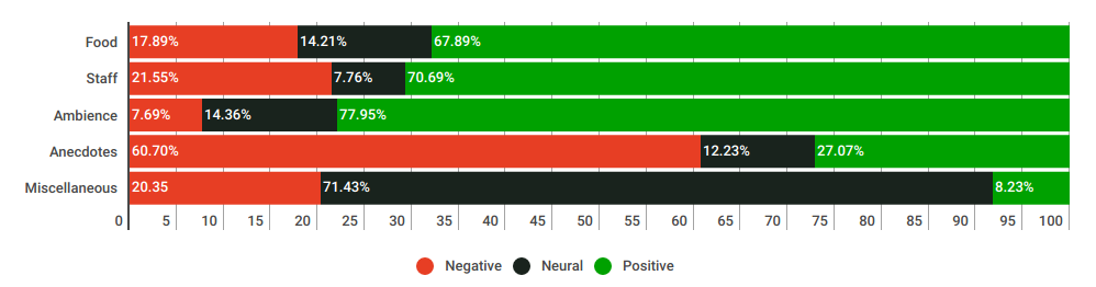
Figure 1: Aspect-based Opinion Summary result of one product.

However, aspect discovery is not entirely the same process as topic modeling. As reported in Lu . (2011), the task of aspect discovery should require some initial words for the aspects, known as the seed words. However, in LDA-based approaches, it is not easy to incorporate the prior knowledge of seed words to the topic modeling systems. Moreover, the LDA-based approaches rely on sampling methods, e.g. Gibbs sampling Blei . (2003) to learn the parameters of the required Dirichlet distributions. This work requires the whole corpus to be loaded into memory for sampling, which incurs heavy computational cost. Then, in this study, we explore the application of Autoencoding Variational Inference For Topic Models (AVITM) Srivastava  Sutton (2017) as an alternative method of LDA for AOS. In AVITM, a deep neural network is integrated in variational autoencoder Kingma  Welling (2014) with the technique of reparameterization trick to simulate the sampling work, which eventually learns the desired topic distribution as done by LDA.

Hence, the approach of AVI can achieve theoretically the same objective of hidden topic detection like LDA, but it can avoid the heavy cost of loading the whole corpus for sampling, since the input data can be gradually fed to the input layer of the deep neural network. Further, when the training data are enriched with new documents, the sampling process of LDA must be restarted from beginning, whereas in ATITM, the new documents can be incrementally trained in the neural network. Lastly, by unnormalizing the distribution of words with corresponding topics when training the neural networks, ATIVM can obtain more coherence on the generated topics.

Urged by those advantages of the AVI-based approach, we consider further extending this direction in the theme of AOS. To be concrete, we consider using AVI to support aspect discovery, not only topic modelling. In addition, we also aim to introduce an AVI-based version of the JST model, which can also perform topic modeling and sentiment classification at the same time, meanwhile still enjoying the advantages offered by AVI as aforementioned. Thus, our research contributes on the two following novel modes. The first proposal is known as Autoencoding Variational Inference for Aspect Discovery (AVIAD), in which we extend the existing work of AVITM to support incorporating prior knowledge from a set of pre-defined seed words of aspects for better discovery performance. The second model is referred to as Autoencoding Variational Inference for Joint Sentiment/Topic (AVIJST). This is our ultimate model, which can be considered as a counterpart of the JST model. However, since the autoencoders are used instead of sampling, AVIJST can easily be scalable. In addition, this model can return not only the sentiment/topic-word matrix $((S\times K)\times V)$, but also the sentiment-word matrix $(S\times V)$, which is useful in many practical situations. In addition, AVIJST can take into account the guidance from a small set of labeled data to achieve significant improvement on classification performance. The rest of the paper is organized as follows. In Section 2 we recall background knowledge of LDA and AVITM. In Section 3 and Section 4, we present the models of AVIAD and AVIJST respectively. Section 5 discusses our experimental results on some benchmark databases. Finally, Section 6 concludes the paper.

2 Latent Dirichlet Allocation and Autoencoding Variational Inference Approaches for Topic Modeling

In this section, we recall the technique of Autoencoding Variational Inference For Topic Model (AVITM) where autoencoder is adopted to play the role of Latent Dirichlet Allocation (LDA) for topic modeling.

2.1 Latent Dirichlet Allocation and Joint Sentiment/Topic model

Given a large dataset of document, or corpus, topic modeling is a unsupervised classification task that determines themes (or topics) in documents. In this context, a topic is treated as a distribution over a fixed vocabulary and a document can exhibit multiple topics (but typically not many). To fulfill this task, Latent Dirichlet Allocation (LDA) is introduced as a generative process where each document is assumed to be generated by this process. Meanwhile, Joint Sentiment-Topic (JST) model Lin  He (2009) is a generative model extended from the popular LDA model which is introduced to solve the problem of sentiment classification without prior labeled information. To generate a document, the process randomly chooses a distribution over topics. Then, each word in the document is generated by randomly choosing a topic from the distribution over topics and then randomly choosing a word from the corresponding topic.

Formally, the LDA process and JST can be visualized as graphical models given in Fig. 2a and Fig. 2b where

$\bullet$

$\beta_{1:K}$ are the topic distribution and each $\beta_{k}$ is a distribution over the vocabulary correspondingly to topic $k$;

$\bullet$

$\theta_{d}$ are the topic proportions for document $d$;

$\bullet$

$z_{d,n}$ is the topic assignment for word $n$ in document $d$;

$\bullet$

$w_{d,n}$ are the observed words for document $d$;

$\bullet$

$\alpha$ is the prior parameter of the respective Dirichlet distributions where $\theta_{d}$ is assumed.

A graphical model of JST is represented in Fig. 2b. Compared to LDA, JST has additionally the following component.

$\bullet$

$\pi_{d}$ are the sentiment proportions for document $d$;

$\bullet$

$l_{d,n}$ is the sentiment assignment for word $n$ in document $d$;

$\bullet$

$\alpha$ and $\gamma$ are the prior parameters of the respective Dirichlet distributions where $\theta_{d,s}$ and $\pi_{d}$ are assumed respectively.

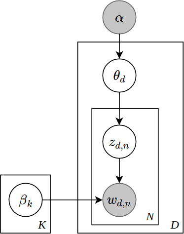
(a) LDA

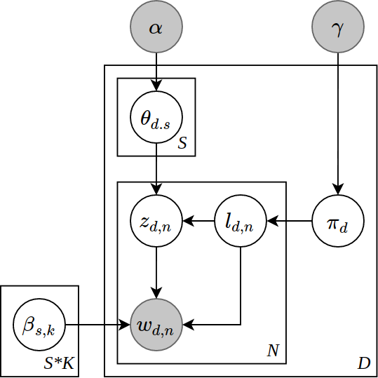
(b) JST

Figure 2: Probabilistic Graphical model of LDA and JST

Intuitively, the key idea behind the LDA process is that given a set of observed document $d$ over a vocabulary of $N$ words, we try to infer 2 sets of latent variables, which are represented by document-topic distribution and a topic-word distribution. Meanwhile, in JST, we try to infer 3 sets of latent variables, which is joint sentiment/topic-document distribution $\theta$, joint sentiment/topic-word distribution $\beta$ as well as sentiment-document distribution $\pi$ given set of observed document $d$ over a vocabulary of $N$ words.

Then, a document in the LDA process will be generated as

$$p(w|\alpha,\beta)=\int_{\theta}\left(\prod_{n=1}^{N}\sum_{z_{n}=1}^{k}p(w_{n}|z_{n},\beta)p(z_{n}|\theta)\right)p(\theta|\alpha)d\theta.$$ (1)

Meanwhile, in the JST process, each document $d$ is generated from distribution:

$$\begin{split}p(w|\alpha,\beta,\gamma)={}\int&\prod_{s}p(\theta_{s}|\alpha)\int\bigg{(}p(\pi|\gamma)\prod_{n}\sum_{s_{n}}p(s_{n}|\pi)\\ &\sum_{z_{n}}p(z_{n}|s_{n},\theta_{s})p(w_{n}|z_{n},s_{n},\beta)d{\pi}\bigg{)}d{\theta}.\end{split}$$ (2)

In LDA and JST approaches, those distributions are evaluated by sampling methods such as Gibbs sampling Lin  He (2009). However, this sampling approach required the whole corpus to be loaded into memory, which is heavily costly. Moreover, the sampling approaches prevent concurrent processing and needed to be restated when there are changes in the dataset, making this direction hardly scalable.

2.2 Variational Auto-Encoder

Autoencoder (AE) Rumelhart . (1986) is a neural network architecture which can be seen as a nonlinear function (black-box) that includes two parts: encoder and decoder, as depicted in Fig. 3.

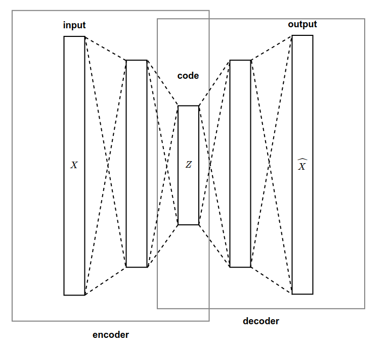
Figure 3: A general autoencoder system

Given an input $x$ in a higher-dimensional space, the encoder maps $x$ into $z$ in a lower-dimensional space as $z=f(x)$. Meanwhile, the decoder subsequently maps $z$ into $\hat{x}$ as $\hat{x}=g(z)$ where $\hat{x}$ is in the same space as $x$. The loss function of the overall network will be calculated as $\mathcal{L}(x,\hat{x})=\|x-\hat{x}\|^{2}$, whose aim is to make the decoder generate the $``same"$ input given. Once the network converges, the encoded $z$ will represent hidden features (or latent features) discovered from the input space.

However, the latent space generated by the traditional Autoencoder process is generally concrete (not continuous), thus it can well generate latent features on the samples which were previously trained. However, when generating latent information for a new sample, this method may suffer from poor performance.

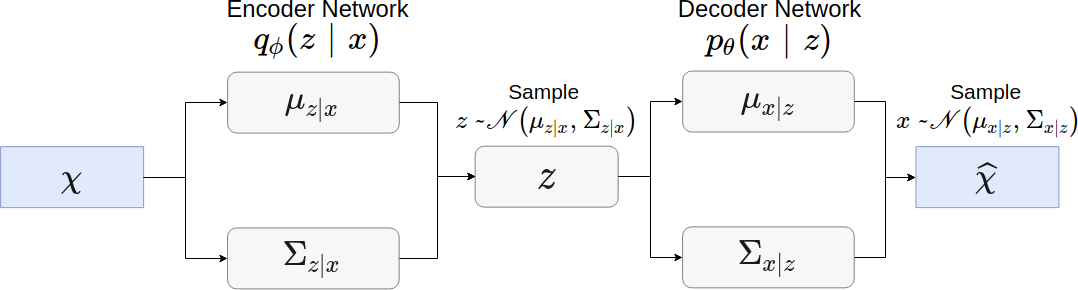
Figure 4: Variational Auto Encoder model where observable variable $x$ and its correspondent latent $z$ are distributed on Gaussian distribution $\mathcal{N}(\mu_{x|z},\Sigma_{x|z})$ and $\mathcal{N}(\mu_{z|x},\Sigma_{z|x})$, respectively.

Variational Auto-Encoder (VAE) Kingma  Welling (2014) is an extension of AE, where the latent space $z$ will be learn a posterior probability $p(z|x)$, as depicted in Fig. 4. Thus, the encoding-decoding process will be performed as follows. For an input datapoint $x_{i}$, the encoder will draw a latent variable $z$ by sampling based on the posterior probability $p(z|x)$. Then, the decoder will generate the output $\hat{x}$ by sampling based on the posterior probability $p(x|z)$. In other words, the encoder tries to learn $p(z|x)$, whereas the decoder tries to learn $p(x|z)$.

Based on Bayes theorem, $p(z|x)$ can be evaluated as

$$\centering p(z|x)=\frac{p(x|z)p(z)}{p(x)}.\@add@centering$$ (3)

However, since the prior distribution $p(x)$ is generally intractable, we will instead approximate the desired probability $p(z|x)$ by an approximated distribution $q_{\lambda}(z|x)$ where $\lambda$ is the variational parameter corresponding to the distribution family to which $q$ belongs. In VAE, $q$ is often a Gaussian distribution, hence for each data point $x_{i}$, we have $\lambda_{x_{i}}=\{\mu_{x_{i}},\sigma_{x_{i}}^{2}\}$. Moreover, VAE adopts the amortize inference Ritchie . (2016) approach, in which all of data points will share (amortize) the same $\lambda$.

Thus, the encoder part of an VAE will consists of two fully connected modules, whose roles are to respectively learn the parameter $\mu$ and $\sigma$, as presented in Fig. 4. For an input vector $x$, a latent vector $z$ will be sampled based on the currently learned value of $\mu$ and $\sigma$. The decoder will do the similar thing to reconstruct the output $\hat{x}$.

The goal of the learning process is that we try to make the variational distribution $q_{\lambda}(z|x)$ as “similar” as possible to the $p(z|x)$. To measure such similarity, one can use the Kullback-Leibler divergence Cover  Thomas (1991), which measures the information lost when using $q$ to approximate $p$:

$$\begin{split}D_{KL}(q_{\lambda}(z|x)\|p(z|x))=&\ \mathbb{E}_{q}\left[\log q_{\lambda}(z|x)\right]\\ &-\mathbb{E}_{q}[\log p(x,z)]+\log p(x).\end{split}$$ (4)

Our goal is to find the variational parameters that minimize this divergence, or $q^{*}_{\lambda}(z|x)=\arg\min_{\lambda}D_{KL}\left(q_{\lambda}(z|x)\|p(z|x)\right)$. From 4, we have

$$\text{ELBO}(\lambda)=\mathbb{E}_{q}[\log p(x,z)]-\mathbb{E}_{q}\left[\log q_{\lambda}(z|x)\right].$$ (5)

and

$$\log p(x)=\text{ELBO}(\lambda)+D_{KL}(q_{\lambda}(z|x)\|p(z|x)).$$ (6)

where ELBO stands for Evidence Lower Bound. It is due to the fact that the Kullback-Leibler divergence is always greater than or equal to zero, by Jensenfls inequality Cover  Thomas (1991). Hence, instead of minimizing the Kullback-Leibler divergence in 6, one can equally maximize $\text{ELBO}(\lambda)$.

When deployed in a VAE, $\text{ELBO}(\lambda)$ can be computed as ELBO of all data points. ELBO of a single datapoint can be expressed as

$$\text{ELBO}_{i}(\lambda)=\mathbb{E}_{q_{\lambda}(z|x_{i})}[\log p(x_{i}|z)]-D_{KL}(q_{\lambda}(z|x_{i})\|p(z)).$$ (7)

where $p(z)$ is adopted as the normal distribution $\mathcal{N}(0,1)$.

Thus, let $\theta$ and $\phi$ be the weights and biases of the encoder and decoder of the VAE, Equation 7 can be regarded as the loss function of the VAE as

$$\mathcal{L}=\underbrace{E_{q_{\phi}(z|x)}\overbrace{\left[\log p_{\theta}(x|z)\right]}^{\text{decoder}}}_{\text{reconstruction loss}}-\underbrace{D_{KL}(\overbrace{q_{\phi}(z|x)}^{\text{encoder}}\|\overbrace{p_{\theta}(z)}^{\text{prior}})}_{\text{recognition loss}}.\\$$ (8)

where the reconstruction loss measure the error occurring when the VAE reconstruct the output from the input, meanwhile the recognition loss measure the error occurring when generating the latent variable, which play the role of regularization of this loss function.

The encoder networks usually simulates Gaussian distributions, so the recognition loss has nice closed-form solution. On the other hand, the reconstruction loss can be estimated by using Monte-Carlo sampling. However, sampling method is generally indifferentiable and thus cannot be back-propagated in a NN system. Thus, in Kingma  Welling (2014), the reparameterization trick is proposed, which replaced the sampling step $z\sim p(z|x)=\mathcal{N}(\mu,\sigma^{2})$ in the training process by $z=\mu+\sigma\epsilon$ where $\epsilon$ is sampled from the trivial distribution $\mathcal{N}(0,1)$, which is differentiable.

2.3 VAE for topic modeling

From the original probability used by LDA, one can use the collapsing zfls technique Srivastava  Sutton (2017) to reduce the number of distributions that we need to compute the approximation as

$$\begin{split}p(w|\alpha,\beta)&=\int_{\theta}\left(\prod_{n=1}^{N}\sum_{z_{n}=1}^{k}p(w_{n}|z_{n},\beta)p(z_{n}|\theta)\right)p(\theta|\alpha)d\theta\\ &=\mathbb{E}_{p(\theta|\alpha)}\left[\prod_{n=1}^{N}p(w_{n}\mid\theta,\beta)\right].\end{split}$$ (9)

where $p(w|\alpha,\beta)=\text{Multinomial}\left(1,\sum_{k}\theta_{k}\beta_{k}\right)$.

Hence, one only needs to evaluate the distributions of $\theta$ and $\beta$. In Srivastava  Sutton (2017), an approach using VAE for topic modeling has been introduced to replace the old approach of LDA. VAE uses autoencoder to learn the distributions of $\theta$ and $\beta$. However, as LDA uses Dirichlet distribution, meanwhile VAE is intended to learn Gaussian distributions as previously discussed. To solve this, Laplace approximation Srivastava  Sutton (2017) is applied. Basically, a Dirichlet prior distribution $p(\theta|\alpha)$ with parameters $\alpha$ (for $K$ topics) will be approximated as $\mathcal{N}(\mu_{1},\sigma_{1})$ where $\mu_{1}$ and $\sigma_{1}$ are evaluated as below.

$$\begin{split}\mu_{1k}&=\log\alpha_{k}-\frac{1}{K}\sum_{i}^{K}{\log\alpha_{i}}.\\ \Sigma_{1kk}&=\frac{1}{\alpha_{k}}\left(1-\frac{2}{K}\right)+\frac{1}{K^{2}}\sum_{i}^{K}{\frac{1}{\alpha_{i}}}.\end{split}$$ (10)

Thus, we can compute the recognition loss by evaluating the closed-form of KL divergence between two Gaussian distributions. On the other hand, the reconstruction loss is evaluated by compute the probability density function of distribution $p(w|\alpha,\beta)=\text{Multinomial}\left(1,\sum_{k}{\theta_{k}\beta_{k}}\right)$. Therefore, the final loss function is computed as follows.

$$\begin{split}\mathcal{L}(\Theta)&=\sum_{d=1}^{D}\bigg{[}\mathbb{E}_{\epsilon\sim\mathcal{N}(0,I)}\left[w_{d}^{T}\log\left(\sigma(\beta)\sigma(\mu_{0}+\Sigma_{0}^{1/2}\epsilon)\right)\right]\\ &-\left(\frac{1}{2}\left\{tr(\Sigma_{1}^{-1}\Sigma_{0})+(\mu_{1}-\mu_{0})^{T}\Sigma_{1}^{-1}(\mu_{1}-\mu_{0})-K+\log\frac{|\Sigma_{1}|}{|\Sigma_{0}|}\right\}\right)\bigg{]}.\end{split}$$ (11)

3 Autoencoding Variational Inference for Aspect Discovery

As previously discussed, aspect discovery Chen . (2014) is a problem similar to topic modeling. Instead of discovering topics, one tries to discover aspects of concepts mentioned in a document. For example, when analyzing reviews of restaurants, the aspects that can be mentioned may include food, service, price, etc.

However, the key difference between topic modelling and aspect discovery is that the latter normally requires seed words Lu . (2011). Based on those seed words, other aspect-related terms are further discovered. In Lu . (2011), the discovery is done by incorporating seed word information via prior distribution of $\beta$ distribution into Gibbs sampling training process.

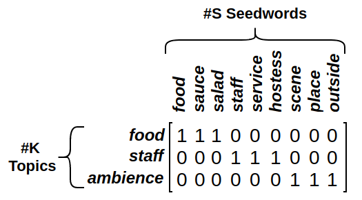
Figure 5: Prior distribution matrix.

Discovered aspects. Aspect Discovered Terms Food sauce, salad, cheese, onion, crab. Staff service, staff, rude, hostess, waiter. Ambience scene, place, wall, decorate, romantic. bold text indicates seed words.

On the other hand, in AVITM Srivastava  Sutton (2017), the authors use non-smooth version LDA illustrated in Fig. 2a, where $\beta$ has no prior distribution. Therefore, for VAE direction, we propose to modify the loss function to reflect the prior knowledge conveyed by the seed words. It is realized by our proposed Autoencoding Variational Inference for Aspect Discovery (AVIAD) model, as presented in Fig. 6.

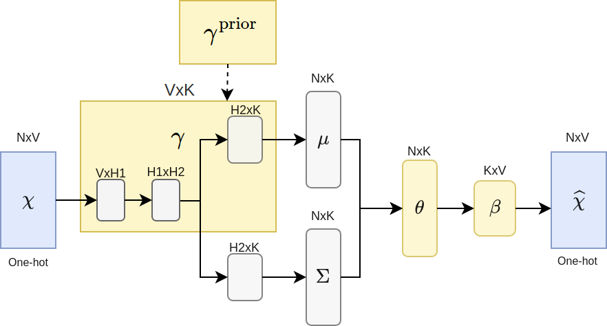
Figure 6: AutoEncoding Variational Inference for Aspect Discovery. As illustrated, the yellow block $\theta$ and $\beta$ is corresponded to the document-topic and topic-word distributions which is described in Fig. 2a, respectively. Meanwhile, $\gamma$ and $\gamma^{\text{prior}}$ are additional blocks which play an important role in the aspect discovery task.

The goal of this model is also to retrieve the topic-word distribution $\beta$, like the original model described in Sect. 2.3. However, in this model, we also embed the prior knowledge of seed words into the network structure. For example, the prior distribution $\gamma^{prior}$ of the given seed words will be represented as the matrix represented in Fig. 3

The idea behind this distribution matrix is that we want to “force”, for instance, the seed word salad to belong to the aspect Food, which is represented as the first row in the matrix. In our AVIAD model, this prior distribution $\gamma^{prior}$ is given as yellow block in Fig. 6. To incorporate this distribution in our training process, we introduce new loss function.

$$\begin{split}\mathcal{L}(\Theta)=\mathbb{E}_{q_{\phi}(\theta|w)}\left[\log p(w|\theta,\beta)\right]&-D_{KL}(q_{\phi}(\theta|w)\|p(\theta))\\ &-\lambda\sum_{n\in S}{\|\sigma(\gamma_{n})-\gamma_{n}^{prior}\|^{2}}.\end{split}$$ (12)

One can see that we have modified the ELBO in (8) by introducing the new term of (12), where each $\gamma_{n}$ is a topic distribution for each word $n$ that existed in set $S$ corresponding to document $d$. Thus, this square loss term ${||\sigma(\gamma_{n})-\gamma_{n}^{\text{prior}}||^{2}}$ will make the network try to produce the distribution $\gamma_{n}$ as similar to the prior distribution $\gamma^{\text{prior}}$ of seed words as possible. As a result, not only the predefined seed words are distributed to corresponding aspects, but also other similar words are also discovered in those aspects, as illustrated in Table 3.

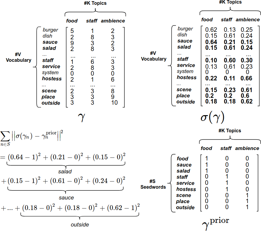
Figure 7: Example of constructing the square loss term. Firstly, every rows in the $\gamma$ matrix is normalized via softmax function. After that, a submatrix is constructed by choosing only set of words in the normalized matrix $\gamma$ such that this word must also exists in a given $\gamma^{\text{prior}}$ matrix. Finally, the prior loss is computed via the Euclidean distance between this submatrix and $\gamma^{\text{prior}}$.

For example, assume at the $k^{th}$ iteration of training process, the learning matrix $\gamma$, given as illustrated in Fig. 7, must be normalized by applying softmax function $\sigma$. Then, by minimizing the Euclidean distance between it and the prior matrix $\gamma^{\text{prior}}$ in concurrently with the other two term in Equation 12, not only the injected word such as sauce, salad, but onion, cheese will also be converged to the true aspect.

4 AutoEncoding Variational Inference for Joint Sentiment/Topic

4.1 The Proposed Model of AVIJST

In this section, we discuss our proposed ultimate model of Autoencoding Variational Inference for Aspect-based Joint Sentiment/Topic (AVIJST). Instead of training the JST model using Gibbs sampling, we want to take the advantage of Variational Autoencoder method which is fast and scalable on large dataset to this joint sentiment/topic model. First, inspired from the collapsing zfls technique Srivastava  Sutton (2017), we collapse both set of $z$ and $s$ variables . Thus, we only have to sample from $\theta$ and $\pi$ only:

$$\begin{split}p(w|\alpha,\beta,\gamma)&=\int\prod_{s}p(\theta_{s}|\alpha)\int p(\pi|\gamma)\prod_{n}p(w_{n}|\pi,\theta_{s},\beta)d{\pi}d{\theta}\\ &=\mathbb{E}_{\prod_{s}p(\theta|\alpha)p(\pi|\gamma)}\left[\prod_{s}p(w_{n}|\pi,\theta_{s},\beta)\right].\end{split}$$ (13)

where $p(w_{n}|\pi,\theta,\beta)=\text{Multinomial}\left(1,\sum_{s}{\pi_{s}\sum_{k}{\theta_{sk}\beta_{sk}}}\right)$.

In AVIJST, we no longer rely on the predefined set of seed words, since it is not easy to construct such a set with a large corpus. Instead, we observed that the distribution $\pi$ is trained through reparameterization trick to reflect the sentiment of each document, so it can be seen as a discriminant function trained in supervised model. Motivated from this, we incorporate prior knowledge by using labeled information. That is, we use a (small) set of sentiment-labeled documents to guide the learning process. In the experiment, we can also treat our model as a semi-supervised model, which needs only a small set of labeled information for classification problem. The network structure of our AVIJST is given in Fig. 8.

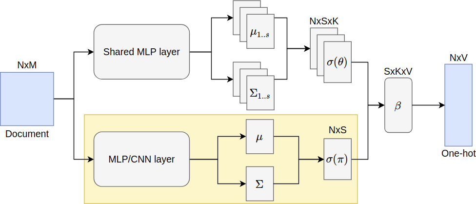
Figure 8: AutoEncoding Variational Inference for Joint Sentiment/Topic Modeling where $\theta$, $\beta$ and $\pi$ are the corresponding latent variables in JST graphical model (Fig .2b). Moreover, the yellow block which is used to mapping document $x$ to latent variable $\pi$ can be represented as any modern classification deep neural network.

In our model, the classification network for $\pi$ distribution described in the yellow block in Fig. 8, which is compatible with many kinds of neural networks. For simplicity, we only consider the Multi Layer Perceptron (MLP) network and state-of-the-art Convolution Neural Network (CNN) network combined with word embedding (WE) layer. Besides, we use the same parameters (shared network) for all $\theta_{s}$ in hidden layers of encoder network instead of constructing $s$ different encoder networks. We want to remind the readers that the soft-max layer is applied for normalization purpose at the final layer of $\sigma(\theta)$ and $\sigma(\pi)$ variables. Then, our new lower-bound function is given as

$$\begin{split}\mathcal{L}=&\underbrace{\mathbb{E}_{\prod_{s}q(\theta_{s}|w)q(\pi|w)}\left[\log\prod_{n}p(w_{n}|\pi,\theta_{s},\beta)\right]}_{\text{reconstruction loss}}+\underbrace{\mathbb{E}_{\hat{p}(\pi)}\left[-\log q(\pi|w)\right]}_{\text{classification loss}}\\ &-\underbrace{D_{KL}(q(\pi|w)\|p(\pi))-\sum_{s}D_{KL}(q(\theta_{s}|w)\|p(\theta_{s}))}_{\text{recognition loss}}.\end{split}$$ (14)

As discussed in Sect. 2.3, the reconstruction loss can be computed through Monte-Carlo sampling, while the recognition loss has nice closed-form since Laplace approximation is applied. In addition, to incorporate labeled information, we integrate the classification loss in our loss function in (14) where $\hat{p}(\pi)$ is empirical distribution.

4.2 Sentiment-word matrix

One additional advantage of our proposed AVIJST is that we can generate the sentiment-word matrix from the learning results. Firstly, we observed that each word $w$ in a document is generated by $p(w|\pi,\theta,\beta)=$ Multinomial $\left(1,\pi\theta\beta\right)$; where sentiment/topic-word distribution $\beta$ can be seen as a learning weight matrix in the decoder network which presented in Fig. 8. Inspired from this, we want our model learn another sentiment-word distribution $\nu$, which show the top word for each sentiment orientation. We integrate $\nu$ in our model by combining it linearly to generate new generative distribution:

$$p(w|\pi,\theta,\beta)=\text{Multinomial}(1,{\pi}{\theta}{\beta}+{\lambda}{\pi}{v}).$$ (15)

In Equation (15), $\lambda$ is regularization weight. In experiments section, we will illustrate some top words resulted from the constructed sentiment-word matrix.

5 Experiments

5.1 Datasets and Experimental Setup

5.1.1 Aspect Discovery

For evaluating the AVIAD model, the URSA restaurant dataset was used. It contains $2,066,324$ tokens and $52,624$ documents in total. Documents in this dataset are marked with one or more labels from the standard label set $S$ = {Food, Staff, Ambience, Price, Anecdote, Miscellaneous}. In order to avoid ambiguity, we only consider sentences with single label from three standard aspects $S$ = {Food, Staff, Ambience}. Moreover, there are two different kind of dataset will be evaluated in the experiment of topic modeling (Section 5.2) which are the imbalance and balance dataset. While only $10,000$ sentences for each aspect is evaluated in balance dataset, the imbalance dataset contains $62,348$, $23,730$ and $13,385$ sentences in Food, Staff and Ambience aspect, respectively. Finally, due to the stability of the balance dataset, it will also be used in the evaluation of supervised performance in Section 5.3.1.

We set number of topics $K=3$ corresponding to the number of chosen aspects, and Dirichlet parameter $\alpha=0.1$ in our AVIAD model. In this experiments, we compare our method with the Weak supervised LDA (WLDA) Lu . (2011), which incorporates seed word information via prior distribution of latent variable $\beta$ in LDA model. Furthermore, the set of seed words which will be fed into both models is described in Table 5.1.1.

AVIAD and WLDA seedwords. Aspect Seed words Food food sauce shrimp cheese potato fry tomato Staff staff service friendly rude hostess waiter bartender waitress Ambience atmosphere scene place table outside outdoor ambiance

5.1.2 Sentiment Classification

Regarding AVIJST model, we use two different data sets which are Large Movie Review Dataset (IMDB) and Yelp restaurant . The statistical information of these datasets are described in Table 5.1.2. Similar to the restaurant dataset, in the experiment of unsupervised performance, the sentiment datasets will also be devived into two subsets with different size, which are {10k, 25k} and {20k, 200k} for IMDB and Yelp, respectively. Moreover, due to the requirement of prior information, the subjectivity word list MPQA is also used in the re-implementation of JST model.

In the experimental setup, since we want to avoid the collapsing problem which was proposed by Srivastava  Sutton (2017), the learning rate is set very high at $0.001$ for both AVIAD and AVIJST. In addition, in AVIJST, we also set the classification learning rate to $0.005$, due to the collapsing also occurred when training the discriminant distribution $\pi$.

Statistics for IMDB and Yelp datasets. Dataset #labeled #unlabeled #testset #tokens average length IMDB 25,000 50,000 25,000 11,737,946 235 Yelp 200,000 257,156 51,432 14,799,168 58

5.2 Experimental results of topic modeling

For topic modeling performance, we compare our proposed models of AVIAD and AVIJST with their LDA-based counterparts, i.e. the Weakly supervised LDA (WLDA) Lu . (2011) and JST model with Gibbs sampling Lin  He (2009), respectively. In this experiment, we adopt the normalized point-wise mutual information (NPMI) Bouma (2009) as the main metrics to evaluate the qualitative of topic/aspects discovered by our model. The result has been proven that the set of word in discovered topic closely matches the human judgment in Lau . (2014).

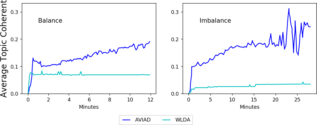
Figure 9: Aspect Discovery performance on restaurant dataset

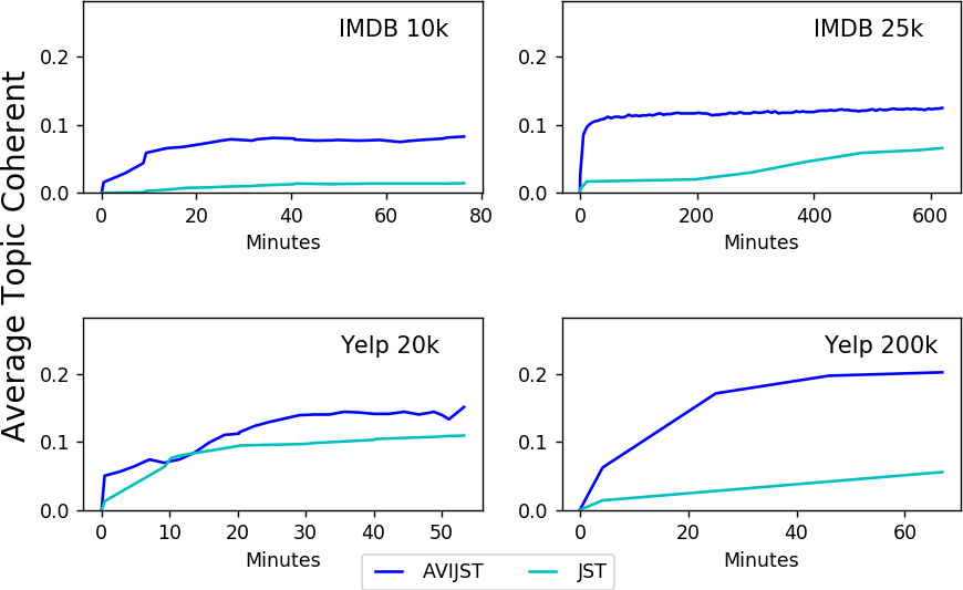
Figure 10: Joint Sentiment/Topic Modeling performance based on average topic coherent

Fig. 9 and Fig. 10 show that AVIAD and AVIJST outperforms both the traditional WLDA and JST model where the average coherent values of our proposed models converge much faster than its counterpart models. Besides, we also report the top words discovered by AVIAD and AVIJST in Table 5.2 and Table 5.2, 5.2, respectively.

Topics extracted by AVIAD and WLDA. Model Score Top words AVIAD 0.16 scallop saute shrimp broccoli spinach tuna bean 0.17 apology bill refill behavior phone busboy manage 0.28 lit chandelier banquet dimly paint wooden mirror WLDA 0.09 dish like pork good fresh taste menu 0.06 us food wait order time place even 0.10 great restaurant room nice like bar music

IMDB Topics extracted by AVIJST and JST. Positive Negative AVIJST Wrestle (0.31) Starwar (0.30) Kungfu (0 .29) Horror (0.20) War (0.22) Novel (0.27) wwe leia hong lugosi germans austen michaels ewoks cheung bela war zelah undertaker jedi kung karloff soldiers eyre hogan darth sammo dracula german rochester hulk vader tsui serum hitler novel cena soldiers shaolin undead soldier novels JST Music (0.14) Shows (0.11) Kungfu (0.21) Horror (0.13) War (0.17) Novel (0.15) music show action zombie war book musical series fight horror soldiers the dance the japanese zombies military read songs episode martial gore army novel song tv fu blood soldier books singing episodes kong dead battle adaptation

Yelp Topics extracted by AVIJST and JST. Positive Negative AVIJST Coffee (0.20) Beer (0.26) Thai food (0.36) Staff (0.16) Ambience (0.15) Japanese food (0.34) coffee beers pad rude reservation sushi latte beer thai disrespectful reservations sashimi espresso brews panang attitude waited nigiri baristas craft curry unprofessional closed rolls wifi tap kha filthy pm ayce study ipa thailand yelled phone tempura JST Coffee (0.07) Beer (0.13) Japanese food (0.20) Staff (0.08) Ambience (0.13) Thai food (0.19) coffee beer sushi staff wait thai shop bar roll rude table curry cafe selection rolls customers seated pad local beers fish people pm chicken store tap fresh customer night spicy latte pub tuna manager reservation rice

Interestingly, Table 5.2 and 5.2 shows that our AVIJST not only can extract the higher coherent topic, but also discover more specific top words for each topic than the JST model. For example, in IMDB dataset, the words “shaolin”, which is a famous styles of Chinese material arts as well as “sammo”, who is a well known actor of Chinese, are founded in topic “Kung fu”, whereas JST model only retrieved the general words like “action” and “fight”. Moreover, our AVIJST can also discover topics that JST can not find, which are “Starwar” (0.30) and “Wrestle” (0.31). Meanwhile, in Yelp dataset, due to the independent to the polarity of some common words in documents, words in topic such as Thai food and Japanese food which were founded by AVIJST are inconsistent with JST model in term of polarity. Furthermore, we also report the top words discovered for each sentiment orientation which mentioned in Sect. 4.2 in Table 5.2.

Sentiment words discovered. Datasets Polarity Sentiment words IMDB Positive excellent, wonderful, underrated, superb, flawless Negative poorly, waste, worst, pointless, awful Yelp Positive recommended, delicious, amazingly, underestimate, amicable Negative tasteless, flavorless, unimpressed, inedible, rude

5.3 Experimental results of classification performance

5.3.1 Aspect Discovery

Although AVIAD and WLDA models were first proposed as an unsupervised model, the returned $\theta$ matrix can be treated as a classification model. Therefore, the classification performance of these models are also evaluated in Table 5.3.1 via precision, recall and F1 metrics.

In general, with the same set number of seedwords, our proposed AVIAD model outperformed WLDA in most case. Regarding the staff aspect, the amount of precision which is evaluated by WLDA model (0.662) is much lower than AVIAD (0.805) due the number of food aspects sentences is significantly larger than staff. Similarly, AVIAD recall is also 10% greater than its counterpart model (0.793) on ambience aspect.

Aspect identification results. Metrics Aspect Model Precision Recall F1 Food AVIAD 0.948 0.806 0.870 WLDA 0.940 0.700 0.803 Staff AVIAD 0.805 0.887 0.842 WLDA 0.662 0.895 0.761 Ambience AVIAD 0.843 0.903 0.871 WLDA 0.844 0.793 0.817

5.3.2 Sentiment Classification

To compare with our AVIJST, we build two others neural networks. The first one is multilayer perceptron classification network with two sequential fully connected hidden layers where input is Bag-of-word models for each document, called MLP. For the second network, we construct CNN network where each document is transformed into Word Embedding vector before feeding into Convolution Neural Network layers. These two networks are integrated in our AVIJST architecture under classification network with corresponding name AVIJST-MLP and AVIJST-CNN as presented in Fig. 8. Furthermore, the model II semi supervised variational autoencoder (SSVAEII-MLP and SSVAEII-CNN) which was first proposed for semi-supervised problem in Kingma . (2014) is also evaluated in this experiment.

Accuracy on test set for IMDB. Labels Model 0 100 250 500 1k 5k 12k5 Full MLP - 68.5 77.1 80.5 82.5 84.8 86.1 87.0 CNN - 58.3 73.8 79.2 81.9 84.5 87.3 88.8 SSVAEII-MLP - 75.6 77.0 80.8 81.1 84.1 86.2 87.0 SSVAEII-CNN - 72.1 77.2 79.4 81.1 85.1 87.1 89.0 JST 57.1 - - - - - - - AVIJST-MLP - 68.2 72.7 79.9 81.2 85.9 88.2 89.7 AVIJST-CNN - 76.0 80.4 81.7 83.1 87.2 88.4 90.6

Accuracy on test set for Yelp. Labels Model 0 500 1000 Full MLP - 86.2 88.3 94.1 CNN - 85.1 87.0 94.5 SSVAEII-MLP - 87.2 87.8 94.5 SSVAEII-CNN - 84.5 86.0 94.5 JST 78.0 - - - AVIJST-MLP - 87.5 90.4 94.5 AVIJST-CNN - 88.4 89.8 94.9

Due to the lack of knowledge from MPQA prior, the supervised performance of JST model is significantly lower than others. Meanwhile, the latent variables learned by our AVIJST model outperform the solitary classification network as well as the semi supervised VAE model in most cases which is shown in Table 5.3.2 and 5.3.2. Especially, with using only 100 labeled documents over 25,000 in total on IMDB dataset, AVIJST-CNN proved that the latent variables learned in our method can help the CNN network achieve the highest accuracy (76.0 %) among them, whereas the solitary CNN showed high performance when given only a large number of labeled documents (half or full documents in the dataset in this case).

6 Conclusion

In this paper, we study using Autoencoding Variational Inference approach for Aspect-based Opinion Mining, instead of the LDA-based approaches, widely known by the Joint Sentiment/Topic model. The motivation behind is that the deep neural networks of autoencoding allow us to avoid the heavy cost of sampling, enabling this approach scalable in parallel systems. This approach also enables us to take advantages of prior knowledge from seed words or small pre-labeled guiding sets to enjoy better performance.

As a result, we introduce two models of Autoencoding Variational Inference for Aspect Discovery (AVIAD) and Autoencoding Variational Inference for Joint Sentiment /Topic (AVIJST), which outperformed their LDA-based counterparts when experimented on benchmarking datasets. Especially, the AVIJST is designed flexibly which allows any neural-network-based classification method to be integrated in an end-to-end manner. Just for example, in this work we employed MLP and the state-of-the-art CNN deep networks for classification.

Even though our AVI-based approaches have been proven outperforming the LDA-based counterparts, we have still not fully solved the AOS problem by AVI. Thus, for the future work, we aim to a complete solution by investigating a neural network architecture allowing joint distributions of aspects, documents and sentiment to be represented and trained seamlessly.

Appendix A Generative Model

In this section, we will show the generative process as well as its connection to Variational AutoEncoder in the decoder network of two aforementioned generative model LDA and JST.

A.1 LDA

Latent Dirichlet Allocation (LDA) assumes the following generative process for each document $d$ in a corpus $D$:

  for document $d$ in corpus $D$ do

     Choose $\theta_{d}\sim\text{Dirichlet}(\alpha)$

     for position $n$ in $d$ do

        Choose a topic $z_{n}\sim\text{Multinomial}(1,\theta_{d})$

        Choose a word $w_{n}\sim\text{Multinomial}(1,\beta_{z_{n}})$

     end for

  end for

Under this generative process, the marginal distribution of document $d$ is

$$p(w|\alpha,\beta)=\int_{\theta}p(\theta|\alpha)\left(\prod_{n=1}^{N}\sum_{z_{n}=1}^{K}p(w_{n}|z_{n},\beta)p(z_{n}|\theta)\right)d\theta.$$ (16)

This equation 16 can be seen as a model parameters form:

$$p(w|\alpha,\beta)=\frac{\Gamma(\sum_{i}\alpha_{i})}{\prod_{i}\Gamma(\alpha_{i})}\int_{\theta}\left(\prod_{i=1}^{K}\theta_{i}^{\alpha_{i}-1}\right)\left(\prod_{n=1}^{N}\sum_{k=1}^{K}\prod_{j=1}^{V}(\theta_{j}\beta_{kj})^{w_{n}^{j}}\right)d\theta.$$ (17)

Due to the one-hot encoding of $w_{n}^{j}$, thus, in VAE point of view, one can treat the generative distribution $p(w_{n}|\theta,\beta)$ as the decoder network.

$$p(w_{n}|\theta,\beta)=\sum_{k=1}^{K}\prod_{j=1}^{V}(\theta_{j}\beta_{kj})^{w_{n}^{j}}=\left(\theta\beta\right)^{w_{n}}.$$ (18)

where $\theta$ is the sampling matrix which is the output after using the reparameterization trick on the encoder network of $\mu_{\theta}$ and $\sigma_{\theta}$ while $\beta$ can be seen as a learning weight matrix of fully connected layer in the decoder network.

A.2 JST

A graphical model of JST is represented in Fig. 2b. Compared to LDA, JST has additionally the following component.

$\bullet$

$\pi_{d}$ are the sentiment proportions for document $d$;

$\bullet$

$l_{d,n}$ is the sentiment assignment for word $n$ in document $d$;

$\bullet$

$\alpha$ and $\gamma$ are the parameters of the respective Dirichlet distributions where $\theta_{d,s}$ and $\pi_{d}$ are assumed respectively.

Like LDA, each document $d$ is generated through a generative process

  for document $d$ in corpus $D$ do

     Choose $\pi_{d}\sim\text{Dirichlet}(\gamma)$

     for sentiment label $s$ under document $d$ do

        Choose $\theta_{d,s}\sim\text{Dirichlet}(\alpha)$

     end for

     for position $n$ in $d$ do

        Choose a sentiment $l_{n}\sim\text{Multinomial}(1,\pi_{d})$

        Choose a topic $z_{n}\sim\text{Multinomial}(1,\theta_{d,l_{n}})$

        Choose a word $w_{n}\sim\text{Multinomial}(1,\beta_{l_{n},z_{n}})$

     end for

  end for

and its correspondent marginal distribution:

$$\begin{split}p(w|\alpha,\beta,\gamma)={}\int\prod_{s}p(\theta_{s}|\alpha)\int&p(\pi|\gamma)\prod_{n}\sum_{l_{n}}p(l_{n}|\pi)\\ &\sum_{z_{n}}p(z_{n}|l_{n},\theta_{s})p(w_{n}|z_{n},l_{n},\beta)d{\pi}d{\theta}.\end{split}$$ (19)

where the reconstruction network can also be treated as a multiplication between three matrix $\theta$, $\beta$ and $\pi$.

$$p(w_{n}|\theta,\beta,\pi)=\sum_{s=1}^{S}\sum_{k=1}^{K}\prod_{j=1}^{V}(\pi_{s}\theta_{sj}\beta_{skj})^{w_{n}^{j}}=\left(\pi\theta\beta\right)^{w_{n}}.$$ (20)

References

- Bespalov \BOthers. (\APACyear2011) \APACinsertmetastarBespalov2011-ti{APACrefauthors}Bespalov, D., Bai, B., Qi, Y.\BCBL \BBA Shokoufandeh, A. \APACrefYearMonthDay2011. \BBOQ\APACrefatitleSentiment Classification Based on Supervised Latent N-gram Analysis Sentiment classification based on supervised latent n-gram analysis.\BBCQ \BIn \APACrefbtitleProceedings of the 20th ACM International Conference on Information and Knowledge Management Proceedings of the 20th acm international conference on information and knowledge management (\BPGS 375–382). \PrintBackRefs\CurrentBib
- Blei \BOthers. (\APACyear2003) \APACinsertmetastarBlei2003-dv{APACrefauthors}Blei, D\BPBIM., Ng, A\BPBIY.\BCBL \BBA Jordan, M\BPBII. \APACrefYearMonthDay2003\APACmonth03. \BBOQ\APACrefatitleLatent Dirichlet Allocation Latent dirichlet allocation.\BBCQ \APACjournalVolNumPagesJ. Mach. Learn. Res.3. \PrintBackRefs\CurrentBib
- Bouma (\APACyear2009) \APACinsertmetastarBouma-_Proceedings_of_GSCL2009-sb{APACrefauthors}Bouma, G. \APACrefYearMonthDay2009. \BBOQ\APACrefatitleNormalized (pointwise) mutual information in collocation extraction Normalized (pointwise) mutual information in collocation extraction.\BBCQ \APACjournalVolNumPagesProceedings of GSCL31–40. \PrintBackRefs\CurrentBib
- Chen \BOthers. (\APACyear2014) \APACinsertmetastarLiu-_Proceedings_of_the_52nd_annual_meeting_of_the2014-sz{APACrefauthors}Chen, Z., Mukherjee, A.\BCBL \BBA Liu, B. \APACrefYearMonthDay2014. \BBOQ\APACrefatitleAspect extraction with automated prior knowledge learning Aspect extraction with automated prior knowledge learning.\BBCQ \APACjournalVolNumPagesACL. \PrintBackRefs\CurrentBib
- Cover \BBA Thomas (\APACyear1991) \APACinsertmetastarCover:1991:EIT:129837{APACrefauthors}Cover, T\BPBIM.\BCBT \BBA Thomas, J\BPBIA. \APACrefYear1991. \APACrefbtitleElements of Information Theory Elements of information theory. \APACaddressPublisherNew York, NY, USAWiley-Interscience. \PrintBackRefs\CurrentBib
- Hu \BBA Liu (\APACyear2004) \APACinsertmetastarHu2004-sc{APACrefauthors}Hu, M.\BCBT \BBA Liu, B. \APACrefYearMonthDay2004. \BBOQ\APACrefatitleMining Opinion Features in Customer Reviews Mining opinion features in customer reviews.\BBCQ \BIn \APACrefbtitleProceedings of the 19th National Conference on Artifical Intelligence. Proceedings of the 19th national conference on artifical intelligence. \PrintBackRefs\CurrentBib
- Jin \BBA Ho (\APACyear2009) \APACinsertmetastarJin2009-wq{APACrefauthors}Jin, W.\BCBT \BBA Ho, H\BPBIH. \APACrefYearMonthDay2009. \BBOQ\APACrefatitleA Novel Lexicalized HMM-based Learning Framework for Web Opinion Mining A novel lexicalized hmm-based learning framework for web opinion mining.\BBCQ \BIn \APACrefbtitleProceedings of the 26th Annual International Conference on Machine Learning Proceedings of the 26th annual international conference on machine learning (\BPGS 465–472). \PrintBackRefs\CurrentBib
- Kingma \BOthers. (\APACyear2014) \APACinsertmetastarsemi-vae{APACrefauthors}Kingma, D\BPBIP., Rezende, D\BPBIJ., Mohamed, S.\BCBL \BBA Welling, M. \APACrefYearMonthDay2014. \BBOQ\APACrefatitleSemi-supervised Learning with Deep Generative Models Semi-supervised learning with deep generative models.\BBCQ \BIn \APACrefbtitleProceedings of the 27th International Conference on Neural Information Processing Systems - Volume 2. Proceedings of the 27th international conference on neural information processing systems - volume 2. \PrintBackRefs\CurrentBib
- Kingma \BBA Welling (\APACyear2014) \APACinsertmetastarDBLP:journals/corr/KingmaW13{APACrefauthors}Kingma, D\BPBIP.\BCBT \BBA Welling, M. \APACrefYearMonthDay2014. \BBOQ\APACrefatitleAuto-Encoding Variational Bayes Auto-encoding variational bayes.\BBCQ \APACjournalVolNumPagesICLR. \PrintBackRefs\CurrentBib
- Lau \BOthers. (\APACyear2014) \APACinsertmetastarLau2014-bx{APACrefauthors}Lau, J\BPBIH., Newman, D.\BCBL \BBA Baldwin, T. \APACrefYearMonthDay2014. \BBOQ\APACrefatitleMachine Reading Tea Leaves: Automatically Evaluating Topic Coherence and Topic Model Quality Machine reading tea leaves: Automatically evaluating topic coherence and topic model quality.\BBCQ \APACjournalVolNumPagesProceedings of the European Chapter of the Association for Computational Linguistics. \PrintBackRefs\CurrentBib
- Lin \BBA He (\APACyear2009) \APACinsertmetastarLin2009-dx{APACrefauthors}Lin, C.\BCBT \BBA He, Y. \APACrefYearMonthDay2009. \BBOQ\APACrefatitleJoint Sentiment / Topic Model for Sentiment Analysis Joint sentiment / topic model for sentiment analysis.\BBCQ \BIn \APACrefbtitleProceedings of the 18th ACM Conference on Information and Knowledge Management Proceedings of the 18th acm conference on information and knowledge management (\BPGS 375–384). \PrintBackRefs\CurrentBib
- Lu \BOthers. (\APACyear2011) \APACinsertmetastarLu2011-wh{APACrefauthors}Lu, B., Ott, M., Cardie, C.\BCBL \BBA Tsou, B\BPBIK. \APACrefYearMonthDay2011. \BBOQ\APACrefatitleMulti-aspect Sentiment Analysis with Topic Models Multi-aspect sentiment analysis with topic models.\BBCQ \BIn \APACrefbtitleProceedings of the 11th International Conference on Data Mining Workshops Proceedings of the 11th international conference on data mining workshops (\BPGS 81–88). \PrintBackRefs\CurrentBib
- Qiu \BOthers. (\APACyear2011) \APACinsertmetastarQiu2011-nu{APACrefauthors}Qiu, G., Liu, B., Bu, J.\BCBL \BBA Chen, C. \APACrefYearMonthDay2011\APACmonth03. \BBOQ\APACrefatitleOpinion Word Expansion and Target Extraction Through Double Propagation Opinion word expansion and target extraction through double propagation.\BBCQ \APACjournalVolNumPagesComput. Linguist.3719–27. \PrintBackRefs\CurrentBib
- Ritchie \BOthers. (\APACyear2016) \APACinsertmetastar2016arXiv161005735R{APACrefauthors}Ritchie, D., Horsfall, P.\BCBL \BBA Goodman, N\BPBID. \APACrefYearMonthDay2016\APACmonth10. \BBOQ\APACrefatitleDeep Amortized Inference for Probabilistic Programs Deep Amortized Inference for Probabilistic Programs.\BBCQ \APACjournalVolNumPagesArXiv e-prints. \PrintBackRefs\CurrentBib
- Rumelhart \BOthers. (\APACyear1986) \APACinsertmetastarRumelhart:1986:LIR:104279.104293{APACrefauthors}Rumelhart, D\BPBIE., Hinton, G\BPBIE.\BCBL \BBA Williams, R\BPBIJ. \APACrefYearMonthDay1986. \BBOQ\APACrefatitleParallel Distributed Processing: Explorations in the Microstructure of Cognition, Vol. 1 Parallel distributed processing: Explorations in the microstructure of cognition, vol. 1.\BBCQ \BIn D\BPBIE. Rumelhart, J\BPBIL. McClelland\BCBL \BBA C. PDP Research Group (\BEDS), (\BPGS 318–362). \APACaddressPublisherCambridge, MA, USAMIT Press. {APACrefURL} \urlhttp://dl.acm.org/citation.cfm?id=104279.104293 \PrintBackRefs\CurrentBib
- Srivastava \BBA Sutton (\APACyear2017) \APACinsertmetastar2017arXiv170301488S{APACrefauthors}Srivastava, A.\BCBT \BBA Sutton, C. \APACrefYearMonthDay2017. \BBOQ\APACrefatitleAutoencoding Variational Inference For Topic Models Autoencoding Variational Inference For Topic Models.\BBCQ \BIn \APACrefbtitleICLR. Iclr. \PrintBackRefs\CurrentBib
- Wu \BOthers. (\APACyear2015) \APACinsertmetastar2015arXiv151109128W{APACrefauthors}Wu, H., Gu, Y., Sun, S.\BCBL \BBA Gu, X. \APACrefYearMonthDay2015\APACmonth11. \BBOQ\APACrefatitleAspect-based Opinion Summarization with Convolutional Neural Networks Aspect-based Opinion Summarization with Convolutional Neural Networks.\BBCQ \APACjournalVolNumPagesArXiv e-prints. \PrintBackRefs\CurrentBib
- Zhang \BOthers. (\APACyear2018) \APACinsertmetastar2018arXiv180107883Z{APACrefauthors}Zhang, L., Wang, S.\BCBL \BBA Liu, B. \APACrefYearMonthDay2018\APACmonth01. \BBOQ\APACrefatitleDeep Learning for Sentiment Analysis : A Survey Deep Learning for Sentiment Analysis : A Survey.\BBCQ \APACjournalVolNumPagesArXiv e-prints. \PrintBackRefs\CurrentBib
- Zhao \BOthers. (\APACyear2010) \APACinsertmetastarZhao2010-bt{APACrefauthors}Zhao, W\BPBIX., Jiang, J., Yan, H.\BCBL \BBA Li, X. \APACrefYearMonthDay2010. \BBOQ\APACrefatitleJointly Modeling Aspects and Opinions with a MaxEnt-LDA Hybrid Jointly modeling aspects and opinions with a maxent-lda hybrid.\BBCQ \BIn \APACrefbtitleProceedings of the 2010 Conference on Empirical Methods in Natural Language Processing Proceedings of the 2010 conference on empirical methods in natural language processing (\BPGS 56–65). \PrintBackRefs\CurrentBib