Thick-Restart Block Lanczos Method for Large-Scale Shell-Model Calculations

Abstract

We propose a thick-restart block Lanczos method, which is an extension of the thick-restart Lanczos method with the block algorithm, as an eigensolver of the large-scale shell-model calculations. This method has two advantages over the conventional Lanczos method: the precise computations of the near-degenerate eigenvalues, and the efficient computations for obtaining a large number of eigenvalues. These features are quite advantageous to compute highly excited states where the eigenvalue density is rather high. A shell-model code, named KSHELL, equipped with this method was developed for massively parallel computations, and it enables us to reveal nuclear statistical properties which are intensively investigated by recent experimental facilities. We describe the algorithm and performance of the KSHELL code and demonstrate that the present method outperforms the conventional Lanczos method.

I Introduction

Solving a quantum many-body problem having protons and neutrons as constituent particles is one of the ultimate goals in nuclear structure physics. Although nucleons do not have an external field like electrons in an atom, nuclear shell model is successful in describing the low-lying excitation spectra of nuclei near closed-shell nuclei mayerjensen . Based on the success of the nuclear shell model, large-scale shell-model (LSSM) calculations have been performed to go far beyond closed-shell nuclei. In the LSSM, we assume that a nucleus is composed of an inert core and active particles that move in some active orbitals. The active particles and active orbitals are usually taken as valence particles and the orbitals in the valence shell, respectively. The nuclear wave function is expressed as a superposition of the Slater determinants, which represent occupations of the active particles in the orbitals. The LSSM is also called configuration interaction calculations like in quantum chemistry. By utilizing the LSSM, low-energy nuclear spectroscopic data of $sd$-shell usd ; usdab and $pf$-shell gxpf1a ; jun45 nuclei have been investigated systematically. Recent progress in radioactive ion beam facilities enables us to reveal exotic nuclear structures of unstable nuclei otsuka-review ; caurier_rmp .

In shell-model calculations we solve the Schrödinger equation of protons and neutrons as an eigenvalue problem of a huge sparse real symmetric matrix utilizing the traditional methods: the Lanczos method lanczos and the thick-restart Lanczos method tr-lanczos . These methods are known to be quite effective to obtain a small number of the lowest eigenvalues of a sparse matrix. Moreover, several efforts have been paid to pursue a better eigensolver, such as the Sakurai-Sugiura method mizusaki-ss ; ss-method and the Locally Optimal Block Preconditioned Conjugate Gradient method mfdn-lobpcg .

In many cases, a small number of low-lying eigenvalues and eigenvectors need to be calculated by the LSSM calculations, since in many experimental studies of unstable nuclei only a small number of low-lying states can be measured. In order to analyze such low-lying states, more than a dozen shell-model codes had been developed antoine ; bigstick ; eicode ; kshell ; nathan ; nushell ; nushellx ; MFDn ; mshell ; mshell64 ; oxbash ; vecsse . However, recent progress of the experimental techniques extends the opportunity to investigate highly excited states and their statistic properties, such as $\gamma$-ray strength functions and level densities oslo . In order to discuss these properties by shell-model calculations precisely, a relatively large number of eigenstates ($O(10^{2})$-$O(10^{3})$) are required by solving the eigenvalue problem La133-palit ; sieja-leh ; jorgen-m1 ; ld-ni58 . In the present paper, we propose the thick-restart block Lanczos method to compute these states efficiently, and describe the implementation and the performance of the KSHELL code which we developed kshell . In the code we adopt an algorithm of generating the matrix elements on the fly in order to avoid storing the matrix elements and to save memory usage, while the generation of the matrix elements costs a certain amount of the computation time. We will also demonstrate the block method reduces this cost in the present paper.

The thick-restart block Lanczos method is a combination of the block Lanczos method and the thick-restart method. The block Lanczos method was proposed as a general eigenvalue solver by several authors (e.g., block-lanc ; cullem-block-lanc ). In comparison with the simple Lanczos method, it is advantageous in that it enables us to solve multiple eigenvalue problems and it may be efficient for computing clustered eigenvalues jia-block . In the present work, the block method is expected to work more efficiently since the matrix elements are generated on the fly in the KSHELL code and the cost of this generation can be reduced by the block method. In the block method, since the products of a matrix and multiple vectors are performed at once, the frequency of the generations of the matrix elements is reduced. Moreover, the block method accelerates the convergence of the Lanczos iterations when a large number of the low-lying eigenvalues are required.

This paper is organized as follows. The KSHELL code is based on the $M$-scheme representation which is advantageous for large-scale calculations and is discussed in Sect. II. The Lanczos method and its variants are discussed comparing with each other in Sect. III. Their performance in practical calculations are shown in Sect. IV. Sect. V concludes the paper. We further describe the implementation of the KSHELL code in the appendices. In Appx. A, the $M$-scheme basis states and its structure to be stored are discussed. The most time-consuming part of the algorithm is the matrix-vector product appearing in the Lanczos algorithm. The on-the-fly algorithm of the matrix-vector product is briefly described in Appx. B. In Appx. C, we discuss the way of the parallel computation of the matrix-vector product and reorthogonalization, which are the most time-consuming parts of the algorithm.

II LSSM with $M$-scheme basis states

In nuclear shell model calculations, the shell-model wave function is described as a superposition of configurations, which represent various ways of the occupation of active particles in the valence orbits. Namely, the wave function is a linear combination of a vast number of Slater determinants, which are the antisymmetrized products of the single-particle wave functions. The simplest representation for a many-body Slater determinant is called “$M$-scheme” basis state and described as

$$|M_{i}\rangle=c^{\dagger}_{a_{i,1}}c^{\dagger}_{a_{i,2}}\cdots c^{\dagger}_{a_{i,A}}|-\rangle$$ (1)

where $A$ and $|-\rangle$ are the number of active nucleons and an inert core, respectively. The $c^{\dagger}_{a_{i,1}}$ denotes a creation operator of the single-particle state $a_{i,1}$. The Slater determinant $|M_{i}\rangle$ represents that the 1st, 2nd, $\cdots$, and $A$-th particles occupy the $a_{i,1},a_{i,2},\cdots,$ and $a_{i,A}$ single-particle states, respectively. The set $(a_{i,1},a_{i,2},a_{i,3},\cdots,a_{i,A})$ is sometimes called “configuration”. On computer programs, it is convenient to represent the configuration by the bit representation with occupied and unoccupied states being the bit 1 and bit 0.

Since the model space is fully spanned by the $M$-scheme basis states, the shell-model wave function is expressed as their linear combination,

$$|\Psi\rangle=\sum_{i=1}^{D_{M}}v_{i}|M_{i}\rangle,$$ (2)

where the number of the $M$-scheme basis, $D_{M}$, is called the $M$-scheme dimension. The coefficients $v_{i}$ are obtained by solving the Schrödinger equation, or the eigenvalue problem, in $M$-scheme basis as

$$\sum_{j=1}^{D_{M}}H_{ij}v_{j}=Ev_{i},$$ (3)

where $H_{ij}=\langle M_{i}|H|M_{j}\rangle$ is called the Hamiltonian matrix and is real symmetric. Thus, the eigenvector $v_{i}$ contains all information of the shell-model wave function.

In usual shell-model calculations, the Hamiltonian consists of the one-body and two-body interactions as

$$H=H^{(1)}+H^{(2)}=\sum_{ac}h^{(1)}_{ac}c^{\dagger}_{a}c_{c}+\sum_{a<b,c<d}h^{(2)}_{abcd}c^{\dagger}_{a}c^{\dagger}_{b}c_{d}c_{c},$$ (4)

where $c^{\dagger}_{a}$ denotes a creation operator of single-particle state $a$. $H^{(1)}$ is a one-body Hamiltonian with the coefficients $h^{(1)}_{ac}$, whose diagonal part is the single-particle energy of the single-particle orbit $a$. $H^{(2)}$ is a two-body interaction which has rotational and parity symmetries. It is represented by the so-called Two-Body Matrix Elements (TBMEs) ppnp_brown . In the present work, we do not discuss three-body interaction which is often used in the no-core shell-model approach ncsm .

The many-body Hamiltonian matrix $H_{ij}$ has a block-diagonal structure thanks to the symmetries of the Hamiltonian. There are two symmetries which can be utilized in the $M$-scheme basis: rotational symmetry around $z$-axis and parity symmetry. The operators of the rotation and parity inversion are referred by $J_{z}$ and $\Pi$ and the corresponding eigenvalues $M$ and $\pi$, respectively. We only need to treat a block matrix specified by the $M$ and $\pi$. In the case of even-mass nuclei, we need to construct a subspace spanned by the Slater determinants only having $M=0$. This subspace contains any $J$ states without duplication. In the case of odd-mass nuclei, $M=\frac{1}{2}$ subspace is enough to obtain all the shell-model states. The $M$-scheme dimension usually denotes the largest dimension of such a block matrix.

Figure 1: $M$-scheme dimension of the LSSM for nuclei as a function of the publication year. The line is drawn to guide the eyes. ¹⁴F ($N_{m}=8$) is taken from Ref. 14F .

Figure 1 shows the historical progress of the feasibility of the LSSM. As computer performance grows, the tractable $M$-scheme dimension increases exponentially as a function of the publication year and recent maximum dimension reaches $10^{11}$. The rightmost point in the figure, “³²Mg (sdpf, 8hw)”, which means the LSSM of ³²Mg with the $sd$- and $pf$-shells model space allowing particle-hole excitations up to $8\hbar\omega$ configurations, was achieved by the KSHELL code ntsunoda-8hw .

III Lanczos algorithms

Historically, the Lanczos method has been adopted in many shell-model codes since pioneering works in 1970’s M-lanczos ; lanczos-sebe and continued to be utilized till now. In practical calculations, a variation of the Lanczos methods, the thick-restart Lanczos method has often been adopted in order to reduce the elapsed time of the reorthogonalization tr-lanczos . Since the block Lanczos is used for efficient computations to handle many eigenstates, we propose the thick-restart block Lanczos method for the LSSM in this paper. We briefly review the naive Lanczos method in Sect. III.1, and thick-restart Lanczos method in Sect. III.2. The algorithms of the block Lanczos method and the thick-restart block Lanczos method are described in Sects.III.3 and III.4, respectively.

III.1 Lanczos method

We begin with the simplest, well-known Lanczos method lanczos . The Lanczos method is one of the most powerful methods to obtain the lowest eigenstates of a sparse matrix. In the algorithm, the eigenvalues of the Hamiltonian matrix, $H$, are approximated by the eigenvalues of the Krylov subspace krylov

$${\cal K}_{l_{m}}(H,\bm{v}_{1})=\{\bm{v}_{1},H\bm{v}_{1},H^{2}\bm{v}_{1},H^{3}\bm{v}_{1},\cdots,H^{l_{m}-1}\bm{v}_{1}\}$$ (5)

with $\bm{v}_{1}$ being an arbitrary initial vector. The few lowest eigenvalues converge quite fast and the necessary number of iterations for convergence, $l_{m}$, is much smaller than the dimension $D_{M}$ in general. Moreover, since the $H$ appears only as a matrix-vector product in Krylov-subspace algorithms, the sparsity of the matrix makes the computation efficient by avoiding any zero matrix elements.

Algorithm 1 Lanczos method

1:vector $\bm{v}_{1}$ be an arbitrary vector with $||\bm{v}_{1}||=1$

2:$\beta_{0}:=0$,   $\bm{v}_{0}:=0$

3:for $k=1,2,3,\cdots$ do

4:     $\bm{w}:=H\bm{v}_{k}$

5:     $\alpha_{k}:=(\bm{v}_{k}\cdot\bm{w})$

6:     $T_{k,k}:=\alpha_{k}$

7:     Diagonalize $T^{(k)}$ and stop if $e_{n}$ converges

8:     $\bm{w}:=\bm{w}-\beta_{k-1}\bm{v}_{k-1}-\alpha_{k}\bm{v}_{k}$

9:     for $l=1,2,\cdots,k-2$ do

10:         $\bm{w}:=\bm{w}-\bm{v}_{l}(\bm{v}_{l}\cdot\bm{w})$

11:     end for

12:     $\beta_{k}:=\sqrt{(\bm{w}\cdot\bm{w})}$

13:     $\bm{v}_{k+1}:=\bm{w}/\beta_{k}$

14:     $T_{k,k+1}:=\beta_{k}$,  $T_{k+1,k}:=\beta_{k}$

15:end for

The Lanczos method is one of the simplest Krylov-subspace methods and has been considered to be the best solver for the LSSM. A brief description of this method is shown in Algorithm 1. In the algorithm, “$:=$” denotes a variable assignment. The eigenvalues of the subspace spanned by the so-called Lanczos vectors $\bm{v}_{k}$ are denoted by $e_{n}^{(k)}$. They are called Ritz values and obtained by diagonalizing the tridiagonal $k$-dimension matrix $T^{(k)}$

$$T^{(k)}=\left(\begin{array}[]{ccccc}\alpha_{1}&\beta_{1}&&&0\\ \beta_{1}&\alpha_{2}&\beta_{2}&&\\ &\beta_{2}&\alpha_{3}&\ddots&\\ &&\ddots&\ddots&\beta_{k-1}\\ 0&&&\beta_{k-1}&\alpha_{k}\end{array}\right).$$ (6)

This algorithm causes a simple three-term recurrent relation:

$$\beta_{k}\bm{v}_{k+1}=H\bm{v}_{k}-\alpha_{k}\bm{v}_{k}-\beta_{k-1}\bm{v}_{k-1}.$$ (7)

The Ritz values approach the exact eigenvalues of the original matrix as $k$ increases. The initial vector $\bm{v}_{1}$ can be taken arbitrarily, e.g. random numbers or an approximate solution obtained in the truncated space. The iteration in Algorithm 1 continues until the $e_{n}^{(k)}$ reaches convergence. The Hamiltonian matrix $H$ appears only in line 4 as a matrix-vector product, which can be performed quite efficiently for a sparse matrix.

The procedure of the lines 9, 10, and 11 in Algorithm 1 is called the reorthogonalization. In principle, $\bm{v}_{k+1}$ is orthogonal to $\bm{v}_{l}$, $(l=1,2,\cdots,k-2)$ even without this reorthogonalization procedure. However, since the numerical error in actual calculations deteriorates the orthogonality, this procedure is essential in practice. Its computational cost is proportional to $k^{2}D_{M}$ and the memory (or disk) capacity reaches $kD_{M}$, and it becomes a bottleneck of the computation if $k$ is large. In order to avoid this difficulty, the thick-restart Lanczos method was proposed tr-lanczos , and is discussed in the next subsection.

III.2 Thick-restart Lanczos method

Although the Lanczos method is quite efficient, the cost of the reorthogonalization increases and is proportional to the number of the Lanczos vectors squared. In order to reduce this cost, the thick-restart Lanczos method was proposed, where we restart the Lanczos iterations by compressing the whole Lanczos vectors into a small number of vectors having the lowest eigenvalues. Its algorithm is shown in Algorithm 2.

Algorithm 2 Thick-restart Lanczos method

1:vector $\bm{v}_{1}$ be an arbitrary vector with $||\bm{v}_{1}||=1$

2:$k_{x}:=1$

3:for $l=1,2,3,...$  do

4:     for $k=k_{x},k_{x}+1,k_{x}+2,...,l_{m}-1$ do

5:         $\bm{w}:=H\bm{v}_{k}$

6:         $\alpha_{k}:=(\bm{v}_{k}\cdot\bm{w})$

7:         $T_{kk}:=\alpha_{k}$

8:         Diagonalize $T^{(k)}$ and stop if $e_{n}$ converges

9:         for $l=k,k-1,\cdots,2,1$ do

10:              $\bm{w}:=\bm{w}-\bm{v}_{l}(\bm{v}_{l}\cdot\bm{w})$

11:         end for

12:         $\beta_{k}:=\sqrt{(\bm{w}\cdot\bm{w})}$

13:         $\bm{v}_{k+1}:=\bm{w}/\beta_{k}$

14:         $T_{k,k+1}:=\beta_{k}$,  $T_{k+1,k}:=\beta_{k}$

15:     end for

16:     Construct a new $T^{(l_{s}+1)}$ matrix and $v_{1},\cdots,v_{l_{s}+1}$ for restart

17:     $k_{x}:=l_{s}+1$

18:end for

The lines 4 to 15 are the same as the Lanczos algorithm in Algorithm 1. The outer loop represents the thick-restart procedure, and in line 16 we prepare the Lanczos vectors and the $T^{(k)}$ matrix for the restart. In practice, the subspace spanned by the $l_{m}-1$ vectors is compressed to that by the $l_{s}$ vectors by choosing the lowest $l_{s}$ eigenvectors of the subspace just before the restart.

At the restart, the $T^{(k)}$ matrix and $v$ after the restart is constructed as

$$T^{(k)}:=\left(\begin{array}[]{cccccccc}e_{1}&&&0&r_{1}&&&0\\ &e_{2}&&&r_{2}&&&\\ &&\ddots&&\vdots&&&\\ 0&&&e_{l_{s}}&r_{l_{s}}&&&\\ r_{1}&r_{2}&\cdots&r_{l_{s}}&\alpha_{l_{s}+1}&\beta_{l_{s}+1}&&\\ &&&&\beta_{l_{s}+1}&\alpha_{l_{s}+2}&\ddots&\\ &&&&&\ddots&\ddots&\beta_{k-1}\\ 0&&&&&&\beta_{k-1}&\alpha_{k}\end{array}\right),$$ (8)

and

$$E^{(l_{s})}=\left(\begin{array}[]{cccc}e_{1}&&&0\\ &e_{2}&&\\ &&\ddots&\\ 0&&&e_{l_{s}}\\ \end{array}\right),$$ (9)

$$r_{k} := \beta_{l_{m}-1}U_{l_{m}-1,k}\ \ \ \textrm{for}\ \ \ k=1,2,\cdots,l_{s}$$ (10)

$$\bm{v}_{k} := \sum_{j=1}^{l_{m}-1}\bm{v}_{j}U_{jk}\ \ \ \textrm{for}\ \ \ k=1,2,\cdots,l_{s}$$ (11)

$$\bm{v}_{l_{s}+1} := \bm{v}_{l_{m}}$$ (12)

where $e_{k}$ and $U_{lk}$ are the $k$-th eigenvalue and eigenvector of the $T^{(l_{m}-1)}$ matrix just before the restart. Thus, we restart the Lanczos iterations with keeping the $l_{s}$ eigenvalues of $T^{(k)}$. Note that the three-term recurrence is valid only after $l_{s}+2$-th vector.

The restart is done to restrict the number of the Lanczos vectors and its reorthogonalization costs. After the restart, the $T^{(k)}$ matrix no longer keeps a tridiagonal form and therefore an efficient way to diagonalize the tridiagonal matrix cannot be applied. However, the additional computation cost to diagonalize $T^{(k)}$ is negligible since the dimension of $T^{(k)}$ is $O(10^{2})$ typically and is far smaller than the dimension $D_{M}$.

Lines 9, 10 and 11 in Algorithm 2 contain the orthogonalization of $\bm{w}$ with $\bm{v}_{k}$ and $\bm{v}_{k-1}$, and the reorthogonalization with all the previous vectors $\bm{v}_{1},\bm{v}_{2}\cdots\bm{v}_{k-2}$. This reorthogonalization is necessary just after the restart even mathematically. The performance of the reorthogonalization and its relation to the thick restart is discussed in Appx. C.2.

III.3 Block Lanczos method

In the Lanczos and thick-restart Lanczos methods, the matrix-vector product is a bottleneck of the total computation time. Especially in the KSHELL code, the matrix elements are generated on the fly at every matrix-vector product, namely at every Lanczos iteration. It costs a certain amount of the elapsed computation time. In general, the block algorithm decreases the number of iterations, and therefore it is expected to reduce the frequency of the on-the-fly generation and consequently to shorten the elapsed time. The idea of the block algorithm is that a certain number of vectors are bundled as a block and the product of the matrix and the block vectors is performed at once. The Ritz values are obtained in the subspace spanned by the block Krylov subspace block-krylov

$${\cal K}_{m}(H,\bm{v}_{1}^{(1)},\bm{v}_{1}^{(2)},\cdots,\bm{v}_{1}^{(p)})$$ (13)

$$=\{\bm{v}_{1}^{(1)},\cdots,\bm{v}_{1}^{(p)},H\bm{v}_{1}^{(1)},\cdots,H\bm{v}_{1}^{(p)},$$

$$\ \ \ \ \ H^{2}\bm{v}_{1}^{(1)},\cdots,H^{m-1}\bm{v}_{1}^{(p)}\},$$

where $p$ denotes the number of the initial vectors $\bm{v}_{1}^{(p)}$, or called the block size. Hereafter, $p$ vectors are grouped as a block, or a $D_{M}\times p$ matrix $\bm{V}_{1}=\left(\bm{v}_{1}^{(1)},\bm{v}_{1}^{(2)},\cdots,\bm{v}_{1}^{(p)}\right)$. The block Krylov subspace is rewritten as

$${\cal K}_{m}(H,\bm{V}_{1}) = \{\bm{V}_{1},H\bm{V}_{1},H^{2}\bm{V}_{1},\cdots,H^{m-1}\bm{V}_{1}\}.$$ (14)

As $m$ increases, the Ritz value of this subspace is expected to converge faster than that of the Krylov subspace.

The algorithm of the block Lanczos method block-lanc is as follows. In the algorithm, $\bm{V}_{k}$ and $\bm{W}$ are $D_{M}\times p$ matrices, and $\bm{\alpha}$ and $\bm{\beta}$ are $p\times p$ matrices.

Algorithm 3 Block Lanczos method

1:$\bm{V}_{1}$ be arbitrary vectors with $\bm{V}_{1}^{T}\bm{V}_{1}=\bm{1}$

2:for $k=1,2,3,\cdots$ do

3:     $\bm{W}:=H\bm{V}_{k}$

4:     $\bm{\alpha}_{k}:=\bm{V}_{k}^{T}\bm{W}$

5:     $T_{p(k-1)+1:pk,p(k-1)+1:pk}:=\bm{\alpha}_{k}$

6:     Diagonalize $T^{(k)}$ and stop if $e_{n}$ converges

7:     Orthogonalize $\bm{W}$ with $\bm{V}_{1},\bm{V}_{2},\cdots,\bm{V}_{k}$

8:     $\bm{V}_{k+1}\bm{\beta_{k}}:={\rm QR}(\bm{W})$

9:     $T_{pk+1:p(k+1),p(k-1)+1:pk}:=\bm{\beta}_{k}$

10:     $T_{p(k-1)+1:pk,pk+1:p(k+1)}:=\bm{\beta}_{k}^{T}$,

11:end for

In the algorithm ${\rm QR}(\bm{W})$ denotes the QR decomposition of the matrix $\bm{W}$ num_recipe . “$T_{a:b,c:d}$” denotes a submatrix of $T$ in the notation of a Fortran array section. The line 7 in Algorithm 3 is the reorthogonalization of new vectors $W$ with all previous Lanczos vectors, although only the orthogonalization with $\bm{V}_{k}$ and $\bm{V}_{k-1}$ is enough mathematically. This algorithm is similar to that of the simple Lanczos method except that the Lanczos vectors are replaced by the block vectors and the QR decomposition is introduced so that the vectors of a block are kept orthogonalized to each other.

The eigenvalues of the subspace $e_{n}^{(k)}$ are obtained by diagonalizing the $pk\times pk$ symmetric block-tridiagonal matrix

$$T^{(k)}=\left(\begin{array}[]{ccccc}\bm{\alpha}_{1}&\bm{\beta}_{1}^{T}&&&0\\ \bm{\beta}_{1}&\bm{\alpha}_{2}&\bm{\beta}_{2}^{T}&&\\ &\bm{\beta}_{2}&\bm{\alpha}_{3}&\ddots&\\ &&\ddots&\ddots&\bm{\beta}_{k-1}^{T}\\ 0&&&\bm{\beta}_{k-1}&\bm{\alpha}_{k}\end{array}\right),$$ (15)

which is constructed in lines 5, 9, 10 of Algorithm 3.

The block Lanczos method has two advantages over the simple Lanczos method: one is the fact that the degenerate eigenvalues up to the block size can be obtained accurately. It is helpful to obtain highly-excited states where the level density increases and near-degeneracy would occur in shell-model calculations, while the simple method works more efficiently in case of obtaining a small number of states. The other is that, in general, a matrix-matrix product is far efficiently calculated than a matrix-vector product. On the other hand, the number of the Lanczos vectors tends to be larger than the simple Lanczos method, which would cause difficulty in reorthogonalization. In order to overcome this problem, we introduce the thick-restart method in the same way as the thick-restart Lanczos method.

III.4 Thick-restart block Lanczos method

When a large number of eigenvalues are required, the block algorithm is expected to reduce the number of iterations and the elapsed time. However, the number of the Lanczos vectors tends to increase more than the simple Lanczos method the cost of their reorthogonalization increases accordingly. While the implicitly restart block Lanczos method is known to restrict the number of the Lanczos vectors ir-b-lanc , we here propose to combine the block Lanczos method with the thick restart to reduce the cost of the reorthogonalization. Its algorithm is shown in Algorithm 4. Similar algorithms for a non-symmetric matrix or a linear response eigenvalue problem have been discussed in Refs. tr-b-lanc ; tr-b-arnoldi ; aug-b-lanc .

Algorithm 4 Thick-restart block Lanczos method

1:$\bm{V}_{1}$ be arbitrary vectors with $\bm{V}_{1}^{T}\bm{V}_{1}=\bm{1}$ and $k_{x}:=0$.

2:for $l=1,2,3,\cdots$ do

3:     for $k=1,2,\cdots$ do

4:         $\bm{W}:=H\bm{V}_{k}$

5:         $\bm{\alpha}_{k}:=\bm{V}_{k}^{T}\bm{W}$

6:         $T_{k_{x}+p(k-1)+1:k_{x}+pk,k_{x}+p(k-1)+1:k_{x}+pk}:=\bm{\alpha}_{k}$

7:         Diagonalize $T^{(k)}$ and stop if $e_{n}$ converges

8:         Orthogonalize $\bm{W}$ with $\bm{v}_{1},\bm{v}_{2},\cdots,\bm{v}_{k_{x}+pk}$

9:         $\bm{V}_{k+1}\bm{\beta_{k}}:={\rm QR}(\bm{W})$

10:         $T_{k_{x}+pk+1:k_{x}+p(k+1),k_{x}+p(k-1)+1:k_{x}+pk}:=\bm{\beta}_{k}$

11:         $T_{k_{x}+p(k-1)+1:k_{x}+pk,k_{x}+pk+1:k_{x}+p(k+1)}:=\bm{\beta}_{k}^{T}$,

12:     end for

13:     Construct $T^{(l_{s})}$ and $\bm{v}_{k},1\leq k\leq l_{s}$ for restart

14:     $k_{x}:=l_{s}$

15:end for

The restart is done so that the number of Lanczos vectors does not exceed the given upper limit $l_{m}$. The $T^{(k)}$ matrix and $\bm{v}$ after the restart is constructed in the same way as Eq.(15) before the restart. The $T^{(k)}$ matrix after the restart is constructed as

$$T^{(k)}:=\left(\begin{array}[]{cccccc}E^{(l_{s})}&\bm{r}^{T}&&&&0\\ \bm{r}&\bm{\alpha}_{1}&\bm{\beta}_{1}^{T}&&&\\ &\bm{\beta}_{1}&\bm{\alpha}_{2}&\bm{\beta}_{2}^{T}&&\\ &&\ddots&\ddots&\ddots&\\ &&&\bm{\beta}_{k-2}&\bm{\alpha}_{k-1}&\bm{\beta}_{k-1}^{T}\\ 0&&&&\bm{\beta}_{k-1}&\bm{\alpha}_{k}\end{array}\right),$$ (16)

where $E^{(l_{s})}$ is a diagonal matrix whose matrix elements are the Ritz values $(e_{1},e_{2},\cdots,e_{l_{s}})$ of the matrix $T$ which is constructed just before the restart. While the $T^{(k)}$ matrix is no longer block tridiagonal after the restart, it is still symmetric. The Lanczos vectors up to $k$-th iterations after the start or the restart are defined as

$$\bm{v}_{k_{x}+1},\bm{v}_{k_{x}+2},\cdots,\bm{v}_{k_{x}+pk}$$ (17)

$$:=\bm{v}_{1}^{(1)},\bm{v}_{1}^{(2)},\cdots,\bm{v}_{1}^{(p)},\bm{v}_{2}^{(1)},\cdots\cdots,\bm{v}^{(p)}_{k}.$$

These Lanczos vectors after the restart are constructed as

$$\bm{v}_{k} := \sum_{j}\bm{v}_{j}U_{jk}\ \ \ \textrm{for}\ \ \ k=1,2,\cdots,l_{s}$$ (18)

$$\bm{V}_{1} := \bm{V}_{k_{m}+1}$$ (19)

$$\bm{r} := \bm{\beta}_{k_{m}}U_{k_{x}+p(k_{m}-1)+1:k_{x}+pk_{m},1:l_{s}}$$ (20)

where $e_{k}$ and $U_{lk}$ are the $k$-th eigenvalue and eigenvector of the $T^{(k)}$ matrix before the restart. The $k_{m}$ denotes the $k$ just before the restart. Note that $l_{s}$ is not necessarily a multiple of $p$.

Thus, the thick-restart procedure again enables us to restrict the number of the Lanczos vectors and to reduce the cost of the reorthogonalization, which tends to increase in the block algorithm.

IV Performance of the Lanczos methods

In the previous section, we briefly introduced the four methods of the solver for the eigenvalue problem: the simple Lanczos, the thick-restart Lanczos, the block Lanczos, and the thick-restart block Lanczos methods. The convergence properties of these four Lanczos methods are discussed in Sect. IV.1. Their performance is compared in Sect. IV.2.

IV.1 Convergence of the Lanczos method and its variants

The convergence properties of the four Lanczos methods in the LSSM calculations are discussed in this subsection. We take ⁴⁸Cr with the $pf$-shell model space and the GXPF1A interaction gxpf1a as an example throughout this subsection. In this case, 4 protons and 4 neutrons occupy $pf$-shell orbits, which consist of $0f_{7/2},0f_{5/2},1p_{3/2},$ and $1p_{1/2}$ single-particle orbits, or the 20 single-particle states both for protons and neutrons. Its $M$-scheme dimension is 1,963,461.

Figure 2: Convergence of the simple Lanczos method in the case of ⁴⁸Cr with the GXPF1A interaction. The lines denote the lowest 32 Ritz values against the number of Lanczos iterations. The 1st, 6th, 11th, 16th, 21st, 26th, and 31st Ritz values are indicated by the solid lines, while the dotted lines denote the other values.

Figure 2 shows the convergence of the 32 eigenvalues as a function of the number of Lanczos iterations. The criterion of convergence is that the change of the Ritz values as a function of the number of iterations is smaller than $10^{-6}$ MeV, which is small enough for practical usage. The lowest eigenvalue converges quite fast and reaches the convergence at the 44th iteration. On the other hand, higher eigenvalues converge slower, and the 32nd one reaches convergence at the 466th iteration. In this case, the whole 467 Lanczos vectors should be stored for the reorthogonalization and for obtaining the eigenvectors if necessary.

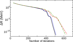
Figure 3: Convergence of the Lanczos and thick-restart Lanczos methods in the case of the 32nd lowest eigenvalue of ⁴⁸Cr with the GXPF1A interaction. The deviation of the 32nd lowest Ritz value from the exact eigenvalue ($\Delta R$) is shown against the number of Lanczos iterations. The solid black line is provided by the Lanczos method, while the convergence of the thick-restart Lanczos method is denoted by the blue dotted ($l_{s}=40,l_{m}=100$), green dot-dashed ($l_{s}=40,l_{m}=50$), and red dashed ($l_{s}=36,l_{m}=50$) lines.

While the thick-restart method can be used to reduce the reorthogonalization cost, the frequent restarts may deteriorate the convergence. We discuss the convergence of the thick-restart Lanczos method in Fig. 3. In the figure the deviation between the 32nd lowest Ritz value and the exact eigenvalue is shown. Hereafter, we focus on the convergence only of the 32nd eigenvalue without particular mention. The number of iterations means the number of accumulated Lanczos steps, not the number of restarts. The thick-restart Lanczos method with $l_{s}=40$ and $l_{m}=100$ shows reasonably fast convergence and requires modest storage (100 Lanczos vectors), while small $l_{m}$ ($l_{m}=50$) deteriorates the convergence since the restart occurs too frequently. The small $l_{s}$ ($l_{s}=36$) also deteriorates the convergence due to the loss of the components at the restart.

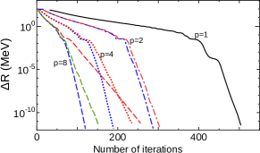
Figure 4: Convergence of the block Lanczos and thick-restart block Lanczos methods. The deviation of the 32nd lowest Ritz value from the exact eigenvalue ($\Delta R$) is shown against the number of iterations. The solid line denotes the convergence of the simple Lanczos method. The convergences of the block Lanczos method are denoted by the blue dot-dashed ($p=2$), dotted ($p=4$), and dashed ($p=8$) lines, respectively, with $p$ being the block size. The corresponding results of the thick-restart block Lanczos method to restrict the storage size up to the 100 Lanczos vectors ($l_{m}=100$) are shown by the red lines. The green dashed line denotes the $p=8$ convergence with $l_{m}=200$ and $l_{s}=40$. See the caption of Fig. 3 for further details.

Figure 4 shows the convergence of the Ritz values by the block Lanczos and thick-restart block Lanczos methods. In the block method, the number of iterations is equal to the number of products of the matrix and block vectors. While the $p=1$ line shows the results of the simple Lanczos method, those of the block Lanczos method with the block sizes $p=2,4,$ and 8 are shown as the blue lines and reach convergence in a small number of iterations. For the block method, the number of iterations for convergence is almost equal and slightly larger than $1/p$ of the simple Lanczos method. It means that the total number of the Lanczos vectors needed in the block method is slightly larger than that of the simple Lanczos method. This additional cost is overwhelmed by the acceleration of the product of the matrix and a block of vectors, the details of which are discussed in the next subsection.

The restart algorithm enables us to decrease the number of Lanczos vectors to be stored, and the cost of the reorthogonalization. The red line in Fig. 4 shows the convergence of the thick-restart block Lanczos method with the number of vectors restricted up to 100 ($l_{m}=100$). While the convergence becomes slightly slow in comparison with the block Lanczos method in the case of $p=2$ and $p=4$, this additional cost is compensated by the speedup of the reorthogonalization. However, in the case of $p=8$ with $l_{m}=100$, the convergence is quite slow since the restart occurs too frequently. The $p=8$ case with the $l_{m}=200$ reduces the number of the iterations and it approaches that of the block Lanczos method without restart.

IV.2 Performance of the block algorithm

In the previous section, we showed that the block algorithm decreases the number of iterations drastically. However, since the elapsed time of a product of a matrix and a block of the vectors increases with $p$, the total performance depends on the balance of the number of iterations and the increased cost of the matrix-block product. In this subsection, we describe some examples of this trade-off. Besides, the thick-restart algorithm also causes a trade-off between the reorthogonalization cost and the number of iterations. The detail of the latter trade-off is discussed in Appx. C.2.

In the KSHELL code, in order to save the memory size the matrix-vector product is realized by the on-the-fly generation of the matrix elements discussed in Appx. B. In order to reduce the additional cost of this generation we adopt the block algorithm. In the usual Lanczos method, the matrix elements are generated on the fly at every matrix-vector product. On the other hand, in the block algorithm, the generation is done once for a bundle of vectors, which are taken as a block. Thus, the block algorithm is expected to reduce the total elapsed time.

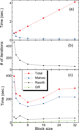
Figure 5: Performance of the thick-restart block Lanczos method to obtain the 32 lowest eigenvalues of ⁴⁸Cr with the GXPF1A interaction with the KSHELL code. (a) Elapsed time of a product of the matrix and the block vectors. The red circles denote the time of a product of a matrix and a block vectors against the block size $p$. The blue triangles denote the elapsed time per vector. The dotted lines are drawn to guide the eyes. (b) The number of iterations for convergence. (c) The red circles, blue squares, black triangles, and green inverted triangles denote the times for total computation, products of the matrix and block vectors, reorthogonalization, and QR-decomposition, respectively.

Figure 5 (a) shows the elapsed time of a product of the matrix and a block of vectors in the LSSM of ⁴⁸Cr, which was also discussed in the previous subsection. The performance was measured by the KSHELL code on 20 CPU cores of Intel Xeon E5-2680. All the Lanczos vectors are stored on memory. In the case of $p=1$ corresponding to the simple Lanczos method, one matrix-vector product costs 0.73 sec. By increasing $p$, the time increases and can be fitted by a line. The $y$-intercept of the fitted line, 0.6 seconds, is the overhead cost of the on-the-fly generation of the matrix elements. This overhead cost is fixed and rather independent of $p$. Therefore, as $p$ increases this overhead cost becomes negligible relative to the time of a matrix product per vector (blue triangle in Fig.5 (a)). As $p$ increases, the time per vector approaches 0.13 seconds, which corresponds to the gradient of the red fitted line.

Figure 5 (b) shows the number of iterations of the thick-restart block Lanczos method to obtain the lowest 32 eigenvalues of ⁴⁸Cr. It decreases drastically as a function of the block size $p$, and reaches 53 at $p=32$, which is almost 1/9 smaller than the case of $p=1$, 466.

Figure 5 (c) shows the total elapsed time of the LSSM of the ⁴⁸Cr case as a function of $p$. The $p=8$ case shows the shortest time, which is determined by the trade-off between the number of iterations and the time of a product of the matrix and a block of vectors. The total time of the products of the matrix and block vectors is shown in the figure and occupies roughly 80% of the total elapsed time.

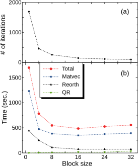
Figure 6: Performance to obtain the 128 lowest eigenvalues of ⁴⁸Cr using the thick-restart block Lanczos method with $l_{m}=800$. See caption of Figs. 5 (b) and (c) for details.

The acceleration caused by the thick-restart block Lanczos method is more effective when a larger number of the eigenvalues are computed. Figure 6 shows the elapsed time to obtain the 128 lowest eigenvalues utilizing the thick-restart block Lanczos method with $l_{m}=800$. The other conditions are the same as Fig. 5. The $p=16$ case reaches the shortest time and provides us with 3.5 times speedup in comparison with the thick-restart Lanczos method. Without the thick restart, the number of the Lanczos vectors increases to 2240 for $p=8$ and the cost of the reorthogonalization extends the total elapsed time by 20% when the whole Lanczos vectors are stored on memory.

We also performed a benchmark test of the system without valence protons, which means that the proton-neutron factorization in Sect. B.2 does not work. In such case the cost of the on-the-fly matrix-elements generation is dominant over the total elapsed time and the block algorithm is advantageous. As such an example we take ¹¹²Sn with the $50\leq N\leq 82$ model space, namely 12 active neutrons in the $0g_{7/2},1d_{5/2},1d_{3/2},2s_{1/2},$ and $0h_{11/2}$ single-particle orbits. Its $M$-scheme dimension is 6,210,638. The SNBG3 interaction is adopted snbg3 ; La133-palit .

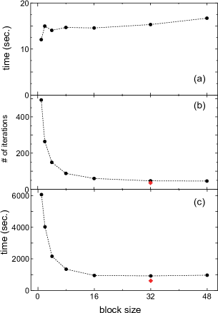
Figure 7: Performance of the thick-restart block Lanczos method to obtain the 32 lowest states of ¹¹²Sn with the SNBG3 interaction snbg3 . The computation was performed at a single node of Oakforest-PACS computer. (a) Elapsed time of the products of the matrix and the block vectors of ¹¹²Sn as a function of the block size. The number of the Lanczos iterations (b) and the elapsed time (c) are shown as the black circles. The red diamond shows the best performance by utilizing the initial vectors which are prepared by the particle-hole truncated approximation. See text for details.

Figure 7 (a) shows the elapsed times of a product of the Hamiltonian matrix and a block of vectors. It was performed on a single node of the Oakforest-PACS computer equipped with 68 CPU cores of Intel Xeon Phi 7250 oakforest-pacs . The code runs with 272 threads for hyperthreading. Unlike the case of ⁴⁸Cr, the elapsed time shows small dependence on the size of the block since it is dominated by the cost of the on-the-fly generation. Therefore the acceleration of the block algorithm is expected to increase in this case. Ideally the relation between the time and the block size should be linear, but fluctuations are seen possibly because of the cache-related matter.

Figure 7 (b) shows the number of iterations to reach the convergence of the 32 lowest eigenvalues as a function of the block size $p$. The number of the iterations drastically decreases as $p$ increases, and it reaches the smallest one, 47, at $p=32$. As the number of iterations decreases the elapsed time also decreases drastically as shown in Fig. 7 (c).

In these benchmarks so far the elements of the initial vectors are taken randomly. On the other hand, well-approximated wave functions can also be used as initial vectors and are expected to accelerate the convergence in the block method. As a benchmark test, we prepare 32 initial vectors by diagonalizing the Hamiltonian in the truncated subspace up to 4-particle 4-hole excitation across the $N=64$ subshell gap. The computation time with the truncated subspace is negligibly small. The red diamonds in Fig. 7 show the best case utilizing those well-approximated initial vectors. As a consequence, this best case takes 672 seconds which is much accelerated in comparison with the case without block algorithm, 6,077 seconds. Note that such a remedy cannot be applied to the simple Lanczos method since the Lanczos method can use only one initial guess.

V Summary

We introduced the thick-restart block Lanczos method as an eigensolver for large-scale shell-model calculations and discussed its performance in comparison with the conventional Lanczos method. Especially when a large number of eigenvalues are required, the block method drastically reduces the number of iterations and the additional cost of the on-the-fly generation of the matrix elements in the KSHELL code. Moreover, the thick-restart algorithm restricts the number of Lanczos vectors and reduces the cost of the reorthogonalization.

The $M$-scheme shell-model code KSHELL was developed for massively parallel computation and is advantageous to obtain highly excited states thanks to the thick-restart block Lanczos method. We demonstrated that the thick-restart block Lanczos method succeeds in reducing the elapsed time of the LSSM calculations by utilizing the KSHELL code taking ⁴⁸Cr and ¹¹²Sn as examples. The performance of the KSHELL code is further discussed in the appendices.

It would be interesting to discuss the nuclear finite-temperature properties using the Lanczos methods ft-lanczos . Pursuing the possibility of the block algorithm, the block Sakurai-Sugiura method using the z-Pares package block-ss ; z-pares provides us with promising results, which will be reported in another publication.

Appendix A $M$-scheme basis states and partitions

The code development plays a key role to develop a frontier of the LSSM calculations. In the last two decades, more than a dozen of shell-model codes had been developed (e.g. ANTOINE antoine , BIGSTICK bigstick , EICODE eicode , KSHELL kshell , NATHAN nathan , NuSHELL nushell ; nushellx , MFDn MFDn ; mfdn-lobpcg , MSHELL64 mshell ; mshell64 , OXBASH oxbash , and VECSSE vecsse ), while their algorithms are different with each other in details.

In the present appendix, we describe the $M$-scheme basis states and how to treat them in the KSHELL code, which was written from scratch in Fortran 95 and Python version 2.6 and is applicable for massively parallel computation. For parallel computation, the $M$-scheme basis states are divided into small groups classified by the number of occupations and the $z$-component of the proton angular momentum. This group is called “partition” and will be discussed later.

The $M$-scheme basis state is defined in Eq. (1). A set of the occupied state $(a_{i,1},a_{i,2},a_{i,3},\cdots,a_{i,A})$ is expressed numerically with occupied and unoccupied states being the bit 1 and bit 0 on the KSHELL code.

$j$	$d_{5/2}$						$s_{1/2}$
# \$m$	-5/2	-3/2	-1/2	1/2	3/2	5/2	-1/2	1/2	$\textbf{N}^{(p)}$
1	1	0	0	1	0	1	0	0	(3,0)
2	0	1	1	0	0	1	0	0
3	0	1	0	1	1	0	0	0
4	1	0	0	0	0	1	0	1	(2,1)
5	0	1	0	0	1	0	0	1
6	0	1	0	0	0	1	1	0
7	0	0	1	1	0	0	0	1
8	0	0	1	0	1	0	1	0
9	0	0	0	1	0	0	1	1	(1,2)

Table 1: Bit representation of the $M$-scheme basis states. It represents all the basis states of three particles occupying the $d_{5/2}$ and $s_{1/2}$ orbits having total $z$-component of the angular momentum $M=1/2$. “1” and “0” denote occupied and unoccupied states, respectively. The leftmost column denotes a serial number of each basis state. The rightmost column shows the occupation numbers of the $d_{5/2}$ and $s_{1/2}$ orbits.

As an example, we show a bit representation of the system in which three identical particles occupy the $d_{5/2}$ and $s_{1/2}$ single-particle orbits in Table 1. The $d_{5/2}$ ($s_{1/2}$) orbit consists of the $m=-\frac{5}{2},-\frac{3}{2},-\frac{1}{2},\frac{1}{2},\frac{3}{2}$ and $\frac{5}{2}$ ($m=-\frac{1}{2}$ and $\frac{1}{2}$) single-particle states where $m$ denotes the $z$-component of the angular momentum of the single-particle state. The table shows the 9 Slater determinants having total $M=\frac{1}{2}$. Each $M$-scheme Slater determinant is expressed as a binary number of which 0 and 1 denote the unoccupied and occupied states, respectively. These 9 determinants are divided into three groups, $\textbf{N}^{(p)}$=(3,0), (2,1), and (1,2), which are the occupation numbers of the $d_{5/2}$ and the $s_{1/2}$ orbits. Each Slater determinant is labeled by a serial number, which is shown in the leftmost column of Table 1. In the practical algorithm, we generate and store all binary numbers representing the proton Slater determinants and the neutron Slater determinants. Any Slater determinant is represented as a product of the proton and the neutron Slater determinants.

In order to apply an arbitrary truncation scheme and to perform parallel computations efficiently, we split whole the $M$-scheme space into small partitions by specifying the occupation numbers of each single-particle orbit and the $z$-component of angular momentum of protons $M^{\pi}$. The practical computation is performed in units of the partitions. The occupation numbers of proton single-particle orbits and neutron single-particle orbits are written as $\textbf{N}^{(p)}=(N^{(p)}_{1},N^{(p)}_{2},...)$ and $\textbf{N}^{(n)}=(N^{(n)}_{1},N^{(n)}_{2},...)$, where the subscript denotes the index of the single-particle orbits in the model space. A partition is specified by $\Gamma=(\textbf{N}^{(p)},\textbf{N}^{(n)},M^{(p)})$. Note that the parity quantum number is specified by $\textbf{N}^{(p)}$ and $\textbf{N}^{(n)}$ uniquely.

The $M$-scheme subspace in a partition is written as a product of the proton $M$-scheme space $(\textbf{N}^{(p)},M^{(p)})$ and the neutron $M$-scheme space, $(\textbf{N}^{(n)},M^{(n)}=M^{\textrm{tot}}-M^{(p)})$, as

$$|M_{i}\rangle=|M^{(p)}_{p_{i}}\rangle\otimes|M^{(n)}_{n_{i}}\rangle,$$ (21)

where $p_{i}$ and $n_{i}$ are the indices of a proton partition $(\textbf{N}^{(p)},M^{(p)})$ and a neutron partition $(\textbf{N}^{(n)},M^{\textrm{tot}}-M^{(p)})$, respectively. The $M$-scheme basis index $i$ is labeled by $(\textbf{N}^{(p)},\textbf{N}^{(n)},M^{(p)},p_{i},n_{i})$. Figure 8 shows a schematic view of the $M$-scheme vector concerning partitions. A vector in the $M=0$ subspace is split into the partitions indicated by the shaded boxes in the figures. Each block is specified by $(\textbf{N}^{(p)},\textbf{N}^{(n)},M^{(p)})$.

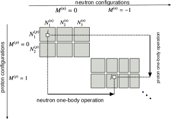
Figure 8: Conceptual drawing of the partitions and the proton-neutron factorization of a vector $v_{i}$ with $M^{(p)}+M^{(n)}=0$. Each shaded box denotes a partition specified by $(\textbf{N}^{(p)},\textbf{N}^{(n)},M^{(p)})$. See text for further details.

In the case of nuclear shell-model calculations, the Hamiltonian matrix $H_{ij}$ is very sparse since the Hamiltonian consists only of one-body and two-body interactions and the matrix element between two Slater determinants in which more than two particles occupy different states is always zero. Especially in medium-heavy nuclei, the $M$-scheme dimension of the Hamiltonian matrix is often quite huge but sparse. Since the matrix is quite sparse and only a few low-lying eigenstates are needed in many LSSM calculations, the Lanczos method has been widely used.

In the $M$-scheme code, we solve the eigenvalue problem in the subspace having good quantum numbers, the $z$-component of total angular momentum $M$ and the parity $\pi$. In addition, the shell-model Hamiltonian has the other symmetry, namely, total angular momentum squared, $J^{2}$. The resultant eigenvector becomes the eigenvector of $J^{2}$ after convergence. When only states having a specified eigenvalue of $J^{2}$ are required, at every Lanczos iteration we can project out the Lanczos vector to the good $J^{2}$ subspace by the Lanczos diagonalization of $J^{2}$ caurier_rmp ; mizusaki-ss .

Appendix B On-the-fly algorithm of the matrix-vector product

The matrix-vector multiplication is the most time-consuming operation in the LSSM calculations. The Hamiltonian matrix is very sparse but requires a huge size of memory if the whole matrix is stored. In order to store the whole Hamiltonian matrix, e.g., in the case of ⁵⁶Ni in the $pf$ shell, whose $M$-scheme dimension is 1,087,455,228, it is required to store $1.2\times 10^{12}$ non-zero matrix elements bigstick , namely, 14.4 TB storage in the compressed sparse raw format and it is impractical. In the KSHELL code, in order to avoid storing the Hamiltonian matrix explicitly we adopt the “on-the-fly” algorithm whose basic idea was suggested in the 1970s and has been used till now M-lanczos ; vecsse ; caurier_rmp . Such on-the-fly method is utilized in several codes, such as ANTOINE code antoine and MSHELL64 mshell64 . In this section, we briefly describe how to implement the matrix-vector product without storing the Hamiltonian matrix elements. In Sect. B.1, the algorithm of the one-body and two-body interactions between identical particles are described. The technique to accelerate the matrix-vector product concerning the proton-neutron interactions utilizing the factorization of the proton and neutron subspaces is discussed in Sect. B.2. This idea of the factorization was further developed in the BIGSTICK code bigstick .

B.1 Interaction between identical particles

In this appendix, we describe how the matrix-vector product is implemented in the case of proton-proton or neutron-neutron interactions. Each $M$-scheme Slater determinant $|M_{i}\rangle$ in Eq.(1) is identified as a binary number: an occupied single-particle state of $|M_{i}\rangle$ is presented as “bit 1”, and an unoccupied state is “bit 0”.

The operation of the two-body interaction is performed by bitwise operations. For example, the operation of a two-body term on the $i$-th vector element is

$$v^{\prime}_{j}|M_{j}\rangle=h^{(2)}_{abcd}c^{\dagger}_{a}c^{\dagger}_{b}c_{d}c_{c}v_{i}|M_{i}\rangle,$$ (22)

where the binary number of $M_{j}$ is obtained as the bit creation of $a$-th and $b$-th bits and the bit annihilation of $c$-th and $d$-th bits. When $a,b,c,d$ and $M_{i}$ are given, we obtain the binary number of $M_{j}$ and subsequently its serial number, $j$, is determined by the binary search to find the $M_{j}$ in the table such as Tab. 1, which is one of the most time-consuming parts. The $v^{\prime}_{j}$ is obtained as $v^{\prime}_{j}=sh^{(2)}_{abcd}v_{i}$ with $s$ being a sign due to the anti-commutation relation. The case of one-body interaction is obtained in the same way straightforwardly.

B.2 Factorization of the proton and neutron spaces

The $M$-scheme model space is spanned by the summation of the partitions, each of which is constructed as a factorization of the proton and neutron subspaces such as Eq. (21). The conceptual drawing of the vector $v_{i}$ is shown in Fig. 8.

The operation of the two-body proton-neutron interaction on the $i$-th vector element is

$$v^{\prime}_{j}|M_{j}\rangle = h_{abcd}c^{\dagger}_{a}c^{\dagger}_{b}c_{d}c_{c}v_{i}|M_{i}\rangle,$$ (23)

$$= h_{abcd}v_{i}c^{\dagger}_{a}c_{c}|M^{(p)}_{p_{i}}\rangle\ c^{\dagger}_{b}c_{d}|M^{(n)}_{n_{i}}\rangle$$

$$= h_{abcd}v_{i}|M^{(p)}_{p_{j}}\rangle\ |M^{(n)}_{n_{j}}\rangle$$

where $a$ and $c$ ($b$ and $d$) denote single-particle states of protons (neutrons). Thus, the operation of the proton-neutron interaction causes the product of proton one-body and neutron one-body operations.

In practical computation, we calculate and store all proton (neutron) one-body operation $|M^{(p)}_{p_{j}}\rangle=c^{\dagger}_{a}c_{c}|M^{(p)}_{p_{i}}\rangle$ ($|M^{(n)}_{n_{j}}\rangle=c^{\dagger}_{b}c_{d}|M^{(n)}_{n_{i}}\rangle$) for every partition. These proton and neutron one-body operations are called “one-body jumps” in Ref. bigstick . By using these one-body jumps, we perform the summation in Eq. (22) so that we avoid computing the two-body jump in each basis.

Figure 8 shows the conceptual drawing of the factorization algorithm. The proton and neutron one-body operations are denoted as the solid arrows.

Appendix C Parallel computation and its performance

The KSHELL code enables us to perform massively parallel computation with hybrid MPI/OpenMP kshell . Figures 9 (a) and (b) show the strong scaling of the parallel computation: the inverse of the elapsed time to the number of nodes for parallel computations. It shows the elapsed time to obtain the ground-state energy of ⁵⁶Ni in $pf$ shell, the $M$-scheme dimension of which reaches around $1.1\times 10^{9}$. These figures show good parallel performance up to $O(10^{4})$ threads and it takes only 192 seconds for the convergence utilizing Oakforest-PACS 96 nodes oakforest-pacs .

Figure 9: Parallel performance at (a) Oakforest-PACS oakforest-pacs and (b) K computer kcomputer . The elapsed time to obtain the ground-state energy of ⁵⁶Ni with the GXPF1A interaction gxpf1a . The dotted lines are drawn to guide the eyes.

The most time-consuming parts of the LSSM calculations are the matrix-vector product and the reorthogonalization (see Figs. 5 and 6). Especially in parallel computation, the elapsed time of the matrix-vector products exceeds 80% of the total elapsed time in most cases, and it is worth discussing how to compute the matrix-vector product in parallel and its parallel efficiency. The parallel computations of the matrix-vector product are discussed in Appx. C.1 and the parallel performance of the reorthogonalization is discussed in Appx. C.2.

C.1 Parallel computation of a matrix-vector product

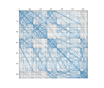
Figure 10: Structure of the Hamiltonian matrix for the $M^{\pi}=0^{+}$ space of ²⁰Ne with the $sd$-shell model space. The only non-zero matrix elements are shown as the blue points. The black lines denote the borders of the partitions of $(\textbf{N}^{(p)},\textbf{N}^{(n)},M^{(p)})$.

Figure 10 shows the non-zero matrix elements of the Hamiltonian matrix of ²⁰Ne with the $sd$-shell model space. While the $M$-scheme dimension is 640, the number of the non-zero matrix elements is 54,104 and thus its sparsity is 13.2%. The black lines denote the borders of the partition $(\textbf{N}^{\pi},\textbf{N}^{\nu},M^{\pi})$. The number of the partitions is 162$\times$162, which are used as units for the parallel computation, and we exclude the computation between the partitions that contain no matrix elements in advance. The order of the partitions are shuffled to achieve good load balance for practical parallel computations.

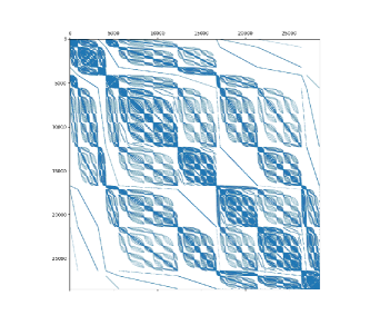
Figure 11: Structure of the Hamiltonian matrix for the $M^{\pi}=0^{+}$ space of ²⁴Mg with the $sd$-shell model space. The only non-zero matrix elements are shown as the blue points.

Figure 11 shows the non-zero matrix elements of the Hamiltonian matrix of ²⁴Mg with the $sd$-shell model space. While the $M$-scheme dimension is 28,503, the number of the non-zero matrix elements is 6,030,189 and thus its sparsity is 0.7%. The sparsity tends to decrease as the $M$-scheme dimension increases. The figure represents that the block structure appears based on the partitions and block diagonal part is quite dense in comparison with the non-diagonal part. This tendency favors more in larger-scale calculations. Thus, since the product operation of diagonal partitions costs far more than that of non-diagonal partitions, it is essential to make the operation of diagonal partitions equally distributed. The number of the partitions is 1020, which is not shown in the figure for simplicity.

The desired features of the algorithm for the parallel computation of the matrix-vector product are

1. Parallel computation based in units of partitions.

2. Good load balance: since diagonal partitions are computationally expensive, they must be distributed equally.

3. The network communications to transfer Lanczos vectors are minimized.

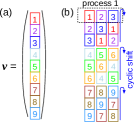
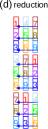
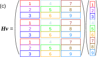
Figure 12: Conceptual drawing of the parallel assignment adopted in the KSHELL code for a matrix-vector product. (a) A Lanczos vector is distributed over nine processes. (b) Data transfer prepared for the matrix-vector product. (c) Assignment on each process for matrix-elements generation in a matrix-vector product. (d) Data transfer after the generation of matrix elements. See text for details.

In order to satisfy these three features, we propose a blocked parallel assignment shown in Fig. 12. In the figure, we assume nine processes for parallel computation and the assignment of each process is shown as colored boxes with the process number.

Here, we describe procedures to perform matrix-vector product in parallel computation. Firstly, a Lanczos vector is split into nine processes equally as shown in Fig. 12(a). In the same manner, each previous Lanczos vector is split into the processes equally and is stored on memory. Secondly, in advance of the matrix-vector product, the required parts of the vector are transferred via MPI communications. In order to perform the product, each process needs other parts of the Lanczos vector in addition to its own part of the vector. For example, the first process requires the first, second, and third parts of the vector, which are transferred by a cyclic shift as shown in Fig. 12(b). Thirdly, the matrix-vector product is performed as shown in Fig. 12(c). The Hamiltonian matrix is split into nine parts as shown in the middle of Fig. 12 so that dense near-diagonal parts of the matrix are distributed to each node equally. Note that the boxes in the matrix in the figure represent the assignments of the on-the-fly generation, not the store of the elements on memory. Finally, the reduction of the resultant parts of the vector is performed via MPI communications shown in Fig. 12(d). In total, the size of the network communication at every matrix-vector product is $16D/\sqrt{N_{p}}$ bytes where $N_{p}$ is the number of parallel nodes and it decreases as $N_{p}$ increases. Such two-dimension topology network communication matches a torus interconnection network adopted in K computer.

For comparison, we mention a simple two-dimensional square-lattice distribution of the matrix. It causes inefficient load balance since the computation of a part handling the diagonal matrix elements costs far heavier than others.

C.2 Parallel computation of reorthogonalization

The parallel computation of the reorthogonalization is rather simple: A Lanczos vector is distributed to all nodes almost equally and the inner product of Lanczos vectors is computed in parallel. Even though the thick-restart algorithm restricts the number of the Lanczos vectors to be orthogonalized, the reorthogonalization is the second time-consuming part of the computation.

If the memory capacity is not enough to store the whole Lanczos vectors (it often occurs in a single-node computation), these vectors are obliged to be stored in the hard disk drive (HDD) and to be read at every reorthogonalization, as done in conventional shell-model codes such as MSHELL64. As the number of iterations increases, the cost of the disk I/O of the HDD grows and it overcomes that of the matrix-vector product as shown in Fig. 13. The block algorithm tends to make the number of the Lanczos vectors larger and gets worse.

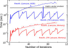
Figure 13: Elapsed time of reorthogonalization against the number of the Lanczos iterations in comparison with the time of a matrix-vector product (black solid horizontal line). The red (blue) dotted line shows the elapsed time of the reorthogonalization of the Lanczos method with storing the Lanczos vectors on memory (on HDD). The solid line shows those with the thick-restart Lanczos method.

Figure 13 shows the time of the reorthogonalization as a function of the number of the Lanczos iterations in the simple Lanczos method utilizing the HDD. The elapsed time was measured to obtain the ground-state energy of the ⁵⁶Ni in the $pf$-shell model space at K computer with 480 nodes kcomputer . The time of the reorthogonalization using the HDD surpasses the time of the matrix-vector product, the black solid line in Fig. 13, at the 39th iteration and becomes the bottleneck. By using the thick-restart method in which the restart process is done when the number of the Lanczos vectors reaches 40, the time of the reorthogonalization (the solid blue line) becomes much smaller than that of the matrix-vector product. However, the thick restart makes the convergence slightly slow as discussed in Sect. IV.1. Some irregular spikes in the figure would be caused by other jobs running at the K computer.

When we store whole the Lanczos vectors on memory, the time of the reorthogonalization is much reduced and is shown as the red lines in Fig. 13. In this case, the time of the reorthogonalization is two orders of magnitude smaller than that of a matrix-vector product, but the memory capacity is required to keep the whole vectors.

References

- (1) M. G. Mayer: Phys. Rev. 75, 1969 (1949); O. Haxel, J. H. D.Jensen, and H. E. Suess: Phys. Rev. 75, 1766 (1949).
- (2) B. A. Brown and B. H. Wildenthal, Annu. Rev. Nucl. Part. Sci. 38, 29 (1988).
- (3) B. A. Brown and W. A. Richter, Phys. Rev. C 74, 034315 (2006).
- (4) M. Honma, T. Otsuka, B. A. Brown, and T. Mizusaki, Eur. Phys. J. A 25, 499 (2005).
- (5) M. Honma, T. Otsuka, T. Mizusaki, and M. H.-Jensen, Phys. Rev. C 80, 064323 (2009).
- (6) T. Otsuka, A. Gade, O. Sorlin, T. Suzuki, and Y. Utsuno, arXiv:1805.06501 [nucl-th]
- (7) E. Caurier, G. Martínez-Pinedo, F. Nowacki, A. Poves, and A. P. Zuker, Rev. Mod. Phys. 77, 427 (2005).
- (8) C. Lanczos, J. Res. Nat. Bur. Stand, 45, 255 (1950).
- (9) K. Wu and H. Simon, SIAM. J. Matrix Anal. & Appl., 22(2), 602 (2000).
- (10) T. Mizusaki, K. Kaneko, M. Honma, and T. Sakurai, Phys. Rev. C 82, 024310 (2010).
- (11) T. Sakurai and H. Sugiura, J. Comp. Appl. Math. 159, 119 (2003).
- (12) M. Shao, H. M. Aktulga, C. Yang, E. G. Ng, P. Maris, and J. P. Vary, Comp. Phys. Comm. 222, 1 (2018).
- (13) E. Caurier and F. Nowacki, Acta Phys. Pol. B 30, 705 (1999)
- (14) J. Toivanen, Computer code EICODE, JYFL, Finland, 2004. arXiv: nucl-th/0610028.
- (15) N. Shimizu, arXiv:1310.5431 [nucl-th]. https://sites.google.com/a/cns.s.u-tokyo.ac.jp/kshell/
- (16) F. Nowacki and E. Caurier, coupled code NATHAN, Strasbourg, 1995.
- (17) C. W. Johnson, W. E. Ormand, and P. G. Krastev, Comp. Phys. Comm. 184, 2761 (2013).
- (18) B. A. Brown and W. D. M. Rae, NUSHELL@MSU, MSU NSCL Report, 2007 (unpublished).
- (19) W. Rae, NuShellX, http://www.garsington.eclipse.co.uk/
- (20) P. Maris, M. Sosonkina, J. P. Vary, E. Ng, and C. Yang, Procedia Comp. Sci. 1, 97 (2010); J.P. Vary, P. Maris, E. Ng, C. Yang, and M. Sosonkina, J. Phys.: Conf. Ser. 180, 012083 (2009).
- (21) T. Mizusaki, RIKEN Accel. Prog. Rep. 33, 14 (2000).
- (22) T. Mizusaki, N. Shimizu, Y. Utsuno, and M. Honma, code MSHELL64, unpublished.
- (23) B. A. Brown, A. Etchegoyen, and W. D. M. Rae, computer code OXBASH, the Oxford University-Buenos Aires-MSU shell model code, Michigan State University Cyclotron Laboratory Report No. 524, 1985.
- (24) T. Sebe and T. Otsuka: code VECSSE, Tokyo (1994).
- (25) A. Spyrou et al., Phys. Rev. Lett. 113, 232502 (2014).
- (26) K. Sieja, Phys. Rev. Lett. 119, 052502 (2017).
- (27) J. E. Midtbø, A. C. Larsen, T. Renstrøm, F. L. Bello Garrote, and E. Lima, Phys. Rev. C 98, 064321 (2018).
- (28) N. Shimizu, Y. Utsuno, Y. Futamura, T. Sakurai, T. Mizusaki and T. Otsuka, Phys. Lett. B 753, 13 (2016).
- (29) Md. S. R. Laskar, S. Saha, R. Palit, S. N. Mishra, N. Shimizu, Y. Utsuno, E. Ideguchi, Z. Naik, F. S. Babra, S. Biswas, S. Kumar, S. K. Mohanta, C. S. Palshetkar, P. Singh, and P. C. Srivastava, Phys. Rev. C 99, 014308 (2019).
- (30) N. Tsunoda, T. Otsuka, N. Shimizu, M. H.-Jensen, K. Takayanagi, and T. Suzuki, Phys. Rev. C 95, 021304(R) (2017).
- (31) J. Cullum, Rep. RC 6827, IBM Thomas J. Waston Research Center, Yorktown Heights, NY, (1977).
- (32) G. H. Golub, and R. Underwood, Proceedings of a Symposium Conducted by the Mathematics Research Center, the University of Wisconsin-Madison, Pages 361-377 (1977).
- (33) Z. Jia, Numer. Math. 80, 239 (1998).
- (34) B. A. Brown, Prog. Part. Nucl. Phys. 47, 517 (2001).
- (35) P. Navrátil, J. P. Vary, and B. R. Barrett, Phys. Rev. Lett. 84, 5728 (2000); Phys. Rev. C 62, 054311 (2000); S. Quaglioni and P. Navrátil, Phys. Rev. Lett. 101, 092501 (2008); Phys. Rev. C 79, 044606 (2009).
- (36) P. Maris, A. M. Shirokov, and J. P. Vary, Phys. Rev. C 81, 021301(R) (2010).
- (37) R.R. Whitehead, Nucl. Phys. A182, 290 (1972).
- (38) T. Sebe and J. Nachamkin, Ann. Phys. 51, 100 (1969).
- (39) For review: Z. Bai, Appl. Num. Math. 43, 9 (2002).
- (40) A. El Guennouni, K. Jbilou, and A. J. Riquet, Numer. Algor. 29, 75 (2002).
- (41) W. H. Press, S. A. Teukolsky, W. T. Vetterling, and B. P. Flannery, Numerical Recipes in FORTRAN, Cambridge University Press, Cambridge (1992).
- (42) J. Baglama, D. Calvetti, L. Reichel, and A. Ruttan, J. Comput. Phys. 146, 203 (1998).
- (43) Z. Teng and L.-H. Zhang, Elec. Trans. Num. Anal. 46, 505 (2017).
- (44) W. Jiang and G. Wu, Comp. Math. Appl., 60, 873 (2010).
- (45) J. Baglama and L. Reichel, Numer. Algor. 43, 251 (2006).
- (46) M. Honma et al., RIKEN Accel. Prog. Rep. 45, 35 (2012); M. Honma (private communication).
- (47) Oakforest-PACS supercomputer system, https://www.cc.u-tokyo.ac.jp/en/supercomputer/ofp/service/
- (48) J. Jaklič and P. Prelovšek, Phys. Rev. B 49, 5065(R) (1994).
- (49) T. Ikegami, T. Sakurai, and U. Nagashima, J. Comput. Appl. Math. 233, 1927 (2010).
- (50) Y. Futamura, and T. Sakurai, “z-Pares: Parallel Eigenvalue Solver”, http://zpares.cs.tsukuba.ac.jp/.
- (51) K computer, RIKEN Center for Computational Science, https://www.r-ccs.riken.jp/en/k-computer/about/