On ADMM in Deep Learning: Convergence and Saturation-Avoidance

Abstract

In this paper, we develop an alternating direction method of multipliers (ADMM) for deep neural networks training with sigmoid-type activation functions (called sigmoid-ADMM pair), mainly motivated by the gradient-free nature of ADMM in avoiding the saturation of sigmoid-type activations and the advantages of deep neural networks with sigmoid-type activations (called deep sigmoid nets) over their rectified linear unit (ReLU) counterparts (called deep ReLU nets) in terms of approximation. In particular, we prove that the approximation capability of deep sigmoid nets is not worse than that of deep ReLU nets by showing that ReLU activation function can be well approximated by deep sigmoid nets with two hidden layers and finitely many free parameters but not vice-verse. We also establish the global convergence of the proposed ADMM for the nonlinearly constrained formulation of the deep sigmoid nets training from arbitrary initial points to a Karush-Kuhn-Tucker (KKT) point at a rate of order ${\cal O}(1/k)$. Besides sigmoid activation, such a convergence theorem holds for a general class of smooth activations. Compared with the widely used stochastic gradient descent (SGD) algorithm for the deep ReLU nets training (called ReLU-SGD pair), the proposed sigmoid-ADMM pair is practically stable with respect to the algorithmic hyperparameters including the learning rate, initial schemes and the pro-processing of the input data. Moreover, we find that to approximate and learn simple but important functions the proposed sigmoid-ADMM pair numerically outperforms the ReLU-SGD pair.

Keywords: Deep learning, ADMM, sigmoid, global convergence, saturation avoidance

1 Introduction

In the era of big data, data of massive size are collected in a wide range of applications including image processing, recommender systems, search engineering, social activity mining and natural language processing (Zhou et al., 2014). These massive data provide a springboard to design machine learning systems matching or outperforming human capability but pose several challenges on how to develop learning systems to sufficiently exploit the data. As shown in Figure 1, the traditional approach comes down to a three-step learning process. It at first adopts delicate data transformations to yield a tractable representation of the original massive data; then develops some interpretable and computable optimization models based on the transformed data to embody the utility of data; finally designs efficient algorithms to solve the proposed optimization problems. These three steps are called feature extraction, model selection and algorithm designation respectively. Since feature extraction usually involves human ingenuity and prior knowledge, it is labor intensive, especially when the data size is huge. Therefore, it is highly desired to reduce the human factors in the learning process.

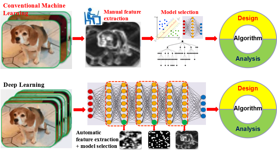
Figure 1: Philosophy behind deep learning

Deep learning (Hinton and Salakhutdinov, 2006; LeCun et al., 2015), which utilizes deep neural networks (deep nets for short) for feature extraction and model selection simultaneously, provides a promising way to reduce human factors in machine learning. Just as Figure 1 purports to show, deep learning transforms the classical three-step strategy into a two-step approach: neural networks selection and algorithm designation. It is thus important to pursue why such a transformation is feasible and efficient. In particular, we are interested in making clear of when deep nets are better than classical methods such as shallow neural networks (shallow nets) and kernel methods, and which optimization algorithm is good enough to realize the benefits brought from deep nets.

In the past decade, deep nets with ReLU activations (deep ReLU nets) equipped with the well known stochastic gradient descent (SGD) algorithm have been successfully used in image classification (Krizhevsky et al., 2012), speech recognition (Hinton et al., 2012; Sainath et al., 2013), natural language processing (Devlin et al., 2014), demonstrating the power of ReLU-SGD pair in deep learning. The problem is, however, that there is a crucial inconsistency between approximation and optimization for the ReLU-SGD pair. To be detailed, from the approximation theory viewpoint, it is necessary to deepen the network to approximate smooth function (Yarotsky, 2017), extract manifold structures (Shaham et al., 2018), realize rotation-invariance features (Han et al., 2020) and provide localized approximation (Safran and Shamir, 2017). However, from the optimization viewpoint, it is difficult to solve optimization problems associated with too deep networks with theoretical guarantees (Goodfellow et al., 2016). Besides the lack of convergence (to a global minima) guarantees, deep ReLU nets equipped with SGD may suffer from the issue of gradient explosion/vanishing (Goodfellow et al., 2016) and is usually sensitive to its algorithmic hyper-parameters such as the initialization (Glorot and Bengio, 2010; Sutskever et al., 2013; Hanin and Rolnick, 2018) and learning rate (Senior et al., 2013; Daniel et al., 2016; Ruder, 2016) in the sense that these parameters have dramatic impacts on the performance of SGD and thus should be carefully tuned in practice. In a nutshell, deep ReLU nets should be deep enough to exhibit excellent approximation capability while too deep networks frequently impose additional difficulty in optimization.

There are numerous remedies to tackle the aforementioned inconsistency for the ReLU-SGD pair with intuition that SGD as well as its variants is capable of efficiently solving the optimization problem associated with deep ReLU nets. In particular, some tricks on either the network architectures such as ResNets (He et al., 2016) or the training procedure such as the batch normalization (Ioffe and Szegedy, 2015) and weight normalization (Salimans and Kingma, 2016) have been developed to address the issue of gradient vanishing/explosion; several efficient initialization schemes including the MSRA initialization (He et al., 2015) have been proposed for deep ReLU nets; some guarantees have been established (Allen-Zhu et al., 2019; Du et al., 2019; Zou and Gu, 2019) in the over-parametrized setting to verify the convergence of SGD; and numerous strategies of learning rates (Chollet et al., 2015; Gotmare et al., 2019; Smith and Topin, 2017) have been provided to enhance the feasibility of SGD.

Different from the aforementioned approach focusing on modifying SGD for deep ReLU nets, we pursue an alternative direction to ease the training via reducing the depth. Our studies stem from an interesting observation in neural networks approximation. As far as the approximation capability is concerned, deep nets with sigmoid-type activation functions (deep sigmoid nets) theoretically perform better than deep ReLU nets for some function classes in the sense that to attain the same approximation accuracy, the depth and number of parameters of the former is much smaller than those of the latter. This phenomenon was observed in approximating smooth functions (Mhaskar, 1996; Yarotsky, 2017), reflecting the rotation invariance feature (Chui et al., 2019; Han et al., 2020) and capturing sparse signals (Lin et al., 2017; Schwab and Zech, 2019).

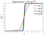
(a) Sigmoid functions

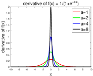
(b) Saturation of sigmoid

(c) SGD vs. ADMM

Figure 2: The cons of SGD and pros of ADMM in solving deep sigmoid nets. The setting of numerical simulation in (c) can be found in the Table 2 below.

In spite of their advantages in approximation, deep sigmoid nets have not been widely used in the deep learning community. The major reason is due to the saturation problem of the sigmoid function (Goodfellow et al., 2016, Section 6.3), which is easy to cause gradient vanishing for gradient-descent based algorithms in the deep sigmoid nets training (Bengio et al., 1994; LeCun et al., 1998). Specifically, as shown in Figure 2 (b), derivatives of sigmoid functions vanish numerically in a large range. In this paper, we aim at developing a gradient-free algorithm for the deep sigmoid nets training to avoid saturation of deep sigmoid nets and sufficiently embody their theoretical advantages. As a typical gradient-free optimization algorithm, alternating direction method of multipliers (ADMM) can be regarded as a primal-dual method based on an augmented Lagrangian by introducing nonlinear constraints and enables a convergent sequence satisfying the nonlinear constraints. Therefore, ADMM attracted rising attention in deep learning with various implementations (Carreira-Perpinan and Wang, 2014; Taylor et al., 2016; Kiaee et al., 2016; Yang et al., 2016; Gotmare et al., 2018; Murdock et al., 2018). Under this circumstance, we propose an efficient ADMM algorithm based on a novel update order and an efficient sub-problem solver. Surprisingly, as shown in Figure 2 (c), the proposed sigmoid-ADMM pair performs better than ReLU-SGD pair in approximating the simple but extremely important square function (Yarotsky, 2017; Petersen and Voigtlaender, 2018; Han et al., 2020). This implies that ADMM may be an efficient algorithm to sufficiently realize theoretical advantages of deep sigmoid nets. Our contributions of this paper can be summarized as the following three folds.

$\bullet$ Methodology Novelty: We develop a novel sigmoid-ADMM pair for deep learning. Compared with the widely used ReLU-SGD pair, the proposed sigmoid-ADMM pair is stable with respect to algorithmic hyperparameters including learning rates, initial schemes and the pro-processing of input data. Furthermore, we find that to approximate and learn simple but important functions including the square function, radial functions and product gate, deep sigmoid nets theoretically beat deep ReLU nets and the proposed sigmoid-ADMM pair outperforms the ReLU-SGD pair. In terms of algorithm designs, different from existing ADMM methods in deep learning, our proposed ADMM adopts a backward-forward update order that is similar as BackProp (Rumelhart et al., 1986) and a local linear approximation for sub-problems, and more importantly keeps all the nonlinear constraints such that the solution found by the proposed algorithm can converge to a solution satisfying these nonlinear constraints.

$\bullet$ Theoretical Novelty: To demonstrate the theoretical advantages of deep sigmoid nets, we rigorously prove that the approximation capability of deep sigmoid nets is not worse than deep ReLU nets by showing that ReLU can be well approximated by deep sigmoid nets with two hidden layers and finitely many free parameters but not vice-verse. We also establish the global convergence of the proposed ADMM for the nonlinearly constrained formulation of the deep sigmoid nets training from arbitrary initial points to a Karush-Kuhn-Tucker (KKT) point at a rate of order ${\cal O}(1/k)$. Different from the existing literature on convergence of nonconvex ADMM (Hong et al., 2016; Wang et al., 2019; Gao et al., 2020) for linear or multiaffine constrained optimization problems, our analysis provides a new methodology to deal with the nonlinear constraints in deep learning. In a word, our approach actually leads to a general convergence framework for ADMM with “smooth” enough activations.

$\bullet$ Numerical Novelty: In terms of numerical performance, the effectiveness (particularly the stability to initial schemes and the easy-to-tune property of algorithmic parameters) of the proposed ADMM has been demonstrated by numerous experiments including a series of toy simulations and three real-data experiments. Numerical results illustrate the outperformance of the sigmoid-ADMM pair over the ReLU-SGD pair in approximating the extremely important square function, product gate, piecewise $L_{1}$ radial and smooth $L_{2}$ radial functions with stable algorithmic hyperparameters. Together with some other important functions such as the localized approximation (Chui et al., 1994), these natural functions realized in this paper can represent some important data features such as piecewise smoothness in image processing (Krizhevsky et al., 2012), sparseness in computer vision (LeCun et al., 2015), and rotation-invariance in earthquake prediction (Vikraman, 2016). The effectiveness of the proposed ADMM is further demonstrated by real-data experiments, i.e., earthquake intensity, extended Yale B databases and PTB Diagnostic ECG databases, which reflect the partially radial and low-dimensional manifold features in some extent.

The rest of this paper is organized as follows. In the next section, we demonstrate the advantage of deep sigmoid nets in approximation (see Theorem 3). Section 3 describes the proposed ADMM method for the considered DNN training model followed by the main convergence theorem (see Theorem 4). Section 4 provides some discussions on related work and key ideas of our proofs. Section 5 provides some toy simulations to show the effectiveness of the proposed ADMM method in realizing some important natural functions. Section 6 provides two real data experiments to further demonstrate the effectiveness of the proposed method. All proofs are presented in Appendix.

Notations: For any matrix $A\in\mathbb{R}^{m\times n}$, $[A]_{ij}$ denotes its $(i,j)$-th entry. Given a matrix $A$, $\|A\|_{F}$, $\|A\|_{2}$ and $\|A\|_{\max}$ denote the Frobenius norm, operator norm, and max-norm of $A$, respectively, where $\|A\|_{\max}=\max_{i,j}|[A]_{ij}|$. Then obviously, $\|A\|_{\max}\leq\|A\|_{2}\leq\|A\|_{F}$. We let $W_{<i}:=[W_{1},W_{2},\ldots,W_{i-1}]$, $W_{>i}:=[W_{i+1},\ldots,W_{N}]$ for $i=1,\ldots,N$, $W_{<1}=\emptyset$ and $W_{>N}=\emptyset$. ${\bf I}$ denotes the identity matrix whose size can be determined according to the text. Denote by $\mathbb{R}$ and $\mathbb{N}$ the real and natural number sets, respectively.

2 Deep Sigmoid Nets in Approximation

For the depth $N\in\mathbb{N}$ of a neural network, let $d_{i}\in\mathbb{N}$ be the number of hidden neurons at the $i$-th hidden layer for $i=1,\ldots,N-1$. Denote an affine mapping ${\cal J}_{i}:\mathbb{R}^{d_{i-1}}\rightarrow\mathbb{R}^{d_{i}}$ by $\mathcal{J}_{i}(x):=W_{i}x+b_{i}$ for $d_{i}\times d_{i-1}$ weight matrix and thresholds $b_{i}\in\mathbb{R}^{d_{i}}$. For a univariate activation function $\sigma_{i},i=1\dots,N$, denote further $\sigma_{i}(x)$ when $\sigma_{i}$ is applied component-wise to the vector $x$. Define an $N$-layer feedforward neural network by

$$\mathcal{N}_{N,d_{1},\dots,d_{N},\sigma}=a\cdot\sigma_{N}\circ\mathcal{J}_{N}\circ\sigma_{N-1}\circ\mathcal{J}_{N-1}\circ\dots\circ\sigma_{1}\circ\mathcal{J}_{1}(x),$$ (1)

where $a\in\mathbb{R}^{d_{N}}$. The deep net defined in (1) is called the deep ReLU net and deep sigmoid net, provided $\sigma_{i}(t)\equiv\sigma_{relu}(t)=\max\{t,0\}$ and $\sigma_{i}(t)\equiv\sigma(t)=\frac{1}{1+e^{-t}}$ respectively.

Since the (sub-)gradient computation of ReLU is very simple, deep ReLU nets have attracted enormous research activities in the deep learning community (Nair and Hinton, 2010). The power of deep ReLU nets, compared with shallow nets with ReLU (shallow ReLU nets) has been sufficiently explored in the literature (Yarotsky, 2017; Petersen and Voigtlaender, 2018; Shaham et al., 2018; Schwab and Zech, 2019; Chui et al., 2020; Han et al., 2020). In particular, it was proved in (Yarotsky, 2017, Proposition 2) that the following “square-gate” property holds for deep ReLU nets, which is beyond the capability of shallow ReLU nets due to the non-smoothness of ReLU.

Lemma 1

The function $f(t)=t^{2}$ on the segment $[-M,M]$ for $M>0$ can be approximated within any accuracy $\varepsilon>0$ by a deep ReLU net with the depth and free parameters of order $\mathcal{O}(\log(1/\varepsilon))$.

The above lemma exhibits the necessity of the depth for deep ReLU nets to act as a “square-gate”. Since the depth depends on the accuracy, it requires many hidden layers for deep ReLU nets for such an easy task and too many hidden layers enhance the difficulty for analyzing SGD (Goodfellow et al., 2016, Sec.8.2). This presents the reason why the numerical accuracy of deep ReLU nets in approximating $t^{2}$ is not so good, just as Figure 2 exhibits. Differently, due to the infinitely differentiable property of the sigmoid function, it is easy for shallow sigmoid nets (Chui et al., 2019, Proposition 1) to play as a “square-gate”, as shown in the following lemma.

Lemma 2

Let $M>0$. For $\varepsilon>0$, there is a shallow sigmoid net $\mathcal{N}_{3}$ with 3 free parameters bounded by $\mathcal{O}(\varepsilon^{-6})$ such that

$$|t^{2}-\mathcal{N}_{3}(t)|\leq\varepsilon,\qquad t\in[-M,M].$$

Besides the “square-gate”, deep sigmoid nets are capable of acting as a “product-gate” (Chui et al., 2019), providing localized approximation (Chui et al., 1994), extracting the rotation-invariance property (Chui et al., 2019) and reflecting the sparseness in spatial domain (Lin, 2019) and frequency domain (Lin et al., 2017) with much fewer hidden layers than deep ReLU nets. The following Table 1 presents a comparison between deep sigmoid nets and deep ReLU nets in feature selection and approximation.

Table 1: Depth required for deep nets in feature extraction and approximation within accuracy $\varepsilon$

Features	sigmoid	ReLU
Square-gate	$1$ (Chui et al., 2019)	$\log(\varepsilon^{-1})$ (Yarotsky, 2017)
Product-gate	$1$ (Chui et al., 2019)	$\log(\varepsilon^{-1})$ (Yarotsky, 2017)
Localized approximation	$2$ (Chui et al., 1994)	$2$(Chui et al., 2020)
$k$-spatially sparse+smooth	$2$ (Lin, 2019)	$>8$ (Chui et al., 2020)
Smooth+Manifold	$3$ (Chui et al., 2018)	$4$ (Shaham et al., 2018)
Smooth	1 (Mhaskar, 1996)	$\log(\varepsilon^{-1})$ (Yarotsky, 2017)
$k$-sparse (frequency)	$k$ (Lin et al., 2017)	$k\log(\varepsilon^{-1})$ (Schwab and Zech, 2019)
Radial+smooth	4 (Chui et al., 2019)	$>8$ (Han et al., 2020)

Table 1 presents theoretical advantages of deep sigmoid nets over deep ReLU nets. In fact, as the following theorem shows, it is easy to construct a sigmoid net with two hidden layers and small number of free parameters to approximate ReLU, implying that the approximation capability of deep sigmoid nets is at least not worse than that of deep ReLU nets with comparable hidden layers and free parameters.

Theorem 3

Let $1\leq p<\infty$ and $M\geq 1$. Then for any $\varepsilon\in(0,1/2)$ and $M>0$, there is a sigmoid net $h^{*}$ with $2$ hidden layers and at most 27 free parameters bounded by $\mathcal{O}(\varepsilon^{-7})$ such that

$$\|h^{*}-\sigma_{relu}\|_{L^{p}([-M,M])}\leq\varepsilon,$$ (2)

where $L^{p}([-M,M])$ denotes the $L^{p}$ space of functions defined on $[-M,M]$.

The proof of Theorem 3 is postponed in Appendix A. For an arbitrary deep ReLU net

$$\mathcal{N}^{relu}_{L,d_{1},\dots,d_{L}}=a\cdot\sigma_{relu}\circ\mathcal{J}_{L}\circ\sigma_{relu}\circ\mathcal{J}_{L-1}\circ\dots\circ\sigma_{relu}\circ\mathcal{J}_{1}(x)$$

with bounded free parameters, Theorem 3 shows that we can construct a deep sigmoid net

$$\mathcal{N}^{sigmoid}_{L,d_{1},\dots,d_{L}}=a\cdot h^{*}\circ\mathcal{J}_{L}\circ h^{*}\circ\mathcal{J}_{L-1}\circ\dots\circ h^{*}\circ\mathcal{J}_{1}(x)$$

that possesses at least similar approximation capability. However, due to the infinitely differentiable property of the sigmoid function, it is difficult to construct a deep ReLU net with accuracy-independent depth and width to approximate it. Indeed, it can be found in (Petersen and Voigtlaender, 2018, Theorem 4.5) that for any open interval $\Omega$ and deep ReLU net $\mathcal{N}^{relu}_{L,n}$ with $L$ hidden layers and $n$ free parameters, there holds

$$\|\sigma-\mathcal{N}^{relu}_{L,n}\|_{L^{p}(\Omega)}\geq C^{\prime\prime}n^{-2L},$$ (3)

where $\sigma$ is the sigmoid activation and $C^{\prime\prime}$ is a constant independent of $n$ or $L$. Comparing (2) with (3), we find that any functions being well approximated by deep ReLU nets can also be well approximated by deep sigmoid nets, but not vice-verse.

It should be mentioned that though the depth and width in Theorem 3 are independent of $\varepsilon$ and relatively small, the magnitude of free parameters depends heavily on the accuracy and may be large. Since such large free parameters are difficult to realize for an optimization algorithm, a preferable way to shrink them is to deepen the network further. In particular, it can be found in (Chui et al., 2019) that there is a shallow sigmoid net $\mathcal{N}^{sigmoid}_{2}$ with 2 free parameters of order $\mathcal{O}(1/\varepsilon)$ such that

$$|\sigma(\sqrt{w}\mathcal{N}^{sigmoid}_{2}(\sqrt{w}t))-\sigma(wt)|\leq\varepsilon,$$

where $t,w\in\mathbb{R}$. Because we only focus on the power of deep sigmoid nets in approximation, we do not shrink free parameters in Theorem 3.

3 ADMM for Deep Sigmoid Nets

Let ${\cal Z}:=\{(x_{j},y_{j})\}_{j=1}^{n}\subset\mathbb{R}^{d_{0}}\times\mathbb{R}^{d_{N}}$ be $n$ samples. Denote $X:=(x_{1},x_{2},\ldots,x_{n})\in\mathbb{R}^{d_{0}\times n}$ and $Y:=(y_{1},y_{2},\ldots,y_{n})\in\mathbb{R}^{d_{N}\times n}$. It is natural to consider the following regularized DNN training problem

$$\min_{\cal W}\left\{\frac{1}{n}\sum_{i=1}^{n}\|\Phi(x_{i},\mathcal{W})-y_{i}\|_{2}^{2}+\lambda^{\prime}\|W_{i}\|_{F}^{2}\right\},$$ (4)

where $\Phi(x_{i},\mathcal{W})$ denotes a deep sigmoid net with $N$ layers, $\mathcal{W}=\{W_{i}\}_{i=1}^{N}$ and $\lambda^{\prime}>0$ is the regularization parameter. Here, we consider the square loss as analyzed in the literature (Allen-Zhu et al., 2019; Du et al., 2019; Zou and Gu, 2019). We also absorb thresholds into the weight matrices for the sake of simplicity. Based on the advantage of deep sigmoid nets in approximation, (Chui et al., 2019; Lin, 2019) proved that the model defined by (4) with $N=2$ are optimal in embodying data features such as the spatial sparseness, smoothness and rotation-invariance in the sense that it can achieve almost optimal generalization error bounds in the framework of learning theory. The aim of this section is to introduce an efficient algorithm to solve the optimization problem (4).

Due to the saturation problem of the sigmoid function (see Figure 2 (b)), the issue of gradient vanishing or explosion frequently happens for running SGD on deep sigmoid nets (see Figure 4 (a) for example), implying that the classical SGD is not a good candidate to solve (4). We then turn to designing a gradient-free optimization algorithm, like ADMM, to efficiently solve (4). For DNN training, there are generally two important ingredients in designing ADMM: update order and solution to each sub-problem. The novelty of our proposed algorithm is the use of backward-forward update order similar to BackProp in (Rumelhart et al., 1986) and local linear approximation to sub-problems.

3.1 Update order in ADMM for deep learning training

The optimization problem (4) can be equivalently reformulated as the following constrained optimization problem

$$\mathop{\mathrm{minimize}}_{{\cal W},{\cal V}}\ \frac{1}{2}\|V_{N}-Y\|_{F}^{2}+\frac{\lambda}{2}\sum_{i=1}^{N}\|W_{i}\|_{F}^{2}$$ (5)

$$\text{subject to}\quad V_{i}=\sigma(W_{i}V_{i-1}),\ i=1,\ldots,N-1,\quad V_{N}=W_{N}V_{N-1},$$

where ${\cal V}:=\{V_{i}\}_{i=1}^{N}$ represents the set of responses of all layers and $\lambda=\frac{\lambda^{\prime}n}{2}$. We define the augmented Lagrangian of (5) as follows:

$${\cal L}({\cal W},{\cal V},\{\Lambda_{i}\}_{i=1}^{N}) :=\frac{1}{2}\|V_{N}-Y\|_{F}^{2}+\frac{\lambda}{2}\sum_{i=1}^{N}\|W_{i}\|_{F}^{2}$$ (6)

$$+\sum_{i=1}^{N-1}\left(\frac{\beta_{i}}{2}\|\sigma(W_{i}V_{i-1})-V_{i}\|_{F}^{2}+\langle\Lambda_{i},\sigma(W_{i}V_{i-1})-V_{i}\rangle\right)$$

$$+\frac{\beta_{N}}{2}\|W_{N}V_{N-1}-V_{N}\|_{F}^{2}+\langle\Lambda_{N},W_{N}V_{N-1}-V_{N}\rangle,$$

where $\Lambda_{i}\in\mathbb{R}^{d_{i}\times n}$ is the multiplier matrix associated with the $i$-th constraint, and $\beta_{i}$ is the associated penalty parameter for $i=1,\ldots,N$.

ADMM is an augmented-Lagrangian based primal-dual method, which updates the primal variables ($\{W_{i}\}_{i=1}^{N}$ and $\{V_{i}\}_{i=1}^{N}$ in (6)) via a Gauss-Seidel scheme and then multipliers ($\{\Lambda_{i}\}_{i=1}^{N}$ in (6)) via a gradient ascent scheme in a parallel way (Boyd et al., 2011). As suggested in (Wang et al., 2019), the update order of the primal variables is tricky for ADMM in terms of the convergence analysis in the nonconvex setting. In light of (Wang et al., 2019), the key idea to yield a desired update order with convergence guarantee is to arrange the updates of some special primal variables followed by the updates of multipliers such that the updates of multipliers can be explicitly expressed by the updates of these special primal variables, and thus the dual ascent quantities arisen by the updates of multipliers shall be controlled by the descent quantities brought by the updates of these special primal variables. Hence, the arrangement of these special primal variables is crucial.

It can be noted that there are $2N$ blocks of primal variables, i.e., $\{W_{i}\}_{i=1}^{N}$ and $\{V_{i}\}_{i=1}^{N}$ and $N$ blocks of multipliers $\{\Lambda_{i}\}_{i=1}^{N}$ involved in (6). For better elaboration of our idea, we take $N=3$ for an example. Notice that the multipliers $\{\Lambda_{i}\}_{i=1}^{3}$ are only involved in these inner product terms $\langle\Lambda_{1},\sigma(W_{1}X)-V_{1}\rangle$, $\langle\Lambda_{2},\sigma(W_{2}V_{1})-V_{2}\rangle$ and $\langle\Lambda_{3},W_{3}V_{2}-V_{3}\rangle$. By these terms, the gradient of the $i$-th inner product with respect to $V_{i}$ is $-\Lambda_{i}$, while the associated gradient with respect to $W_{i}$ is a more complex term (namely, $(\Lambda_{1}\odot\sigma^{\prime}(W_{1}X))X^{T}$ for $W_{1}$, $(\Lambda_{2}\odot\sigma^{\prime}(W_{2}V_{1}))V_{1}^{T}$ for $W_{2}$, and $\Lambda_{3}V_{2}^{T}$ for $W_{3}$, where $\odot$ represents Hadamard product). If the update of $W_{i}$ is used to express $\Lambda_{i}$, then according to the $W_{i}$ subproblem, an inverse operation of a nonlinear or linear mapping is required, while such an inverse does not necessarily exist. Specifically, following the analysis of Lemma 8 shown later and taking the expression of $W_{3}$ for example, the term $\Lambda_{3}V_{2}^{T}$ will be involved in the expression of $W_{3}$. In this case, if we wish to express $\Lambda_{3}$ by $W_{3}$, then the inverse of $V_{2}$ is generally required, while it does not necessarily exist. Due to this, it should be more convenient to express $\Lambda_{i}$ $(i=1,2,3)$ via exploiting the $V_{i}$ subproblem instead of the $W_{i}$ subproblem. Therefore, we suggest firstly update the blocks of $W_{i}$’s and then $V_{i}$’s such that $\Lambda_{i}$’s can be explicitly expressed via the latest updates of $V_{i}$’s. To be detailed, for each loop, we update $\{W_{i}\}_{i=1}^{N}$ in the backward order, i.e., $W_{N}\rightarrow W_{N-1}\rightarrow\cdots\rightarrow W_{1}$, then update $\{V_{j}\}_{j=1}^{N}$ in the forward order, i.e., $V_{1}\rightarrow V_{2}\rightarrow\cdots\rightarrow V_{N}$, motivated by BackProp in (Rumelhart et al., 1986), and finally update the multipliers $\{\Lambda_{i}\}_{i=1}^{N}$ in a parallel way, as shown by the following Figure 3.

Figure 3: Update order of ADMM

Specifically, given an initialization $\{W_{i}^{0}\}_{i=1}^{N}$, we set

$$V_{j}^{0}=\sigma(W_{j}^{0}V_{j-1}^{0}),\ j=1,\ldots,N-1,\quad V_{N}^{0}=W_{N}^{0}V_{N-1}^{0},\ \text{and}\ \Lambda_{i}^{0}=0,\ i=1,\ldots,N,$$ (7)

where $V_{0}^{0}=X$. Given the ($k$-$1$)-th iterate $\Big{(}\{W_{i}^{k-1}\}_{i=1}^{N},\{V_{i}^{k-1}\}_{i=1}^{N},$ $\{\Lambda_{i}^{k-1}\}_{i=1}^{N}\Big{)}$, we define the $W_{i}$- and $V_{i}$-subproblems at the $k$-th iteration via minimizing the augmented Lagrangian (6) with respect to only one block but fixing the other blocks at the latest updates, according to the update order specified in Figure 3, shown as follows:

$$W_{N}^{k}=\arg\min_{W_{N}}\left\{\frac{\lambda}{2}\|W_{N}\|_{F}^{2}+\frac{\beta_{N}}{2}\|W_{N}V_{N-1}^{k-1}-V_{N}^{k-1}\|_{F}^{2}+\langle\Lambda_{N}^{k-1},W_{N}V_{N-1}^{k-1}-V_{N}^{k-1}\rangle\right\},$$ (8)

and for $i=N-1,\ldots,1,$

$$W_{i}^{k}=\arg\min_{W_{i}}\left\{\frac{\lambda}{2}\|W_{i}\|_{F}^{2}+\frac{\beta_{i}}{2}\|\sigma(W_{i}V_{i-1}^{k-1})-V_{i}^{k-1}\|_{F}^{2}+\langle\Lambda_{i}^{k-1},\sigma(W_{i}V_{i-1}^{k-1})-V_{i}^{k-1}\rangle\right\},$$ (9)

and for $j=1,\ldots,N-2$,

$$V_{j}^{k}=\arg\min_{V_{j}}\left\{\frac{\beta_{j}}{2}\|\sigma(W_{j}^{k}V_{j-1}^{k})-V_{j}\|_{F}^{2}+\langle\Lambda_{j}^{k-1},\sigma(W_{j}^{k}V_{j-1}^{k})-V_{j}\right.\rangle$$ (10)

$$\ \ \ \ \ \ \ \ \ \ \ \ \ \ \ \ \ \ \ \ \left.+\frac{\beta_{j+1}}{2}\|\sigma(W_{j+1}^{k}V_{j})-V_{j+1}^{k-1}\|_{F}^{2}+\langle\Lambda_{j+1}^{k-1},\sigma(W_{j+1}^{k}V_{j})-V_{j+1}^{k-1}\rangle\right\},$$

$$V_{N-1}^{k}=\arg\min_{V_{N-1}}\left\{\frac{\beta_{N-1}}{2}\|\sigma(W_{N-1}^{k}V_{N-2}^{k})-V_{N-1}\|_{F}^{2}+\langle\Lambda_{N-1}^{k-1},\sigma(W_{N-1}^{k}V_{N-2}^{k})-V_{N-1}\right.\rangle$$

$$\ \ \ \ \ \ \ \ \ \ \ \ \ \ \ \ \ \ \ \ \left.+\frac{\beta_{N}}{2}\|W_{N}^{k}V_{N-1}-V_{N}^{k-1}\|_{F}^{2}+\langle\Lambda_{N}^{k-1},W_{N}^{k}V_{N-1}-V_{N}^{k-1}\rangle\right\},$$ (11)

$$V_{N}^{k}=\arg\min_{V_{N}}\left\{\frac{1}{2}\|V_{N}-Y\|_{F}^{2}+\frac{\beta_{N}}{2}\|W_{N}^{k}V_{N-1}^{k}-V_{N}\|_{F}^{2}+\langle\Lambda_{N}^{k-1},W_{N}^{k}V_{N-1}^{k}-V_{N}\rangle\right\}.$$ (12)

Once $\left(\{W_{i}^{k}\}_{i=1}^{N},\{V_{i}^{k}\}_{i=1}^{N}\right)$ have been updated, we then update the multipliers $\{\Lambda_{i}^{k}\}_{i=1}^{N}$ parallelly according to the following: for $i=1,\ldots,N-1$,

$$\Lambda_{i}^{k}=\Lambda_{i}^{k-1}+\beta_{i}(\sigma(W_{i}^{k}V_{i-1}^{k})-V_{i}^{k}),\quad\Lambda_{N}^{k}=\Lambda_{N}^{k-1}+\beta_{N}(W_{N}^{k}V_{N-1}^{k}-V_{N}^{k}).$$ (13)

Based on these, each iterate of ADMM only involves several relatively simpler sub-problems.

It should be mentioned that the suggested update order is actually a technical requirement in the convergence proof (see, Lemma 8 below), which also appears in the previous work (Wang et al., 2019). Moreover, the following local linear approximation is also required to establish Lemma 8.

3.2 Local linear approximation for sub-problems

Note that $W_{i}$-subproblems ($i=1,\ldots,N-1$) involve functions of the following form

$$H_{\sigma}(W;A,B)=\frac{1}{2}\|\sigma(WA)-B\|_{F}^{2},$$ (14)

while $V_{j}$-subproblems ($j=1,\ldots,N-2$) involve functions of the following form

$$M_{\sigma}(V;\tilde{A},\tilde{B})=\frac{1}{2}\|\sigma(\tilde{A}V)-\tilde{B}\|_{F}^{2},$$ (15)

where $A,B,\tilde{A},\tilde{B}$ are four given matrices related to the previous updates. Due to the nonlinearity of the sigmoid activation function, the subproblems are generally difficult to be solved, or at least some additional numerical solvers are required to solve these subproblems. To break such computational hurdle, we adopt the first-order approximations of the original functions presented in (14) and (15) at the latest updates, instead of themselves, to update the variables, that is,

$$H^{k}_{\sigma}(W;A,B) :=H_{\sigma}(W^{k-1};A,B)+\langle(\sigma(W^{k-1}A)-B)\odot\sigma^{\prime}(W^{k-1}A),(W-W^{k-1})A\rangle$$

$$+\frac{h^{k}}{4}\|(W-W^{k-1})A\|_{F}^{2},$$ (16)

$$M^{k}_{\sigma}(V;\tilde{A},\tilde{B}) :=M_{\sigma}(V^{k-1};\tilde{A},\tilde{B})+\langle(\sigma(\tilde{A}V^{k-1})-\tilde{B})\odot\sigma^{\prime}(\tilde{A}V^{k-1}),\tilde{A}(V-V^{k-1})\rangle$$

$$+\frac{\mu^{k}}{4}\|\tilde{A}(V-V^{k-1})\|_{F}^{2},$$ (17)

where $W^{k-1}$ and $V^{k-1}$ are the $(k$-$1)$-th iterate, and $\sigma^{\prime}(W^{k-1}A)$ and $\sigma^{\prime}(\tilde{A}V^{k-1})$ represent the componentwise derivatives, $h^{k}$ and $\mu^{k}$ can be specified as the upper bounds of twice of the locally Lipschitz constants of functions $H_{\sigma}$ and $M_{\sigma}$, respectively, shown as

$$h^{k}=\mathbb{L}(\|B\|_{\max}),\quad\mu^{k}=\mathbb{L}(\|\tilde{B}\|_{\max}).$$

Here, for any given $c\in\mathbb{R}$,

$$\mathbb{L}(|c|):=2L_{2}(L_{0}+|c|)+2L_{1}^{2}$$ (18)

is an upper bound of the Lipschitz constant of the gradient of function $(\sigma(u)-c)^{2}$ with constants $L_{0}=1,L_{1}=\frac{1}{4}$ and $L_{2}=\frac{1}{4}$ related to the sigmoid activation $\sigma$.

Henceforth, we call this treatment as the local linear approximation (LLA), which can be viewed as adopting certain prox-linear scheme (Xu and Yin, 2013) to update the subproblems of ADMM. Based on (16) and (17), the original updates (9) of $\{W_{i}^{k}\}_{i=1}^{N-1}$ are replaced by

$$W_{i}^{k}=\arg\min_{W_{i}}\left\{\frac{\lambda}{2}\|W_{i}\|_{F}^{2}+\beta_{i}H_{\sigma}^{k}(W_{i};V_{i-1}^{k-1},V_{i}^{k-1}-\beta_{i}^{-1}\Lambda_{i}^{k-1})\right\},$$ (19)

and by completing perfect squares and some simplifications, the original updates (10) of $\{V_{j}^{k}\}_{j=1}^{N-2}$ are replaced by

$$V_{j}^{k}=\arg\min_{V_{j}}\left\{\frac{\beta_{j}}{2}\|\sigma(W_{j}^{k}V_{j-1}^{k})+\beta_{j}^{-1}\Lambda_{j}^{k-1}-V_{j}\|_{F}^{2}+\beta_{j+1}M_{\sigma}^{k}(V_{j};W_{j+1}^{k},V_{j+1}^{k-1}-\beta_{j+1}^{-1}\Lambda_{j+1}^{k-1})\right\},$$ (20)

with $h_{i}^{k}$ and $\mu_{j}^{k}$ being specified as follows

$$h_{i}^{k}={\mathbb{L}}(\|V_{i}^{k-1}-\beta_{i}^{-1}\Lambda_{i}^{k-1}\|_{\max}),\ i=1,\ldots,N-1,$$ (21)

$$\mu_{j}^{k}={\mathbb{L}}(\|V_{j+1}^{k-1}-\beta_{j+1}^{-1}\Lambda_{j+1}^{k-1}\|_{\max}),\ j=1,\ldots,N-2,$$ (22)

where ${\mathbb{L}}(\cdot)$ is defined in (18). Note that with these alternatives, all the subproblems can be solved with analytic expressions (see, Lemma 8 in Appendix C.1).

3.3 ADMM for deep sigmoid nets

The ADMM algorithm for DNN training problem (5) is summarized in Algorithm 1. As shown in Figure 4 (b) and Figure 2 (c), ADMM does not suffer from either the issue of gradient explosion or the issue of gradient vanishing caused by the saturation of sigmoid activation and thus can approximate the square function within high precision. The intuition behind ADMM to avoid the issues of gradient explosion and vanishing is that the suggested ADMM does not exactly follow the chain rule as exploited in BackProp and SGD, but introduces the multipliers as certain compensation to eventually fit the chain rule at the stationary point. From Algorithm 1, besides the regularization parameter $\lambda$ related to the DNN training model, only the penalty parameters $\beta_{i}$’s should be tuned. In the algorithmic perspective, penalty parameters can be regarded as the dual step sizes for the updates of multipliers, which play similar roles as learning rates in SGD. As shown by our experiment results below, the performance of ADMM is not sensitive to penalty parameters, making the parameters be easy-to-tune. Moreover, by exploiting the LLA, the updates for all variables can be very cheap with analytic expressions (see Lemma 8 in Section C.1).

As compared to the existing ADMM methods for deep learning (Carreira-Perpinan and Wang, 2014; Taylor et al., 2016; Kiaee et al., 2016; Murdock et al., 2018), there are two major differences shown as follows. The first one is that the existing ADMM type methods in deep learning only keep partial nonlinear constraints for the sake of reducing the difficulty of optimization, while the ADMM method suggested in this paper keeps all the nonlinear constraints, and thus our proposed ADMM can come back to the original DNN training model in the sense that its convergent limit fits all the nonlinear constraints as shown in Theorem 4 below. To overcome the difficulty from optimization, we introduce an elegant update order and the LLA technique for subproblems. The second one is that most of existing ADMM methods focus on deep ReLU nets, while our proposed ADMM is designed for deep sigmoid nets.

It should be pointed out that the subproblems of the proposed algorithm require inverting matrices at each iteration, which could be expensive. Although there are some practical tricks like warm-start and solving inexactly via doing gradient descent by a fixed number of times to improve the computational efficiency of the proposed ADMM (e.g., in (Liu et al., 2021) ), the major focus of this paper is mainly on the development of an effective ADMM method with theoretical guarantees for the training of deep sigmoid nets, and we will consider its practical acceleration in the future.

  Samples: $X:=[x_{1},\ldots,x_{n}]\in\mathbb{R}^{d_{0}\times n}$, $Y:=[y_{1},\ldots,y_{n}]\in\mathbb{R}^{d_{N}\times n}$.

  Initialization: $(\{W_{i}^{0}\}_{i=1}^{N},\{V_{i}^{0}\}_{i=1}^{N},\{\Lambda_{i}^{0}\}_{i=1}^{N})$ is set according to (7). $V_{0}^{k}\equiv X,\forall k\in\mathbb{N}$.

  Parameters: $\lambda>0$, $\beta_{i}>0,i=1,\ldots,N$.

  for $k=1,\ldots$ do

     $\blacktriangleright$ (Backward Estimation)

     for $i=N:-1:1$ do

        Update $W_{N}^{k}$ via (8) and the other $W_{i}^{k}$ via (19).

     end for

     $\blacktriangleright$(Forward Prediction)

     for $j=1:N$ do

        Update $V_{j}^{k}(j=1,\ldots,N-2)$ via (20), $V_{N-1}^{k}$ via (11), and $V_{N}^{k}$ via (12).

     end for

     $\blacktriangleright$(Updating Multipliers)

     $\Lambda_{i}^{k}=\Lambda_{i}^{k-1}+\beta_{i}(\sigma(W_{i}^{k}V_{i-1}^{k})-V_{i}^{k}),\ i=1,\ldots,N-1$,

     $\Lambda_{N}^{k}=\Lambda_{N}^{k-1}+\beta_{N}(W_{N}^{k}V_{N-1}^{k}-V_{N}^{k})$.

     $k\leftarrow k+1$

  end for

Algorithm 1 ADMM for Deep Sigmoid Nets Training

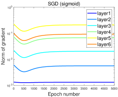
(a) Gradient vanishing of SGD

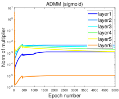
(b) Saturation-avoidance of ADMM

Figure 4: Gradient vanishing of SGD and saturation-avoidance of ADMM in the training of deep sigmoid nets. The numerical setting is the same as that of Figure 2.

3.4 Convergence of ADMM for deep sigmoid nets

Without loss of generality, we assume that $X,Y$ and $\{W_{i}^{0}\}_{i=1}^{N}$ are normalized with $\|X\|_{F}=1$, $\|Y\|_{F}=1$ and $\|W_{i}^{0}\|_{F}=1$, $i=1,\ldots,N$, and all numbers of hidden layers are the same, i.e., $d_{i}=d,\ \forall i=1,\ldots,N-1$. Under these settings, we present the main convergence theorem of ADMM in the following, while that of ADMM under more general settings is presented in Theorem 7 in Appendix B.

Theorem 4

Let $\{\c{Q}^{k}:=(\{W_{i}^{k}\}_{i=1}^{N},\{V_{i}^{k}\}_{i=1}^{N},\{\Lambda_{i}^{k}\}_{i=1}^{N})\}$ be a sequence generated by Algorithm 1. If $2\leq N\leq\sqrt{n}$, $\lambda\geq\tilde{c}N^{\frac{N-3}{2}}(nd)^{\frac{N}{2}-\frac{1}{4}}$ and $\{\beta_{i}\}_{i=1}^{N}$ satisfy

$$\beta_{N}\geq 3.5,\ \beta_{N-1}\geq 16\beta_{N},\ \beta_{i}\geq\tilde{c}_{1}\beta_{N-1}(Nnd)^{\frac{N-1-i}{2}},\ i=1,\ldots,N-2$$ (23)

for some constants $\tilde{c},\tilde{c}_{1}>0$ independent of $n,N$, then we have:

1. the augmented Lagrangian sequence $\{{\cal L}({\cal Q}^{k})\}$ is convergent.

2. $\{{\cal Q}^{k}\}$ converges to a stationary point ${\cal Q}^{*}:=(\{W_{i}^{*}\}_{i=1}^{N},\{V_{i}^{*}\}_{i=1}^{N},\{\Lambda_{i}^{*}\}_{i=1}^{N})$ of the augmented Lagrangian ${\cal L}$, which is also a KKT point (defined in(3.4) below) of problem (5), implying that $\{W_{i}^{*}\}_{i=1}^{N}$ is a stationary point of problem (4) with $\lambda^{\prime}=2\lambda/n$.

3. $\frac{1}{K}\sum_{k=1}^{K}\|\nabla{\cal L}({\cal Q}^{k})\|_{F}^{2}\rightarrow 0$ at a rate of order ${\cal O}(\frac{1}{K})$.

Theorem 4 establishes the global convergence of ADMM to a KKT point at a rate of ${\cal O}(1/K)$. By (23), the parameters $\{\beta_{i}\}_{i=1}^{N}$ increase exponentially fast from the output layer to the input layer. Moreover, by Theorem 4, the regularization parameter $\lambda$ is also required to grow exponentially fast as the depth increases. Back to the original DNN training model (4), the requirement on the regularization parameter $\lambda^{\prime}$ is $\lambda^{\prime}\geq\tilde{c}N^{\frac{N-3}{2}}d^{\frac{N}{2}-\frac{1}{4}}n^{\frac{N}{2}-\frac{5}{4}}$. Particularly, when $N=2$, namely, the neural networks with single hidden layer, then $\lambda^{\prime}=\tilde{c}\sqrt[4]{d^{3}/n}$ is a good choice, which implies that the regularization parameter can be small when the sample size $n$ is sufficiently large. Despite these convergence conditions seem a little stringent, by the existing literature (Chui et al., 2018, 2019), the depth of deep sigmoid nets is usually small, say, 2 or 3 for realizing some important data features in deep learning. Moreover, as shown in the numerical results to be presented in Sections 5 and 6, a moderately large augmented Lagrangian parameter (say, each $\beta_{i}=1$) and a small regularization parameter (say, $\lambda=10^{-6}$) are empirically enough for the proposed ADMM. In this case, the KKT point found by ADMM should be close to the optimal solutions to the empirical risk minimization of DNN training.

Remark 1: KKT conditions. Based on (6), the Karush-Kuhn-Tucker (KKT) conditions of the problem (5) can be derived as follows. Specifically, let $\{W_{i},V_{i}\}_{i=1}^{N}$ be an optimal solution of problem (5), then there exit multipliers $\{\Lambda_{i}\}_{i=1}^{N}$ such that the following hold:

$$0=\lambda W_{1}+(\Lambda_{1}\odot\sigma^{\prime}(W_{1}V_{0}))V_{0}^{T},$$

$$0=\lambda W_{i}+(\Lambda_{i}\odot\sigma^{\prime}(W_{i}V_{i-1}))V_{i-1}^{T},\ i=2,\ldots,N-1,$$

$$0=\lambda W_{N}+\Lambda_{N}V_{N-1}^{T},$$

$$0=-\Lambda_{i}+W_{i+1}^{T}(\Lambda_{i+1}\odot\sigma^{\prime}(W_{i+1}V_{i})),\ i=1,\ldots,N-2,$$ (24)

$$0=-\Lambda_{N-1}+W_{N}^{T}\Lambda_{N},$$

$$0=-\Lambda_{N}+(V_{N}-Y),$$

$$0=\sigma(W_{i}V_{i-1})-V_{i},\ i=1,\ldots,N-1,$$

$$0=W_{N}V_{N-1}-V_{N}$$

where $V_{0}=X$. From (3.4), the KKT point of problem (5) exactly fits these nonlinear constraints. Moreover, given a KKT point $(\{W_{i}^{*}\}_{i=1}^{N},\{V_{i}^{*}\}_{i=1}^{N},\{\Lambda_{i}^{*}\}_{i=1}^{N})$ of (5), substituting the last five equations into the first three equations of (3.4) shows that $\{W_{i}^{*}\}_{i=1}^{N}$ is also a stationary point of the original DNN training model (4).

Remark 2: More general activations: As presented in Theorem 7 in Appendix B, the convergence results in Theorem 4 still hold for a general class of smooth activations such as the hyperbolic tangent activation as studied in (Lin et al., 2019). Actually, the approximation result yielded in Theorem 3 can be also easily extended to a class of twice differentiable sigmoid-type activations.

4 Related Work and Discussions

In this section, we present some related works and show the novelty of our studies.

4.1 Deep sigmoid nets versus deep ReLU nets in approximation

Deep ReLU nets are the most popular neural networks in deep learning. Compared with deep sigmoid nets, there are commonly three advantages of deep ReLU nets (Nair and Hinton, 2010). At first, the piecewise linear property makes it easy to compute the derivative to ease the training via gradient-type algorithms. Then, the derivative of ReLU is either $1$ or $0$, which in a large extent alleviates the saturation phenomenon for deep sigmoid nets and particularly the gradient vanishing/explotion issue of the gradient-descent based algorithms for the training of deep neural networks. Finally, $\sigma_{relu}(t)=0$ for $t<0$ enables the sparseness of the neural networks, which coincides with the biological mechanism for neural systems.

Theoretical verification for the power of depth in deep ReLU nets is a hot topic in deep learning theory. It stems from the study in (Eldan and Shamir, 2016), where some functions were constructed to be well approximated by deep ReLU nets but cannot be expressed by shallow ReLU nets with similar number of parameters. Then, numerous interesting results on the expressivity and generalization of deep ReLU nets have been provided in (Yarotsky, 2017; Safran and Shamir, 2017; Shaham et al., 2018; Petersen and Voigtlaender, 2018; Schwab and Zech, 2019; Guo et al., ; Zhou, 2018, 2020; Chui et al., 2020; Han et al., 2020). Typically, it was proved in (Yarotsky, 2017) that deep ReLU nets perform at least not worse than the classical linear approaches in approximating smooth functions, and are beyond the capability of shallow ReLU nets. Furthermore, it was also exhibited in (Shaham et al., 2018) that deep ReLU nets can extract the manifold structure of the input space and the smoothness of the target functions simultaneously.

The problem is, however, that there are frequently too many hidden layers for deep ReLU nets to extract data features. Even for approximating the extremely simple square function, Lemma 1 requires $\log(\varepsilon^{-1})$ depth, which is totally different from deep sigmoid nets. Due to its infinitely differentiable property, sigmoid function is the most popular activation for shallow nets (Pinkus, 1999). The universal approximation property of shallow sigmoid nets has been verified in (Cybenko, 1989) for thirty years. Furthermore, (Mhaskar, 1993, 1996) showed that the approximation capability of shallow sigmoid nets is at least not worse than that of polynomials. However, there are also several bottlenecks for shallow sigmoid nets in embodying the locality (Chui et al., 1994), extracting the rotation-invariance (Chui et al., 2019) and producing sparse estimators (Lin et al., 2017), which show the necessity to deepen the neural networks. Different from deep ReLU nets, adding only a few hidden layers can significantly improve the approximation capability of shallow sigmoid nets. In particular, deep sigmoid nets with two hidden layers are capable of providing localized approximation (Chui et al., 1994), reflecting the spatially sparseness (Lin, 2019) and embodying the rotation-invariance (Chui et al., 2019).

In a nutshell, as shown in Table 1, it was proved in the existing literature that any function expressible for deep ReLU nets can also be well approximated by deep sigmoid nets with fewer hidden layers and free parameters. Our Theorem 3 partly reveals the reason for such a phenomenon in the sense that ReLU can be well approximated by sigmoid nets but not vice-verse.

4.2 Algorithms for DNN training

In order to address the choice of learning rate in SGD, there are many variants of SGD incorporated with adaptive learning rates called adaptive gradient methods. Some important adaptive gradient methods are Adagrad (Duchi et al., 2011), Adadelta (Zeiler, 2012), RMSprop (Tieleman and Hinton, 2012), Adam (Kingma and Ba, 2015), and AMSGrad (Reddi et al., 2018). Although these adaptive gradient methods have been widely used in deep learning, there are few theoretical guarantees when applied to the deep neural network training, a highly nonconvex and possibly nonsmooth optimization problem (Wu et al., 2019). Regardless the lack of theoretical guarantees of the existing variants of SGD, another major flaw is that they may suffer from the issue of gradient explosion/vanishing (Goodfellow et al., 2016), essentially due to the use of BackProp (Rumelhart et al., 1986) for updating the gradient during the iteration procedure.

To address the issue of gradient vanishing, there are some tricks that focus on either the design of the network architectures such as ResNets (He et al., 2016) or the training procedure such as the batch normalization (Ioffe and Szegedy, 2015) and weight normalization (Salimans and Kingma, 2016). Besides these tricks, there are many works in the perspective of algorithm design, aiming to propose some alternatives of SGD to alleviate the issue of gradient vanishing. Among these alternatives, the so called gradient-free type methods have recently attracted rising attention in deep learning since they may in principle alleviate this issue by their gradient-free natures, where the alternating direction method of multipliers (ADMM) and block coordinate descent (BCD) methods are two most popular ones (see, (Carreira-Perpinan and Wang, 2014; Taylor et al., 2016; Kiaee et al., 2016; Yang et al., 2016; Murdock et al., 2018; Gotmare et al., 2018; Zhang and Brand, 2017; Gu et al., 2018; Lau et al., 2018; Zeng et al., 2019)). Besides the gradient-free nature, another advantage of both ADMM and BCD is that they can be easily implemented in a distributed and parallel manner, and thus are capable of solving distributed/decentralized large-scale problems (Boyd et al., 2011).

In the perspective of constrained optimization, all the BackProp (BP), BCD and ADMM can be regarded as certain Lagrangian methods or variants for the nonlinearly constrained formulation of DNN training problem. In (LeCun, 1988), BP was firstly reformulated as a Lagrangian multiplier method. The fitting of nonlinear equations motivated by the forward pass of the neural networks plays a central role in the development of BP. Following the Lagrangian framework, the BCD methods for DNN training proposed by (Zhang and Brand, 2017; Lau et al., 2018; Zeng et al., 2019; Gu et al., 2018) can be regarded as certain Lagrangian relaxation methods without requiring the exact fitting of nonlinear constraints. Unlike in BP, such nonlinear constraints are directly lifted as quadratic penalties to the objective function in BCD, rather than involving these nonlinear constraints with Lagrangian multipliers. However, such a lifted treatment of nonlinear constraints in BCD as penalties suffers from an inconsistent issue in the sense that the solution found by BCD cannot converge to a solution satisfying these nonlinear constraints. To tackle this issue, ADMM, a primal-dual method based on the augmented Lagrangian by introducing the nonlinear constraints via Lagrangian multipliers, enables a convergent sequence satisfying the nonlinear constraints. Therefore, ADMM attracted rising attention in deep learning with various implementations (Carreira-Perpinan and Wang, 2014; Taylor et al., 2016; Kiaee et al., 2016; Yang et al., 2016; Gotmare et al., 2018; Murdock et al., 2018). However, most of the existing ADMM type methods in deep learning only keep partial nonlinear constraints for the sake of reducing the difficulty of optimization, and there are few convergence guarantees (Gao et al., 2020).

4.3 Convergence of ADMM and challenges

Most results in the literature on the convergence of nonconvex ADMM focused on linear constrained optimization problems (e.g. (Hong et al., 2016; Wang et al., 2019)). Following the similar analysis of (Wang et al., 2019), (Gao et al., 2020) extended the convergence results of ADMM to multiaffine constrained optimization problems. In the analysis of (Hong et al., 2016; Wang et al., 2019; Gao et al., 2020), the separation of a special block of variables is crucial for the convergence of ADMM in both linear and multiaffine scenarios. Following the notations of (Wang et al., 2019), the linear constraint considered in (Wang et al., 2019) is of the form

$${\bf A}{\bf x}+B{y}=0$$ (25)

where ${\bf x}:=(x_{0},\ldots,x_{p})$ includes $p+1$ blocks of variables, $y$ is a special block of variables, ${\bf A}:=[A_{0},\ldots,A_{p}]$ and $B$ are two matrices satisfying ${\mathrm{Im}({\bf A})\subseteq\mathrm{Im}(B)}$, where $\mathrm{Im}(\cdot)$ returns the image of a matrix. Similarly, (Gao et al., 2020) extended (25) to multiaffine constraint of the form, ${\cal A}(x_{1},x_{2})+{\cal B}(y)=0,$ where ${\cal A}$ and ${\cal B}$ are respectively some multiaffine and linear maps satisfying ${\mathrm{Im}({\cal A})\subseteq\mathrm{Im}({\cal B})}$. Leveraging this special block variable $y$, the dual variables (namely, multipliers) is expressed solely by $y$ (Wang et al., 2019, Lemma 3), and the amount of dual ascent part is controlled by the amount of descent part brought by the primal $y$-block update (Wang et al., 2019, Lemma 5). Together with the descent quantity arisen by the ${\bf x}$-block update, the total progress of one step ADMM update is descent along the augmented Lagrangian. Such a technique is in the core of analysis in (Wang et al., 2019) and (Gao et al., 2020) to deal with some multiaffine constraints in deep learning.

However, in a general formulation of ADMM for DNN training (e.g. (5)), it is impossible to separate such a special variable block ${y}$ satisfying these requirements. Let us take a three-layer neural network for example. Let ${\cal W}:=\{W_{i}\}_{i=1}^{3}$ be the weight matrices of the neural network, and ${\cal V}:=\{V_{i}\}_{i=1}^{3}$ be the response matrices of the neural network and $X$ be the input matrix, then the nonlinear constraints are of the following form,

$$\sigma(W_{1}X)-V_{1} =0,$$ (26a)

$$\sigma(W_{2}V_{1})-V_{2} =0,$$ (26b)

$$W_{3}V_{2}-V_{3} =0,$$ (26c)

where $\sigma$ is the sigmoid activation. Note that in (26b) and (26c), $W_{2}$ is coupled with $V_{1}$ and $W_{3}$ is coupled with $V_{2}$, respectively, so none of these four variable blocks can be separated from the others. Although $W_{1}$ in (26a) and $V_{3}$ in (26c) can be separated, the image inclusion constraint above is not satisfied. Therefore, one cannot exploit the structure in (Wang et al., 2019; Gao et al., 2020) to study such constraints in deep learning.

4.4 Key stones to the challenges and main idea of proof

In order to address the challenge of such nonlinear constraints $\sigma(W_{i}V_{i-1})-V_{i}=0$, we introduce a local linear approximation (LLA) technique. Let us take (26) for example to illustrate this idea. The most difficult block of variable is $V_{1}$ which involves two constraints, namely, a linear constraint in (26a), and a nonlinear constraint in (26b). Now we fix $W_{1},W_{2}$ and $V_{2}$ as the previous updates, say $W_{1}^{0},W_{2}^{0}$ and $V_{2}^{0}$, respectively. For the update of $V_{1}$-block, we keep the linear constraint, but relax the nonlinear constraint with its linear approximation at the previous update $V_{1}^{0}$,

$$\sigma(W_{2}^{0}V_{1}^{0})-V_{2}^{0}+\sigma^{\prime}(W_{2}^{0}V_{1}^{0})\odot\left[W_{2}^{0}(V_{1}-V_{1}^{0})\right]\approx 0,$$ (27)

assuming the differentiability of activation function $\sigma$. The other blocks can be handled in a similar way. Taking $W_{1}$ block for example, we relax the related nonlinear constraint via its linear approximation at the previous update $W_{1}^{0}$, namely, $\sigma(W_{1}^{0}X)-V_{1}^{0}+\sigma^{\prime}(W_{1}^{0}X)\odot((W_{1}-W_{1}^{0})X)\approx 0.$ The operations of LLA on the nonlinear constraints can be regarded as applying certain prox-linear updates (Xu and Yin, 2013) to replace the subproblems of ADMM involving nonlinear constraints as shown in Section 3.2.

To make such a local linear approximation valid, intuitively one needs: (a) the activation function $\sigma$ is smooth enough; and (b) the linear approximation occurs in a small enough neighbourhood around the previous updates. Condition (a) is mild and naturally satisfied by the sigmoid type activations. But condition (b) requires us to introduce a new Lyapunov function defined in (29) by adding to the original augmented Lagrangian a proximal control between $V_{i}$ and its previous updates. Equipped with such a Lyapunov function, we are able to show that an auxiliary sequence converges to a stationary point of the new Lyapunov function (see Theorem 5 below), which leads to the convergence of the original sequence generated by ADMM (see Theorem 4 in Section 3.4). Specifically, denote $\{{\hat{\cal Q}}^{k}\}$ as

$${\hat{\cal Q}}^{k}:=({\cal Q}^{k},\{\hat{V}_{i}^{k}\}_{i=1}^{N}),$$ (28)

with $\hat{V}_{i}^{k}:=V_{i}^{k-1}$ for $i=1,\ldots,N$ and $k\geq 1$, and $\hat{\cal L}({\hat{\cal Q}}^{k})$ as

$$\hat{\cal L}({\hat{\cal Q}}^{k}):={\cal L}({\cal Q}^{k})+\sum_{i=1}^{N}\xi_{i}\|V_{i}^{k}-\hat{V}^{k}_{i}\|_{F}^{2}$$ (29)

for some positive constant $\xi_{i}>0$ ($i=1,\ldots,N$) specified later in Appendix D.1.4. Then we state the convergence of $\{{\hat{\cal Q}}^{k}\}$ as follows.

Theorem 5 (Convergence of $\{{\hat{\cal Q}}^{k}\}$)

Under conditions of Theorem 4, we have:

1. $\hat{\cal L}({\hat{\cal Q}}^{k})$ is convergent.

2. ${\hat{\cal Q}}^{k}$ converges to some stationary point ${\hat{\cal Q}}^{*}$ of $\hat{\cal L}$.

3. $\frac{1}{K}\sum_{k=1}^{K}\|\nabla\hat{\cal L}({\hat{\cal Q}}^{k})\|_{F}^{2}\rightarrow 0$ at a ${\cal O}(\frac{1}{K})$ rate.

Theorem 5 presents the function value convergence and sequence convergence to a stationary point at a ${\cal O}(1/K)$ rate of the auxiliary sequence $\{{\hat{\cal Q}}^{k}\}$. By the definitions (28) and (29) of ${\hat{\cal Q}}^{k}$ and $\hat{\cal L}$ , Theorem 5 directly implies Theorem 4. As shown by the proofs in Appendix D, the claims in Theorem 5 also hold under the more general assumptions for Theorem 7 in Appendix B. In Theorem 5, we only give the convergence guarantee for the proposed ADMM. It would be interesting to derive the convergence rate to highlight the role of algorithmic parameters. We will keep in study and report the result in future work.

Our main idea of proof for Theorem 5 can be summarized as follows: we firstly establish a sufficient descent lemma along the new Lyapunov function (see Lemma 14 in Section D.1), then show a relative error lemma (see Lemma 21 in Section D.1.5), and later verify the Kurdyka-Łojasiewicz property (Łojasiewicz, 1993; Kurdyka, 1998) (see Lemma 13 in Section C.2) and the limiting continuity property of the new Lyapunov function by Assumption 1, and finally establish Theorem 5 via following the analysis framework formulated in (Attouch et al., 2013, Theorem 2.9). In order to prove Lemma 14, we prove the following three lemmas, namely, a one-step progress lemma (see Lemma 15 in Section D.1.1), a dual-bounded-by-primal lemma (see Lemma 18 in Section D.1.2), and a boundedness lemma (see Lemma 19 in Section D.1.3), while to prove Lemma 21, besides Lemmas 18 and 19, we also use the Lipschitz continuity of the activation and its derivative by Assumption 1 in Appendix B. The proof sketch can be illustrated by Figure 5.

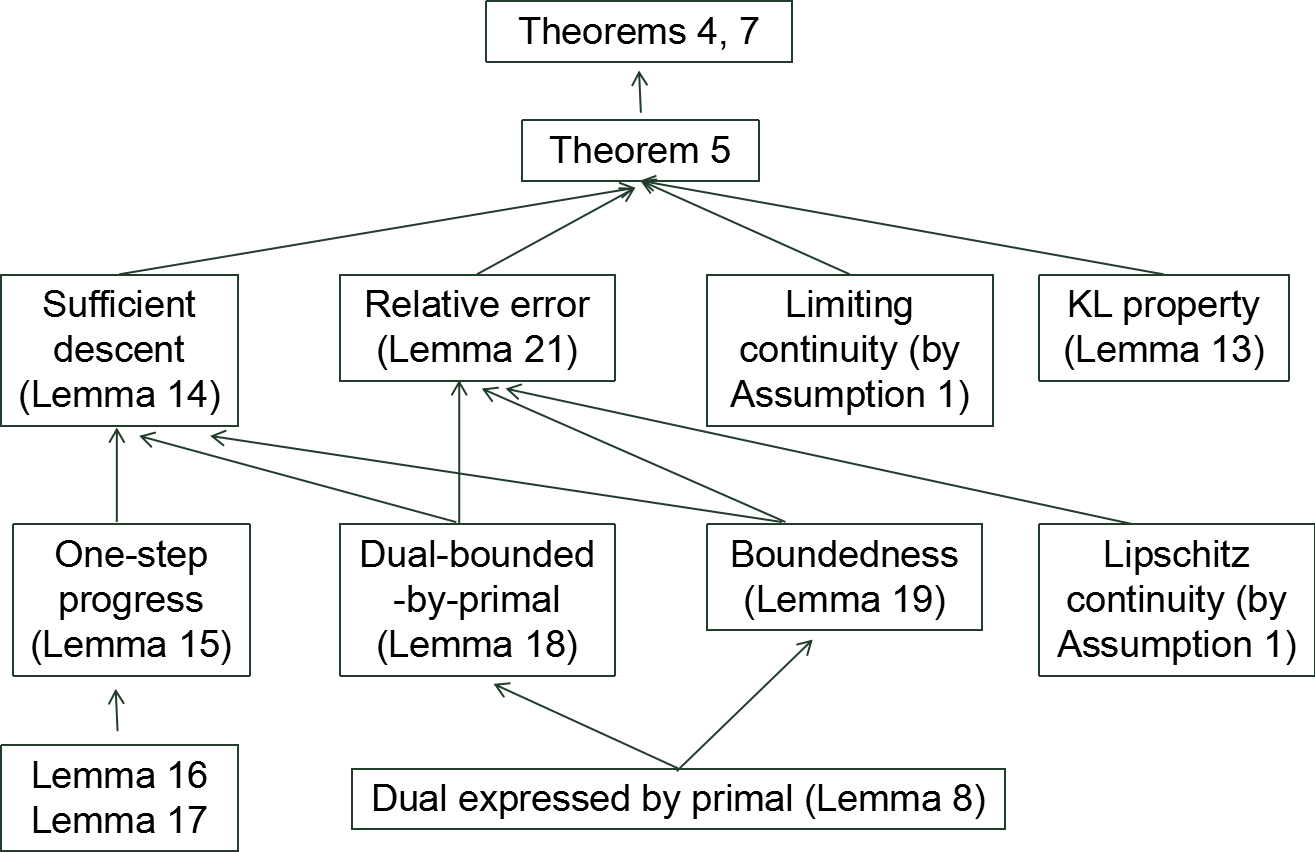
Figure 5: Proof sketch of convergence of ADMM.

According to Figure 5, we show the boundedness of the sequence before the establishment of the sufficient descent lemma (i.e., Lemma 14). Such a proof procedure is different from the existing ones in the literature (say, (Wang et al., 2019)), where a sequence boundedness is usually implied by firstly showing the (sufficient) descent lemma (Wang et al., 2019, Lemma 6).

5 Toy Simulations

In this section, we conduct a series of simulations to show the effectiveness of the proposed ADMM in approximating and learning some natural functions including the square function, product gate, a piecewise $L_{1}$ radial function, and a smooth $L_{2}$ radial function, which play important roles in reflecting some commonly used data features (Safran and Shamir, 2017; Shaham et al., 2018; Chui et al., 2019; Guo et al., ). In particular, we provide empirical studies to show that these important natural functions can be numerically well approximated or learned by the proposed ADMM-sigmoid pair. Furthermore we also show that the proposed ADMM-sigmoid pair is stable to its algorithmic hyper-parameters, via comparing to the popular deep learning optimizers including the vanilla SGD, SGD with momentum (called SGDM for short henceforth) and Adam (Kingma and Ba, 2015). There are four experiments concerning approximation and learning tasks: (a) approximation of square function, (b) approximation of product gate, (c) learning of a piecewise $L_{1}$ radial function, and (d) learning of a smooth $L_{2}$ radial function. All numerical experiments were carried out in Matlab R2015b environment running Windows 10, Intel(R) Xeon(R) CPU E5-2667 v3 @ 3.2GHz 3.2GH. The codes are available at https://github.com/JinshanZeng/ADMM-DeepLearning.

5.1 Experimental settings

In all our experiments, we use deep fully connected neural networks with different depths and widths. Throughout the paper, the depth and width of deep neural networks are respectively the number of hidden layers and number of neurons in each hidden layer. For simplicity, we only consider deep neural networks with the same width for all the hidden layers. We consider both deep sigmoid nets and deep ReLU nets in the simulation. Motivated by the existing literature (Guo et al., ), the depth required for deep ReLU nets is in general much more than that for deep sigmoid nets in the aforementioned approximation or learning tasks. For the fairness of comparison, we consider deep ReLU nets with more hidden layers, i.e., the maximal depth of deep ReLU nets is 20 while that of deep sigmoid nets is only 5 or 6, as presented in Table 2. Besides the vanilla SGD-ReLU pair (SGD (ReLU) for short), we also consider SGD-sigmoid pair (SGD (sigmoid) for short), SGDM-ReLU pair (SGDM (ReLU) for short), and Adam-ReLU pair (Adam (ReLU) for short) as the competitors. Similarly, we denote by ADMM (sigmoid) the proposed ADMM-sigmoid pair.

For each experiment, our purposes are mainly two folds: excellent approximation or learning performance, and stability with respect to initialization schemes and penalty parameters with appropriate neural network structures for the proposed ADMM-sigmoid pair. For the first purpose, we consider deep neural networks with different depths and widths as presented in Table 2. Moreover, for ADMM, we empirically set the regularization parameter $\lambda=10^{-6}$ and the augmented Lagrangian parameters $\beta_{i}$’s as the same $1$, while for SGD methods, we empirically utilize the step exponential decay (or, called geometric decay) learning rate schedule with the decay exponent $0.95$ for every 10 epochs. For SGDM and Adam, we use the default settings as presented in Table 2. The number of epochs in all experiments is empirically set as 2000. The specific settings of these experiments are presented in Table 2.

Table 2: Experimental settings for toy simulations. Sample sizes for approximation tasks are set as 1000, and training and test samples sizes for learning tasks are set as 1000 respectively. The notation $[a:b]$ is denoted by the set $\{a,a+1,\ldots,b\}$ for two integers $a,b$. ${\dagger}$ In the case of learning the $L_{2}$ radial function, ranges of depth of deep sigmoid and ReLU nets are $[2,6]$ and $[2,20]$, respectively.

task	functions	deep fully-connected NNs		SGDs (sigmoid/ReLU), SGDM		SGDM	Adam	ADMM
		width	depth	learning rate (lr)	batch size	(momentum)		$(\lambda,\beta)$
Approx.	$x^{2}$	$20\times[1:5]$	$[1,5]$ (sigmoid),				lr: 0.001
	$uv$	$60\times[1:5]$	$[1,20]$ (ReLU)	$0.1\times 0.95^{k}$	50	0.5	$\beta_{1}$: 0.9	$(10^{-6},1)$
Learn.	$(\|x\|_{1}-1)_{+}$	$10\times[1:6]$		per 10 epochs,			$\beta_{2}$: 0.999
	$g(|x|^{2})$	$100\times[1:5]$	$[2,6]$, $[2,20]$ †				$\epsilon$: 1e-8

For the second purpose, we consider different regularization and penalty parameters $(\lambda\in\{10^{-6},10^{-5},10^{-4},10^{-3},10^{-2},10^{-1}\},\beta\in\{0.01,0.1,0.5,1,5,10,100\})$, as well as several existing initialization schemes for ADMM under the optimal neural network structure determined by the first part. Particularly, we consider the following four types of schemes yielding six typical initializations:

1. LeCun random initialization (LeCun et al., 1998): the components of the weight matrix $W_{l}$ at the $l$-th layer are generated i.i.d. according to some random distribution with zero mean and variance $\frac{1}{d_{l-1}}$, $l=1,\ldots,N$. Particularly, we consider two special LeCun random initialization schemes generated respectively according to the uniform and Gaussian distributions, i.e., $W_{l}\sim U([-\sqrt{\frac{3}{d_{l-1}}},\sqrt{\frac{3}{d_{l-1}}}])$ (LeCun-Unif for short) and $W_{l}\sim{\cal N}(0,\frac{1}{d_{l-1}})$ (LeCun-Gauss for short).

2. Random orthogonal initialization (Saxe et al., 2014): the weight matrix $W$ is set as some random orthogonal matrix such that $W^{T}W={\bf I}$ or $WW^{T}={\bf I}$. We call it Orth-Unif (or Orth-Gauss) for short if the random matrix is generated i.i.d. according to the uniform random (or, Gaussian) distribution.

3. Xavier initialization (Glorot and Bengio, 2010): each $W_{l}\sim U([-\sqrt{\frac{6}{d_{l-1}+d_{l}}},\sqrt{\frac{6}{d_{l-1}+d_{l}}}])$, $l=1,\ldots,N$.

4. MSRA initialization (He et al., 2015): $W_{l}\sim{\cal N}(0,\frac{2}{d_{l}})$, $l=1,\ldots,N-1$, and $W_{N}\sim{\cal N}(0,\frac{1}{d_{N}})$ since there is no ReLU activation for the last layer.

The default settings for initial threshold vectors in the above initialization schemes are set to be 0. For each group of parameters, we run 20 trails for average. Specifically, for the approximation tasks, the performance of an algorithm is measured by the approximation error, defined as the average of these 20 trails’s mean square errors, while for the learning tasks, the performance of an algorithm is measured by the test error, defined as the average of the mean square errors of these trails over the test data.

5.2 Approximation of square function

In these experiments, we consider the performance of the ADMM-sigmoid pair in approximating the univariate square function, that is, $f(x)=x^{2}$ on $[-1,1]$. The specific experimental settings can be found in Table 2.

A. Approximation performance of ADMM. Experiment results over the best neural network structures are presented in Table 3, and trends of approximation errors with respect to the depth are shown in Figure 6. From Table 3, the ADMM-SGD pair can approximate the square function within very high precision, i.e., in the order of $10^{-9}$, which is slightly better than that of competitors for deeper ReLU nets, and is much better than the SGD-sigmoid pair with the same depth. Specifically, optimal depths for SGD (ReLU), SGDM (ReLU) and Adam (ReLU) are 18, 15, 15, respectively, while the optimal depth for ADMM (sigmoid) is only 2, which matches the theoretical results in approximation theory, as shown in (Chui et al., 2019, Proposition 2). In terms of running time, ADMM (sigmoid) with optimal network structures is generally faster than the SGDM (ReLU) and Adam (ReLU) with optimal network structures as presented in the third row of Table 3, mainly due to the depth required for ADMM (sigmoid) is much less than those for deep ReLU nets SGD (ReLU), SGDM (ReLU) and Adam (ReLU). Moreover, according to Figure 6, ADMM (sigmoid) can yield high approximation precision with less layers than the competitors. These experimental results demonstrate that the proposed ADMM can embody the advantage of deep sigmoid nets on approximating the square function, as pointed out in the existing theoretical literature (Chui et al., 2019).

Table 3: Experimental results of different algorithms in approximating $f(x)=x^{2}$. The standard derivation of the approximation error is presented in the parentheses. The running time is recorded in seconds. The depth and width of the optimal network structure in terms of approximation error is presented in the last row.

Algorithm	SGD (ReLU)	SGDM (ReLU)	Adam (ReLU)	SGD (sigmoid)	ADMM (sigmoid)
Approx. Error	5.34e-8(2.34e-8)	3.95e-8(1.25e-8)	3.33e-8(1.46e-8)	2.46e-4(1.69e-4)	2.53e-9(1.18e-9)
Run Time (s)	26.99	41.35	38.26	3.45	9.47
(depth, width)	(18,100)	(15,100)	(15,80)	(2,60)	(2,100)

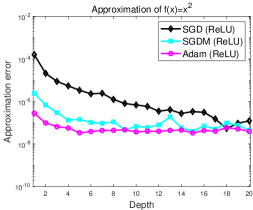
(a) Deep ReLU nets

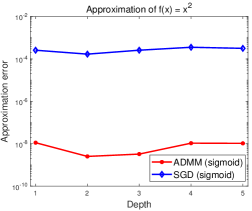
(b) Deep sigmoid nets

Figure 6: Effect of the depth of neural networks in approximating the square function.

B. Effect of parameters for ADMM. There are mainly two parameters for the proposed ADMM, i.e., the model parameter $\lambda$ (also called as the regularization parameter) and the algorithm parameter $\beta$ involved in the augmented Lagrangian (also called as the penalty parameter). In this experiment, we consider the performance of ADMM in approximating the univariate square function with different model and algorithmic parameters, under the optimal neural networks, i.e., deep fully-connected neural networks with depth 2 and width 100. Specifically, the regularization and penalty parameters vary from $\{10^{-6},10^{-5},10^{-4},10^{-3},10^{-2},10^{-1}\}$ and $\{0.01,0.1,0.5,1,5,10,100\}$, respectively. The approximation errors of ADMM with these parameters are shown in Figure 7(a). From Figure 7(a), considering the penalty parameter $\beta$, ADMM with $\beta=1$ achieves the best performance in most cases, as also observed in the experiments later. Thus, in practice, we can empirically set the penalty parameter $\beta$ as $1$. Since $\lambda$ is a model parameter, it usually has significant effect on the performance of the proposed ADMM. From Figure 7(a), a small regularization parameter (say, $\lambda=10^{-6}$) is sufficient to yield an ADMM solver with high approximation precision.

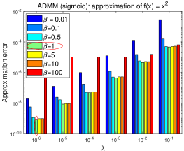
(a) Effect of parameters of ADMM

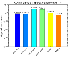
(b) Stability of initialization

Figure 7: Effect of parameters for ADMM in approximating the univariate square function.

C. Effect of initial schemes. Besides the MSRA initialization (He et al., 2015), there are some other commonly used initial schemes such as the random orthogonal initializations (Saxe et al., 2014), LeCun random initializations (LeCun et al., 1998), and Xavier initialization (Glorot and Bengio, 2010). Under the optimal parameter settings presented in Table 3, the performance of the ADMM-sigmoid pair with different initialization schemes is presented in Figure 7(b). From Figure 7(b), the proposed ADMM performs well for all the initialization schemes. This demonstrates that the proposed ADMM is stable to the initial scheme.

5.3 Approximation of product gate

In this subsection, we present experimental results in approximating the product gate function, i.e., $f(u,v)=uv$ for $u,v\in[-1,1]$. The specific experimental settings in approximating the product gate function can be found in Table 2.

A. Approximation performance of ADMM. The performance of ADMM and competitors is presented in Table 4, and their performance with respect to the depth is depicted in Figure 8. From Table 4, the product gate function can be well approximated by the ADMM-sigmoid pair with precision in the order of $10^{-9}$, which is better than those of competitors including SGD (ReLU), SGDM (ReLU) and Adam (ReLU), even when more hidden layers are involved in the training. It follows from Figure 8(b) and Table 4 that the optimal depth for ADMM in approximating the product gate function is $2$, which matches the theoretical depth for the approximation of product gate as shown in (Chui et al., 2019, Proposition 3). Similar to the case of approximating square function, the running time of the proposed ADMM-sigmoid pair is less than the SGD type competitors for deep ReLU nets with more hidden layers.

Table 4: Experimental results of different algorithms in approximating $f(u,v)=uv$.

Algorithm	SGD (ReLU)	SGDM (ReLU)	Adam (ReLU)	SGD (sigmoid)	ADMM (sigmoid)
Approx. Error	1.22e-6(3.68e-7)	3.37e-7(1.29e-7)	1.13e-6(4.37e-7)	1.13e-3(2.33e-4)	2.62e-9(1.05e-9)
Run Time (s)	66.37	54.17	46.58	9.72	17.29
(depth, width)	(20,300)	(18,180)	(13,120)	(2,240)	(2,300)

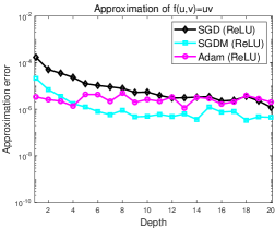
(a) Deep ReLU nets

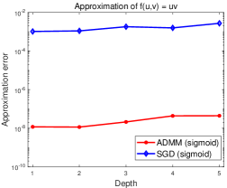
(b) Deep sigmoid nets

Figure 8: Effect of the depth of neural networks in approximating the product-gate function.

B. Effect of parameters of ADMM. Similar to Section 5.2 B, we also consider the effect of parameters $\lambda$ and $\beta$ for ADMM under the optimal network structures, which is presented in Figure 9(a). From Figure 9(a), the effect of the concerned parameters on the performance of ADMM in approximating the product gate function is very similar to that in the approximation of univariate square function. It can be observed that the settings of parameters with $(\lambda=10^{-6},\beta=1)$ are empirically good for ADMM in these two approximation tasks.

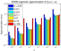
(a) Effect of parameters of ADMM

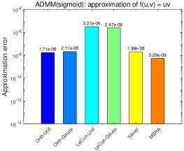
(b) Stability of initialization

Figure 9: Effect of parameters for ADMM in approximating the product-gate function.

C. Effect of initial schemes. Moreover, in this experiment, we consider the performance of ADMM (sigmoid) for the aforementioned six different initialization schemes. The experimental results are shown in Figure 9(b). It can be observed in Figure 9(b) that all the initial schemes are generally effective in yielding an ADMM solver with high precision. Among these effective initialization schemes, the LeCun type of initializations perform slightly worse than the others. This, in some extent, also implies that the proposed ADMM is usually stable to initial schemes.

5.4 Learning $L_{1}$ radial function

In this subsection, we consider the performance of the ADMM-sigmoid pair for learning a two-dimensional $L_{1}$ radial function, i.e., $f(x)=(\|x\|_{1}-1)_{+}:=\max\{0,\|x\|_{1}-1\}$ for $x\in[r,(1+\epsilon)r]\times[r,(1+\epsilon)r]$ for some $r>0$ and $\epsilon>0$. Such an $L_{1}$ radial function was particularly considered in (Safran and Shamir, 2017). In our experiments, we let $\epsilon=1/2$ and $r=1-\frac{\epsilon}{2}$ in light of the theoretical studies in (Safran and Shamir, 2017). Different from the approximation tasks in Sections 5.2 and 5.3, samples generated for the learning task include both training and test samples, where training samples are commonly generated with certain noise and the test samples are clean data. In these experiments, we consider Gaussian noises with different variances.

A. Learning performance of ADMM. Optimal test errors of different algorithms for learning the $L_{1}$ radial function are presented in Table 5, where the variance of Gaussian noise added into the training samples is $0.1$. The associated test errors of these algorithms with respect to the depth of neural networks are presented in Figure 10. From Table 5, the considered $L_{1}$ radial function can be well learned by both ADMM and SGD type methods. Specifically, the performance of the proposed ADMM is slightly better than SGD type methods. In particular, the optimal depth of deep sigmoid nets trained by ADMM is only 4, which is much less than those of deep ReLU nets trained by SGD type methods. Under optimal network structures, the running time of the suggested ADMM-pair is slightly less than that of SGD type methods for deep ReLU nets, due to the less depth of deep sigmoid nets. According to Figure 10(b), the proposed ADMM performs better than SGD for training deep sigmoid nets, and as the depth increasing, the performance of SGD gets worse possibly due to the vanishing gradient issue, while our suggested ADMM can alleviate the issue of vanishing gradient and thus achieve better and better performance in general as the depth increases in our considered range of depth, i.e., $\{1,2,3,4,5\}$.

Table 5: Performance of different algorithms for learning $L_{1}$ radial function with $0.1$ Gaussian noise.

Algorithm	SGD (ReLU)	SGDM (ReLU)	Adam (ReLU)	SGD (sigmoid)	ADMM (sigmoid)
Test Error	2.48e-5(9.74e-6)	2.26e-5(7.88e-6)	2.16e-5(8.53e-6)	4.58e-5(1.59e-5)	1.69e-5(4.34e-6)
Run Time (s)	23.24	18.23	14.66	1.68	10.36
(depth, width)	(17,50)	(13,50)	(10,50)	(1,20)	(4,10)

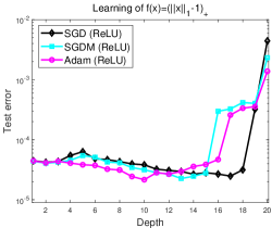
(a) Deep ReLU nets

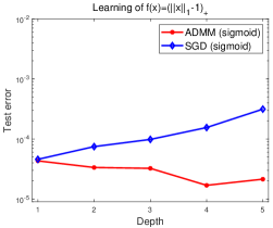
(b) Deep sigmoid nets

Figure 10: Effect of the depth of neural networks in learning the $L_{1}$ radial function.

B. Effect of parameters and initialization. Under the optimal neural network structures specified in Table 5, we consider the effect of parameters, i.e., $(\lambda,\beta)$ for ADMM, as well as the effect of the initialization schemes for both ADMM and SGD type methods. The numerical results are shown in Figure 11. From Figure 11(a), we can observe that the specific parametric setting, i.e., $\lambda=10^{-6}$ and $\beta=1$, is also empirically effective in learning $L_{1}$ radial function. By Figure 11(b), the proposed ADMM performs well for all the concerned random initialization schemes.

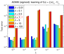
(a) Effect of parameters of ADMM

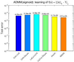
(b) Stability of initialization

Figure 11: Effect of parameters and initial schemes for ADMM in learning the $L_{1}$ radial function.

C. Robustness to the noise. Moreover, we consider the performance of the proposed ADMM for training data with different levels of noise. Specifically, under the optimal parameters specified in Table 5, we consider several levels of noise, where the variance of Gaussian noise varies from $\{0.1,0.3,\ldots,1.5\}$. Trends of training and test errors are presented in Figure 12(a) and (b) respectively. From Figure 12(a), the proposed ADMM is generally trained well in the sense that the training error almost fits the true noise level. In this case, we can observe from Figure 12(b) that the proposed ADMM is robustness to the noise in the sense that the test error increases much slower than the increasing of the variance of Gaussian noise.

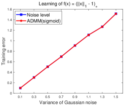
(a) Training error

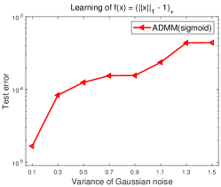
(b) Test error

Figure 12: Robustness of the proposed ADMM to the noise in learning $L_{1}$ radial function.

5.5 Learning $L_{2}$ radial function

In this subsection, we consider to learn certain smooth $L_{2}$ radial function that frequently reflects the rotation-invariance feature in deep learning (Chui et al., 2019). Specifically, we adopt a two-dimensional smooth $L_{2}$ radial function, i.e., $f(x)=g(|x|^{2})$, where $x\in[-1,1]\times[-1,1]$, $|x|^{2}:=\sum_{i=1}^{2}x_{i}^{2}$, and $g(t)=(1-t)_{+}^{5}(8t^{2}+5t+1)$ on $\mathbb{R}$ is some Wendland function (Lin et al., 2019). Except the target function $f$, the experimental settings in these experiments are similar to those in Section 5.4.

A. Learning performance of ADMM. The test error of the considered algorithms in learning such a smooth $L_{2}$ radial function is presented in Table 6, while trends of test errors with respect to the depth are shown in Figure 13. By Table 6, the considered smooth $L_{2}$ radial function can be learned by the proposed ADMM well with a small test error. Specifically, in terms of test error, the performance of the ADMM-sigmoid pair is slightly better than that of SGD type methods for deep ReLU nets, and the optimal depth of deep sigmoid nets required by ADMM is much smaller than those of deep ReLU nets required by the concerned SGD type methods. Due to less depth, the running time of ADMM is less than that of the concerned SGD type methods for deep ReLU nets under the optimal settings of neural networks. Moreover, from Figure 13(a), a deeper ReLU network with about 10 layers is generally required to learn the $L_{2}$ radial function with a good test error, while from Figure 13(b), the depth of deep sigmoid nets trained by ADMM can be much smaller (i.e., about 5) to yield a good test error.

Table 6: Test errors of different algorithms for learning $L_{2}$ radial function with $0.1$ Gaussian noise.

Algorithm	SGD (ReLU)	SGDM (ReLU)	Adam (ReLU)	SGD (sigmoid)	ADMM (sigmoid)
Test Error	1.68e-5(6.43e-6)	1.21e-5(5.25e-6)	1.02e-5(4.88e-6)	9.33e-5(1.42e-5)	9.28e-6(1.01e-6)
Run Time (s)	104.52	116.44	108.49	18.13	47.36
(depth, width)	(16,300)	(12,400)	(11,400)	(4,200)	(5,300)

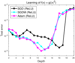
(a) Deep ReLU nets

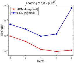
(b) Deep sigmoid nets

Figure 13: Effect of the depth of neural networks in learning the $L_{2}$ radial function.

B. Effect of parameters and initialization. In this part, we consider the effect of parameters (i.e., $\lambda$ and $\beta$) of ADMM as well as the effect of initialization for learning the $L_{2}$ radial function in the optimal settings specified in Table 6. The numerical results are presented in Figure 14. From Figure 14(a), the effect of parameters are similar to previous three simulations and it can be observed that the specific settings, i.e., $\lambda=10^{-6}$ and $\beta=1$, are empirically effective. From Figure 14, we also observe that ADMM is effective to all the random initialization schemes.

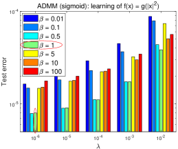
(a) Effect of parameters of ADMM

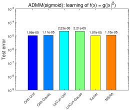
(b) Stability of initialization

Figure 14: Effect of parameters and initial schemes for ADMM in learning smooth $L_{2}$ radial function.

C. Robustness to noise. Similar to the learning of $L_{1}$ radial function, we consider the performance of the proposed ADMM for noisy training data with different levels of noise. Specifically, the variance of the Gaussian noise added into the training samples varies from $\{0.1,0.3,0.5,0.7,0.9,1.1\}$. Curves of training error and test error are shown respectively in Figure 15(a) and (b). From Figure 15, the behavior in learning $L_{2}$ radial function is similar to that in learning $L_{1}$ radial function as shown in Figure 12. This demonstrates that the proposed ADMM is also robust to noise in learning such a smooth $L_{2}$ radial function.

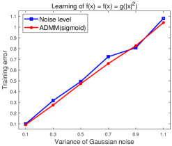
(a) Training error

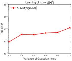
(b) Test error

Figure 15: Robustness of the proposed ADMM to the noise in learning $L_{2}$ radial function.

6 Real Data Experiments

In this section, we provide three real-data experiments over the earthquake intensity database, the extended Yale B (EYB) face recognition database and the PTB Diagnostic ECG database, to demonstrate the effectiveness of the proposed ADMM. We choose these three datasets since they can in some sense reflect certain features that can be well approximated by deep sigmoid nets, and thus, the benefits of the proposed ADMM can be embodied over these datasets. Specific experimental settings are presented in Table 7, where the penalty parameter $\beta$ is empirically set as $1$ and the regularization parameter $\lambda$ is chosen via cross validation from the set $\{10^{-6},10^{-5},10^{-4},10^{-3},10^{-2}\}$ according to the previous studies of toy simulations.

Table 7: Experimental settings for real-data experiments. The number of epochs for each case is set empirically to be 200.

dataset	(training size,	Network structure		SGDs (sigmoid/ReLU),SGDM		SGDM	Adam	ADMM
	test size)	width	depth	batch size	learning rate	(momentum)	lr:0.001	$(\lambda,\beta)$
Earthquake	(4173,4000)	$20\times[1:10]$	[1:6]	100	$0.1\times 0.95^{k}$,		$\beta_{1}$: 0.9	$\lambda\in 10^{[-6:-2]}$
EYB	(2432,2432)	$20\times[1:10]$	1	50	per 10 epochs	0.5	$\beta_{2}$: 0.999	$\beta=1$
PTB	(7000,7552)	$64\times[1:4]$	[1:10]	100			$\epsilon$: 1e-8

6.1 Earthquake intensity dataset

Earthquake Intensity Database is from: https://www.ngdc.noaa.gov/hazard/intintro.shtml. This database contains more than 157,000 reports on over 20,000 earthquakes that affected the United States from the year 1638 to 1985. For each record, the features include the geographic latitudes and longitudes of the epicentre and “reporting city” (or, locality) where the Modified Mercalli Intensity (MMI) was observed, magnitudes (as a measure of seismic energy), and the hypocentral depth (positive downward) in kilometers from the surface. The output label of each record is measured by MMI, varying from 1 to 12 in integer. An illustration of the generation procedure of each earthquake record is shown in Figure 16(a). In this paper, we transfer such multi-classification task into the binary classification since this database is very unbalanced (say, there is only one sample for the class with MMI being 1). Specifically, we set the labels lying in 1 to 4 as the positive class, while the other labels lying in 5 to 12 as the negative class, mainly according to the damage extent of the earthquake suggested by the referred website. Moreover, we removed those incomplete records with missing labels. After such preprocessing, there are total 8173 effective records, where the numbers of samples in positive and negative classes are respectively 5011 and 3162. We divide the total data set into the training and test sets randomly, where the training and test sample sizes are 4173 and 4000, respectively. Before training, we use the z-scoring normalization for each feature, that is, $\frac{x_{i}-\mu}{\sigma}$ with $\mu$ and $\sigma$ being respectively the mean and standard deviation of the $i$th feature $\{x_{i}\}$. The classification accuracies of all algorithms are shown in Table 8. The effect of the depth of neural network, algorithmic parameters, and random initial schemes are shown in Figure 16 (b)-(d) respectively.

According to Table 8, the performance of the proposed ADMM is comparable to the state-of-the-art methods in terms of test accuracy. Specifically, the proposed ADMM is slightly worse than Adam, and outperforms the other competitors in terms of test accuracy, while in terms of running time, the proposed ADMM is slightly faster than Adam and SGDM under the associated optimal network settings, mainly because the optimal depth of the deep sigmoid nets trained by ADMM is less than those of deep ReLU nets trained by Adam and SGDM. Compared to the SGD counterpart for deep sigmoid nets, the performance of the proposed ADMM is much better in terms of test accuracy. It can be observed from Figure 16(b) that the vanilla SGD may suffer from the gradient vanishing/explosion issue when training a slightly deeper sigmoid nets (say, the depth is larger than 5) due to the saturation of the sigmoid activation, while the proposed ADMM can avoid such saturation and thus alleviate the gradient vanishing/explosion issue. From Figure 16(c), the proposed ADMM with the default settings, i.e., $\lambda=$ 1e-6 and $\beta=1$ in general yields the best performance. Moreover, it can be observed from Figure 16(d) that the proposed ADMM is stable to the commonly used initialization schemes under the optimal neural network structure specified in Table 8.

Table 8: Test accuracies (%) of different algorithms for earthquake intensity database. The baseline of the test accuracy is $80.48\%$ (Zeng et al., 2020).

Algorithm	SGD (ReLU)	SGDM (ReLU)	Adam (ReLU)	SGD (sigmoid)	ADMM (sigmoid)
Test Acc(%)	81.24(0.45)	81.16(0.32)	81.31(0.36)	79.94(0.23)	81.26(0.31)
Run Time (s)	4.74	14.20	13.24	2.60	12.64
(depth, width)	(2,120)	(5,140)	(4,80)	(1,100)	(3,80)

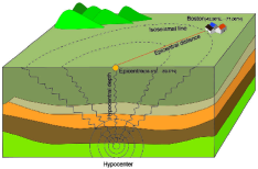
(a) An illustration of earthquake data

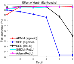
(b) Effect of depth of NNs

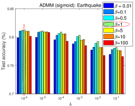
(c) Effect of parameters

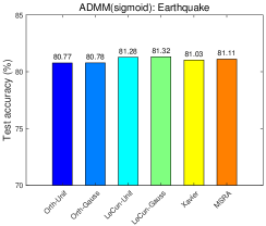
(d) Stability to initial schemes

Figure 16: Performance of ADMM in earthquake intensity data: (a) an illustration of the earthquake intensity data (Zeng et al., 2020); (b) the effect of depth of the neural network for different algorithms; (c) the effect of algorithmic parameters for the proposed ADMM; (d) the stability of the proposed ADMM to different initial schemes.

6.2 Extended Yale B face recognition database

In the extended Yale B (EYB) database, well-known face recognition database (Lee et al., 2005), there are in total 2432 images for 38 objects under 9 poses and 64 illumination conditions, where for each objective, there are 64 images. The pixel size of each image is $32\times 32$. In our experiments, we randomly divide these 64 images for each objective into two equal parts, that is, one half of images are used for training while the rest half of images are used for testing. For each image, we normalize it via the z-scoring normalization. The specific experimental settings for this database can be found in Table 7. Particularly, we empirically use a shallow neural network with depth one and various of widths, since such shallow neural network is good enough to extract the low-dimensional manifold feature of this face recognition data, as shown in Table 9. The effect of network structures and stability of the proposed ADMM to initialization schemes are shown in Figure 17(a) and (b) respectively.

According to Table 9, the proposed ADMM achieves the state-of-the-art test accuracy (see, Lu et al. (2020)) with a smaller width of the sigmoid nets when compared to the concerned competitors. From Figure 17, the proposed ADMM can achieve a very high test accuracy for most of the concerned widths of the networks and is stable to the commonly used random initial schemes.

Table 9: Performance of different algorithms for extended Yale B database. The baseline of the test accuracy is about $96\%$ in (Lu et al., 2020).

Algorithm	SGD (ReLU)	SGDM (ReLU)	Adam (ReLU)	SGD (sigmoid)	ADMM (sigmoid)
Test Acc(%)	98.84(0.28)	97.18(0.28)	98.91(0.34)	98.67(0.41)	98.93(0.43)
Run Time (s)	19.78	23.99	48.92	16.95	21.36
(depth, width)	(1,200)	(1,200)	(1,200)	(1,140)	(1,60)

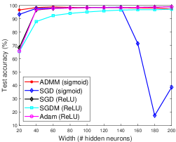
(a) Effect of network structure.

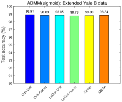
(b) Stability to initial schemes of ADMM

Figure 17: Performance of ADMM in extended Yale B database: (a) the effect of width for different algorithms; (b) the stability of the proposed ADMM to different random initial schemes.

6.3 PTB Diagnostic ECG database

An ECG is a 1D signal which is the result of recording the electrical activity of the heart using an electrode. It is one of popular tools that cardiologists use to diagnose heart anomalies and diseases. The PTB diagnostic ECG database is available at https://github.com/CVxTz/ECG_Heartbeat_Classification and was preprocessed by (Kachuee et al., 2018). There are 14,552 samples in total with 2 categories. The specific experimental settings for this database can be found in Table 7. The experiment results of the proposed ADMM and concerned competitors are presented in Table 10. The effect of network structures and stability of the proposed ADMM to initialization schemes are shown in Figure 18(a) and (b) respectively.

According to Table 10, the proposed ADMM achieves the state-of-the-art test accuracy (see, Kachuee et al. (2018)) with a less width of sigmoid nets when compared to the concerned competitors. Specifically, the optimal depth of deep sigmoid nets trained by ADMM is 4, while those of deep ReLU nets trained respectively by SGD, SGDM and Adam are 8, 7, 7. This also verifies our previous claim on the advantage of deep sigmoid nets in feature representation. Due to less hidden layers, the proposed ADMM is slightly faster than the SGD competitors for deep ReLU nets. From Figure 18(a), when the depth of deep sigmoid nets is larger than 8, the performance of all considered algorithms degrades much possibly due to the overfitting. From Figure 18(b), the proposed ADMM is stable to the commonly used random initial schemes under the optimal neural network setting as presented in Table 10.

Table 10: Performance of different algorithms for PTB diagnostic ECG database. The baseline of the test accuracy is $99.20\%$ in (Kachuee et al., 2018).

Algorithm	SGD (ReLU)	SGDM (ReLU)	Adam (ReLU)	SGD (sigmoid)	ADMM (sigmoid)
Test Acc(%)	99.18(0.32)	99.16(0.28)	99.25(0.25)	96.88(0.46)	99.22(0.11)
Run Time (s)	29.82	40.77	30.83	12.28	29.17
(depth, width)	(8,192)	(7,192)	(7,256)	(3,256)	(4,128)

(a) Effect of network structure.

(b) Stability to initial schemes of ADMM

Figure 18: Performance of ADMM in PTB diagnostic ECG database: (a) the effect of depth for different algorithms; (b) the stability of the proposed ADMM to different initial schemes.

Acknowledgments

We would like to thank Prof. Wotao Yin at UCLA and Dr. Yugen Yi at Jiangxi Normal University for their helpful discussions on this work. The work is supported by National Key R&D Program of China (No.2020YFA0713900). The work of Jinshan Zeng is supported in part by the National Natural Science Foundation of China [Project No. 61977038] and by the Thousand Talents Plan of Jiangxi Province [Project NO. jxsq2019201124]. The work of Shao-Bo Lin is supported in part by the National Natural Science Foundation of China [Project No. 61876133]. This work of Yuan Yao is supported in part by Hong Kong Research Grant Council Project NO. RGC16308321 and 16303817, NSFC/RGC Joint Research Scheme N_HKUST635/20, and ITF UIM/390. The work of Ding-Xuan Zhou is supported partially by the Research Grants Council of Hong Kong [Project No. CityU 11307319], Laboratory for AI-Powered Financial Technologies and by the Hong Kong Institute for Data Science. This research made use of the computing resources of the X-GPU cluster supported by the Hong Kong Research Grant Council Collaborative Research Fund: C6021-19EF.

A Proof of Theorem 3

To prove Theorem 3, we need the following “product-gate” for shallow sigmoid nets, which can be found in (Chui et al., 2019, Proposition 1).

Lemma 6

Let $M>0$. For any $\nu\in(0,1)$ there exists a shallow sigmoid net $h^{prod}_{9,\nu}:\mathbb{R}^{2}\rightarrow\mathbb{R}$ with 9 free parameters bounded by $\mathcal{O}(\nu^{-6})$ such that for any $t,t^{\prime}\in[-M,M]$,

$$|tt^{\prime}-h^{prod}_{9,\nu}(t,t^{\prime})|\leq\nu.$$

Then, we can give the proof of Theorem 3 as follows.

Proof [Proof of Theorem 3] Let $\sigma_{0}(t)$ be the heaviside function, i.e., $\sigma_{0}(t)=\left\{\begin{array}[]{cc}1,&t\geq 0\\ 0,&t<0.\end{array}\right.$ Then, $\sigma_{relu}(t)=t\sigma_{0}(t)$. A direct computation yields $\sigma(0)=1/2$ and $\sigma^{\prime}(0)=1/4$. For $0<\mu<1/2$, according to the Taylor formula

$$\sigma(\mu t)=\frac{1}{2}+\frac{\mu t}{4}+\int_{0}^{\mu t}(\sigma^{\prime}(u)-\sigma^{\prime}(0))du,$$

we have

$$t=\frac{4}{\mu}\sigma(\mu t)-\frac{2}{\mu}-\frac{4}{\mu}\int_{0}^{\mu t}(\sigma^{\prime}(u)-\sigma^{\prime}(0))du.$$

Therefore,

$$\left|t-\frac{4}{\mu}\sigma(\mu t)-\frac{4}{\mu}\sigma(0\cdot t)\right|\leq\frac{4}{\mu}\int_{0}^{\mu t}|\sigma^{\prime}(u)-\sigma^{\prime}(0)|du\leq\frac{4}{\mu}\max_{v\geq 0}|\sigma^{\prime\prime}(v)|\int_{0}^{\mu t}udu\leq 2\mu t^{2}.$$

Denote

$$h^{linear}_{2,\mu}=\frac{4}{\mu}\sigma(\mu t)-\frac{4}{\mu}\sigma(0\cdot t).$$

Then for $|t|\leq M$, there holds

$$|t-h^{linear}_{2,\mu}(t)|\leq 2M_{0}^{2}\mu,$$ (30)

where $M_{0}>0$ satisfying $M_{0}+M_{0}^{2}=M$. This shows that $h^{linear}_{2,\mu}$ is a good approximation of $t$. On the other hand, for $\epsilon,\tau>0$ and $A=\frac{1}{\tau}\log\frac{1}{\epsilon}$, we have

$$\sigma(At)=\frac{1}{1+e^{-At}}\leq\frac{1}{1+e^{A\tau}}\leq\epsilon,\qquad t\leq-\tau$$

and

$$|\sigma(At)-1|\leq\frac{e^{-A\tau}}{1+e^{-A\tau}}\leq e^{-A\tau}\leq\epsilon,\qquad t\geq\tau,$$

showing

$$|\sigma(At)-\sigma_{0}(t)|\leq\epsilon,\qquad t\in[-M_{0},-\tau]\cup[\tau,M_{0}].$$ (31)

Since $|\sigma(At)|\leq 1$ and $|h^{linear}_{2,\mu}(t)|\leq|t|+2M_{0}^{2}\mu\leq M_{0}+M_{0}^{2}$ for $|t|\leq M_{0}$, we then utilize the “product-gate” exhibited in Lemma 6 with $M=M_{0}+M_{0}^{2}$ to construct a deep sigmoid net with two hidden layers and at most 27 free parameters to approximate $\sigma_{relu}(t)$. Define

$$h^{relu}_{9,2,\mu,\nu,A}(t)=h^{prod}_{9,\nu}\left(\sigma(At),h^{linear}_{2,\mu}(t)\right)$$

for $t\in[-M_{0},M_{0}]$. We then have from Lemma 6, (30) and (31) that for any $t\in[-M_{0},-\tau]\cup[\tau,M_{0}]$

$$|t\sigma_{0}(t)-h^{relu}_{9,2,\mu,\nu,A}(t)|$$

$$\leq |t\sigma_{0}(t)-t\sigma(At)|+|t\sigma(At)-h^{linear}_{2,\mu}(t)\sigma(At)|+|h^{linear}_{2,\mu}(t)\sigma(At)-h^{relu}_{9,2,\mu,\nu,A}(t)|$$

$$\leq M_{0}\epsilon+2M_{0}^{2}\mu+\nu$$

and

$$|h^{relu}_{9,2,\mu,\nu,A}(t)|\leq C\nu^{-6},\qquad\forall t\in[-M,M].$$

Let $\epsilon=\mu=\nu=\varepsilon$. We have for any $0<\varepsilon<1/2$,

$$|\sigma_{relu}(t)-h^{relu}_{9,2,\mu,\nu,A}(t)|\leq(M_{0}+1+2M_{0}^{2})\varepsilon,\qquad t\in[-M_{0},-\tau]\cup[\tau,M_{0}]$$ (32)

and the free parameters of $h^{relu}_{9,2,\mu,\nu,A}(t)$ are bounded by $\max\{\mathcal{O}(\frac{1}{\varepsilon^{6}}),\frac{1}{\tau}\log\frac{1}{\varepsilon}\}$. Then, setting $\tau=\varepsilon^{7}$, we have

$$\int_{-M}^{M}|\sigma_{relu}(t)-h^{relu}_{9,2,\mu,\nu,A}(t)|^{p}dt=\left(\int_{{}_{M}}^{-\tau}+\int_{-\tau}^{\tau}+\int_{\tau}^{M}\right)|\sigma_{relu}(t)-h^{relu}_{9,2,\mu,\nu,A}(t)|^{p}$$

$$\leq 2M\varepsilon+2C\tau\varepsilon^{-6}\leq 2(M+C)\varepsilon.$$

This completes the proof of Theorem 3 by a simple scaling.  

B Generic convergence of ADMM without normalization

In this appendix, we consider more general settings than that in Section 3.4, where $X$ and $Y$ are not necessarily normalized with unit norms, and the numbers of neurons of hidden layers can be different, and the activation function $\sigma$ can be any twice differentiable activation satisfying the following assumptions.

Assumption 1

Let $\sigma:\mathbb{R}\rightarrow\mathbb{R}$ be a twice-differentiable bounded function with bounded first- and second-order derivatives, namely, there exist positive constants $L_{0}(\geq\frac{1}{8}),L_{1},L_{2}$ such that: $|\sigma(u)|\leq L_{0}$, $|\sigma^{\prime}(u)|\leq L_{1}$ and $|\sigma^{\prime\prime}(u)|\leq L_{2}$ for any $u\in\mathbb{R}$. Moreover, $\sigma$ is either a real analytic (Krantz and Parks, 2002, Definition 1.1.5) or semialgebraic function (Bochnak et al., 1998).

Besides the sigmoid activation, some typical activations satisfying Assumption 1 include the sigmoid-type activations (Lin et al., 2019) such as the hyperbolic tangent activation. For the abuse use of notation, in this appendix, we still use $\sigma$ as any activation satisfying Assumption 1. Before presenting our main theorem under these generic settings, we define the following constants:

$$L_{3}:=2(L_{1}^{2}+L_{2}L_{0}+L_{2}),$$ (33)

$$\gamma:=\max_{1\leq i\leq N}\|W_{i}^{0}\|_{F},$$ (34)

$$d_{\min}:=\min_{1\leq i\leq N-1}d_{i},$$ (35)

$$f_{\min}:=\sqrt{6}\left(\sqrt{3L_{1}}+2(L_{0}L_{3})^{1/2}(nd_{\min})^{1/4}\right),$$ (36)

$$\alpha_{3}:=\left(\frac{f_{\min}}{L_{1}}\right)^{2},$$ (37)

$$C_{3}:=\max\left\{\max_{0\leq j\leq N-2}\frac{2L_{0}\sqrt{nd_{j+1}}}{\gamma^{j}},\frac{\|Y\|_{F}}{(\beta_{N}-3)\gamma^{N-1}}\right\},$$ (38)

$$\tilde{\lambda}_{i}:=3L_{1}C_{3}\beta_{i}\gamma^{i-3}(4C_{3}\gamma^{i-1}+L_{0}\sqrt{nd_{i}})\left(1+\sqrt{\frac{6L_{3}C_{3}^{2}\gamma^{2i-2}}{L_{1}(4C_{3}\gamma^{i-1}+L_{0}\sqrt{nd_{i}})}}\right),\ 2\leq i\leq N-1,$$

$$\bar{\lambda}:=\max_{2\leq i\leq N-1}\left\{\tilde{\lambda}_{i},\frac{1}{6}(1+3L_{1}^{-1}L_{2}L_{3}\gamma^{i-1})^{2}C_{3}^{2}\gamma^{2(i-2)}\beta_{i}\right\},$$

$$\hat{\lambda}:=L_{1}\beta_{1}\|X\|_{F}(4C_{3}+L_{0}\sqrt{nd_{1}})\gamma^{-1}\left(1+\sqrt{\frac{2L_{3}C_{3}\|X\|_{F}\gamma}{L_{1}(4C_{3}+L_{0}\sqrt{nd_{1}})}}\right).$$

With these defined constants, we impose some conditions on the the penalty parameters $\{\beta_{i}\}_{i=1}^{N}$ in the augmented Lagrangian, the regularization parameter $\lambda$, the minimal number of hidden neurons $d_{\min}$, and the initializations of $\{V_{i}^{0}\}_{i=1}^{N}$ and $\{\Lambda_{i}^{0}\}_{i=1}^{N}$ as follows

$$\beta_{N}\geq 3.5,$$ (39)

$$\frac{\beta_{N-1}}{\beta_{N}}\geq 16\gamma^{2},$$ (40)

$$\frac{\beta_{i}}{\beta_{i+1}}\geq\max\left\{6\sqrt{N}(2L_{1}^{2}+(4L_{3}+L_{2})C_{3}\gamma^{i})\gamma^{2},6(\sqrt{3L_{1}}+\sqrt{2L_{3}C_{3}\gamma^{i}})^{2}\gamma^{2}\right\},\ i=1,\ldots,N-2,$$ (41)

$$\lambda\geq\max\left\{12\beta_{N}C_{3}^{2}\gamma^{2N-4},\bar{\lambda},\hat{\lambda}\right\},$$ (42)

$$d_{\min}\geq\frac{\left(\max\left\{\sqrt{24N+1}L_{1}-\sqrt{18L_{1}},0\right\}\right)^{4}}{n(24L_{0}L_{3})^{2}},$$ (43)

$$\|V_{i}^{0}\|_{F}\leq 3C_{3}\gamma^{i-1},\quad\|\Lambda_{i}^{0}\|_{F}\leq C_{3}\beta_{i}\gamma^{i-1},\quad i=1,\ldots,N.$$ (44)

Under these assumptions, we state the main convergence theorem of ADMM as follows.

Theorem 7

Let Assumption 1 hold. Let $\{{\cal Q}^{k}:=(\{W_{i}^{k}\}_{i=1}^{N},\{V_{i}^{k}\}_{i=1}^{N},\{\Lambda_{i}^{k}\}_{i=1}^{N})\}$ be a sequence generated by Algorithm 1 with $h_{i}^{k}={\mathbb{L}}(\|V_{i}^{k-1}-\beta_{i}^{-1}\Lambda_{i}^{k-1}\|_{\max})$ for $i=1,\ldots,N-1$. and $\mu_{j}^{k}={\mathbb{L}}(\|V_{j+1}^{k-1}-\beta_{j+1}^{-1}\Lambda_{j+1}^{k-1}\|_{\max})$ for $j=1,\ldots,N-2$, where $\mathbb{L}(\cdot)$ is defined in (18). Assume that (39)-(44) hold, then the following hold:

1. $\{{\cal L}({\cal Q}^{k})\}$ is convergent.

2. $\{{\cal Q}^{k}\}$ converges to a stationary point ${\cal Q}^{*}:=(\{W_{i}^{*}\}_{i=1}^{N},\{V_{i}^{*}\}_{i=1}^{N},\{\Lambda_{i}^{*}\}_{i=1}^{N})$ of ${\cal L}$, which is also a KKT point (3.4) of problem (5), implying $\{W_{i}^{*}\}_{i=1}^{N}$ is a stationary point of problem (4) with $\lambda^{\prime}=2\lambda/n$.

3. $\frac{1}{K}\sum_{k=1}^{K}\|\nabla{\cal L}({\cal Q}^{k})\|_{F}^{2}\rightarrow 0$ at a ${\cal O}(\frac{1}{K})$ rate.

Theorem 4 presented in the context is a special case of Theorem 7 with $\gamma=1$, $\|X\|_{F}=\|Y\|_{F}=1$, $\|W_{i}^{0}\|_{F}=1,\ i=1,\ldots,N$, and the initialization strategy (7). Actually, the initialization strategy (7) satisfies (44) shown as follows:

$$\|V_{j}^{0}\|_{F}\leq L_{0}\sqrt{nd_{j}}\leq\frac{1}{2}C_{3}\gamma^{j-1},\ j=1,\ldots,N-1,$$ (45)

$$\|V_{N}^{0}\|_{F}\leq\gamma\cdot\frac{1}{2}C_{3}\gamma^{N-2}=\frac{1}{2}C_{3}\gamma^{N-1},$$ (46)

$$\|\Lambda_{i}^{0}\|_{F}=0,\ i=1,\ldots,N,$$

where the first inequality in (45) holds by the boundedness of activation, and the second inequality in (45) holds by the definition (38) of $C_{3}$, and the inequality in (46) holds for $\|W_{N}^{0}\|_{F}\leq\gamma$ and (45) with $j=N-1$. By the definitions (28) and (29) of ${\hat{\cal Q}}^{k}$ and $\hat{\cal L}$ , if we can show that Theorem 5 holds under the assumptions of Theorem 7, then we directly yield Theorem 7. Thus, we only need to prove Theorem 5 under the assumptions of Theorem 7.

C Preliminaries

Before presenting the proof of Theorem 5 under the assumptions of Theorem 7, we provide some preliminary definitions and lemmas which serve as the basis of our proof.

C.1 Dual expressed by primal

According to the specific updates of Algorithm 1, we show that the updates of dual variables $\{\Lambda_{i}^{k}\}_{i=1}^{N}$ can be expressed explicitly by the updates of primal variables $\{W_{i}^{k}\}_{i=1}^{N}$ and $\{V_{i}^{k}\}_{i=1}^{N}$ as in the following lemma.

Lemma 8 (Dual expressed by primal)

Suppose that Assumption 1 holds. Let $\{{\cal Q}^{k}:=\left(\{W_{i}^{k}\}_{i=1}^{N},\{V_{i}^{k}\}_{i=1}^{N},\{\Lambda_{i}^{k}\}_{i=1}^{N}\right)\}$ be a sequence generated by Algorithm 1. Then we have

$$\Lambda_{N}^{k}=V_{N}^{k}-Y,\quad\forall k\in\mathbb{N},$$ (47)

$$\Lambda_{N-1}^{k}=({W_{N}^{k}})^{T}\Lambda_{N}^{k}+\beta_{N}{(W_{N}^{k})}^{T}(V_{N}^{k}-V_{N}^{k-1}),$$ (48)

$$\Lambda_{j}^{k}=({W_{j+1}^{k}})^{T}\left(\Lambda_{j+1}^{k}\odot\sigma^{\prime}(W_{j+1}^{k}V_{j}^{k-1})\right)+\beta_{j+1}({W_{j+1}^{k}})^{T}\left[\left((\sigma(W_{j+1}^{k}V_{j}^{k-1})-\sigma(W_{j+1}^{k}V_{j}^{k}))\right.\right.$$

$$\left.\left.+(V_{j+1}^{k}-V_{j+1}^{k-1})\right)\odot\sigma^{\prime}(W_{j+1}^{k}V_{j}^{k-1})+\mu_{j}^{k}W_{j+1}^{k}(V_{j}^{k}-V_{j}^{k-1})/2\right],\ j=N-2,\ldots,1.$$ (49)

Proof  We firstly derive the explicit updates of $\{W_{i}^{k}\}_{i=1}^{N}$ and $\{V_{j}^{k}\}_{j=1}^{N}$, then based on these updates, we prove Lemma 8.

1) $W_{i}$-subproblems: According to the update (8), $W_{N}^{k}$ is updated via

$$W_{N}^{k}=(\beta_{N}V_{N}^{k-1}-\Lambda_{N}^{k-1})(V_{N-1}^{k-1})^{T}\left(\lambda{\bf I}+\beta_{N}V_{N-1}^{k-1}{V_{N-1}^{k-1}}^{T}\right)^{-1}.$$ (50)

By (19), for $i=1,\ldots,N-1$, we get

$$W_{i}^{k} =W_{i}^{k-1}\frac{\beta_{i}h_{i}^{k}}{2}V_{i-1}^{k-1}{(V_{i-1}^{k-1})}^{T}\left(\lambda{\bf I}+\frac{\beta_{i}h_{i}^{k}}{2}V_{i-1}^{k-1}{(V_{i-1}^{k-1})}^{T}\right)^{-1}$$

$$-\left[\left(\Lambda_{i}^{k-1}+\beta_{i}(\sigma(W_{i}^{k-1}V_{i-1}^{k-1})-V_{i}^{k-1})\right)\odot\sigma^{\prime}(W_{i}^{k-1}V_{i-1}^{k-1})\right]{(V_{i-1}^{k-1})}^{T}\left(\lambda{\bf I}+\frac{\beta_{i}h_{i}^{k}}{2}V_{i-1}^{k-1}{(V_{i-1}^{k-1})}^{T}\right)^{-1}$$

$$=W_{i}^{k-1}-W_{i}^{k-1}\left({\bf I}+\frac{\beta_{i}h_{i}^{k}}{2\lambda}V_{i-1}^{k-1}{(V_{i-1}^{k-1})}^{T}\right)^{-1}$$ (51)

$$-\left[\left(\Lambda_{i}^{k-1}+\beta_{i}(\sigma(W_{i}^{k-1}V_{i-1}^{k-1})-V_{i}^{k-1})\right)\odot\sigma^{\prime}(W_{i}^{k-1}V_{i-1}^{k-1})\right]{(V_{i-1}^{k-1})}^{T}\left(\lambda{\bf I}+\frac{\beta_{i}h_{i}^{k}}{2}V_{i-1}^{k-1}{V_{i-1}^{k-1}}^{T}\right)^{-1}.$$

Particularly, when $i=1$, $W_{1}^{k}$ is updated by

$$W_{1}^{k} =W_{1}^{k-1}\frac{\beta_{1}h_{1}^{k}}{2}V_{0}{V_{0}}^{T}\left(\lambda{\bf I}+\frac{\beta_{1}h_{1}^{k}}{2}V_{0}{V_{0}}^{T}\right)^{-1}$$

$$-\left[\left(\Lambda_{1}^{k-1}+\beta_{1}(\sigma(W_{1}^{k-1}V_{0})-V_{1}^{k-1})\right)\odot\sigma^{\prime}(W_{1}^{k-1}V_{0})\right]{V_{0}}^{T}\left(\lambda{\bf I}+\frac{\beta_{1}h_{1}^{k}}{2}V_{0}{V_{0}}^{T}\right)^{-1}$$

$$=W_{1}^{k-1}-W_{1}^{k-1}\left({\bf I}+\frac{\beta_{1}h_{1}^{k}}{2\lambda}V_{0}{V_{0}}^{T}\right)^{-1}$$ (52)

$$-\left[\left(\Lambda_{1}^{k-1}+\beta_{1}(\sigma(W_{1}^{k-1}V_{0})-V_{1}^{k-1})\right)\odot\sigma^{\prime}(W_{1}^{k-1}V_{0})\right]{V_{0}}^{T}\left(\lambda{\bf I}+\frac{\beta_{1}h_{1}^{k}}{2}V_{0}{V_{0}}^{T}\right)^{-1}.$$

2) $V_{j}$-subproblems: According to (12), it holds

$$V_{N}^{k}-Y-\left[\Lambda_{N}^{k-1}+\beta_{N}\left(W_{N}^{k}V_{N-1}^{k}-V_{N}^{k}\right)\right]=0.$$ (53)

By the relation $\Lambda_{N}^{k}=\Lambda_{N}^{k-1}+\beta_{N}\left(W_{N}^{k}V_{N-1}^{k}-V_{N}^{k}\right)$, (53) implies

$$\Lambda_{N}^{k}=V_{N}^{k}-Y,\quad\forall k\in\mathbb{N},$$ (54)

which shows (47) in Lemma 8. Substituting the equality (54) with the index value $k-1$ into (53) yields

$$V_{N}^{k}=\frac{1}{1+\beta_{N}}V_{N}^{k-1}+\frac{\beta_{N}}{1+\beta_{N}}W_{N}^{k}V_{N-1}^{k}.$$ (55)

According to (11), it holds

$$-\left[\Lambda_{N-1}^{k-1}+\beta_{N-1}(\sigma(W_{N-1}^{k}V_{N-2}^{k})-V_{N-1}^{k})\right]+{(W_{N}^{k})}^{T}\left[\Lambda_{N}^{k-1}+\beta_{N}\left(W_{N}^{k}V_{N-1}^{k}-V_{N}^{k-1}\right)\right]=0,$$

which implies

$$V_{N-1}^{k}=$$ (56)

$$(\beta_{N-1}{\bf I}+\beta_{N}{(W_{N}^{k})}^{T}W_{N}^{k})^{-1}\left[\Lambda_{N-1}^{k-1}+\beta_{N-1}\sigma(W_{N-1}^{k}V_{N-2}^{k})-{(W_{N}^{k})}^{T}\left(\Lambda_{N}^{k-1}-\beta_{N}V_{N}^{k-1}\right)\right],$$

and together with the updates of $\Lambda_{N-1}^{k}$ and $\Lambda_{N}^{k}$ in Algorithm 1 yields

$$\Lambda_{N-1}^{k}=(W_{N}^{k})^{T}\left[\Lambda_{N}^{k-1}+\beta_{N}\left(W_{N}^{k}V_{N-1}^{k}-V_{N}^{k-1}\right)\right]={(W_{N}^{k})}^{T}\left(\Lambda_{N}^{k}+\beta_{N}(V_{N}^{k}-V_{N}^{k-1})\right).$$

This implies (48) in Lemma 8.

By (20), for $j=1,\ldots,N-2$, $V_{j}^{k}$ satisfies the following optimality condition

$$-\left[\Lambda_{j}^{k-1}+\beta_{j}(\sigma(W_{j}^{k}V_{j-1}^{k})-V_{j}^{k})\right]+\frac{\beta_{j+1}\mu_{j}^{k}}{2}{W_{j+1}^{k}}^{T}W_{j+1}^{k}(V_{j}^{k}-V_{j}^{k-1})$$

$$+{W_{j+1}^{k}}^{T}\left[\left(\Lambda_{j+1}^{k-1}+\beta_{j+1}(\sigma(W_{j+1}^{k}V_{j}^{k-1})-V_{j+1}^{k-1})\right)\odot\sigma^{\prime}(W_{j+1}^{k}V_{j}^{k-1})\right]=0,$$

which implies

$$V_{j}^{k} =\left(\beta_{j}{\bf I}+\frac{\beta_{j+1}\mu_{j}^{k}}{2}{W_{j+1}^{k}}^{T}W_{j+1}^{k}\right)^{-1}\left[\frac{1}{2}\beta_{j+1}\mu_{j}^{k}{W_{j+1}^{k}}^{T}W_{j+1}^{k}V_{j}^{k-1}+\left(\Lambda_{j}^{k-1}+\beta_{j}\sigma(W_{j}^{k}V_{j-1}^{k})\right)\right.$$

$$\left.+{W_{j+1}^{k}}^{T}\left([\Lambda_{j+1}^{k-1}+\beta_{j+1}(\sigma(W_{j+1}^{k}V_{j}^{k-1})-V_{j+1}^{k-1})]\odot\sigma^{\prime}(W_{j+1}^{k}V_{j}^{k-1})\right)\right]$$

$$=V_{j}^{k-1}-\left({\bf I}+\frac{\beta_{j+1}\mu_{j}^{k}}{2\beta_{j}}{W_{j+1}^{k}}^{T}W_{j+1}^{k}\right)^{-1}V_{j}^{k-1}$$

$$+\left(\beta_{j}{\bf I}+\frac{\beta_{j+1}\mu_{j}^{k}}{2}{W_{j+1}^{k}}^{T}W_{j+1}^{k}\right)^{-1}\left[\left(\Lambda_{j}^{k-1}+\beta_{j}\sigma(W_{j}^{k}V_{j-1}^{k})\right)\right.$$

$$\left.+{W_{j+1}^{k}}^{T}\left(\left[\Lambda_{j+1}^{k-1}+\beta_{j+1}(\sigma(W_{j+1}^{k}V_{j}^{k-1})-V_{j+1}^{k-1})\right]\odot\sigma^{\prime}(W_{j+1}^{k}V_{j}^{k-1})\right)\right].$$ (57)

and together with the updates of $\Lambda_{j}^{k}$ and $\Lambda_{j+1}^{k}$ in Algorithm 1 yields

$$\Lambda_{j}^{k} ={(W_{j+1}^{k})}^{T}\left[\left(\Lambda_{j+1}^{k-1}+\beta_{j+1}\left(\sigma(W_{j+1}^{k}V_{j}^{k-1})-V_{j+1}^{k-1}\right)\right)\odot\sigma^{\prime}(W_{j+1}^{k}V_{j}^{k-1})\right]$$

$$+\frac{\beta_{j+1}\mu_{j}^{k}}{2}{(W_{j+1}^{k})}^{T}W_{j+1}^{k}(V_{j}^{k}-V_{j}^{k-1}),$$

$$={(W_{j+1}^{k})}^{T}\left(\Lambda_{j+1}^{k}\odot\sigma^{\prime}(W_{j+1}^{k}V_{j}^{k-1})\right)+\beta_{j+1}{(W_{j+1}^{k})}^{T}\left[\left((\sigma(W_{j+1}^{k}V_{j}^{k-1})-\sigma(W_{j+1}^{k}V_{j}^{k}))\right.\right.$$

$$\left.\left.+(V_{j+1}^{k}-V_{j+1}^{k-1})\right)\odot\sigma^{\prime}(W_{j+1}^{k}V_{j}^{k-1})+\mu_{j}^{k}W_{j+1}^{k}(V_{j}^{k}-V_{j}^{k-1})/2\right].$$

The final equality implies (49) in Lemma 8. This completes the proof of this lemma.  

C.2 Kurdyka-Łojasiewicz property

The Kurdyka-Łojasiewicz (KL) property (Łojasiewicz, 1993; Kurdyka, 1998) plays a crucial role in the convergence analysis of nonconvex algorithm (see, Attouch et al. (2013)). The following definition is adopted from (Bolte et al., 2007).

Definition 9 (KL property)

An extended real valued function $h:{\cal X}\rightarrow\mathbb{R}\cup\{+\infty\}$ is said to have the Kurdyka-Łojasiewicz property at $x^{*}\in\mathrm{dom}(\partial h)$ if there exist a neighborhood $U$ of $x^{*}$, a constant $\eta>0$, and a continuous concave function $\phi(s)=cs^{1-\theta}$ for some $c>0$ and $\theta\in[0,1)$ such that the Kurdyka-Łojasiewicz inequality holds

$$\phi^{\prime}(h(x)-h(x^{*}))\mathrm{dist}(0,\partial h(x))\geq 1,\ \forall x\in U\cap\mathrm{dom}(\partial h)\ \text{and}\ h(x^{*})<h(x)<h(x^{*})+\eta,$$ (58)

where $\partial h(x)$ denotes the limiting-subdifferential of $h$ at $x\in\mathrm{dom}(h)$ (introduced in Mordukhovich (2006)), $\mathrm{dom}(h):=\{x\in{\cal X}:h(x)<+\infty\}$, $\mathrm{dom}(\partial h):=\{x\in{\cal X}:\partial h(x)\neq\emptyset\}$, and $\mathrm{dist}(0,\partial h(x)):=\min\{\|z\|:z\in\partial h(x)\}$, where $\|\cdot\|$ represents the Euclidean norm.

Proper lower semi-continuous functions which satisfy the Kurdyka-Łojasiewicz inequality at each point of $\mathrm{dom}(\partial h)$ are called KL functions.

Note that we have adopted in the definition of KL inequality (58) the following notational conventions: $0^{0}=1,\infty/\infty=0/0=0.$ This property was firstly introduced by (Łojasiewicz, 1993) on real analytic functions (Krantz and Parks, 2002) for $\theta\in[\frac{1}{2},1)$, then was extended to functions defined on the $o$-minimal structure in (Kurdyka, 1998), and later was extended to nonsmooth subanalytic functions in (Bolte et al., 2007). In the following, we give the definitions of real-analytic and semialgebraic functions.

Definition 10 (Real analytic, Definition 1.1.5 in (Krantz and Parks, 2002))

A function $h$ with domain being an open set $U\subset\mathbb{R}$ and range either the real or the complex numbers, is said to be real analytic at $u$ if the function $f$ may be represented by a convergent power series on some interval of positive radius centered at $u$:

$$h(x)=\sum_{j=0}^{\infty}\alpha_{j}(x-u)^{j},$$

for some $\{\alpha_{j}\}\subset\mathbb{R}$. The function is said to be real analytic on $V\subset U$ if it is real analytic at each $u\in V.$ The real analytic function $f$ over $\mathbb{R}^{p}$ for some positive integer $p>1$ can be defined similarly.

According to (Krantz and Parks, 2002), some typical real analytic functions include polynomials, exponential functions, and the logarithm, trigonometric and power functions on any open set of their domains. One can verify whether a multivariable real function $h({\bf x})$ on $\mathbb{R}^{p}$ is analytic by checking the analyticity of $g(t):=h({\bf x}+t{\bf y})$ for any ${\bf x},{\bf y}\in\mathbb{R}^{p}$. The following lemma shows some important properties of real analytic functions.

Lemma 11 (Krantz and Parks, 2002)

The sums, products, and compositions of real analytic functions are real analytic functions.

Let $h:\mathbb{R}^{p}\to\mathbb{R}\cup\{+\infty\}$ be an extended-real-valued function (respectively, $h:\mathbb{R}^{p}\rightrightarrows\mathbb{R}^{q}$ be a point-to-set mapping), its graph is defined by

$$\mathrm{Graph}(h):=\{({x},y)\in\mathbb{R}^{p}\times\mathbb{R}:y=h({x})\},$$

$$(\text{resp.}\; \mathrm{Graph}(h):=\{({x},{y})\in\mathbb{R}^{p}\times\mathbb{R}^{q}:{y}\in h({x})\}),$$

and its domain by $\mathrm{dom}(h):=\{{x}\in\mathbb{R}^{p}:h({x})<+\infty\}$ (resp. $\mathrm{dom}(h):=\{{x}\in\mathbb{R}^{p}:h({x})\neq\emptyset\}$).

Definition 12 (Semialgebraic)

1. A set ${\cal D}\subset\mathbb{R}^{p}$ is called semialgebraic (Bochnak et al., 1998) if it can be represented as

   $${\cal D}=\bigcup_{i=1}^{s}\bigcap_{j=1}^{t}\{x\in\mathbb{R}^{p}:P_{ij}(x)=0,Q_{ij}(x)>0\},$$

   where $P_{ij},Q_{ij}$ are real polynomial functions for $1\leq i\leq s,1\leq j\leq t.$

2. A function $h:\mathbb{R}^{p}\rightarrow\mathbb{R}\cup\{+\infty\}$ (resp. a point-to-set mapping $h:\mathbb{R}^{p}\rightrightarrows\mathbb{R}^{q}$) is called semialgebraic if its graph $\mathrm{Graph}(h)$ is semialgebraic.

According to (Łojasiewicz, 1965; Bochnak et al., 1998) and (Shiota, 1997, I.2.9, p.52), the class of semialgebraic sets is stable under the operation of finite union, finite intersection, Cartesian product or complementation. Some typical examples include polynomial functions, the indicator function of a semialgebraic set, and the Euclidean norm (Bochnak et al., 1998, p.26).

Lemma 13 (KL properties of ${\cal L}$ and $\hat{\cal L}$)

Suppose that Assumption 1 holds, then both ${\cal L}$ and $\hat{\cal L}$ are KL functions.

Proof  Let ${\cal Q}:=\left(\{W_{i}\}_{i=1}^{N},\{V_{i}\}_{i=1}^{N},\{\Lambda_{i}\}_{i=1}^{N}\right)$, ${\hat{\cal Q}}:=\left({\cal Q},\{\hat{V}_{i}\}_{i=1}^{N}\right)$ and

$${\cal L}_{1}({\cal Q}):=\frac{1}{2}\|V_{N}-Y\|_{F}^{2}+\frac{\lambda}{2}\sum_{i=1}^{N}\|W_{i}\|_{F}^{2}+\sum_{i=1}^{N}\frac{\beta_{i}}{2}\|\sigma_{i}(W_{i}V_{i-1})-V_{i}\|_{F}^{2},$$

$${\cal L}_{2}({\cal Q}):=\sum_{i=1}^{N}\langle\Lambda_{i},\sigma_{i}(W_{i}V_{i-1})-V_{i}\rangle.$$

Then ${\cal L}({\cal Q})={\cal L}_{1}({\cal Q})+{\cal L}_{2}({\cal Q}),\hat{\cal L}({\hat{\cal Q}})={\cal L}({\cal Q})+\sum_{i=1}^{N}\xi_{i}\|V_{i}-\hat{V}_{i}\|_{F}^{2},$ where $\xi_{i}>0$, $i=1,\ldots,N$. According to the same arguments as in the proof of (Zeng et al., 2019, Proposition 2), ${\cal L}_{1}$ is real analytic (resp. semialgebraic) if $\sigma_{i}$ is real analytic (resp. semialgebraic). By the closedness of real analytic (resp. semialgebraic) functions under the sum, product and composition (see, Krantz and Parks (2002); Bochnak et al. (1998)), we can show that ${\cal L}_{2}$ is also real analytic (resp. semialgebraic) if $\sigma_{i}$ is real analytic (resp. semialgebraic). Thus, ${{\cal L}}$ is a finite sum of real analytic or semialgebraic functions. According to Shiota (1997), ${\cal L}$ is a subanalytic function. By Assumption 1, ${\cal L}$ is continuous. Thus, ${\cal L}$ is a KL function by (Bolte et al., 2007, Theorem 3.1). Since $\sum_{i=1}^{N}\xi_{i}\|V_{i}-\hat{V}_{i}\|_{F}^{2}$ is polynomial, $\hat{\cal L}$ is also a KL function by a similar argument. This completes the proof.  

D Proofs for Theorem 5

As stated in Section 4.4, the main idea of proof of Theorem 5 is shown as follows: we firstly establish the desired sufficient descent lemma (see, Lemma 14) via estimating the progress made by one step update, and bounding dual by primal as well as showing the boundedness of the sequence, then develop the desired relative error lemma (see, Lemma 21) via the optimality conditions of all subproblems, the Lipschitz continuity of the activation as well as the boundedness of the sequence, and finally prove this theorem via (Attouch et al., 2013, Theorem 2.9), together with Lemma 13 and the continuous assumption of the activation. In the following, we establish these lemmas followed by the detailed proof of Theorem 5.

D.1 Proof for Lemma 14: Sufficient descent lemma

In order to prove Theorem 5, the following sufficient descent lemma plays a key role.

Lemma 14 (Sufficient descent)

Under assumptions of Theorem 7, for $k\geq 2$, there holds

$${\hat{\cal L}}({\hat{\cal Q}}^{k})\leq{\hat{\cal L}}({\hat{\cal Q}}^{k-1})-a\left(\sum_{i=1}^{N}\|W_{i}^{k}-W_{i}^{k-1}\|_{F}^{2}+\sum_{i=1}^{N}\|V_{i}^{k}-V_{i}^{k-1}\|_{F}^{2}\right),$$ (59)

where $a$ is some positive constant specified later in (98) in Appendix D.1.4.

From Lemma 14, we establish the sufficient descent property of an auxiliary sequence $\{{\hat{\cal Q}}^{k}\}$ instead of the sequence $\{{\cal Q}^{k}\}$ itself, along a new Laypunov function $\hat{\cal L}$ but not the original augmented Lagrangian ${\cal L}$. This is different from the convergence analysis of ADMM in (Wang et al., 2019) for linear constrained optimization problems, where the sufficient descent lemma is shown for the original sequence along the augmented Lagrangian (see, (Wang et al., 2019, Lemma 5)). In order to establish Lemma 14, the following three lemmas are required, where the first lemma shows the progress made by one step update (called, one-step progress lemma), the second lemma bounds the discrepancies of two successive dual updates via those of the primal updates (called, dual-bounded-by-primal lemma), and the third lemma shows the boundedness of the sequence (called, boundedness lemma).

D.1.1 Lemma 15: One-step progress lemma

We present the first lemma that estimates the progress made by a single update of ADMM.

Lemma 15 (One-step progress)

Let Assumption 1 hold. Let $\big{\{}{\cal Q}^{k}:=\big{(}\{W_{i}^{k}\}_{i=1}^{N},\{V_{i}^{k}\}_{i=1}^{N},$ $\{\Lambda_{i}^{k}\}_{i=1}^{N}\big{)}\big{\}}$ be a sequence generated by Algorithm 1 with $\{h_{i}^{k}\}_{i=1}^{N-1}$ and $\{\mu_{j}^{k}\}_{j=1}^{N-2}$ specified in (21) and (22), respectively. Then for any integer $k\geq 1$, the following holds

$${\cal L}({\cal Q}^{k}) \leq{\cal L}({\cal Q}^{k-1})-\sum_{i=1}^{N}\left(\frac{\lambda}{2}\|W_{i}^{k}-W_{i}^{k-1}\|_{F}^{2}+\frac{\beta_{i}h_{i}^{k}}{4}\|(W_{i}^{k}-W_{i}^{k-1})V_{i-1}^{k-1}\|_{F}^{2}\right)$$ (60)

$$-\sum_{j=1}^{N-1}\left(\frac{\beta_{j}}{2}\|V_{j}^{k}-V_{j}^{k-1}\|_{F}^{2}+\frac{\beta_{j+1}\mu_{j}^{k}}{4}\|W_{j+1}^{k}(V_{j}^{k}-V_{j}^{k-1})\|_{F}^{2}\right)-\frac{1+\beta_{N}}{2}\|V_{N}^{k}-V_{N}^{k-1}\|_{F}^{2}$$

$$+\sum_{i=1}^{N}\beta_{i}^{-1}\|\Lambda_{i}^{k}-\Lambda_{i}^{k-1}\|_{F}^{2},$$

where $V_{0}^{k}\equiv X$, $h_{N}^{k}=1$ and $\mu_{N-1}^{k}=1$.

From Lemma 15, there are two key parts that contribute to the progress along the augmented Lagrangian sequence, namely, the descent part arisen by the primal updates and the ascent part brought by the dual updates. Due to the existence of the dual ascent part, the convergence of nonconvex ADMM is usually very challengeable. By (60), in order to further estimate the progress in terms of the primal updates, we shall bound these dual ascent parts via the primal updates as shown in Lemma 18 below.

To prove Lemma 15, we firstly establish two preliminary lemmas.

Lemma 16

Given a constant $c\in\mathbb{R}$, let $f_{c}$ be the function on $\mathbb{R}$ given by $f_{c}(u)=(\sigma(u)-c)^{2}$. Then the following holds

$$f_{c}(v)\leq f_{c}(u)+f_{c}^{\prime}(u)(v-u)+\frac{\mathbb{L}(|c|)}{2}(v-u)^{2},\forall u,v\in\mathbb{R}$$

where $\mathbb{L}(|c|)$ is defined in (18).

Proof  According to Assumption 1, by some simple derivations, we can show $|f_{c}^{\prime\prime}(u)|\leq\mathbb{L}(|c|),\forall u\in\mathbb{R}$. This yields the inequality $f_{c}(v)\leq f_{c}(u)+f_{c}^{\prime}(u)(v-u)+\frac{\mathbb{L}(|c|)}{2}(v-u)^{2},\forall u,v\in\mathbb{R}.$  

Note that the $W_{i}^{k}$ $(i=1,\ldots,N-1)$ and $V_{j}^{k}$ $(j=1,\ldots,N-2)$ updates involve the following update schemes, i.e.,

$$W^{k}=\arg\min_{W}\left\{\frac{\lambda}{2}\|W\|_{F}^{2}+\beta H_{\sigma}^{k}(W;A,B)\right\},$$ (61)

$$V^{k}=\arg\min_{V}\left\{\frac{\lambda}{2}\|V-C\|_{F}^{2}+\beta M_{\sigma}^{k}(V;A,B)\right\}$$ (62)

for some matrices $A,B$ and $C$, positive constants $\lambda$ and $\beta$. Based on Lemma 16, we provide a lemma to estimate the descent quantities of the above two updates.

Lemma 17

Suppose that Assumption 1 holds. Let $W^{k}$ and $V^{k}$ be updated according to (61) and (62), respectively, then

$$\frac{\lambda}{2}\|W^{k}\|_{F}^{2}+\beta H_{\sigma}(W^{k};A,B) \leq\frac{\lambda}{2}\|W^{k-1}\|_{F}^{2}+\beta H_{\sigma}(W^{k-1};A,B)$$ (63)

$$-\frac{\lambda}{2}\|W^{k}-W^{k-1}\|_{F}^{2}-\frac{\beta h^{k}}{4}\|(W^{k}-W^{k-1})A\|_{F}^{2},$$

$$\frac{\lambda}{2}\|V^{k}-C\|_{F}^{2}+\beta M_{\sigma}(V^{k};A,B) \leq\frac{\lambda}{2}\|V^{k-1}-C\|_{F}^{2}+\beta M_{\sigma}(V^{k-1};A,B)$$ (64)

$$-\frac{\lambda}{2}\|V^{k}-V^{k-1}\|_{F}^{2}-\frac{\beta\mu^{k}}{4}\|A(V^{k}-V^{k-1})\|_{F}^{2},$$

where $h^{k}:=\mathbb{L}(\|B\|_{\max})$ and $\mu^{k}:=\mathbb{L}(\|B\|_{\max})$.

Proof  We first establish the descent inequality (63) then similarly show (64).

Let $h(W):=\frac{\lambda}{2}\|W\|_{F}^{2}+\beta H_{\sigma}^{k}(W;A,B)$. By Taylor’s formula, the optimality of $W^{k}$, and noting that $h(W)$ is a quadratic function, there holds

$$h(W^{k-1})=h(W^{k})+\frac{\lambda}{2}\|W^{k}-W^{k-1}\|_{F}^{2}+\frac{\beta h^{k}}{4}\|(W^{k}-W^{k-1})A\|_{F}^{2},$$

which implies

$$\frac{\lambda}{2}\|W^{k-1}\|_{F}^{2}+\beta H_{\sigma}(W^{k-1};A,B)$$

$$=\frac{\lambda}{2}\|W^{k}\|_{F}^{2}+\beta\left(H_{\sigma}(W^{k-1};A,B)+\langle\nabla H_{\sigma}(W^{k-1};A,B),W^{k}-W^{k-1}\rangle+\frac{h^{k}}{4}\|(W^{k}-W^{k-1})A\|_{F}^{2}\right)$$

$$+\frac{\lambda}{2}\|W^{k}-W^{k-1}\|_{F}^{2}+\frac{\beta h^{k}}{4}\|(W^{k}-W^{k-1})A\|_{F}^{2}$$

$$\geq\frac{\lambda}{2}\|W^{k}\|_{F}^{2}+\beta H_{\sigma}(W^{k};A,B)+\frac{\lambda}{2}\|W^{k}-W^{k-1}\|_{F}^{2}+\frac{\beta h^{k}}{4}\|(W^{k}-W^{k-1})A\|_{F}^{2},$$

where the final inequality holds by the definition (14) of $H_{\sigma}(W;A,B)=\frac{1}{2}\|\sigma(WA)-B\|_{F}^{2}$ and by specializing Lemma 16 with $v=[W^{k}A]_{ij}$, $u=[W^{k-1}A]_{ij}$ and $c=B_{ij}$ for any $i,j$, where $[W^{k}A]_{ij}$ and $[W^{k-1}A]_{ij}$ are the $(i,j)$-th entries of $W^{k}A$ and $W^{k-1}A$, respectively. This yields (63).

Similarly, we can establish the inequality (64). This completes the proof.  

Based on Lemma 17, we prove Lemma 15 as follows.

Proof [Proof of Lemma 15] We establish (60) via estimating the progress for each block update. At first, we consider the $W_{N}^{k}$ update. By (8), it is easy to show

$${\cal L}(W_{<N}^{k-1},W_{N}^{k},\{V_{j}^{k-1}\}_{j=1}^{N},\{\Lambda_{j}^{k-1}\}_{j=1}^{N})\leq{\cal L}(W_{<N}^{k-1},W_{N}^{k-1},\{V_{j}^{k-1}\}_{j=1}^{N},\{\Lambda_{j}^{k-1}\}_{j=1}^{N})$$

$$-\frac{\lambda}{2}\|W_{N}^{k}-W_{N}^{k-1}\|_{F}^{2}-\frac{\beta_{N}}{2}\|(W_{N}^{k}-W_{N}^{k-1})V_{N-1}^{k-1}\|_{F}^{2}.$$ (65)

By (19), $W_{i}^{k}$ $(i=1,\ldots,N-1)$ is updated according to (61) with $\lambda=\lambda$, $\beta=\beta_{i}$, $A=V_{i-1}^{k-1}$ and $B=V_{i}^{k-1}-\beta_{i}^{-1}\Lambda_{i}^{k-1}$. Then by Lemma 17, it holds

$${\cal L}(W_{<i}^{k-1},W_{i}^{k},W_{>i}^{k},\{V_{j}^{k-1}\}_{j=1}^{N},\{\Lambda_{j}^{k-1}\}_{j=1}^{N})\leq{\cal L}(W_{<i}^{k-1},W_{i}^{k-1},W_{>i}^{k},\{V_{j}^{k-1}\}_{j=1}^{N},\{\Lambda_{j}^{k-1}\}_{j=1}^{N})$$

$$-\frac{\lambda}{2}\|W_{i}^{k}-W_{i}^{k-1}\|_{F}^{2}-\frac{\beta_{i}h_{i}^{k}}{4}\|(W_{i}^{k}-W_{i}^{k-1})V_{i-1}^{k-1}\|_{F}^{2}.$$ (66)

Similarly, for the $V_{j}^{k}$-update ($j=1,\ldots,N-2$), by (20) and Lemma 17, the following holds

$${\cal L}(\{W_{i}^{k}\}_{i=1}^{N},V_{<j}^{k},V_{j}^{k},V_{>j}^{k-1},\{\Lambda_{i}^{k-1}\}_{i=1}^{N})\leq{\cal L}(\{W_{i}^{k}\}_{i=1}^{N},V_{<j}^{k},V_{j}^{k-1},V_{>j}^{k-1},\{\Lambda_{i}^{k-1}\}_{i=1}^{N})$$

$$-\frac{\beta_{j}}{2}\|V_{j}^{k}-V_{j}^{k-1}\|_{F}^{2}-\frac{\beta_{j+1}\mu_{j}^{k}}{4}\|W_{j+1}^{k}(V_{j}^{k}-V_{j}^{k-1})\|_{F}^{2}.$$ (67)

For the $V_{N-1}^{k}$ and $V_{N}^{k}$ updates, by (11) and (12), we can easily obtain the following

$${\cal L}(\{W_{i}^{k}\}_{i=1}^{N},V_{<N-1}^{k},V_{N-1}^{k},V_{N}^{k-1},\{\Lambda_{i}^{k-1}\}_{i=1}^{N})\leq{\cal L}(\{W_{i}^{k}\}_{i=1}^{N},V_{<N-1}^{k},V_{N-1}^{k-1},V_{N}^{k-1},\{\Lambda_{i}^{k-1}\}_{i=1}^{N})$$

$$-\frac{\beta_{N-1}}{2}\|V_{N-1}^{k}-V_{N-1}^{k-1}\|_{F}^{2}-\frac{\beta_{N}}{2}\|W_{N}^{k}(V_{N-1}^{k}-V_{N-1}^{k-1})\|_{F}^{2}$$ (68)

and

$${\cal L}(\{W_{i}^{k}\}_{i=1}^{N},V_{<N}^{k},V_{N}^{k},\{\Lambda_{i}^{k-1}\}_{i=1}^{N})\leq{\cal L}(\{W_{i}^{k}\}_{i=1}^{N},V_{<N}^{k},V_{N}^{k-1},\{\Lambda_{i}^{k-1}\}_{i=1}^{N})$$

$$-\frac{1+\beta_{N}}{2}\|V_{N}^{k}-V_{N}^{k-1}\|_{F}^{2}.$$ (69)

Particularly, by the updates of $\Lambda_{j}^{k}$ $(j=1,\ldots,N)$, we have

$${\cal L}(\{W_{i}^{k}\}_{i=1}^{N},\{V_{j}^{k}\}_{j=1}^{N},\{\Lambda_{i}^{k}\}_{i=1}^{N})$$

$$={\cal L}(\{W_{i}^{k}\}_{i=1}^{N},\{V_{j}^{k}\}_{j=1}^{N},\{\Lambda_{i}^{k-1}\}_{i=1}^{N})+\sum_{i=1}^{N}\langle\Lambda_{i}^{k}-\Lambda_{i}^{k-1},\sigma_{i}(W_{i}^{k}V_{i-1}^{k})-V_{i}^{k}\rangle$$

$$={\cal L}(\{W_{i}^{k}\}_{i=1}^{N},\{V_{j}^{k}\}_{j=1}^{N},\{\Lambda_{i}^{k-1}\}_{i=1}^{N})+\sum_{i=1}^{N}\beta_{i}^{-1}\|\Lambda_{i}^{k}-\Lambda_{i}^{k-1}\|_{F}^{2}.$$ (70)

Summing up (65)-(70) yields (60).  

D.1.2 Lemma 18: Dual-bounded-by-primal lemma

By Lemma 15, how to control the amount of ascent part brought by the dual updates via the amount of descent part characterized by the primal updates is very important. The following lemma shows that the dual ascent quantity $\{\|\Lambda_{j}^{k}-\Lambda_{j}^{k-1}\|^{2}_{F}\}_{j=1}^{N}$ can be bounded by the discrepancies between two successive primal updates $\{\|W_{i}^{k}-W_{i}^{k-1}\|^{2}_{F}\}_{i=1}^{N}$, $\{\|V_{i}^{k}-V_{i}^{k-1}\|^{2}_{F}\}_{i=1}^{N}$, and $\{\|V_{i}^{k-1}-V_{i}^{k-2}\|^{2}_{F}\}_{i=1}^{N}$ via a recursive way.

Lemma 18 (Dual-bounded-by-primal)

Let Assumption 1 hold. For any positive integer $k\geq 2$, the following hold

$$\|\Lambda_{N}^{k}-\Lambda_{N}^{k-1}\|_{F}=\|V_{N}^{k}-V_{N}^{k-1}\|_{F},$$ (71)

$$\|\Lambda_{N-1}^{k}-\Lambda_{N-1}^{k-1}\|_{F}\leq\|W_{N}^{k}\|_{F}\cdot\|\Lambda_{N}^{k}-\Lambda_{N}^{k-1}\|_{F}+\|\Lambda_{N}^{k-1}\|_{F}\cdot\|W_{N}^{k}-W_{N}^{k-1}\|_{F}$$

$$\quad\quad\quad\quad\quad\quad\quad\quad+\beta_{N}\|W_{N}^{k}\|_{F}\cdot\|V_{N}^{k}-V_{N}^{k-1}\|_{F}+\beta_{N}\|W_{N}^{k-1}\|_{F}\cdot\|V_{N}^{k-1}-V_{N}^{k-2}\|_{F},$$ (72)

and for $j=1,\ldots,N-2,$

$$\|\Lambda_{j}^{k}-\Lambda_{j}^{k-1}\|_{F} \leq L_{1}\|W_{j+1}^{k}\|_{F}\cdot\|\Lambda_{j+1}^{k}-\Lambda_{j+1}^{k-1}\|_{F}$$ (73)

$$+\left(L_{1}\|\Lambda_{j+1}^{k-1}\|_{F}+L_{2}\|W_{j+1}^{k-1}\|_{F}\cdot\|\Lambda_{j+1}^{k-1}\|_{F}\cdot\|V_{j}^{k-1}\|_{F}\right)\cdot\|W_{j+1}^{k}-W_{j+1}^{k-1}\|_{F}$$

$$+L_{1}\beta_{j+1}\left(\|W_{j+1}^{k}\|_{F}\cdot\|V_{j+1}^{k}-V_{j+1}^{k-1}\|_{F}+\|W_{j+1}^{k-1}\|_{F}\cdot\|V_{j+1}^{k-1}-V_{j+1}^{k-2}\|_{F}\right)$$

$$+\left(L_{1}^{2}+\frac{\mu_{j}^{k}}{2}\right)\beta_{j+1}\|W_{j+1}^{k}\|_{F}^{2}\cdot\|V_{j}^{k}-V_{j}^{k-1}\|_{F}$$

$$+\left((L_{1}^{2}+\mu_{j}^{k-1}/2)\cdot\beta_{j+1}+L_{2}\|\Lambda_{j+1}^{k-1}\|_{F}\right)\|W_{j+1}^{k-1}\|_{F}^{2}\cdot\|V_{j}^{k-1}-V_{j}^{k-2}\|_{F},$$

where $L_{1}$ and $L_{2}$ are two constants specified in Assumption 1.

From Lemma 18, the amount of the dual ascent part at $j$-th layer is related to all the later layers (i.e., $i=j+1,\ldots,N$) via a recursive way. Besides these terms $\{\|W_{i}^{k}-W_{i}^{k-1}\|^{2}_{F}\}_{i=1}^{N}$ and $\{\|V_{i}^{k}-V_{i}^{k-1}\|^{2}_{F}\}_{i=1}^{N}$ exist in the upper bounds, the discrepancies between the previous two updates $\{\|V_{i}^{k-1}-V_{i}^{k-2}\|^{2}_{F}\}_{i=1}^{N}$ are also involved in the upper bounds. This may bring some challenge to construct the Lyapunov function such that the sequence or its variant is a descent sequence, because in this case, the augmented Lagrangian shall not be an appropriate Lyapunov function by Lemma 15, where the amount of descent part is only characterized by $\{\|W_{i}^{k}-W_{i}^{k-1}\|^{2}_{F}\}_{i=1}^{N}$ and $\{\|V_{i}^{k}-V_{i}^{k-1}\|^{2}_{F}\}_{i=1}^{N}$ without $\{\|V_{i}^{k-1}-V_{i}^{k-2}\|^{2}_{F}\}_{i=1}^{N}$.

Proof  The equality (71) follows directly from (47). By the update (48) of $\Lambda_{N-1}^{k}$, the following holds

$$\Lambda_{N-1}^{k}-\Lambda_{N-1}^{k-1}$$

$$={(W_{N}^{k})}^{T}\Lambda_{N}^{k}-{(W_{N}^{k-1})}^{T}\Lambda_{N}^{k-1}+\beta_{N}{(W_{N}^{k})}^{T}(V_{N}^{k}-V_{N}^{k-1})-\beta_{N}{(W_{N}^{k-1})}^{T}(V_{N}^{k-1}-V_{N}^{k-2})$$

$$={(W_{N}^{k})}^{T}(\Lambda_{N}^{k}-\Lambda_{N}^{k-1})+(W_{N}^{k}-W_{N}^{k-1})^{T}\Lambda_{N}^{k-1}+\beta_{N}{(W_{N}^{k})}^{T}(V_{N}^{k}-V_{N}^{k-1})$$

$$-\beta_{N}{(W_{N}^{k-1})}^{T}(V_{N}^{k-1}-V_{N}^{k-2}),$$

which implies (72) directly by the triangle inequality. For $j=1,\ldots,N-2$, by the update of (49),

$$\Lambda_{j}^{k}-\Lambda_{j}^{k-1}={(W_{j+1}^{k})}^{T}\left(\Lambda_{j+1}^{k}\odot\sigma^{\prime}(W_{j+1}^{k}V_{j}^{k-1})\right)-{(W_{j+1}^{k-1})}^{T}\left(\Lambda_{j+1}^{k-1}\odot\sigma^{\prime}(W_{j+1}^{k-1}V_{j}^{k-2})\right)$$

$$+\beta_{j+1}{(W_{j+1}^{k})}^{T}\bigg{[}\left((\sigma(W_{j+1}^{k}V_{j}^{k-1})-\sigma(W_{j+1}^{k}V_{j}^{k}))+(V_{j+1}^{k}-V_{j+1}^{k-1})\right)\odot\sigma^{\prime}(W_{j+1}^{k}V_{j}^{k-1})$$

$$+\frac{\mu_{j}^{k}}{2}W_{j+1}^{k}(V_{j}^{k}-V_{j}^{k-1})\bigg{]}$$

$$-\beta_{j+1}{(W_{j+1}^{k-1})}^{T}\bigg{[}\left((\sigma(W_{j+1}^{k-1}V_{j}^{k-2})-\sigma(W_{j+1}^{k-1}V_{j}^{k-1}))+(V_{j+1}^{k-1}-V_{j+1}^{k-2})\right)\odot\sigma^{\prime}(W_{j+1}^{k-1}V_{j}^{k-2})$$

$$+\frac{\mu_{j}^{k-1}}{2}W_{j+1}^{k-1}(V_{j}^{k-1}-V_{j}^{k-2})\bigg{]}.$$

By Assumption 1 and the triangle inequality, the above equality implies that

$$\|\Lambda_{j}^{k}-\Lambda_{j}^{k-1}\|_{F}\leq\|{(W_{j+1}^{k})}^{T}\left(\Lambda_{j+1}^{k}\odot\sigma^{\prime}(W_{j+1}^{k}V_{j}^{k-1})\right)-{(W_{j+1}^{k-1})}^{T}\left(\Lambda_{j+1}^{k-1}\odot\sigma^{\prime}(W_{j+1}^{k-1}V_{j}^{k-2})\right)\|_{F}$$

$$+\beta_{j+1}\|{W_{j+1}^{k}}\|_{F}\left((L_{1}^{2}+\mu_{j}^{k}/2)\|W_{j+1}^{k}\|_{F}\|V_{j}^{k}-V_{j}^{k-1}\|_{F}+L_{1}\|V_{j+1}^{k}-V_{j+1}^{k-1}\|_{F}\right)$$ (74)

$$+\beta_{j+1}\|{W_{j+1}^{k-1}}\|_{F}\left((L_{1}^{2}+\mu_{j}^{k-1}/2)\|W_{j+1}^{k-1}\|_{F}\|V_{j}^{k-1}-V_{j}^{k-2}\|_{F}+L_{1}\|V_{j+1}^{k-1}-V_{j+1}^{k-2}\|_{F}\right).$$

Note that

$$\|{(W_{j+1}^{k})}^{T}\left(\Lambda_{j+1}^{k}\odot\sigma^{\prime}(W_{j+1}^{k}V_{j}^{k-1})\right)-{(W_{j+1}^{k-1})}^{T}\left(\Lambda_{j+1}^{k-1}\odot\sigma^{\prime}(W_{j+1}^{k-1}V_{j}^{k-2})\right)\|_{F}$$

$$\leq\|W_{j+1}^{k}-W_{j+1}^{k-1}\|_{F}\|\Lambda_{j+1}^{k}\odot\sigma^{\prime}(W_{j+1}^{k}V_{j}^{k-1})\|_{F}$$

$$+\|W_{j+1}^{k-1}\|_{F}\|\Lambda_{j+1}^{k}\odot\sigma^{\prime}(W_{j+1}^{k}V_{j}^{k-1})-\Lambda_{j+1}^{k-1}\odot\sigma^{\prime}(W_{j+1}^{k-1}V_{j}^{k-2})\|_{F}$$

$$\leq L_{1}\|\Lambda_{j+1}^{k}\|_{F}\|W_{j+1}^{k}-W_{j+1}^{k-1}\|_{F}+L_{1}\|W_{j+1}^{k-1}\|_{F}\|\Lambda_{j+1}^{k}-\Lambda_{j+1}^{k-1}\|_{F}$$

$$+L_{2}\|W_{j+1}^{k-1}\|_{F}\|\Lambda_{j+1}^{k-1}\|_{F}\|V_{j}^{k-1}\|_{F}\|W_{j+1}^{k}-W_{j+1}^{k-1}\|_{F}$$

$$+L_{2}\|W_{j+1}^{k-1}\|_{F}^{2}\|\Lambda_{j+1}^{k-1}\|_{F}\|V_{j}^{k-1}-V_{j}^{k-2}\|_{F},$$ (75)

where the final inequality holds for

$$\|\Lambda_{j+1}^{k}\odot\sigma^{\prime}(W_{j+1}^{k}V_{j}^{k-1})-\Lambda_{j+1}^{k-1}\odot\sigma^{\prime}(W_{j+1}^{k-1}V_{j}^{k-2})\|_{F}$$

$$\leq\|(\Lambda_{j+1}^{k}-\Lambda_{j+1}^{k-1})\odot\sigma^{\prime}(W_{j+1}^{k}V_{j}^{k-1})\|_{F}+\|\Lambda_{j+1}^{k-1}\odot(\sigma^{\prime}(W_{j+1}^{k}V_{j}^{k-1})-\sigma^{\prime}(W_{j+1}^{k-1}V_{j}^{k-2}))\|_{F}$$

$$\leq L_{1}\|\Lambda_{j+1}^{k}-\Lambda_{j+1}^{k-1}\|_{F}+L_{2}\|\Lambda_{j+1}^{k-1}\|_{F}\|W_{j+1}^{k}V_{j}^{k-1}-W_{j+1}^{k-1}V_{j}^{k-2}\|_{F}$$

$$\leq L_{1}\|\Lambda_{j+1}^{k}-\Lambda_{j+1}^{k-1}\|_{F}+L_{2}\|\Lambda_{j+1}^{k-1}\|_{F}\left(\|W_{j+1}^{k}-W_{j+1}^{k-1}\|_{F}\|V_{j}^{k-1}\|_{F}+\|W_{j+1}^{k-1}\|_{F}\|V_{j}^{k-1}-V_{j}^{k-2}\|_{F}\right)$$

by Assumption 1 and the triangle inequality. Substituting (D.1.2) into (74) yields (73). This completes the proof of this lemma.  

D.1.3 Lemma 19: Boundedness lemma

Note that in the upper bounds of Lemma 18, the terms $\{\|W_{i}^{k}-W_{i}^{k-1}\|_{F}\}_{i=1}^{N}$, $\{\|V_{i}^{k}-V_{i}^{k-1}\|_{F}\}_{i=1}^{N}$ and $\{\|V_{i}^{k-1}-V_{i}^{k-2}\|^{2}_{F}\}_{i=1}^{N}$ are multiplied by many other terms including $\{\|W_{i}^{k}\|_{F}\}_{i=1}^{N}$, $\{\|V_{i}^{k}\|_{F}\}_{i=1}^{N}$, $\{\|\Lambda_{i}^{k}\|_{F}\}_{i=1}^{N}$, and the locally Lipschitz constants $\{h_{i}^{k}:={\mathbb{L}}(\|V_{i}^{k-1}-\beta_{i}^{-1}\Lambda_{i}^{k-1}\|_{\max})\}_{i=1}^{N-1}$ and $\{\mu_{j}^{k}:={\mathbb{L}}(\|V_{j+1}^{k-1}-\beta_{j+1}^{-1}\Lambda_{j+1}^{k-1}\|_{\max})\}_{j=1}^{N-2}$, highly depending on the current or previous updates. In order to make these bounds in Lemma 18 only depend on those desired terms, the following boundedness property of the sequence is required.

Instead of the conditions of Theorem 7, we impose the following weaker conditions:

$$\beta_{N}\geq 3.5,$$ (76)

$$\frac{\beta_{N-1}}{\beta_{N}}\geq 7\gamma^{2},$$ (77)

$$\frac{\beta_{i}}{\beta_{i+1}}\geq 6\left(\sqrt{3L_{1}}+\sqrt{2L_{3}C_{3}\gamma^{i}}\right)^{2}\gamma^{2},\quad i=1,\ldots,N-2,$$ (78)

$$\lambda\geq\max\left\{\hat{\lambda},12\beta_{N}C_{3}^{2}\gamma^{2N-4},\max_{2\leq j\leq N-1}\tilde{\lambda}_{j}\right\},$$ (79)

$$\|W_{i}^{0}\|_{F}\leq\gamma,\quad\|V_{i}^{0}\|_{F}\leq 3C_{3}\gamma^{i-1},\quad\|\Lambda_{i}^{0}\|_{F}\leq C_{3}\beta_{i}\gamma^{i-1},\quad i=1,\ldots,N.$$ (80)

It can be seen that the conditions (76)-(78) on $\beta_{i}$’s are slightly weaker than the conditions (39)-(41).

Lemma 19 (Boundedness)

Under Assumption 1 and the above conditions (76)-(80), for any $k\in\mathbb{N}$, there hold

$$\|W_{i}^{k}\|_{F}\leq\gamma,\quad\|V_{i}^{k}\|_{F}\leq 3C_{3}\gamma^{i-1},\quad\|\Lambda_{i}^{k}\|_{F}\leq C_{3}\beta_{i}\gamma^{i-1},\quad i=1,\ldots,N,$$ (81)

$$h_{i}^{k}\leq 4L_{3}C_{3}\gamma^{i-1},\quad i=1,\ldots,N-1,$$ (82)

$$\mu_{i}^{k}\leq 4L_{3}C_{3}\gamma^{i},\quad i=1,\ldots,N-2,$$ (83)

where $\gamma:=\max_{1\leq i\leq N}\|W_{i}^{0}\|_{F}$ (particularly, $\gamma=1$ in the normalized case), $C_{3}$ and $L_{3}$ are specified later in (38) and (33), respectively.

The boundedness of the sequence is mainly derived by the specific updates of the algorithm and the introduced $\ell_{2}$ regularization.

Proof [Proof of Lemma 19] We first show that the boundedness condition holds for $k=1$. By the definitions of (18) and (33), it holds

$$\mathbb{L}(|c|)\leq L_{3}|c|,\quad\forall\ |c|\geq 1.$$

By the settings (21), (22) of $h_{i}^{k}$ and $\mu_{i}^{k}$, and (80),

$$h_{i}^{1}\leq\mathbb{L}(\|V_{i}^{0}\|_{F}+\beta_{i}^{-1}\|\Lambda_{i}^{0}\|_{F})\leq\mathbb{L}(4C_{3}\gamma^{i-1})\leq 4L_{3}C_{3}\gamma^{i-1},\quad i=1,\ldots,N-1,$$ (84)

$$\mu_{i}^{1}\leq\mathbb{L}(\|V_{i+1}^{0}\|_{F}+\beta_{i+1}^{-1}\|\Lambda_{i+1}^{0}\|_{F})\leq\mathbb{L}(4C_{3}\gamma^{i})\leq 4L_{3}C_{3}\gamma^{i},\quad i=1,\ldots,N-2,$$ (85)

where the final inequalities in both (84) and (85) hold for $4C_{3}\gamma^{i-1}\geq 1$ by the definition (38) and $L_{0}\geq\frac{1}{8}$ in Assumption 1. In the following, we show that (80) holds.

(1) On boundedness of $W_{N}^{1}$. By (50),

$$\|W_{N}^{1}\|_{F} \leq\lambda^{-1}\cdot 12\beta_{N}C_{3}^{2}\gamma^{2N-3}\leq\gamma,$$

where the last inequality follows from the assumption (79) of $\lambda$.

(2) On boundedness of $W_{i}^{1}$, $i=N-1,\ldots,2$. By (51),

$$\|W_{i}^{1}\|_{F} \leq\left(1-\frac{\lambda}{\lambda+18\beta_{i}L_{3}C_{3}^{3}\gamma^{3i-5}}\right)\gamma+\frac{3L_{1}\beta_{i}C_{3}\gamma^{i-2}(4C_{3}\gamma^{i-1}+L_{0}\sqrt{nd_{i}})}{\lambda}.$$

To make $\|W_{i}^{1}\|_{F}\leq\gamma$, it requires $\lambda\geq\frac{a_{i}+\sqrt{a_{i}^{2}+4a_{i}b_{i}}}{2},$ where $a_{i}:=3L_{1}\beta_{i}C_{3}\gamma^{i-3}(4C_{3}\gamma^{i-1}+L_{0}\sqrt{nd_{i}}),$ and $b_{i}=18\beta_{i}L_{3}C_{3}^{3}\gamma^{3i-5}.$ By the assumption (79) of $\lambda$, we have

$$\lambda\geq a_{i}\left(1+\sqrt{\frac{b_{i}}{a_{i}}}\right)\geq\frac{a_{i}+\sqrt{a_{i}^{2}+4a_{i}b_{i}}}{2}.$$

Thus, $\|W_{i}^{1}\|_{F}\leq\gamma$ for $i=2,\ldots,N-1.$

(3) On boundedness of $W_{1}^{1}$. By (52),

$$\|W_{1}^{1}\|_{F}\leq\left(1-\frac{\lambda}{\lambda+2\beta_{1}L_{3}C_{3}\|X\|_{F}^{2}}\right)\gamma+\frac{L_{1}\beta_{1}\|X\|_{F}(4C_{3}+L_{0}\sqrt{nd_{1}})}{\lambda}.$$

Similarly, by the assumption of $\lambda$ (79), we can show that if

$$\lambda\geq a_{1}\left(1+\sqrt{\frac{b_{1}}{a_{1}}}\right)\geq\frac{a_{1}+\sqrt{a_{1}^{2}+4a_{1}b_{1}}}{2},$$

where $a_{1}:=L_{1}\beta_{1}\|X\|_{F}(4C_{3}+L_{0}\sqrt{nd_{1}})\gamma^{-1},\ b_{1}:=2\beta_{1}L_{3}C_{3}\|X\|_{F}^{2},$ then $\|W_{1}^{1}\|_{F}\leq\gamma.$

(4) On boundedness of $V_{j}^{1}$, $j=1,\ldots,N-2$. By (57),

$$\|V_{j}^{1}\|_{F}\leq\left(1-\frac{\rho_{j}}{\rho_{j}+2L_{3}C_{3}\gamma^{j+2}}\right)\cdot 3C_{3}\gamma^{j-1}+(C_{3}\gamma^{j-1}+L_{0}\sqrt{nd_{j}})+\frac{L_{1}\gamma(4C_{3}\gamma^{j}+L_{0}\sqrt{nd_{j+1}})}{\rho_{j}},$$

where $\rho_{j}:=\frac{\beta_{j}}{\beta_{j+1}}$. To guarantee $\|V_{j}^{1}\|_{F}\leq 3C_{3}\gamma^{j-1}$, it requires

$$\rho_{j}\geq\frac{\bar{b}_{j}+\sqrt{\bar{b}_{j}^{2}+4\bar{a}_{j}\bar{c}_{j}}}{2\bar{a}_{j}},$$

where $\bar{a}_{j}=2-\frac{L_{0}\sqrt{nd_{j}}}{C_{3}\gamma^{j-1}},$ $\bar{b}_{j}=2L_{3}C_{3}\gamma^{j+2}+2L_{3}\gamma^{3}L_{0}\sqrt{nd_{j}}+4L_{1}\gamma^{2}+\frac{L_{1}L_{0}\sqrt{nd_{j+1}}}{C_{3}\gamma^{j-2}},$ and $\bar{c}_{j}=2L_{1}L_{3}\gamma^{4}(4C_{3}\gamma^{j}+L_{0}\sqrt{nd_{j+1}}).$ By the definition of $C_{3}$ (38),

$$\bar{a}_{j}\geq\frac{3}{2},\quad\bar{b}_{j}\leq\left(4.5L_{1}+3L_{3}C_{3}\gamma^{j}\right)\gamma^{2},\quad\bar{c}_{j}\leq 9L_{1}L_{3}C_{3}\gamma^{j+4},$$

where the bound on $\bar{b}_{j}$ follows from the following facts

$$2L_{0}\sqrt{nd_{j}}\leq C_{3}\gamma^{j-1},\quad\frac{L_{1}L_{0}\sqrt{nd_{j+1}}}{C_{3}\gamma^{j-2}}\leq\frac{1}{2}L_{1}\gamma^{2},$$

and the bound on $\bar{c}_{j}$ is due to $L_{0}\sqrt{nd_{j+1}}\leq\frac{1}{2}C_{3}\gamma^{j}$.

Thus, it yields

$$\frac{\bar{b}_{j}+\sqrt{\bar{b}_{j}^{2}+4\bar{a}_{j}\bar{c}_{j}}}{2\bar{a}_{j}} \leq\frac{1}{3}\bar{b}_{j}\left(1+\sqrt{1+\frac{6\bar{c}_{j}}{\bar{b}_{j}^{2}}}\right)\leq\frac{2}{3}\bar{b}_{j}+\frac{\sqrt{6\bar{c}_{j}}}{3}$$

$$\leq\left(3L_{1}+\sqrt{6L_{1}L_{3}C_{3}\gamma^{j}}+2L_{3}C_{3}\gamma^{j}\right)\gamma^{2},$$

where the first inequality holds for $\bar{a}_{j}\geq\frac{3}{2}$, and the final inequality holds for the upper bounds of $\bar{b}_{j}$ and $\bar{c}_{j}$. Thus, we show the boundedness of $V_{j}^{1}$ under our assumptions for any $j=1,\ldots,N-2$.

(5) On boundedness of $V_{N-1}^{1}$. By (56),

$$\|V_{N-1}^{1}\|_{F} \leq C_{3}\gamma^{N-2}+L_{0}\sqrt{nd_{N-1}}+4C_{3}\gamma^{N}\rho_{N-1}^{-1}$$

$$\leq\frac{3}{2}C_{3}\gamma^{N-2}+4C_{3}\gamma^{N}\rho_{N-1}^{-1}\leq 3C_{3}\gamma^{N-2}$$

where the first inequality holds by Assumption 1 and (80), the second inequality by the definition (38) of $C_{3}$, and the final inequality is due to (77).

(6) On boundedness of $V_{N}^{1}$. By (55), it shows that

$$\|V_{N}^{1}\|_{F}\leq\frac{3C_{3}\gamma^{N-1}}{1+\beta_{N}}+\frac{\beta_{N}}{1+\beta_{N}}\gamma\cdot 3C_{3}\gamma^{N-2}\leq 3C_{3}\gamma^{N-1}.$$

(7) On boundedness of $\Lambda_{N}^{1}$. By (47),

$$\|\Lambda_{N}^{1}\|_{F}\leq\|V_{N}^{1}\|_{F}+\|Y\|_{F}\leq 3C_{3}\gamma^{N-1}+\|Y\|_{F}\leq C_{3}\beta_{N}\gamma^{N-1},$$

where the final inequality holds by the definition (38) of $C_{3}$.

(8) On boundedness of $\Lambda_{N-1}^{1}$. By (48),

$$\|\Lambda_{N-1}^{1}\|_{F}\leq 7C_{3}\beta_{N}\gamma^{N}\leq C_{3}\beta_{N-1}\gamma^{N-2},$$

where the final inequality is due to (77).

(9) On boundedness of $\Lambda_{j}^{1}$, $j=N-2,\ldots,1$ by induction. By (49),

$$\|\Lambda_{j}^{1}\|_{F} \leq\beta_{j+1}\gamma\left(2L_{1}L_{0}\sqrt{nd_{j+1}}+7L_{1}C_{3}\gamma^{j}+12L_{3}C_{3}^{2}\gamma^{2j}\right)$$

$$\leq C_{3}\beta_{j+1}\gamma^{j+1}(8L_{1}+12L_{3}C_{3}\gamma^{j})\leq C_{3}\beta_{j}\gamma^{j-1},$$

where the second inequality holds for $2L_{0}\sqrt{nd_{j+1}}\leq C_{3}\gamma^{j}$, and the final inequality holds for (78).

Therefore, we have shown that (81)-(83) hold for $k=1$. Similarly, we can show that once (81)-(83) hold for some $k$, then they will hold for $k+1$. Hence, we can show (81)-(83) hold for any $k\in\mathbb{N}$ recursively. This completes the proof of this lemma.  

D.1.4 Proof of Lemma 14: Sufficient descent lemma

To prove Lemma 14, we first present a key lemma based on Lemma 18 and Lemma 19. For any $k\geq 2$ and $j=1,\ldots,N-2$, we denote

$${\cal E}_{1,j}^{k} :=(L_{1}\gamma)^{N-j}L_{1}^{-1}C_{3}\beta_{N}\gamma^{N-2}\|W_{N}^{k}-W_{N}^{k-1}\|_{F}$$

$$+\sum_{i=j+1}^{N-1}(L_{1}\gamma)^{i-j}(C_{3}\beta_{i}\gamma^{i-2}+3L_{1}^{-1}L_{2}C_{3}^{2}\beta_{i}\gamma^{2i-3})\|W_{i}^{k}-W_{i}^{k-1}\|_{F},$$

$${\cal E}_{2,j}^{k} :=(L_{1}\gamma)^{N-j}(1+\beta_{N})L_{1}^{-1}\|V_{N}^{k}-V_{N}^{k-1}\|_{F}+(L_{1}\gamma)^{N-1-j}\beta_{N-1}\|V_{N-1}^{k}-V_{N-1}^{k-1}\|_{F}$$

$$+\sum_{i=j+1}^{N-2}(L_{1}\gamma)^{i-j}\left(\beta_{i}+(L_{1}^{2}+2L_{3}C_{3}\gamma^{i})\gamma^{2}\beta_{i+1}\right)\|V_{i}^{k}-V_{i}^{k-1}\|_{F}$$

$$+(L_{1}^{2}+2L_{3}C_{3}\gamma^{j})\gamma^{2}\beta_{j+1}\|V_{j}^{k}-V_{j}^{k-1}\|_{F},$$

and

$${\cal E}_{3,j}^{k} :=(L_{1}\gamma)^{N-j}\beta_{N}L_{1}^{-1}\|V_{N}^{k-1}-V_{N}^{k-2}\|_{F}+(L_{1}\gamma)^{N-1-j}\beta_{N-1}\|V_{N-1}^{k-1}-V_{N-1}^{k-2}\|_{F}$$

$$+\sum_{i=j+1}^{N-2}(L_{1}\gamma)^{i-j}\left[\beta_{i}+(L_{1}^{2}+2L_{3}C_{3}\gamma^{i}+L_{2}C_{3}\gamma^{i})\gamma^{2}\beta_{i+1}\right]\|V_{i}^{k-1}-V_{i}^{k-2}\|_{F}$$

$$+\left(L_{1}^{2}+2L_{3}C_{3}\gamma^{j}+L_{2}C_{3}\gamma^{j}\right)\beta_{j+1}\gamma^{2}\|V_{j}^{k-1}-V_{j}^{k-2}\|_{F}.$$

Lemma 20

Under assumptions of Lemma 19, for any $k\geq 2$, we have

$$\|\Lambda_{N}^{k}-\Lambda_{N}^{k-1}\|_{F}=\|V_{N}^{k}-V_{N}^{k-1}\|_{F},$$

$$\|\Lambda_{N-1}^{k}-\Lambda_{N-1}^{k-1}\|_{F}\leq C_{3}\beta_{N}\gamma^{N-1}\|W_{N}^{k}-W_{N}^{k-1}\|_{F}+\gamma(1+\beta_{N})\|V_{N}^{k}-V_{N}^{k-1}\|_{F}$$

$$\quad\quad\quad\quad\quad\quad\quad\quad+\beta_{N}\gamma\|V_{N}^{k-1}-V_{N}^{k-2}\|_{F},$$

and for $j=1,\ldots,N-2$,

$$\|\Lambda_{j}^{k}-\Lambda_{j}^{k-1}\|_{F}\leq{\cal E}_{1,j}^{k}+{\cal E}_{2,j}^{k}+{\cal E}_{3,j}^{k}.$$

Moreover, the above inequalities imply

$$\sum_{i=1}^{N}\|\Lambda_{i}^{k}-\Lambda_{i}^{k-1}\|_{F}^{2}\leq\alpha\sum_{i=1}^{N}\left(\|W_{i}^{k}-W_{i}^{k-1}\|_{F}^{2}+\|V_{i}^{k}-V_{i}^{k-1}\|_{F}^{2}+\|V_{i}^{k-1}-V_{i}^{k-2}\|_{F}^{2}\right)$$ (86)

for some constant $\alpha>0$ specified in the proof.

Proof  The bounds of $\|\Lambda_{N}^{k}-\Lambda_{N}^{k-1}\|_{F}$ and $\|\Lambda_{N-1}^{k}-\Lambda_{N-1}^{k-1}\|_{F}$ are obvious by Lemma 18 and Lemma 19. For $j=1,\ldots,N-2$, by Lemma 18 and Lemma 19, it holds

$$\|\Lambda_{j}^{k}-\Lambda_{j}^{k-1}\|_{F}\leq L_{1}\gamma\|\Lambda_{j+1}^{k}-\Lambda_{j+1}^{k-1}\|_{F}+T_{j+1}^{k}+I_{j}^{k},$$

where $T_{j+1}^{k}:=(L_{1}C_{3}\beta_{j+1}\gamma^{j}+3C_{3}^{2}L_{2}\beta_{j+1}\gamma^{2j})\|W_{j+1}^{k}-W_{j+1}^{k-1}\|_{F}+L_{1}\gamma\beta_{j+1}(\|V_{j+1}^{k}-V_{j+1}^{k-1}\|_{F}+\|V_{j+1}^{k-1}-V_{j+1}^{k-2}\|_{F}),$ and

$$I_{j}^{k}:=(L_{1}^{2}+2L_{3}C_{3}\gamma^{j})\beta_{j+1}\gamma^{2}\|V_{j}^{k}-V_{j}^{k-1}\|_{F}+\left(L_{1}^{2}+2L_{3}C_{3}\gamma^{j}+L_{2}C_{3}\gamma^{j}\right)\beta_{j+1}\gamma^{2}\|V_{j}^{k-1}-V_{j}^{k-2}\|_{F}.$$

By the above inequality, we have

$$\|\Lambda_{j}^{k}-\Lambda_{j}^{k-1}\|_{F} \leq(L_{1}\gamma)^{N-1-j}\|\Lambda_{N-1}^{k}-\Lambda_{N-1}^{k-1}\|_{F}+(L_{1}\gamma)^{N-2-j}T_{N-1}^{k}$$

$$+\sum_{i=1}^{N-2-j}(L_{1}\gamma)^{i-1}\left(T_{j+i}^{k}+L_{1}\gamma I_{j+i}^{k}\right)+I_{j}^{k}.$$

Substituting the definitions of $T_{j}^{k}$ and $I_{j}^{k}$ into this inequality and after some simplifications yields the desired bound for $\|\Lambda_{j}^{k}-\Lambda_{j}^{k-1}\|_{F}$. Summing up all the above inequalities and using several times of the basic inequality $(\sum_{i=1}^{p}u_{i})^{2}\leq p\sum_{i=1}^{p}u_{i}^{2}$ for any $u\in\mathbb{R}^{p}$ yields (86) with some positive constant $\alpha$. This completes the proof.  

Based on Lemma 15, Lemma 19 and Lemma 20, we prove Lemma 14 as follows.

Proof [Proof of Lemma 14] By (41) and the definition (38) of $C_{3}$ , we have for $j=1,\ldots,N-2$, $\frac{\beta_{j}}{\beta_{j+1}}\geq f_{\min}^{2}\gamma^{2},$ and

$$\beta_{j}\geq f_{\min}^{2(i-j)}\gamma^{2(i-j)}\beta_{i},\quad j<i\leq N-1.$$ (87)

By (36)-(37) and (43), it holds

$$\alpha_{3}\geq 24N+1.$$ (88)

To prove this lemma, we first estimate $\|\Lambda_{i}^{k}-\Lambda_{i}^{k-1}\|_{F}^{2}$ for any $i=1,\ldots,N$. By Lemma 20, we get

$$\|\Lambda_{N}^{k}-\Lambda_{N}^{k-1}\|_{F}^{2}=\|V_{N}^{k}-V_{N}^{k-1}\|_{F}^{2},$$ (89)

and using the basic inequality $\left(\sum_{i=1}^{3}a_{i}\right)^{2}\leq 3\sum_{i=1}^{3}a_{i}^{2}$,

$$\|\Lambda_{N-1}^{k}-\Lambda_{N-1}^{k-1}\|_{F}^{2} \leq 3C_{3}^{2}\beta_{N}^{2}\gamma^{2(N-1)}\|W_{N}^{k}-W_{N}^{k-1}\|_{F}^{2}+3\gamma^{2}(1+\beta_{N})^{2}\|V_{N}^{k}-V_{N}^{k-1}\|_{F}^{2}$$ (90)

$$+3\beta_{N}^{2}\gamma^{2}\|V_{N}^{k-1}-V_{N}^{k-2}\|_{F}^{2},$$

and for $j=1,\ldots,N-2$, using the inequality $\left(\sum_{i=1}^{n}a_{i}\right)^{2}\leq n\sum_{i=1}^{n}a_{i}^{2}$,

$$\|\Lambda_{j}^{k}-\Lambda_{j}^{k-1}\|_{F}^{2}\leq 2(N-j){\cal T}_{1,j}^{k}+4(N-j+1)({\cal T}_{2,j}^{k}+{\cal T}_{3,j}^{k}),$$ (91)

where

$${\cal T}_{1,j}^{k} =(L_{1}\gamma)^{2(N-j)}L_{1}^{-2}C_{3}^{2}\beta_{N}^{2}\gamma^{2(N-2)}\|W_{N}^{k}-W_{N}^{k-1}\|_{F}^{2}$$

$$+\sum_{i=j+1}^{N-1}(L_{1}\gamma)^{2(i-j)}(1+3L_{1}^{-1}L_{2}C_{3}\gamma^{i-1})^{2}C_{3}^{2}\beta_{i}^{2}\gamma^{2(i-2)}\|W_{i}^{k}-W_{i}^{k-1}\|_{F}^{2},$$

$${\cal T}_{2,j}^{k} =(L_{1}\gamma)^{2(N-j)}(1+\beta_{N})^{2}L_{1}^{-2}\|V_{N}^{k}-V_{N}^{k-1}\|_{F}^{2}+(L_{1}\gamma)^{2(N-1-j)}\beta_{N-1}^{2}\|V_{N-1}^{k}-V_{N-1}^{k-1}\|_{F}^{2}$$

$$+\sum_{i=j+1}^{N-2}(L_{1}\gamma)^{2(i-j)}\left[\beta_{i}+(L_{1}^{2}+2L_{3}C_{3}\gamma^{i})\gamma^{2}\beta_{i+1}\right]^{2}\|V_{i}^{k}-V_{i}^{k-1}\|_{F}^{2}$$

$$+(L_{1}^{2}+2L_{3}C_{3}\gamma^{j})^{2}\gamma^{4}\beta_{j+1}^{2}\|V_{j}^{k}-V_{j}^{k-1}\|_{F}^{2},$$

and

$${\cal T}_{3,j}^{k} =(L_{1}\gamma)^{2(N-j)}\beta_{N}^{2}L_{1}^{-2}\|V_{N}^{k-1}-V_{N}^{k-2}\|_{F}^{2}+(L_{1}\gamma)^{2(N-1-j)}\beta_{N-1}^{2}\|V_{N-1}^{k-1}-V_{N-1}^{k-2}\|_{F}^{2}$$

$$+\sum_{i=j+1}^{N-2}(L_{1}\gamma)^{2(i-j)}\left[\beta_{i}+(L_{1}^{2}+2L_{3}C_{3}\gamma^{i}+L_{2}C_{3}\gamma^{i})\gamma^{2}\beta_{i+1}\right]^{2}\|V_{i}^{k-1}-V_{i}^{k-2}\|_{F}^{2}$$

$$+\left(L_{1}^{2}+2L_{3}C_{3}\gamma^{j}+L_{2}C_{3}\gamma^{j}\right)^{2}\beta_{j+1}^{2}\gamma^{4}\|V_{j}^{k-1}-V_{j}^{k-2}\|_{F}^{2}.$$

Substituting (89), (90) and (91) into Lemma 15 and after some simplifications yields

$${{\cal L}}({\cal Q}^{k})+\sum_{i=1}^{N}\xi_{i}\|V_{i}^{k}-V_{i}^{k-1}\|_{F}^{2} \leq{{\cal L}}({\cal Q}^{k-1})+\sum_{i=1}^{N}\xi_{i}\|V_{i}^{k-1}-V_{i}^{k-2}\|_{F}^{2}$$ (92)

$$-\sum_{i=1}^{N}\zeta_{i}\|W_{i}^{k}-W_{i}^{k-1}\|_{F}^{2}-\sum_{i=1}^{N}(\eta_{i}-\xi_{i})\|V_{i}^{k}-V_{i}^{k-1}\|_{F}^{2},$$

where

$$\zeta_{N}=\frac{\lambda}{2}-3C_{3}^{2}\beta_{N-1}^{-1}\beta_{N}^{2}\gamma^{2(N-1)}-2L_{1}^{-2}C_{3}^{2}\beta_{N}^{2}\gamma^{2(N-2)}\sum_{j=1}^{N-2}\beta_{j}^{-1}(N-j)(L_{1}\gamma)^{2(N-j)}$$

$$\zeta_{i}=\frac{\lambda}{2}-2(1+3L_{1}^{-1}L_{2}L_{3}\gamma^{i-1})^{2}C_{3}^{2}\beta_{i}^{2}\gamma^{2(i-2)}\sum_{j=1}^{i-1}\beta_{j}^{-1}(N-j)(L_{1}\gamma)^{2(i-j)},\quad i=2,\ldots,N-1,$$

$$\zeta_{1}=\frac{\lambda}{2},$$

$$\eta_{N}=\frac{1+\beta_{N}}{2}-\beta_{N}^{-1}-3\gamma^{2}\left(1+\beta_{N}\right)^{2}\beta_{N-1}^{-1}-\frac{4(1+\beta_{N})^{2}}{L_{1}^{2}}\sum_{j=1}^{N-2}\beta_{j}^{-1}(N-j+1)(L_{1}\gamma)^{2(N-j)},$$

$$\xi_{N}=3\gamma^{2}\beta_{N}^{2}\beta_{N-1}^{-1}+\frac{4\beta_{N}^{2}}{L_{1}^{2}}\sum_{j=1}^{N-2}\beta_{j}^{-1}(N-j+1)(L_{1}\gamma)^{2(N-j)},$$ (93)

$$\eta_{N-1}=\frac{\beta_{N-1}}{2}-4\beta_{N-1}^{2}\sum_{j=1}^{N-2}\beta_{j}^{-1}(N-j+1)(L_{1}\gamma)^{2(N-1-j)},$$

$$\xi_{N-1}=4\beta_{N-1}^{2}\sum_{j=1}^{N-2}\beta_{j}^{-1}(N-j+1)(L_{1}\gamma)^{2(N-1-j)},$$ (94)

and for $i=2,\ldots,N-2$,

$$\eta_{i}=\frac{\beta_{i}}{2}-4\left[\beta_{i}+(L_{1}^{2}+2L_{3}C_{3}\gamma^{i})\gamma^{2}\beta_{i+1}\right]^{2}\sum_{j=1}^{i-1}\beta_{j}^{-1}(N-j+1)(L_{1}\gamma)^{2(i-j)}$$

$$\ \ \ -4(L_{1}^{2}+2L_{3}C_{3}\gamma^{i})^{2}\gamma^{4}\beta_{i+1}^{2}\beta_{i}^{-1}(N-i+1),$$

$$\xi_{i}=4\left[\beta_{i}+(L_{1}^{2}+2L_{3}C_{3}\gamma^{i}+L_{2}C_{3}\gamma^{i})\gamma^{2}\beta_{i+1}\right]^{2}\sum_{j=1}^{i-1}\beta_{j}^{-1}(N-j+1)(L_{1}\gamma)^{2(i-j)}$$ (95)

$$\ \ \ +4\left(L_{1}^{2}+2L_{3}C_{3}\gamma^{i}+L_{2}C_{3}\gamma^{i}\right)^{2}\gamma^{4}\beta_{i+1}^{2}\beta_{i}^{-1}(N-i+1),$$

and $\eta_{1}=\frac{\beta_{1}}{2}-4(L_{1}^{2}+2L_{3}C_{3}\gamma)^{2}\gamma^{4}\beta_{2}^{2}\beta_{1}^{-1}N$, and

$$\xi_{1}=4\left(L_{1}^{2}+2L_{3}C_{3}\gamma+L_{2}C_{3}\gamma\right)^{2}\gamma^{4}\beta_{2}^{2}\beta_{1}^{-1}N.$$ (96)

Based on (92), to get (59), we need to show that

$$\zeta_{i}>0,\quad\eta_{i}-\xi_{i}>0,\quad i=1,\ldots,N.$$ (97)

Then, let

$$a:=\min\{\zeta_{i},\eta_{i}-\xi_{i},i=1,\ldots,N\},$$ (98)

we get (59). In the following, we show (97).

It is obvious that $\zeta_{1}=\frac{\lambda}{2}>0$. For $i=2,\ldots,N-1$, by (87),

$$\zeta_{i} \geq\frac{\lambda}{2}-2C_{3}^{2}\beta_{i}(1+3L_{1}^{-1}L_{2}L_{3}\gamma^{i-1})^{2}\gamma^{2(i-2)}\sum_{j=1}^{i-1}(N-j)\alpha_{3}^{-(i-j)}$$

$$>\frac{\lambda}{2}-2C_{3}^{2}\beta_{i}(1+3L_{1}^{-1}L_{2}L_{3}\gamma^{i-1})^{2}\gamma^{2(i-2)}\cdot\frac{N}{\alpha_{3}-1}\geq 0,$$

where the final inequality is due to $\alpha_{3}>24N+1$ and the assumption of $\lambda$, i.e., (42). Similarly, we can show that $\zeta_{N}>0$ as follows

$$\zeta_{N} \geq\frac{\lambda}{2}-\beta_{N}C_{3}^{2}\gamma^{2(N-2)}\cdot\left(\frac{3}{16}+\frac{1}{8}\sum_{j=1}^{N-2}(N-j)\alpha_{3}^{-(N-j-1)}\right)$$

$$>\frac{\lambda}{2}-\beta_{N}C_{3}^{2}\gamma^{2(N-2)}\cdot\left(\frac{3}{16}+\frac{N}{8(\alpha_{3}-1)}\right)$$

$$>\frac{\lambda}{2}-\frac{1}{5}\beta_{N}C_{3}^{2}\gamma^{2(N-2)}>0.$$

At the end, we show $\eta_{i}-\xi_{i}>0$ for $i=1,\ldots,N$. Note that

$$\eta_{1}-\xi_{1}=\frac{\beta_{1}}{2}-4\left[(L_{1}^{2}+2L_{3}C_{3}\gamma)^{2}+(L_{1}^{2}+2L_{3}C_{3}\gamma+L_{2}C_{3}\gamma)^{2}\right]\gamma^{4}\beta_{2}^{2}\beta_{1}^{-1}N>0,$$

where we have used (41) $\frac{\beta_{1}}{\beta_{2}}\geq 4\sqrt{N}\left[L_{1}^{2}+(2L_{3}+L_{2})C_{3}\gamma\right]\gamma^{2}$.

For $i=2,\ldots,N-2$, let $\alpha_{1}:=(L_{1}^{2}+2L_{3}C_{3}\gamma^{i})\gamma^{2},\ \alpha_{2}:=(L_{1}^{2}+2L_{3}C_{3}\gamma^{i}+L_{2}C_{3}\gamma^{i})\gamma^{2}.$ Note that

$$\eta_{i}-\xi_{i} =\frac{\beta_{i}}{2}-4\left[(\beta_{i}+\alpha_{1}\beta_{i+1})^{2}+(\beta_{i}+\alpha_{2}\beta_{i+1})^{2}\right]\sum_{j=1}^{i-1}\beta_{j}^{-1}(N-j+1)(L_{1}\gamma)^{2(i-j)}$$

$$-4(\alpha_{1}^{2}+\alpha_{2}^{2})\beta_{i+1}^{2}\beta_{i}^{-1}(N-i+1)$$

$$>\frac{\beta_{i}}{2}-4\left[(\beta_{i}+\alpha_{1}\beta_{i+1})^{2}+(\beta_{i}+\alpha_{2}\beta_{i+1})^{2}\right]\sum_{j=1}^{i-1}\beta_{i}^{-1}(N-j+1)\alpha_{3}^{-(i-j)}$$

$$-4N(\alpha_{1}^{2}+\alpha_{2}^{2})\beta_{i+1}^{2}\beta_{i}^{-1}$$

$$>\beta_{i}\left[\frac{1}{2}-\frac{4N}{\alpha_{3}-1}\left((1+\alpha_{1}\cdot\frac{\beta_{i+1}}{\beta_{i}})^{2}+(1+\alpha_{2}\cdot\frac{\beta_{i+1}}{\beta_{i}})^{2}\right)-4N(\alpha_{1}^{2}+\alpha_{2}^{2})\left(\frac{\beta_{i+1}}{\beta_{i}}\right)^{2}\right]$$

$$=\frac{4N}{\alpha_{3}-1}\beta_{i}\left[\frac{\alpha_{3}-1}{8N}-2-2(\alpha_{1}+\alpha_{2})\cdot\frac{\beta_{i+1}}{\beta_{i}}-\alpha_{3}(\alpha_{1}^{2}+\alpha_{2}^{2})\cdot\left(\frac{\beta_{i+1}}{\beta_{i}}\right)^{2}\right]$$

$$>\frac{4N}{\alpha_{3}-1}\beta_{i}\left[\frac{\alpha_{3}-1}{8N}-2-2(\alpha_{1}+\alpha_{2})\cdot\frac{\beta_{i+1}}{\beta_{i}}-\alpha_{3}(\alpha_{1}+\alpha_{2})^{2}\cdot\left(\frac{\beta_{i+1}}{\beta_{i}}\right)^{2}\right]$$

$$\geq 0,$$ (99)

where the final inequality follows from (41), $\alpha_{3}>24N+1,$ and

$$\frac{1+\sqrt{1+\alpha_{3}\left(\frac{\alpha_{3}-1}{8N}-2\right)}}{\frac{\alpha_{3}-1}{8N}-2}\leq 1+\sqrt{24N+2}\leq 6\sqrt{N}.$$

Similarly, notice that

$$\eta_{N-1}-\xi_{N-1} =\frac{\beta_{N-1}}{2}-8\beta_{N-1}^{2}\sum_{j=1}^{N-2}\beta_{j}^{-1}(N-j+1)(L_{1}\gamma)^{2(N-1-j)}$$

$$\geq\frac{\beta_{N-1}}{2}-8\beta_{N-1}\sum_{j=1}^{N-2}(N-j+1)\alpha_{3}^{-(N-1-j)}$$

$$>\beta_{N-1}\left(\frac{1}{2}-\frac{8N}{\alpha_{3}-1}\right)\geq\frac{1}{6}\beta_{N-1}>0.$$

Finally, note that

$$\eta_{N}-\xi_{N} =\frac{1+\beta_{N}}{2}-\beta_{N}^{-1}-3\gamma^{2}\beta_{N-1}^{-1}[(1+\beta_{N})^{2}+\beta_{N}^{2}]$$

$$-\frac{4}{L_{1}^{2}}[(1+\beta_{N})^{2}+\beta_{N}^{2}]\sum_{j=1}^{N-2}\beta_{j}^{-1}(N-j+1)(L_{1}\gamma)^{2(N-j)}$$

$$\geq\frac{1+\beta_{N}}{2}-\beta_{N}^{-1}-3\gamma^{2}\beta_{N-1}^{-1}[(1+\beta_{N})^{2}+\beta_{N}^{2}]$$

$$-4\beta_{N-1}^{-1}\gamma^{2}[(1+\beta_{N})^{2}+\beta_{N}^{2}]\sum_{j=1}^{N-2}(N-j+1)\alpha_{3}^{-(N-1-j)}$$

$$>\frac{\beta_{N}^{2}+\beta_{N}-2}{2\beta_{N}}-2(3+\frac{4N}{\alpha_{3}-1})(\beta_{N}^{2}+\beta_{N}+1)\beta_{N-1}^{-1}\gamma^{2}$$

$$\geq\frac{\beta_{N}^{2}+\beta_{N}-2}{2\beta_{N}}-\frac{19}{3}(\beta_{N}^{2}+\beta_{N}+1)\beta_{N-1}^{-1}\gamma^{2}$$

$$>0,$$

where the final inequality follows from $\beta_{N}\geq 3.5$, which implies

$$16>\frac{38}{3}\cdot\frac{\beta_{N}^{2}+\beta_{N}+1}{\beta_{N}^{2}+\beta_{N}-2},$$

and (40). This completes the proof.  

D.1.5 Proof of Lemma 21: Relative error lemma

In the following, we provide a lemma to show that the gradients of the augmented Lagrangian and the new Lyapunov function can be bounded by the discrepancy between two successive updates. Such a lemma is important to show the global convergence of a descent sequence by (Attouch et al., 2013, Theorem 2.9).

Lemma 21

Under conditions of Theorem 7, for any positive $k\geq 2$, there exists some positive constant $\bar{b}$ such that

$$\|\nabla{\cal L}({\cal Q}^{k})\|_{F}\leq\bar{b}\sum_{i=1}^{N}(\|W_{i}^{k}-W_{i}^{k-1}\|_{F}+\|V_{i}^{k}-V_{i}^{k-1}\|_{F}+\|V_{i}^{k-1}-V_{i}^{k-2}\|_{F}),$$ (100)

and $\|\nabla\hat{\cal L}({\hat{\cal Q}}^{k})\|_{F}\leq\hat{b}\|{\hat{\cal Q}}^{k}-{\hat{\cal Q}}^{k-1}\|_{F},$ where $\hat{b}=\sqrt{3N}b$ and $b=\bar{b}+4\max_{1\leq i\leq N}\xi_{i}.$

Proof  Note that

$$\nabla{\cal L}({\cal Q}^{k})=\left(\left\{\frac{\partial{\cal L}({\cal Q}^{k})}{\partial W_{i}}\right\}_{i=1}^{N},\left\{\frac{\partial{\cal L}({\cal Q}^{k})}{\partial V_{i}}\right\}_{i=1}^{N},\left\{\frac{\partial{\cal L}({\cal Q}^{k})}{\partial\Lambda_{i}}\right\}_{i=1}^{N}\right),$$

then

$$\left\|\nabla{\cal L}({\cal Q}^{k})\right\|_{F}\leq\sum_{i=1}^{N}\left(\left\|\frac{\partial{\cal L}({\cal Q}^{k})}{\partial W_{i}}\right\|_{F}+\left\|\frac{\partial{\cal L}({\cal Q}^{k})}{\partial V_{i}}\right\|_{F}+\left\|\frac{\partial{\cal L}({\cal Q}^{k})}{\partial\Lambda_{i}}\right\|_{F}\right).$$ (101)

In order to bound $\|\nabla{\cal L}({\cal Q}^{k})\|_{F}$, we need to bound each component of $\nabla{\cal L}({\cal Q}^{k})$.

On $\left\|\frac{\partial{\cal L}({\cal Q}^{k})}{\partial W_{N}}\right\|_{F}$: By the optimality condition of (8),

$$\lambda W_{N}^{k}+\beta_{N}(W_{N}^{k}V_{N-1}^{k-1}-V_{N}^{k-1}){V_{N-1}^{k-1}}^{T}+\Lambda_{N}^{k-1}{V_{N-1}^{k-1}}^{T}=0,$$

which implies

$$\frac{\partial{\cal L}({\cal Q}^{k})}{\partial W_{N}}=\lambda W_{N}^{k}+\beta_{N}(W_{N}^{k}V_{N-1}^{k}-V_{N}^{k}){(V_{N-1}^{k})}^{T}+\Lambda_{N}^{k}{(V_{N-1}^{k})}^{T}$$

$$=\beta_{N}\left[(W_{N}^{k}V_{N-1}^{k}-V_{N}^{k})(V_{N-1}^{k}-V_{N-1}^{k-1})^{T}+\left(W_{N}^{k}(V_{N-1}^{k}-V_{N-1}^{k-1})-(V_{N}^{k}-V_{N}^{k-1})\right){V_{N-1}^{k-1}}^{T}\right]$$

$$+\Lambda_{N}^{k-1}(V_{N-1}^{k}-V_{N-1}^{k-1})^{T}+(\Lambda_{N}^{k}-\Lambda_{N}^{k-1})(V_{N-1}^{k})^{T}.$$

By the boundedness of the sequence (81), the above equality yields

$$\left\|\frac{\partial{\cal L}({\cal Q}^{k})}{\partial W_{N}}\right\|_{F}\leq 10\beta_{N}C_{3}\gamma^{N-1}\|V_{N-1}^{k}-V_{N-1}^{k-1}\|_{F}+3C_{3}\gamma^{N-2}(\beta_{N}+1)\|V_{N}^{k}-V_{N}^{k-1}\|_{F}.$$ (102)

On $\left\|\frac{\partial{\cal L}({\cal Q}^{k})}{\partial W_{i}}\right\|_{F}$: For $i=2,\ldots,N-1$, by the optimality condition of (19),

$$\lambda W_{i}^{k}+\left((\beta_{i}\sigma(W_{i}^{k-1}V_{i-1}^{k-1})-\beta_{i}V_{i}^{k-1}+\Lambda_{i}^{k-1})\odot\sigma^{\prime}(W_{i}^{k-1}V_{i-1}^{k-1})\right){V_{i-1}^{k-1}}^{T}$$

$$+\frac{\beta_{i}h_{i}^{k}}{2}(W_{i}^{k}-W_{i}^{k-1}){V_{i-1}^{k-1}}^{T}=0,$$

which implies

$$\frac{\partial{\cal L}({\cal Q}^{k})}{\partial W_{i}} =\lambda W_{i}^{k}+\left((\beta_{i}\sigma(W_{i}^{k}V_{i-1}^{k})-\beta_{i}V_{i}^{k}+\Lambda_{i}^{k})\odot\sigma^{\prime}(W_{i}^{k}V_{i-1}^{k})\right){V_{i-1}^{k}}^{T}$$

$$=\left((\beta_{i}\sigma(W_{i}^{k}V_{i-1}^{k})-\beta_{i}V_{i}^{k}+\Lambda_{i}^{k})\odot\sigma^{\prime}(W_{i}^{k}V_{i-1}^{k})\right){V_{i-1}^{k}}^{T}$$

$$-\left((\beta_{i}\sigma(W_{i}^{k-1}V_{i-1}^{k-1})-\beta_{i}V_{i}^{k-1}+\Lambda_{i}^{k-1})\odot\sigma^{\prime}(W_{i}^{k-1}V_{i-1}^{k-1})\right){V_{i-1}^{k-1}}^{T}$$

$$-\frac{\beta_{i}h_{i}^{k}}{2}(W_{i}^{k}-W_{i}^{k-1}){V_{i-1}^{k-1}}^{T}$$

$$=\left[\beta_{i}\left(\sigma(W_{i}^{k}V_{i-1}^{k})-\sigma(W_{i}^{k-1}V_{i-1}^{k})+\sigma(W_{i}^{k-1}V_{i-1}^{k})-\sigma(W_{i}^{k-1}V_{i-1}^{k-1})\right)\odot\sigma^{\prime}(W_{i}^{k}V_{i-1}^{k})\right.$$

$$+\left(\beta_{i}(V_{i}^{k-1}-V_{i}^{k})+(\Lambda_{i}^{k}-\Lambda_{i}^{k-1})\right)\odot\sigma^{\prime}(W_{i}^{k}V_{i-1}^{k})$$

$$+\left(\beta_{i}\sigma(W_{i}^{k-1}V_{i-1}^{k-1})-\beta_{i}V_{i}^{k-1}+\Lambda_{i}^{k-1}\right)\odot\left(\sigma^{\prime}(W_{i}^{k}V_{i-1}^{k})-\sigma^{\prime}(W_{i}^{k-1}V_{i-1}^{k})\right)$$

$$\left.+\left(\beta_{i}\sigma(W_{i}^{k-1}V_{i-1}^{k-1})-\beta_{i}V_{i}^{k-1}+\Lambda_{i}^{k-1}\right)\odot\left(\sigma^{\prime}(W_{i}^{k-1}V_{i-1}^{k})-\sigma^{\prime}(W_{i}^{k-1}V_{i-1}^{k-1})\right)\right]{V_{i-1}^{k}}^{T}$$

$$+\left((\beta_{i}\sigma(W_{i}^{k-1}V_{i-1}^{k-1})-\beta_{i}V_{i}^{k-1}+\Lambda_{i}^{k-1})\odot\sigma^{\prime}(W_{i}^{k-1}V_{i-1}^{k-1})\right)(V_{i-1}^{k}-V_{i-1}^{k-1})^{T}$$

$$-\frac{\beta_{i}h_{i}^{k}}{2}(W_{i}^{k}-W_{i}^{k-1}){V_{i-1}^{k-1}}^{T}.$$

By Assumption 1 and Lemma 19, the above equality yields

$$\left\|\frac{\partial{\cal L}({\cal Q}^{k})}{\partial W_{i}}\right\|_{F}$$ (103)

$$\leq 3C_{3}\gamma^{i-2}\left[3\beta_{i}C_{3}\gamma^{i-2}\left(L_{1}^{2}+L_{0}L_{2}\sqrt{nd_{i}}+4L_{2}C_{3}\gamma^{i-1}+\frac{2}{3}L_{3}\gamma\right)\|W_{i}^{k}-W_{i}^{k-1}\|_{F}\right.$$

$$+\beta_{i}\left[L_{1}^{2}\gamma+(L_{1}+L_{2}\gamma)(L_{0}\sqrt{nd_{i}}+4C_{3}\gamma^{i-1})\right]\|V_{i-1}^{k}-V_{i-1}^{k-1}\|_{F}$$

$$\left.+\beta_{i}L_{1}\|V_{i}^{k}-V_{i}^{k-1}\|_{F}+L_{1}\|\Lambda_{i}^{k}-\Lambda_{i}^{k-1}\|_{F}\right].$$

On $\left\|\frac{\partial{\cal L}({\cal Q}^{k})}{\partial W_{1}}\right\|_{F}$: Similarly, by the optimality condition of (19) with $i=1$,

$$\lambda W_{1}^{k}+\left[\left(\beta_{1}\sigma(W_{1}^{k-1}X)-\beta_{1}V_{1}^{k-1}+\Lambda_{1}^{k-1}\right)\odot\sigma^{\prime}(W_{1}^{k-1}X)\right]X^{T}+\frac{\beta_{1}h_{1}^{k}}{2}(W_{1}^{k}-W_{1}^{k-1})X^{T}=0,$$

which implies

$$\frac{\partial{\cal L}({\cal Q}^{k})}{\partial W_{1}}=\lambda W_{1}^{k}+\left[\left(\beta_{1}\sigma(W_{1}^{k}X)-\beta_{1}V_{1}^{k}+\Lambda_{1}^{k}\right)\odot\sigma^{\prime}(W_{1}^{k}X)\right]X^{T}$$

$$=\left[\left(\beta_{1}(\sigma(W_{1}^{k}X)-\sigma(W_{1}^{k-1}X))-\beta_{1}(V_{1}^{k}-V_{1}^{k-1})+(\Lambda_{1}^{k}-\Lambda_{1}^{k-1})\right)\odot\sigma^{\prime}(W_{1}^{k}X)\right]X^{T}$$

$$+\left[\left(\beta_{1}\sigma(W_{1}^{k-1}X)-\beta_{1}V_{1}^{k-1}+\Lambda_{1}^{k-1}\right)\odot(\sigma^{\prime}(W_{1}^{k}X)-\sigma^{\prime}(W_{1}^{k-1}X))\right]X^{T}$$

$$+\frac{\beta_{1}h_{1}^{k}}{2}(W_{1}^{k-1}-W_{1}^{k})X^{T}.$$

The above inequality yields

$$\left\|\frac{\partial{\cal L}({\cal Q}^{k})}{\partial W_{1}}\right\|_{F} \leq\beta_{1}\|X\|_{F}\left(\|X\|_{F}\cdot(L_{1}^{2}+L_{0}L_{2}\sqrt{nd_{1}}+4L_{2}C_{3})+2L_{3}C_{3}\right)\|W_{1}^{k}-W_{1}^{k-1}\|_{F}$$

$$+\beta_{1}L_{1}\|X\|_{F}\|V_{1}^{k}-V_{1}^{k-1}\|_{F}+L_{1}\|X\|_{F}\|\Lambda_{1}^{k}-\Lambda_{1}^{k-1}\|_{F}.$$ (104)

On $\left\|\frac{\partial{\cal L}({\cal Q}^{k})}{\partial V_{j}}\right\|_{F}$ $(1\leq j\leq N-2)$: By the optimality condition of (20),

$$\beta_{j}(V_{j}^{k}-\sigma(W_{j}^{k}V_{j-1}^{k}))+{W_{j+1}^{k}}^{T}\left[\left(\Lambda_{j+1}^{k-1}+\beta_{j+1}(\sigma(W_{j+1}^{k}V_{j}^{k-1})-V_{j+1}^{k-1})\right)\odot\sigma^{\prime}(W_{j+1}^{k}V_{j}^{k-1})\right]$$

$$-\Lambda_{j}^{k-1}+\frac{\beta_{j+1}\mu_{j}^{k}}{2}{W_{j+1}^{k}}^{T}W_{j+1}^{k}(V_{j}^{k}-V_{j}^{k-1})=0,$$

which implies

$$\frac{\partial{\cal L}({\cal Q}^{k})}{\partial V_{j}}$$

$$={W_{j+1}^{k}}^{T}\left[\left((\Lambda_{j+1}^{k}-\Lambda_{j+1}^{k-1})+\beta_{j+1}(\sigma(W_{j+1}^{k}V_{j}^{k})-\sigma(W_{j+1}^{k}V_{j}^{k-1}))+\beta_{j+1}(V_{j+1}^{k-1}-V_{j+1}^{k})\right)\right.$$

$$\left.\odot\sigma^{\prime}(W_{j+1}^{k}V_{j}^{k})\right]$$

$$+{W_{j+1}^{k}}^{T}\left[\left(\Lambda_{j+1}^{k-1}+\beta_{j+1}(\sigma(W_{j+1}^{k}V_{j}^{k-1})-V_{j+1}^{k-1})\right)\odot\left(\sigma^{\prime}(W_{j+1}^{k}V_{j}^{k})-\sigma^{\prime}(W_{j+1}^{k}V_{j}^{k-1})\right)\right]$$

$$+(\Lambda_{j}^{k-1}-\Lambda_{j}^{k})+\frac{\beta_{j+1}\mu_{j}^{k}}{2}{W_{j+1}^{k}}^{T}W_{j+1}^{k}(V_{j}^{k-1}-V_{j}^{k}).$$

The above equality yields

$$\left\|\frac{\partial{\cal L}({\cal Q}^{k})}{\partial V_{j}}\right\|_{F} \leq\beta_{j+1}\gamma^{2}\left(2C_{3}\gamma^{j}(2L_{2}+L_{3})+L_{0}L_{2}\sqrt{nd_{j+1}}\right)\|V_{j}^{k}-V_{j}^{k-1}\|_{F}$$ (105)

$$+\beta_{j+1}L_{1}\gamma\|V_{j+1}^{k}-V_{j+1}^{k-1}\|_{F}+\|\Lambda_{j}^{k}-\Lambda_{j}^{k-1}\|_{F}+L_{1}\gamma\|\Lambda_{j+1}^{k}-\Lambda_{j+1}^{k-1}\|_{F}.$$

On $\left\|\frac{\partial{\cal L}({\cal Q}^{k})}{\partial V_{N-1}}\right\|_{F}$: By the optimality condition of (11),

$$\beta_{N-1}(V_{N}^{k}-\sigma(W_{N-1}^{k}V_{N-2}^{k}))-\Lambda_{N-1}^{k-1}+{W_{N}^{k}}^{T}\left(\Lambda_{N}^{k-1}+\beta_{N}(W_{N}^{k}V_{N-1}^{k}-V_{N}^{k-1})\right)=0,$$

which implies

$$\frac{\partial{\cal L}({\cal Q}^{k})}{\partial V_{N-1}} =\beta_{N-1}(V_{N}^{k}-\sigma(W_{N-1}^{k}V_{N-2}^{k}))-\Lambda_{N-1}^{k}+{W_{N}^{k}}^{T}\left(\Lambda_{N}^{k}+\beta_{N}(W_{N}^{k}V_{N-1}^{k}-V_{N}^{k})\right)$$

$$=\Lambda_{N-1}^{k-1}-\Lambda_{N-1}^{k}+{W_{N}^{k}}^{T}(\Lambda_{N}^{k}-\Lambda_{N}^{k-1})+\beta_{N}{W_{N}^{k}}^{T}(V_{N}^{k-1}-V_{N}^{k}).$$

The above equality implies

$$\left\|\frac{\partial{\cal L}({\cal Q}^{k})}{\partial V_{N-1}}\right\|_{F}\leq\beta_{N}\gamma\|V_{N}^{k}-V_{N}^{k-1}\|_{F}+\|\Lambda_{N-1}^{k}-\Lambda_{N-1}^{k-1}\|_{F}+\gamma\|\Lambda_{N}^{k}-\Lambda_{N}^{k-1}\|_{F}.$$ (106)

On $\left\|\frac{\partial{\cal L}({\cal Q}^{k})}{\partial V_{N}}\right\|_{F}$: Similarly, by the optimality condition of (12), we get

$$\left\|\frac{\partial{\cal L}({\cal Q}^{k})}{\partial V_{N}}\right\|_{F}=\|\Lambda_{N}^{k}-\Lambda_{N}^{k-1}\|_{F}.$$ (107)

Moreover, for $i=1,\ldots,N$, by the update of $\Lambda_{i}^{k}$, we can easily yield

$$\left\|\frac{\partial{\cal L}({\cal Q}^{k})}{\partial\Lambda_{i}}\right\|_{F}=\beta_{i}^{-1}\|\Lambda_{i}^{k}-\Lambda_{i}^{k-1}\|_{F}.$$ (108)

Substituting (102)-(108) into (101), and after some simplifications, we get

$$\left\|\nabla{\cal L}({\cal Q}^{k})\right\|_{F} \leq\bar{\alpha}\sum_{i=1}^{N}(\|W_{i}^{k}-W_{i}^{k-1}\|_{F}+\|V_{i}^{k}-V_{i}^{k-1}\|_{F}+\|\Lambda_{i}^{k}-\Lambda_{i}^{k-1}\|_{F})$$ (109)

for some $\bar{\alpha}>0.$ By Lemma 20, substituting these upper bounds of $\|\Lambda_{i}^{k}-\Lambda_{i}^{k-1}\|_{F}$ $(i=1,\ldots,N)$ into (109) and after some simplifications implies (100) for some constant $\bar{b}$.

By (100), it is easy to derive

$$\|\nabla\hat{\cal L}({\hat{\cal Q}}^{k})\|_{F} \leq\|\nabla{\cal L}({\cal Q}^{k})\|_{F}+\sum_{i=1}^{N}4\xi_{i}\|V_{i}^{k}-V_{i}^{k-1}\|_{F}$$

$$\leq b\sum_{i=1}^{N}(\|W_{i}^{k}-W_{i}^{k-1}\|_{F}+\|V_{i}^{k}-V_{i}^{k-1}\|_{F}+\|V_{i}^{k-1}-V_{i}^{k-2}\|_{F})$$

$$\leq\hat{b}\|{\hat{\cal Q}}^{k}-{\hat{\cal Q}}^{k-1}\|_{F},$$

where $b=\bar{b}+4\max_{1\leq i\leq N}\xi_{i}$ and $\hat{b}=\sqrt{3N}b.$ This completes the proof.  

D.2 Proof of Theorem 5

Now we provide the detailed proof of Theorem 5 based on the above lemmas.

Proof [Proof of Theorem 5]

(a) By Lemma 19, the boundedness of $\{{\cal Q}^{k}\}$ implies the sequence ${\cal L}({\cal Q}^{k})$ is lower bounded, and so is $\hat{\cal L}({\hat{\cal Q}}^{k})$ by its definition (29). By Lemma 14, $\hat{\cal L}({\hat{\cal Q}}^{k})$ is monotonically non-increasing, therefore, $\hat{\cal L}({\hat{\cal Q}}^{k})$ is convergent.

(b) Again by Lemma 19, ${\hat{\cal Q}}^{k}$ is bounded, and thus there exists a subsequence ${\hat{\cal Q}}^{k_{j}}$ such that ${\hat{\cal Q}}^{k_{j}}\rightarrow{\hat{\cal Q}}^{*}$ as $j\rightarrow\infty$. Since $\hat{\cal L}$ is continuous by Assumption 1, then $\lim_{j\rightarrow\infty}\hat{\cal L}({\hat{\cal Q}}^{k_{j}})=\hat{\cal L}({\hat{\cal Q}}^{*})$. This implies the continuity condition in the analysis framework formulated in (Attouch et al., 2013) holds. Together with the sufficient descent (Lemma 14), relative error (Lemma 21) and Kurdyka-Łojasiewicz (Lemma 13) properties, the whole sequence convergence to a stationary point is derived via following (Attouch et al., 2013, Theorem 2.9).

(c) The ${\cal O}(1/K)$ rate can be easily derived by Lemma 14, Lemma 20 and Lemma 21. Specifically, by Lemma 14, it is easy to show

$$\frac{1}{K}\sum_{k=2}^{K}(\|{\cal W}^{k}-{\cal W}^{k-1}\|_{F}^{2}+\|{\cal V}^{k}-{\cal V}^{k-1}\|_{F}^{2})\leq\frac{\hat{\cal L}({\hat{\cal Q}}^{1})-\hat{\cal L}({\hat{\cal Q}}^{*})}{aK},$$ (110)

which implies

$$\frac{1}{K}\sum_{k=2}^{K}\sum_{i=1}^{N}\|\hat{V}_{i}^{k}-\hat{V}^{k-1}\|_{F}^{2}=\frac{1}{K}\sum_{k=1}^{K-1}\|{\cal V}^{k}-{\cal V}^{k-1}\|_{F}^{2}\leq\frac{a\|{\cal V}^{1}-{\cal V}^{0}\|_{F}^{2}+(\hat{\cal L}({\hat{\cal Q}}^{1})-\hat{\cal L}({\hat{\cal Q}}^{*}))}{aK}.$$ (111)

By (86) in Lemma 20, (110) and (111), there holds

$$\frac{1}{K}\sum_{k=2}^{K}\sum_{i=1}^{N}\|\Lambda_{i}^{k}-\Lambda_{i}^{k-1}\|_{F}^{2}\leq\bar{C}\cdot\frac{a\|{\cal V}^{1}-{\cal V}^{0}\|_{F}^{2}+(\hat{\cal L}({\hat{\cal Q}}^{1})-\hat{\cal L}({\hat{\cal Q}}^{*}))}{aK},$$ (112)

for some positive constant $\bar{C}$. By (110)–(112), and Lemma 21, it implies

$$\frac{1}{K}\sum_{k=2}^{K}\|\nabla{\hat{\cal L}}({\hat{\cal Q}}^{k})\|_{F}^{2}\leq\hat{C}\cdot\frac{a\|{\cal V}^{1}-{\cal V}^{0}\|_{F}^{2}+(\hat{\cal L}({\hat{\cal Q}}^{1})-\hat{\cal L}({\hat{\cal Q}}^{*}))}{aK},$$

for some positive constant $\hat{C}$. This completes the proof.

References

• Allen-Zhu et al. (2019) Z. Allen-Zhu, Y. Li, and Z. Song. A convergence theory for deep learning via over-parametrization. In Proceedings of the 36th International Conference on Machine Learning (ICML), Long Beach, CA, USA, June 2019.
• Attouch et al. (2013) H. Attouch, J. Bolte, and B. F. Svaiter. Convergence of descent methods for semi-algebraic and tame problems: proximal algorithms, forward-backward splitting, and regularized gauss-seidel methods. Math. Program., 137(1-2):91–129, 2013.
• Bengio et al. (1994) Y. Bengio, . Simard, and P. Simard. Learning long-term dependencies with gradient descent is difficult. IEEE Trans. Neural Netw., 5(2):157–166, 1994.
• Bochnak et al. (1998) J. Bochnak, M. Coste, and M.F. Roy. Real Algebraic Geometry, volume 3. Ergeb. Math. Grenzgeb. Springer-Verlag, Berlin, 1998.
• Bolte et al. (2007) J. Bolte, A. Daniilidis, and A. Lewis. The łojasiewicz inequality for nonsmooth subanalytic functions with applications to subgradient dynamical systems. SIAM J. Optim., 17:1205–1223, 2007.
• Boyd et al. (2011) S. Boyd, N. Parikh, E. Chu, B. Peleator, and J. Eckstein. Distributed optimization and stastical learning via the alternating direction method of multipliers. Foundations and Trends $\circledR$ in Machine Learning, 3(1):1–122, 2011.
• Carreira-Perpinan and Wang (2014) M. Carreira-Perpinan and W. Wang. Distributed optimization of deeply nested systems. In Proceedings of the 17th International Conference on Artificial Intelligence and Statistics (AISTATS), volume 33, pages 10–19, Reykjavik, Iceland, 2014.
• Chollet et al. (2015) François Chollet et al. Keras. GitHub, 2015. URL https://github.com/fchollet/keras.
• Chui et al. (1994) C. K. Chui, X. Li, and H. N. Mhaskar. Neural networks for localized approximation. Math. Comput., 63:607–623, 1994.
• Chui et al. (2018) C. K. Chui, S. B. Lin, and D. X. Zhou. Construction of neural networks for realization of localized deep learning. Front. Appl. Math. Statis., 4(14), 2018.
• Chui et al. (2019) C. K. Chui, S. B. Lin, and D. X. Zhou. Deep neural networks for rotation-invariance approximation and learning. Anal. Appl., 17:737–772, 2019.
• Chui et al. (2020) C. K. Chui, B. Zhang S. B. Lin, and D. X. Zhou. Realization of spatial sparseness by deep relu nets with massive data. IEEE Trans. Neural Netw. Learn. Syst., in press, 2020.
• Cybenko (1989) G. Cybenko. Approximation by superpositions of sigmoidal function. Math. Control Signals Syst., 2(0):303–314, 1989.
• Daniel et al. (2016) C. Daniel, J. Taylor, and S. Nowozin. Learning step size controllers for robust neural network training. In Proceedings of the 30th AAAI Conference on Artificial Intelligence (AAAI-16), pages 1519–1525, Phoenix, USA, February 2016.
• Devlin et al. (2014) J. Devlin, R. Zbib, Z. Huang, T. Lamar, R. Schwartz, and J. Makhoul. Fast and robust neural network joint models for statistical machine translation. In Proceedings of the 52nd Annual Meeting of the Association for Computational Linguistics (ACL), pages 1370–1380, Baltimore, USA, 2014.
• Du et al. (2019) S. Du, J. D. Lee, H. Li, L. Wang, and X. Zhai. Gradient descent finds global minima of deep neural networks. In Proceedings of the 36th International Conference on Machine Learning (ICML), Long Beach, CA, USA, June 2019.
• Duchi et al. (2011) J. Duchi, E. Hazan, and Y. Singer. Adaptive subgradient methods for online learning and stochastic optimization. J. Mach. Learn. Res., 12:2121–2159, 2011.
• Eldan and Shamir (2016) R. Eldan and O. Shamir. The power of depth for feedforward neural networks. In Proceedings of the 29th Annual Conference on Learning Theory, pages 907–940, New-York City, USA, 2016.
• Gao et al. (2020) W. Gao, D. Goldfarb, and F. E. Curtis. Admm for multiaffine constrained optimization. Optim. Methods Softw., 35(2):257–303, 2020.
• Glorot and Bengio (2010) X. Glorot and Y. Bengio. Understanding the difficulty of training deep feedforward neural networks. In Proceedings of the 13th International Conference on Artificial Intelligence and Statistics (AISTATS), pages 249–256, Sardinia, Italy, May 2010.
• Goodfellow et al. (2016) I. Goodfellow, Y. Bengio, and A. Courville. Deep Learning. MIT Press, 2016. http://www.deeplearningbook.org.
• Gotmare et al. (2018) A. Gotmare, V. Thomas, J. Brea, and M. Jaggi. Decoupling backpropagation using constrained optimization methods. In Proceedings of 35th International Conference on Machine Learning Workshop on Credit Assignment in Deep Learning and Deep Reinforcement Learning (ICML 2018 ECA), 2018.
• Gotmare et al. (2019) A. Gotmare, N. S. Keskar, C. Xiong, and R. Socher. A closer look at deep learning heuristics: Learning rate restarts, warmup and distillation. In Proceedings of the International Conference on Learning Representations (ICLR), New Orleans, USA, May 2019.
• Gu et al. (2018) F. Gu, A. Askari, and L. El Ghaoui. Fenchel lifted networks: a lagrange relaxation of neural network training. arXiv:1811.08039, 2018.
• (25) Z. C. Guo, L. Shi, and S. B. Lin. Realizing data features by deep nets. IEEE Trans. Neural Netw. Learn. Syst., 31:4036–4048.
• Han et al. (2020) Z. Han, S. Yu, S. B. Lin, and D. X. Zhou. Depth selection for deep relu nets in feature extraction and generalization. IEEE Transactions on Pattern Analysis and Machine Intelligence, 2020. doi: 10.1109/TPAMI.2020.3032422.
• Hanin and Rolnick (2018) B. Hanin and D. Rolnick. How to start training: The effect of initialization and architecture. In Proceedings of the 32nd Conference on Neural Information Processing Systems (NeurIPS), Montréal, CANADA, December 2018.
• He et al. (2015) K. He, X. Zhang, S. Ren, and J. Sun. Delving deep into rectifiers: Surpassing human-level performance on imagenet classification. In Proceedings of the International Conference on Computer Vision (ICCV), pages 1026–1034, Las Condes, Chile, December 2015.
• He et al. (2016) K. He, X. Zhang, S. Ren, and J. Sun. Deep residual learning for image recognition. In Proceedings of IEEE Conference on Computer Vision and Pattern Recognition (CVPR), Las Vegas, USA, 2016.
• Hinton and Salakhutdinov (2006) G. E. Hinton and R. R. Salakhutdinov. Reducing the dimensionality of data with neural networks. Science, 313:504–507, 2006.
• Hinton et al. (2012) G. E. Hinton, L. Deng, D. Yu, G. E. Dahl, and et al. Deep neural networks for acoustic modeling in speech recognition. IEEE Signal Process. Mag., 29(6):82–97, 2012.
• Hong et al. (2016) M. Hong, Z. Q. Luo, and M. Razaviyayn. Convergence analysis of alternating direction method of multipliers for a family of nonconvex problems. SIAM J. Optim., 26(1):337–364, 2016.
• Ioffe and Szegedy (2015) S. Ioffe and C. Szegedy. Batch normalization: accelerating deep network training by reducing internal covariate shift. In Proceedings of the 32nd International Conference on Machine Learning (ICML), Lille, France, 2015.
• Kachuee et al. (2018) M. Kachuee, S. Fazeli, and M. Sarrafzadeh. Ecg heartbeat classification: a deep transferable representation. In IEEE International Conference on Healthcare Informatics (ICHI), 2018.
• Kiaee et al. (2016) F. Kiaee, C. Gagne, and M. Abbasi. Alternating direction method of multipliers for sparse convolutional neural networks. arXiv:1611.01590, 2016.
• Kingma and Ba (2015) D. P. Kingma and J. Ba. Adam: A method for stochastic optimization. In Proceedings of the 3rd International Conference on Learning Representations (ICLR), 2015.
• Krantz and Parks (2002) S. Krantz and H. R. Parks. A Primer of Real Analytic Functions (2nd ed). Birkhäuser, 2002.
• Krizhevsky et al. (2012) A. Krizhevsky, I. Sutskever, and G. E. Hinton. Imagenet classification with deep convolutional neural networks. In Proceedings of the 26th International Conference on Neural Information Processing Systems (NIPS), volume 1, pages 1097–1105, Lake Tahoe, Nevada, 2012.
• Kurdyka (1998) K. Kurdyka. On gradients of functions definable in o-minimal structures. Annales de l’institut Fourier, 48(3):769–783, 1998.
• Lau et al. (2018) T. T. K. Lau, J. Zeng, B. Wu, and Y. Yao. A proximal block coordinate descent algorithm for deep neural network training. ICLR Workshop, 2018.
• LeCun (1988) Y. LeCun. A theoretical framework for back-propagation. In Proceedings of the 1988 Connectionist Models Summer School, CMU, pages 21–28, Pittsburgh, USA, 1988.
• LeCun et al. (1998) Y. LeCun, L. Bottou, G. B. Orr, and K. R. Müller. Efficient backprop. In Neural Networks: Tricks of the Trade, pages 9-50. Springer, 1998.
• LeCun et al. (2015) Y. LeCun, Y. Bengio, and G. E. Hinton. Deep learning. Nature, 521:436–444, 2015.
• Lee et al. (2005) K. C. Lee, J. Ho, and D. J. Kriegman. Acquiring linear subspaces for face recognition under variable lighting. IEEE Trans. Pattern Anal. Mach. Intell., 27:684–698, 2005.
• Lin et al. (2017) H. W. Lin, M. Tegmark, and D. Rolnick. Why does deep and cheap learning works so well? J. Stat. Phys., 168:1223–1247, 2017.
• Lin et al. (2019) S. Lin, J. Zeng, and X. Zhang. Constructive neural network learning. IEEE Trans. Cybern., 49(1):221–232, 2019.
• Lin (2019) S. B. Lin. Generalization and expressivity for deep nets. IEEE Trans. Neural Netw. Learn. Syst., 30:1392–1406, 2019.
• Liu et al. (2021) Y. Liu, Y. Xu, and W. Yin. Acceleration of primal-dual methods by preconditioning and simple subproblem procedures. J Sci. Comput., 86, Article No.:21, 2021.
• Łojasiewicz (1965) S. Łojasiewicz. Ensembles Semi-analytiques. Institut des Hautes Etudes Scientifiques, 1965.
• Łojasiewicz (1993) S. Łojasiewicz. Sur la geometrie semi-et sous-analytique. Annales de l’institut Fourier, 43(5):1575–1595, 1993.
• Lu et al. (2020) Y. Lu, Z. Lai, W. K. Wong, and X. Li. Low-rank discriminative regression learning for image classification. Neural Netw., 125:245–257, 2020.
• Mhaskar (1993) H. N. Mhaskar. Approximation properties of a multilayered feedforward artificial neural network. Adv. Comput. Math., 1:61–80, 1993.
• Mhaskar (1996) H. N. Mhaskar. Neural networks for optimal approximation of smooth and analytic functions. Neural Comput., 8:164–177, 1996.
• Mordukhovich (2006) B. Mordukhovich. Variational Analysis and Generalized Differentiation. I. Basic Theorey. Springer, 2006.
• Murdock et al. (2018) C. Murdock, M. F. Chang, and S. Lucey. Deep component analysis via alternating direction neural networks. In Proceedings of the 15th European Conference on Computer Vision (ECCV), Munich, Germany, 2018.
• Nair and Hinton (2010) V. Nair and G. E. Hinton. Rectified linear units improve restricted boltzmann machines. In Proceedings of the 27th International Conference on Machine Learning (ICML), pages 807 –814, Haifa, Israel, 2010.
• Petersen and Voigtlaender (2018) P. Petersen and F. Voigtlaender. Optimal approximation of piecewise smooth function using deep relu neural networks. Neural Netw., 108:296–330, 2018.
• Pinkus (1999) A. Pinkus. Approximation theory of the mlp model in neural networks. Acta Numer., 8:143–195, 1999.
• Reddi et al. (2018) S. J. Reddi, S. Kale, and S. Kumar. On the convergence of adam and beyond. In Proceedings of the 6th International Conference on Learning Representations (ICLR), Vancouver, Canada, 2018.
• Ruder (2016) S. Ruder. An overview of gradient descent optimization algorithms. ArXiv e-prints, arXiv:1609.04747v2, 2016.
• Rumelhart et al. (1986) D. E. Rumelhart, G. E. Hinton, and R. J. Williams. Learning representations by back-propagating errors. Nature, 323(6088):533–536, 1986.
• Safran and Shamir (2017) I. Safran and O. Shamir. Depth-width tradeoffs in approximating natural functions with neural networks. In Proceedings of the 34th International Conference on Machine Learning (ICML), Sydney, Australia, August 2017.
• Sainath et al. (2013) T. Sainath, A. R. Mohamed, B. Kingsbury, and B. Ramabhadran. Deep convolutional neural networks for lvcsr. In IEEE International Conference on Acoustics, Speech and Signal Processing (ICASSP), Vancouver, Canada, May 2013.
• Salimans and Kingma (2016) T. Salimans and D. P. Kingma. Weight normalization: A simple reparameterization to accelerate training of deep neural networks. In Proceedings of the 30th Conference on Neural Information Processing Systems (NIPS), Barcelona, Spain, December 2016.
• Saxe et al. (2014) A. M. Saxe, J. L. McClelland, and S. Ganguli. Exact solutions to the nonlinear dynamics of learning in deep linear neural networks. In Proceedings of the International Conference on Learning Representations (ICLR), Banff, Canada, 2014.
• Schwab and Zech (2019) C. Schwab and J. Zech. Deep learning in high dimension: Neural network expression rates for generalized polynomial chaos expansions in uq. Anal. Appl., 17:19–55, 2019.
• Senior et al. (2013) A. Senior, G. Heigold, and K. Yang. An empirical study of learning rates in deep neural networks for speech recognition. In Proceedings of the IEEE International Conference on Acoustics, Speech, and Signal Processing (ICASSP), pages 6724–6728, Vancouver, Canada, May 2013.
• Shaham et al. (2018) U. Shaham, A. Cloninger, and R. R. Coifman. Provable approximation properties for deep neural networks. Appl. Comput. Harmon. Anal., 44:537–557, 2018.
• Shiota (1997) M. Shiota. Geometry of Subanalytic and Semialgebraic Sets. Progress in Mathematics 150, Birkhäuser, Boston, 1997.
• Smith and Topin (2017) L. N. Smith and N. Topin. Super-convergence: very fast training of neural networks using large learning rates. In SPIE 11006, Artificial Intelligence and Machine Learning for Multi-Domain Operations Applications, 1100612, May 2017. doi: 10.1117/12.2520589.
• Sutskever et al. (2013) I. Sutskever, J. Martens, G. Dahl, and G. Hinton. On the importance of initialization and momentum in deep learning. In Proceedings of the 30th International Conference on Machine Learning (ICML), volume 28, pages 1139–1147, 2013.
• Taylor et al. (2016) G. Taylor, R. Burmeister, Z. Xu, B. Singh, A. Patel, and T. Goldstein. Training neural networks without gradients: A scalable admm approach. In Proceedings of the 33rd International Conference on Machine Learning (ICML), New York, USA, 2016.
• Tieleman and Hinton (2012) T. Tieleman and G. Hinton. Lecture 6.5-rmsprop: Divide the gradient by running average of its recent magnitude. COURSERA Neural networks for machine learning, 4(2), 2012.
• Vikraman (2016) K. Vikraman. A deep neural network to identify foreshocks in real time. ArXiv e-prints, arXiv:1611.08655, 2016.
• Wang et al. (2019) Y. Wang, W. Yin, and J. Zeng. Global convergence of admm in nonconvex nonsmooth optimization. J. Sci. Comput., 78(1):29–63, 2019.
• Wu et al. (2019) X. Wu, S. S. Du, and R. Ward. Global convergence of adaptive gradient methods for an over-parameterized neural network. ArXiv e-prints, arXiv:1902.07111, 2019.
• Xu and Yin (2013) Y. Xu and W. Yin. A block coordinate descent method for regularized multiconvex optimization with applications to nonnegative tensor factorization and completion. SIAM J. Imaging Sci., 6:1758–1789, 2013.
• Yang et al. (2016) Y. Yang, J. Sun, H. Li, and Z. Xu. Deep admm-net for compressive sensing mri. In Proceedings of the 30th Conference on Neural Information Processing Systems (NeurIPS), Barcelona, Spain, December 2016.
• Yarotsky (2017) D. Yarotsky. Error bounds for approximation with deep relu networks. Neural Netw., 94:103–114, 2017.
• Zeiler (2012) M. D. Zeiler. Adadelta: An adaptive learning rate method. ArXiv e-prints, arXiv:1212.5701, 2012.
• Zeng et al. (2019) J. Zeng, T. T. K. Lau, S. B. Lin, and Y. Yao. Global convergence of block coordinate descent in deep learning. In Proceedings of the 36th International Conference on Machine Learning (ICML), Long Beach, CA, USA, June 2019.
• Zeng et al. (2020) J. Zeng, M. Zhang, and S. B. Lin. Fully-corrective gradient boosting with squared hinge: fast learning rates and early stopping. arXiv preprint arXiv:2004.00179, 2020.
• Zhang and Brand (2017) Z. Zhang and M. Brand. Convergent block coordinate descent for training tikhonov regularized deep neural networks. In Proceedings of the 31st Conference on Neural Information Processing Systems (NeurIPS), Long Beach, CA, USA, December 2017.
• Zhou (2018) D. X. Zhou. Deep distributed convolutional neural networks: Universality. Anal. Appl., 16:895–919, 2018.
• Zhou (2020) D. X. Zhou. Universality of deep convolutional neural networks. Appl. Comput. Harmonic. Anal., 48:787–794, 2020.
• Zhou et al. (2014) Z. H. Zhou, N. V. Chawla, Y. Jin, and G. J. Williams. Big data opportunities and challenges: Discussions from data analytics perspectives. IEEE Comput. Intell. Mag., 9:62–74, 2014.
• Zou and Gu (2019) D. Zou and Q. Gu. An improved analysis of training over-parameterized deep neural networks. In Proceedings of the 33rd Conference on Neural Information Processing Systems (NeurIPS), Vancouver, Canada, December 2019.