Mutation-finite quivers with real weights
Abstract.
We classify all mutation-finite quivers with real weights. We show that every finite mutation class not originating from an integer skew-symmetrizable matrix has a geometric realization by reflections. We also explore the structure of acyclic representatives in finite mutation classes and their relations to acute-angled simplicial domains in the corresponding reflection groups.
1. Introduction and main results
Mutations of quivers were introduced by Fomin and Zelevinsky in [FZ1] in relation to cluster algebras. Mutations are involutive transformations decomposing the set of quivers into equivalence classes called mutation classes. Of special interest are quivers of finite mutation type, i.e. those whose mutation classes are finite, these quivers have shown up recently in various contexts. Most of such quivers are adjacency quivers of triangulations of marked bordered surfaces [FG, GSV, FST, FT], the complete classification of mutation-finite quivers was obtained in [FeSTu1].
In this paper, we consider a more general notion of a quiver – we allow arrows of quivers to have real weights (and we refer to “usual” quivers as to integer quivers). Quivers with real weights of arrows have been studied in [BBH], where the Markov constant was used to explore the mutation classes of quivers of rank . Quivers originating from non-crystallographic finite root systems were also considered in [L]. A categorification of mutations of quivers of non-crystallographic types was constructed in [DT]. In [FeTu1] we constructed a geometric model for mutations of rank quivers with real weights and classified all finite mutation classes. The main result of this paper is a classification of all finite-mutation quivers. More precisely, we prove the following theorem.
Theorem A.
For every mutation-finite non-integer quiver of rank
-
-
either arises from a triangulated orbifold;
-
-
or is mutation-equivalent to one of the -type quivers shown in Fig. 4.1;
-
-
or is mutation-equivalent to one of the -type quivers shown in Fig. 4.2;
-
-
or is mutation-equivalent to a representative of one of the three series of quivers shown in Fig. 3.1.
We list all non-orbifold mutation-finite classes and their sizes in Tables 1.1 and 1.2 respectively. Notice that the list above includes the appropriate rescalings (see [R, Section 7]) of all mutation-finite diagrams from [FeSTu2]: quivers arising from triangulated orbifolds [FeSTu3] and -type quivers are explicitly mentioned in Theorem A, and -type quivers obtained from the diagrams and belong to the series mentioned in the last line of Theorem A.
Our proof of Theorem A is based on the classification of mutation-finite rank quivers [FeTu1] and the related geometry. In particular, all the weights of arrows of mutation-finite quivers should be of the form for some integer and , and every rank subquiver has to correspond to some spherical or Euclidean triangle (we recall the details in Section 2). We first show that all mutation-finite quivers of sufficiently high rank originate from orbifolds, and then treat quivers in low ranks where we obtain three exceptional infinite families.
Next, we construct a geometric realization for every finite mutation class of quivers except for mutation-cyclic ones originating from orbifolds (we conjecture though that mutation classes originating from unpunctured orbifolds also have geometric realizations by reflections). The realization by reflections provides a quadratic form associated to a mutation class, and thus we can define quivers of finite type when the corresponding quadratic form is positive definite. As in the integer case (see [FZ2]), these correspond precisely to finite reflection groups. We say that a quiver has affine or extended affine type if its mutation class is realized in a semi-positive quadratic space of corank (at least , respectively). The result can be then formulated in the following theorem.
Theorem B.
Every non-integer finite mutation class (except for the quivers originating from orbifolds) has a geometric realization by reflections. In particular,
![[Uncaptioned image]](/html/1902.01997/assets/x1.png)
![[Uncaptioned image]](/html/1902.01997/assets/x2.png)
The paper is organized as follows. In Section 2 we recall some details from [FeTu1] on the classification of mutation-finite quivers in rank which will be our main tool. In Section 3 we show that in rank greater than the denominator in the weight of an arrow of a mutation-finite quiver is bounded by . Thus, we restrict our considerations to quivers with weights of arrows belonging to and which we consider in Section 4, and to quivers of rank considered in Section 5. In Section 6 we show that mutations in finite mutation classes can be modelled by partial reflections in positive semi-definite quadratic spaces. Finally, in Section 7 we explore the relations between acyclic representatives in finite mutation classes and acute-angled simplices bounded by mirrors of reflections.
2. Classification in rank
In this section we recall the results of [FeTu1] this paper is based on, and deduce some straightforward corollaries we will use throughout the text. We start with reminding the notation we used in [FeTu1] and introducing some new one.
Notation 2.1.
-
•
Given a quiver with vertices , and a subset , denote by the subquiver of spanned by vertices . In particular, the vertex labeled will be denoted . For example, will denote a subquiver spanned by vertices .
-
•
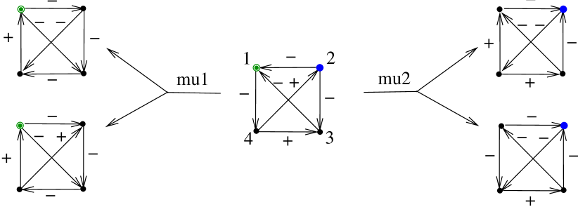
While drawing quivers we will use the following conventions:
-
–
given an arrow of weight , we will label this arrow by ; we will also say that is an arrow marked ;
-
–
arrows of weight will be left unlabeled;
-
–
we draw double arrows instead of arrows of weight .
-
–
-
•
We say that an arrow vanishes if and are not joined in .
-
•
By , we denote a rank cyclic quiver with arrows of weights .
-
•
A rank acyclic quiver with arrows of weights looking in one direction and an arrow of weight in the opposite direction will be denoted by , where some weights may equal .
-
•
Given a quiver , we will denote by the quiver obtained from by reversing all arrows. is also called a quiver opposite to .
Theorem 2.2 ([FeTu1], Theorem 6.11).
Let be a connected rank quiver with real weights. Then is of finite mutation type if and only if it is mutation-equivalent to one of the following quivers:
-
(1)
;
-
(2)
, ;
-
(3)
, , , , .
Corollary 2.3.
Let be a connected mutation-finite rank quiver with real weights. Then
-
(1)
All weights of are of the form with , .
-
(2)
If contains an arrow marked with , , then is mutation-equivalent to .
-
(3)
If contains an edge of weight then is a cyclic quiver which coincides with either or , , .
-
(4)
If , is an acyclic quiver, then
-
-
for some , such that ;
-
-
if in addition at least one of equals with , ,
then .
-
-
-
(5)
If , is a cyclic quiver then
-
-
for some , such that (up to permutation of );
-
-
if in addition at least one of equals to with , ,
then .
-
-
The equalities – in Corollary 2.3 have a geometric interpretation: for every mutation-finite quiver there is a spherical or Euclidean triangle with the corresponding angles (the triangle is acute-angled if is acyclic, and has an obtuse angle otherwise). We also remind that the mutations can be modeled by partial reflections, see [FeTu1].
3. High denominators in ranks and higher
In this section we show that there are no high denominator quivers of rank higher than (Theorem 3.8). To prove the theorem, we start with several technical lemmas (Lemma 3.2-3.7) about rank and quivers.
Definition 3.1.
Given a quiver , we say that is the highest denominator in the mutation class of if all weights of quivers in the mutation class of are either or of the form with , and there exists a quiver in the mutation class of with an arrow of weight , . Abusing notation, we will say that is a denominator quiver.
Lemma 3.2.
No connected mutation-finite quiver contains the Markov quiver as a proper subquiver.
Proof.
Suppose the contrary, i.e. with is a mutation-finite quiver. By Corollary 2.3(3) all rank 3 subquivers of should be cyclic, which is clearly impossible. ∎

Lemma 3.3.
Let be a connected mutation-finite quiver of rank . Suppose that is the highest denominator of weights of arrows in the mutation class of . Then either or is mutation-equivalent to one of the quivers listed in Fig. 3.1.
Proof.
Consider such a quiver . We can assume that has an arrow of weight , , and and are coprime. Let be a rank connected subquiver of containing an arrow of weight . Then corresponds to a Euclidean triangle, and hence, the mutation class of contains an oriented subquiver with weights (without loss of generality we can assume that this is the subquiver itself, and is the double arrow). Moreover, as a mutation-finite rank subquiver with a double arrow cannot be a Markov quiver (see Lemma 3.2), should be a cyclic quiver with the weights ) for some , (see Corollary 2.3(4)). We conclude that is the quiver shown in Fig. 3.2, where the weight of is with , (note that the arrow may be oriented in the opposite way – this would mean the quiver in Fig. 3.2 is the opposite quiver ).

Consider the acyclic subquiver : as it contains an arrow of weight with , Corollary 2.3(4) implies
| (3.1) |
We will consider three cases: either (i.e. the arrows and vanish), or (the arrow vanishes), or otherwise, all six arrows are present in .
Case 1. If , then . Since , we conclude that for some , which implies , , and is the quiver shown in the middle of Fig. 3.1.
Case 2. If , then , so that , and (where ), which produces the quiver on the left of Fig. 3.1.
Remark 3.4.
The following lemma can be verified by a straightforward computation.
Lemma 3.5.
Let where , . Let be an acyclic quiver of rank and be a non-sink/source mutation of . Then
-
(a)
if , then ;
-
(b)
if , then .
Remark 3.6.
The quiver in Lemma 3.5 corresponds to an acute-angled Euclidean triangle with angles , so the statement can also be easily checked by applying partial reflections.
Lemma 3.7.
Let be an acyclic connected rank quiver. Suppose that the vertex is not joined with in . If the weight of is with , , then is mutation-infinite.
Proof.
Suppose that is mutation-finite, and assume first that is neither a sink nor a source. In particular, it is connected to both and . Then, as is acyclic, the mutation at vertex changes the weight of the arrow but does not change its direction.
Now, consider the subquiver . Since the arrow incident to has the weight with , we conclude that the acyclic subquiver can be modeled by an acute-angled Euclidean triangle, and moreover, the weight of the arrow is uniquely determined by the weights of and . Since is not joined with , the mutation preserves the weights and directions of arrows and . Since also preserves the direction of , this implies that the subquiver of the mutated quiver is still acyclic and satisfies the same properties as : it is modeled by an acute-angled Euclidean triangle. Hence, the weight of the new arrow should coincide with the weight of the old arrow . This contradicts the result of the paragraph above. The contradiction shows that is mutation-infinite.
Assume now that is either a sink or a source. We will now show that applying sink/source mutations only we can make neither a sink nor a source, and thus reduce the case to the one already being considered.
Indeed, without loss of generality we can assume is a sink. Applying, if necessary, a source mutation in , we can assume that is not a source. Since is acyclic, it contains a source, and thus either or is a source. After mutating at a source, the vertex is neither a sink nor a source anymore, so we are in the assumptions of the first case.
∎
Theorem 3.8.
There is no rank connected mutation-finite quiver with an arrow of weight with , , .
Proof.
Suppose that is a mutation-finite connected rank quiver, and assume that is a connected subquiver containing an arrow of weight , , . We can assume that is the highest denominator in the mutation class of . Then by Lemma 3.3, is mutation-equivalent to one of the quivers in Fig. 3.1 or its opposite. Without loss of generality we may assume that the subquiver of itself is one of the quivers in Fig. 3.1. We consider these three series of quivers separately.
Case 1: Odd denominator . Then is the subquiver shown in Fig. 3.1 on the right (we can assume is the double arrow and is the vertex incident to two arrows marked ). By reasoning as in Case 3 of the proof of Lemma 3.3, we see that the subquiver looks identical to modulo the direction of the arrow which can point either way (see Fig. 3.3(a) and (b)). Applying Corollary 2.3(4) to acyclic subquiver we see that the arrow should be marked . In the case shown in Fig. 3.3(b) we also see that the arrow is directed from to (as the weights of arrows in the subquiver require this subquiver to be acyclic); in the case shown in Fig. 3.3(a) the vertices and are completely symmetric, so we can also assume is directed from to . Therefore, the quiver is one of the two quivers shown on the left of Fig. 3.3. Applying mutation in vertex , we obtain the quiver shown on the right of Fig. 3.3 (we use Lemma 3.5 to compute the new weights of arrows). However, the subquiver of is an acyclic subquiver with arrow of weight , which is impossible by Corollary 2.3(3).
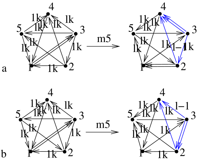
Case 2: Even denominator . In this case there are two possibilities for each of the subquivers and (see Fig. 3.1), which, up to symmetry and taking (and sink/source mutations), gives rise to four forms of the quiver shown in Fig. 3.4. In each of the four possibilities the weight of the arrow is determined uniquely from subquivers or .
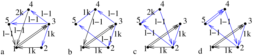
Notice that in cases (a), (b) and (c) the subquiver is acyclic, having a vertex (, and in the three cases respectively) which is not joined with and incident to the arrow of weight , . So, by Lemma 3.7 (and, hence, ) is mutation-infinite.
We are left to consider the case (d). Applying mutations in vertices and the , we obtain the quiver shown in Fig. 3.5. Its subquiver is acyclic, has a denominator arrow , but does not correspond to a Euclidean triangle, so it is mutation-infinite.

∎
4. Low denominator quivers
By low denominator quivers we mean quivers without arrows marked , where , and . There are finitely many of low denominator quivers in each rank, so one can classify mutation-finite low denominator quivers of small ranks checking them case by case.
4.1. Denominator mutation classes
For every skew-symmetrizable integer matrix one can construct a skew-symmetrization of it by putting . Matrix gives rise to a (possibly non-integer) quiver whose mutations agree with mutations of the diagram of (see [FZ2]). Notice that not every non-integer denominator quiver corresponds to a diagram of an integer skew-symmetrizable matrix: to have a corresponding skew-symmetrizable matrix the number of arrows of weight in every (not obligatory oriented) cycle must be even (cf. [K, Exercise 2.1]). However, it is easy to check that any chordless cycle with odd number of arrows of weight is mutation-infinite, and thus we can conclude that the finite mutation classes of denominator quivers are the same as the ones described in [FeSTu2].
Remark 4.1.
Denominator and quivers are actually integer, so we do not need to consider them.
Corollary 4.2.
Any mutation-finite quiver with highest denominator is mutation-equivalent to a symmetrization of one of the integer diagrams, i.e. either it arises from a triangulated orbifold or is one of the exceptional quivers listed in Fig. 4.1 (we call these -type quivers).

4.2. Denominator : separating from
Proposition 4.4.
Let be a quiver of finite mutation type with the highest denominator in the mutation class. Then no quiver in the mutation class of contains a denominator arrow.
Proof.
If some quiver in the mutation class of does not contain arrows with denominators , then the whole mutation class has no such arrows: this is immediate from the mutation rule (as ). Therefore, we can assume that every quiver in the mutation class of contains both denominator and denominator arrows. Without loss of generality we can also assume that is of smallest possible rank with this property. Let be the rank of . In view of classification of mutation-finite rank quivers we see that .
Suppose that is a denominator arrow. By the minimality of , no of the arrows has denominator . This implies that a denominator arrow is contained in . Without loss of generality we can assume that the arrow has denominator .
Consider the shortest path connecting (one of the endpoints of) to (one of the endpoints of) , we can assume that connects to . Since is minimal and is shortest, the support of coincides with and is a linear graph containing all vertices of except for and . Thus, we can assume that the subquiver only contains arrows , and each of these arrows is of weight or . Furthermore, besides the arrows in , denominator arrow and denominator arrow , the quiver may only contain two other arrows: and .
Notice that cannot have denominator as this would contradict the minimality of . Also, cannot have weight or , as in that cases the subquiver would not be mutation-finite. Thus, there is no arrow between vertices and . If has weight then is already mutation-infinite, so we can assume that has weight . Applying (if needed) mutation we can assume that is neither a sink nor a source, so applying mutation we will create a denominator arrow (and this will not affect the rest of the quiver). The subquiver spanned by all vertices but will now contain both denominator and denominator arrows, which contradicts the minimality of .
∎
4.3. Denominator mutation classes
In this section we classify denominator mutation classes (i.e. low denominator quivers containing arrows marked or ). In view of Proposition 4.4, such a quiver only contains arrows marked (such arrows are absent), (simple arrows), , and (double arrows).
The classification can be now achieved by a short (computer assisted) case-by-case study which we organize as follows.
All rank mutation-finite classes are listed in Theorem 2.2 (there are only mutation classes containing arrows of denominator ). The fourth vertex may be added to a representative of each of these mutation classes in ways. Most of the obtained quivers are mutation-infinite, so this will produce mutation-finite classes listed in the left and middle columns of Fig. 4.2. Then one can add the fifth vertex to get two mutation classes of rank . Adding the sixth vertex we get exactly one mutation class, while adding one more vertex to that one does not give any new mutation-finite quivers.
We can now summarize the results of the computation described above.
Theorem 4.5.
A denominator quiver of finite mutation type is mutation-equivalent to one of the quivers listed in Table 4.2.

5. Rank quivers with high denominators
In view of Theorems 3.8 and 4.5 we are left to classify mutation-finite quivers of rank with the largest denominator . By Lemma 3.3 every such quiver is mutation-equivalent to one of the quivers shown in Fig. 3.1. In other words, we are left to study three infinite series of rank quivers. Below, we show that each mutation class in these three families is mutation-finite.
Note that all three series in Fig. 3.1 are infinite (as ), and computing the mutations classes for relatively small one can observe the size of the mutation classes grows with . We will show by induction that all quivers in each of these mutation classes satisfy certain conditions, which will imply mutation-finiteness as the conditions describe a finite set of quivers for every given . The three types of quivers shown in Fig. 3.1 will be treated separately (but in a very similar way).
Lemma 5.1.
The quiver shown on the right of Fig. 3.1 is mutation-finite for every .
Proof.
We will show by induction (on the number of mutations applied) that every quiver in the mutation class can be presented in a standard form shown in Fig. 5.1 with some parameters satisfying the following conditions:
-
(1)
;
-
(2)
;
-
(3)
;
-
(4)
and .
The mutation-finiteness then follows immediately.

Base of induction. Reordering the vertices, one can redraw the quiver shown on the right of Fig. 3.1 as in Fig. 5.2. In this case , and , which clearly satisfies conditions –.

Step of induction. Our aim is now to show that the class of quivers described in Fig. 5.1 with the conditions (1)–(4) is closed under mutations. A priori, we need to check four mutations for that (one mutation in each of the four directions). However, taking into account the symmetry of the conditions above and considering the quivers up to the opposite allows us to reduce the work to checking the two mutations in the two vertices and , see Fig. 5.1. Indeed, taking to and renumbering vertices according to permutation results in the same quiver with the label swapped with (and swapped with ). Now observe that taking the opposite commutes with mutations, and satisfies the conditions (1)–(4) if and only if does. Therefore, checking the mutation in, say, is equivalent to checking the mutation in .
1. Mutation in . We will first check the mutation . Depending on various values of and , the quiver obtained is of one of the two forms shown in Fig. 5.3 (in the figure we first show the mutation and then redraw the same quiver in the standard form). In computing the new weights of arrows we apply parts (4) and (5) of Corollary 2.3 and use the assumption . Notice also that we obtain a weight (and not ) as in view of assumption (4).
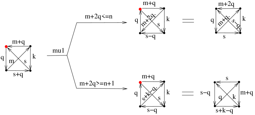
Case 1a: . As follows from Fig. 5.3, the result of this mutation is still a quiver having the standard form shown in Fig. 5.1 with the new values of labels
We now need to check properties (1)–(4) for (using the ones for ). We denote by (1)’, (2)’ etc the corresponding conditions for the mutated quiver.
The properties (1)’–(3)’ for follow immediately from the ones for .
Now, we need to check (4)’. First, (otherwise , so which contradicts the assumption of the Case 1a). Next, we rewrite (4)’ for in terms of the old values:
and prove these four inequalities.
It is clear that and . The inequality also holds as by the assumption of Case 1a. Finally, to prove , assume the contrary, i.e. , and hence . This implies (again, by the assumption of Case 1a), i.e. . However, (1) and (3) imply that or , so we come to a contradiction.
Case 1b: . The new values of the labels are
Now, we verify properties (1)’–(4)’ for :
-
(1)’:
, and hence is equal to either or .
-
(2)’:
We need to check that . The first of these inequalities follows from
while the second one follows from
-
(3)’:
-
(4)’:
First, as in view of the assumption and property (4) for . Next, we check that
as follows:
-
()
As shown in the proof of (2)’, . Thus, .
-
(
If then , which implies in contradiction to (3). Hence, .
-
()
To show consider two cases: and (one of them holds by (1)).
If then and hence (as in view of part () above), which implies .
If then (otherwise, by the assumption of the case 1b, this would imply in contradiction to the assumption ). Therefore, . This means , and thus as required.
-
()
The inequality follows from and .
-
()
2. Mutation in . Now, we need to check the mutation . We follow the same scheme as before: consider two cases as shown in Fig. 5.4 (again, we apply Corollary 2.3 and the assumption that to compute the new weights of some arrows). Notice also that we obtain a weight (rather than ) as otherwise would by (1) imply , and hence which contradicts (4).
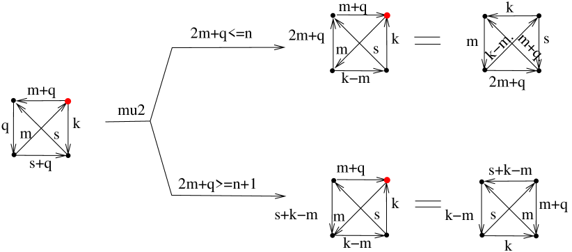
Case 2a: . The new weights of arrows in the standard form are
The conditions (1)’–(4)’ are verified as follows:
-
(1)’
equals either or as it should.
-
(2)’
We need to show .
We start with the latter by noticing that the assumption of Case 2a implies , and hence , i.e. .
Now, (see the proof of (1)’), so we see that (where the second inequality makes use of shown above). If we are done, otherwise, which implies and (as ). Hence, , which by (3) means in contradiction to .
-
(3)’
equals either or by (1).
-
(4)’
The conditions hold as by (4) and as by (1) and by (2)’. Another set of inequalities rewrites as
and can be proved as follows:
-
()
Clearly, .
-
()
By the assumption of Case 2a, , hence, .
-
()
as .
-
()
We need to show which is equivalent to . Suppose the contrary, i.e. , then applying (1) and the assumption of Case 2a we have which is impossible.
-
()
Case 2b: . The new weights of arrows in the standard form are
The computations in this case are a bit more involved than before:
-
(1)’
, hence, it is still equal to either or .
-
(2)’
We need to show .
The first of these inequalities is obtained (using the assumption of Case 2b) as follows:
To prove the second inequality, we apply the assumption of Case 2b again and compute
which gives the required inequality if .
If then by (1) we have . Also, the assumption of Case 2b then reads as . Therefore,
as required.
-
(3)’
as required.
-
(4)’
The inequalities hold as , . The inequalities
can be checked as follows:
-
()
as .
-
()
as otherwise which (together with the assumption of Case 2b) implies which contradicts (1).
-
()
as otherwise , implying ; by (1) and (3) this means , i.e. which is impossible.
-
()
To show assume the contrary, i.e. , then
which implies that in contradiction to (3).
-
()
As no of the two mutations takes the quiver away from the (finite) set of quivers having the standard form described by Fig. 5.1 and conditions (1)–(4), we conclude that the mutation class is finite.
∎
Using very similar computations we prove the following lemma.
Lemma 5.2.
The quivers shown on the left and in the middle of Fig. 3.1 are mutation-finite for every .
To prove this lemma we use exactly the same standard form of the quivers (see Fig. 5.1) together with a marginal variation of the set of conditions (see Table 5.1). These variations (as well as different shapes of quivers) are due to different parity of the denominator: there is one mutation class for every with odd denominator , while in the case of the even denominator the set of quivers splits into two mutation classes for every (see also Proposition 5.3).
![[Uncaptioned image]](/html/1902.01997/assets/x14.png)
Proposition 5.3.
Proof.
From the proof of Lemmas 5.1 and 5.2 we see that applying mutations to any quiver represented in the standard form and satisfying one of the three versions of the conditions we always obtain quivers of the same family. As each family is finite for any given , this shows mutation-finiteness of .
We are left to discuss which quivers belong to the same class. It is clear that quivers with different denominators (or with the same even denominator but different sets of conditions) belong to different mutation classes. On the other hand, by Theorem 3.3 every mutation-finite high denominator quiver is mutation equivalent to one of the quivers in Fig. 3.1. So, quivers with the same invariants (i.e. the same denominator and the same set of conditions) are mutation-equivalent, while quivers with different invariants are not.
∎
This concludes the proof of Theorem A.
6. Geometric realization for finite mutation classes
In this section we will show that every non-integer mutation-finite mutation class (except, possibly, for ones of the orbifold type) admits a geometric realization by reflections in some positive semi-definite quadratic space . This will allow us to define the finite, affine and extended affine types of quivers.
6.1. Definitions and results
Definition 6.1.
Let be an skew-symmetric matrix corresponding to a quiver , and let be a real quadratic space. We say that a tuple of vectors is a geometric realization of if the following conditions hold:
-
(1)
for , for ;
-
(2)
if is a cycle, then the number of pairs such that is even if is acyclic and odd if is cyclic.
A mutation of is defined by partial reflection:
We say that provides a realization by reflections of the mutation class of if the mutations of agree with the mutations of , i.e. if conditions – are satisfied after every sequence of mutations.
We recall that every acyclic integer quiver admits a realization by reflections [S2, ST]. Following [S1], we give the following definition.
Definition 6.2.
A geometric realization of a quiver by vectors is admissible if for every chordless oriented cycle of the number of positive scalar products is odd, while in every chordless non-oriented cycle such a number is even. A geometric realization of a mutation class is admissible if the realization of every quiver is admissible.
We will start by showing that every non-orbifold finite mutation class of non-integer quivers has a representative possessing an admissible geometric realization.
Lemma 6.3.
Every quiver shown in Table 1.1 has an admissible geometric realization.
Proof.
Every quiver listed in Table 1.1 is of one of the following three types:
-
-
either the rank is (and then it is or );
-
-
or it is acyclic;
-
-
or it has a double arrow, and by removing either end of the double arrow we obtain an acyclic quiver (the two acyclic quivers are the same up to one source/sink mutation).
Quiver is mutation-acyclic of rank , and thus has an admissible realization by [FeTu1].
For an acyclic quiver , we define inner product on vectors by , , where is the weight of the arrow . Clearly, is an admissible realization of .
For the last type of quivers, assume that the ends of the double arrow are and . We take the acyclic subquiver obtained by removing , define inner product on vectors for the acyclic subquiver as described above, and then define , for . Then is an admissible realization of . ∎
Remark 6.4.
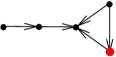
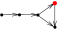
The condition that is not of orbifold type is necessary for Lemma 6.3: it is easy to check that already the surface quiver shown in Fig. 6.1(a) has no admissible geometric realization. This quiver defines a triangulation of a once punctured annulus, another representative of the same mutation class is shown in Fig. 6.1(b).

Theorem 6.5.
Let be a real mutation-finite quiver of rank higher than not originating from an orbifold. Then the mutation class of admits a geometric realization by reflections in a positive or semi-positive quadratic space . In particular, the quadratic form has the kernel of dimension
Proof.
In Lemma 6.3 we have constructed geometric realizations for representatives of required mutation classes, so we only need to show that these geometric realizations can be extended to the whole mutation classes. For rank mutation classes we know the result from [FeTu1]. For the three series in rank this will be done in Section 6.2. Other mutation classes are treated case-by-case.
The case-by-case check is done via a code which verifies that the realization of the initial quiver propagates as a realization of the whole mutation class. The algorithm is the following: we apply a mutation to a quiver and the partial reflections to the corresponding set of vectors (i.e., mutate the Gram matrix according to the rules prescribed in [BGZ]), and then verify that the mutated Gram matrix provides an admissible realization of the mutated quiver. Notice that the mutated Gram matrix only depends on the initial Gram matrix and the directions of arrows in the corresponding quiver before the mutation, but does not depend on the actual vectors . The code checks that in each of the (non-serial) finite mutation classes the pair (Gram matrix; exchange matrix) takes only finitely many values and the entries in the Gram matrix and the exchange matrix agree, i.e. for .
The dimension of the kernel can be easily seen from the initial construction in Lemma 6.3. ∎
Remark 6.6.
It follows from Remark 6.4 that already the mutation class of a quiver originating from a punctured annulus (see Fig. 6.1) does not have an admissible realization by reflections. This implies that most non-acyclic mutation classes of punctured surfaces or orbifolds do not possess admissible realizations by reflections.
Geometric realizations by reflections of all mutation classes of quivers originating from unpuctured surfaces were constructed in [FeLSTu]. There is a strong evidence for the following conjecture.
Conjecture 6.7.
Every mutation class originating from an unpunctured orbifold admits a realization by reflections.
6.2. Geometric realizations for rank series
In rank we have infinitely many finite mutation classes whose sizes are not uniformly bounded, so we are not able to apply a computer verification. We start with proving the following technical lemma.
Lemma 6.8.
Proof.
can have a vanishing arrow in the only case when the highest denominator of is even, and hence is mutation-equivalent to the quiver on the left or in the middle of Fig. 3.1. For each of these quivers (considered in the standard form) we check which arrows can vanish (we use the conditions shown in Table 5.1 for that; an arrow marked vanishes if and only if ). In particular, condition (2) implies that .
Further, if then the conditions imply that no other arrow vanish, and moreover, the quiver is as on Fig. 6.2(a) or (e). If we check the case and get the quiver on Fig. 6.2(b) (there are no such quivers in the other mutations class). The same (up to symmetry) will happen if . Finally, if and we obtain the quivers in Fig. 6.2(c) and (f). If, in addition, we require , we get the quivers shown in Fig. 6.2(d) and (g).
∎

Lemma 6.9.
Let be a quiver in its standard form (see Fig. 5.1) and its admissible geometric realization. Then for every the collections of vectors provide geometric realizations of .
Proof.
The proof is by induction on the number of mutations needed to reach a given quiver from the initial quiver shown in Fig. 3.1. We start with a quiver shown in Fig. 3.1 and consider its admissible geometric realization constructed in Lemma 6.3. Given a quiver in the mutation class and its admissible realization , we will apply all four possible mutations (mutating the set of vectors using partial reflections) and check that the mutated set of vectors provides an admissible geometric realization for the mutated quiver (note that, as in Lemma 5.1, we actually need to check only two mutations, the other two follow from a symmetry of the quiver provided by taking with a permutation of vertices). Since is an admissible realization for , we conclude that is a geometric realization for (see [BGZ, Proposition 3.2]), and we only need to show that is an admissible geometric realization for .
We start checking the admissibility of by considering the case of odd denominator: this will be the easiest case as no quiver in the mutation class has vanishing arrows.
Case 1: odd denominators. We label an arrow of by “” (resp. “”) if is positive (resp. negative).
Applying a mutation we compute the new sign labels as follows. First, we compute the new labels of all arrows incident to : these labels easily follow from the mutation rule (which says that either both vectors are reflected in and, hence, the sign is preserved, or only is substituted by its negative, and then the sign changes to the opposite). The label for an arrow non-incident to is computed from the triangle : namely, the number of arrows labeled by “” in should be even if and only if is cyclic by [FeTu1]. When all labels are computed, we check the rank subquiver and see that the labeling is also admissible on this rank subquiver, see Fig. 6.3. This implies that is an admissible realization for (indeed, in the assumption of odd denominator we only need to check cycles of length ). Notice that as all quivers in the mutation class are ones in the standard form and no arrow vanishes from it, mutations considered in Fig. 6.3 exhaust all possibilities for the case of odd denominator (here, we use the two possible forms of mutated quiver explored in the proof of Lemma 5.1, see Figs. 5.3 and 5.4).
Case 2: even denominators. We follow exactly the same plan as for odd denominator, however, we need to consider the quivers with some vanishing arrows separately (as in this case we need to take additional care while mutating the sign labels).
In Lemma 6.8 we list the quivers with vanishing arrows appearing in the considered mutation classes. Given a quiver from one of the two series, we need to do the following:
-
(1)
if has no vanishing arrows and is an admissible geometric realization of , then we need to check the admissibility of the realization ;
-
(2)
if has vanishing arrows, is an admissible geometric realization of and , then we need to check whether is a geometric realization of , and whether it is admissible.
In the first of these checks the condition for cycles of length is verified by the same computation as before, however, we need to check also cycles of length (as may have vanishing arrows). As we can see from the list in Fig. 6.2, a length chordless cycle is always oriented (for quivers in these mutation classes). As one can check in Fig. 6.3, an oriented cycle of length always receives an odd number of labels “”, even when this cycle is not a chordless one. This verifies the condition for cycles of length , and hence we can assume that has at least one vanishing arrow.
To complete the second check above, we need to mutate the quiver. As before, we label the arrows of with “” and “” in an admissible way (which exists by the induction assumption). Note that for each of the quivers in the list there is a unique way to choose such a labeling (up to changing signs of some of vectors ). We will only need to look at the mutations in the directions of vertices incident to some vanishing arrows (all other mutations are treated in exactly the same way as before). Also, we do not need to check the mutations with respect to sink or source as they do not change signs in any oriented cycle and change exactly two signs in a non-oriented one. Furthermore, we will use symmetries of quivers (and the symmetry up to taking ) to reduce the computations. This reduces the list of cases to the one in Fig. 6.4.
To compute the signs after mutation we do the following. First, we compute the signs of all arrows incident to as before. Then, we compute the signs of all arrows where both and are connected to by a non-vanishing arrow. All the other signs remain intact (indeed, if both and are not joined to then and ; if the arrow vanishes and does not, then , while may either coincide with or computes as , in both cases we have ). The computation shows that is an admissible realization of .
∎

Remark 6.10.
Once we have geometric realization of a mutation class by reflections, we can consider the set of all mirrors of reflections obtained by iterated mutations of the initial tuple of vectors. Then it is easy to see that a quiver is of finite type if and only if the corresponding set of mirrors is finite (and coincides with the hyperplane arrangement associated to a finite Coxeter group).
7. Acyclic quivers and acute-angled simplices
For non-integer quivers of finite or affine type, geometric realization constructed in Lemma 6.3 defines an acute-angled simplex bounded by the mirrors of reflections of the corresponding finite or affine Coxeter group (, , , , or and affine versions of them). It is natural to ask the following two questions:
-
(1)
Given a mutation-finite acyclic quiver, does it always correspond to an acute-angled simplex defined by the geometric realization (up to a change of signs of some of the vectors )?
-
(2)
Given an acute-angled simplex defined by some roots of a root system in , does it give rise to a realization of a mutation-finite quiver?
Notice that in rank the answers to both of these questions are positive, see [FeTu1]. Moreover, for integer quivers this also holds: in finite (respectively, affine) types , , , , , and every acyclic quiver defines an acute-angled spherical (respectively, Euclidean) Coxeter simplex, and any acyclic orientation of a Coxeter diagram of a Coxeter simplex gives rise to a mutation-finite quiver.
We will now see that the situation in the general case is more involved.
7.1. Acute-angled simplices for all acyclic representatives
The answer to the first question is positive also in the general non-integer case. We have checked it case-by-case (but we have no conceptual proof at the moment). In Table 7.1 we list all acyclic quivers (up to sink-source mutations) in the mutation classes containing more than one acyclic representative.
![[Uncaptioned image]](/html/1902.01997/assets/x19.png)
7.2. Not all acute-angled simplices give rise to mutation-finite acyclic quivers
It turns out that the answer to the second question is negative.
By a diagram of a simplex we will mean a counterpart of a Coxeter diagram, i.e. a weighted graph, where vertices correspond to the facets of the simplex, and the weights of the edges denote the dihedral angles (the edges with label are omitted, the edges corresponding to are unlabeled). We have written out the complete list of diagrams of acute-angled simplices in root systems , and and checked that most of these simplices appear as geometric realizations of some mutation-finite acyclic mutation classes. However, there is a number of exceptions: in Table 7.2 we list all (up to sink/source mutations) mutation-infinite acyclic quivers appearing as orientations of diagrams of acute-angled simplices in , and .
It is currently not clear to us what distinguishes the acute-angled simplices appearing in Tables 7.2 from ones defining mutation-finite quivers, and we think it would be an interesting question to understand the source of this difference.
![[Uncaptioned image]](/html/1902.01997/assets/x20.png)
Remark 7.1.
Finally, we list some observations concerning the acute-angled simplices and the corresponding quivers.
-
(a)
Every acute-angled simplex in , , or either is decomposable (i.e., its diagram is disconnected), or is a spherical Coxeter simplex of the type or , or has a diagram whose orientation appears either in Table 7.1 or in Table 7.2 (or in both: two distinct acyclic orientations of the same simplex diagram may not be simultaneously mutation finite/infinite).
-
(b)
Notice that when a diagram of a simplex has a cycle of length more than , there are two acyclic orientations of such a diagram up to sink/source mutations. All other diagrams arising from acute-angled simplices have a unique acyclic orientation up to sink/source mutations.
- (c)
-
(f)
Acute-angled simplices in finite types are also listed in [Fe].
-
(g)
The affine extensions of Coxeter groups of type were described in [PT]. In particular, the diagram of the simplex giving rise to the top left quiver in Table 7.2 was used to define the group . We note that one can start with any of the simplices whose diagrams are listed in the parts of Tables 7.1 and 7.2 to get the same group.

References
- [BBH] A. Beineke, T. Brüstle, L. Hille, Cluster-cyclic quivers with three vertices and the Markov equation, With an appendix by Otto Kerner, Algebr. Represent. Theory, 14 (2011), 97–112.
- [BGZ] M. Barot, C. Geiss, A. Zelevinsky, Cluster algebras of finite type and positive symmetrizable matrices, J. London Math. Soc. (2) 73 (2006), 545–564.
- [DT] D. Duffield, P. Tumarkin, Categorifications of non-integer quivers: types , and , arXiv:2204.12752
- [Fe] A. Felikson, Spherical simplices generating discrete reflection groups, Sb. Math. 195 (2004), 585–598.
- [FeLSTu] A. Felikson, J. W. Lawson, M. Shapiro, P. Tumarkin, Cluster algebras from surfaces and extended affine Weyl groups, Transform. Groups 26 (2021), 501–535.
- [FeSTu1] A. Felikson, M. Shapiro, P. Tumarkin, Skew-symmetric cluster algebras of finite mutation type, J. Eur. Math. Soc. 14 (2012), 1135–1180.
- [FeSTu2] A. Felikson, M. Shapiro, P. Tumarkin, Cluster algebras of finite mutation type via unfoldings, Int. Math. Res. Notices 8 (2012), 1768–1804.
- [FeSTu3] A. Felikson, M. Shapiro, P. Tumarkin, Cluster algebras and triangulated orbifolds, Adv. Math. 231 (2012), 2953–3002.
- [FeTu1] A. Felikson, P. Tumarkin, Geometry of mutation classes of rank quivers, Arnold Math. J. 5 (2019), 37–55.
- [FeTu2] A. Felikson, P. Tumarkin, Acyclic cluster algebras, reflection groups, and curves on a punctured disc, Adv. Math. 340 (2018), 855–882.
- [FG] V. Fock, A. Goncharov, Dual Teichmüller and lamination spaces, in: Handbook on Teichmüller theory, vol. 1, 647–684, Europ. Math. Soc., 2007.
- [FST] S. Fomin, M. Shapiro, D. Thurston, Cluster algebras and triangulated surfaces. Part I: Cluster complexes, Acta Math. 201 (2008), 83–146.
- [FT] S. Fomin, D. Thurston, Cluster algebras and triangulated surfaces. Part II: Lambda lengths, Mem. Amer. Math. Soc. 255 (2018), no. 1223, v+97.
- [FZ1] S. Fomin, A. Zelevinsky, Cluster algebras I: Foundations, J. Amer. Math. Soc. 15 (2002), 497–529.
- [FZ2] S. Fomin, A. Zelevinsky, Cluster algebras II: Finite type classification, Invent. Math. 154 (2003), 63–121.
- [GSV] M. Gekhtman, M. Shapiro, A. Vainshtein, Cluster algebras and Weil-Petersson forms, Duke Math. J. 127 (2005), 291–311.
- [K] V. Kac, Infinite-dimensional Lie algebras, Cambridge Univ. Press, London, 1985.
- [L] P. Lampe, On the approximate periodicity of sequences attached to non-crystallographic root systems, Exp. Math. 27 (2018), 265–271.
- [PT] J. Patera, R. Twarock, Affine extension of noncrystallographic Coxeter groups and quasicrystals, J. Phys. A: Math. Gen. 35 (2002), 1551–1574.
- [R] N. Reading, Universal geometric cluster algebras, Math. Z. 277 (2014), 499–547.
- [S1] A. Seven, Cluster algebras and semipositive symmetrizable matrices, Trans. Amer. Math. Soc. 363 (2011), 2733–2762.
- [S2] A. Seven, Cluster algebras and symmetric matrices, Proc. Amer. Math. Soc. 143 (2015), 469–478.
- [ST] D. Speyer, H. Thomas, Acyclic cluster algebras revisited, Algebras, quivers and representations, Abel Symp., vol. 8, Springer, Heidelberg, 2013, pp. 275–298.