Are All Layers Created Equal?
Abstract
Understanding deep neural networks is a major research objective with notable experimental and theoretical attention in recent years. The practical success of excessively large networks underscores the need for better theoretical analyses and justifications. In this paper we focus on layer-wise functional structure and behavior in overparameterized deep models. To do so, we study empirically the layers’ robustness to post-training re-initialization and re-randomization of the parameters. We provide experimental results which give evidence for the heterogeneity of layers. Morally, layers of large deep neural networks can be categorized as either “robust” or “critical”. Resetting the robust layers to their initial values does not result in adverse decline in performance. In many cases, robust layers hardly change throughout training. In contrast, re-initializing critical layers vastly degrades the performance of the network with test error essentially dropping to random guesses. Our study provides further evidence that mere parameter counting or norm calculations are too coarse in studying generalization of deep models, and “flatness” and robustness analysis of trained models need to be examined while taking into account the respective network architectures.
Keywords: Deep Learning, Overparameterization, Robustness, Generalization, Understanding
1 Introduction
Deep neural networks have been remarkably successful in many real world machine learning applications. The practical success of excessively large networks cannot be explained by the classical wisdom of uniform convergence and learnability. In many critical applications, such as self-driving vehicles and automatic medical diagnostics, distilled understanding of the systems can be as important as achieving the state-of-the-art performance. One important question is on interpreting and explaining the decision function of trained networks. It is closely related to another important topic on networks’ generalization and robustness under drifting or even adversarially perturbed data distribution. In this paper, we study how individual layers coordinate the computation in trained neural network models, and relate the empirical results to generalization and robustness properties.
Theoretical research of the functions computed by neural networks dates back to the ’80s. It is known that a neural network with a single (sufficiently wide) hidden layer is a universal approximator for continuous functions over compact domains (Cybenko, 1989; Hornik et al., 1989; Hornik, 1991; Devroye et al., 2013; Györfi et al., 2006; Anthony and Bartlett, 2009). More recent research further examines whether deep networks can have superior representation power than shallow ones with the same number of units or edges (Pinkus, 1999; Delalleau and Bengio, 2011; Montufar et al., 2014; Telgarsky, 2016; Shaham et al., 2015; Eldan and Shamir, 2015; Mhaskar and Poggio, 2016; Rolnick and Tegmark, 2017). The capacity to represent arbitrary functions on finite samples is also extensively discussed (Hardt and Ma, 2017; Zhang et al., 2017; Nguyen and Hein, 2018; Yun et al., 2018). However, the constructions used in the aforementioned work for building networks approximating particular functions are typically “artificial” and are unlikely to be obtained by gradient-based learning algorithms. We focus instead on empirically studying, post-training, the role different layers take in representing a learned function by gradient-based methods.
Generalization is a fundamental theoretical question in machine learning. The recent observation that big neural networks can fit random labels on the training set (Zhang et al., 2017) makes it difficult to apply classical learning theoretic results based on uniform convergence over the hypothesis space. One approach to get around this issue is to show that, while the space of neural networks of a given architecture is huge, gradient-based learning on “well behaved” tasks leads to relatively “simple” models. More recent research focuses on the analysis of the post-training complexity metrics such as norm, margin, robustness, or flatness of the learned model in contrast to the pre-training capacity of the entire hypothesis space. This line of work obtained sharper generalization bounds for for neural networks (e.g. Kawaguchi et al., 2017; Bartlett et al., 2017; Neyshabur et al., 2017; Liang et al., 2017). In another line of work, Belkin et al. show that overparameterization and perfectly fitting the training set (i.e. interpolation) is not an issue for generalization (e.g. Belkin et al., 2018a, b, c; Azizan et al., 2019). Further more, they argue that even norm-based generalization bounds could become non-informative in the regime of interpolation. Our work provides further empirical evidence and alludes to more fine-grained analysis. We propose that the layers in a deep network are not homogeneous in the role they play at representing a predictor. Some layers are critical to forming good predictions while others are robust as they are fairly insensitive to the assignment of their weights during training. Thus, depending on the capacity of the network and the complexity of the target function, gradient-based trained networks conserve the complexity by not using excess capacity.
Before proceeding, we would like to further mention a few related papers. Modern neural networks are typically overparameterized and thus redundant in their representations. Previous work exploited overparameterization to compress (Han et al., 2015) or distill (Hinton et al., 2015) a trained network. It is also shown that one can achieve comparable performance by training only a small fraction of network parameters such as a subset of the channels in each convolutional layer (Rosenfeld and Tsotsos, 2018). As a tool for interpreting residual networks as ensemble of shallow networks, Veit et al. (2016) found that residual blocks in a trained network can be deleted or permuted to some extent without degrading the test performance too much. Another line of research showed that under extreme overparameterization, such as when the network width is polynomial in the training set size and input dimension (Allen-Zhu et al., 2018; Du et al., 2018a, b; Zou et al., 2018), or even in the asymptotic regime of infinite width (Jacot et al., 2018; Lee et al., 2019), the network weights move slowly during training. We make similar observations in this paper. However, we find that in more pragmatic settings (network widths in the order of thousands), different layers exhibit different behaviors and the network cannot be treated in a monolithic way.
Notice that our work, as well as the literature cited above, focuses on conventional neural networks, where the output of the optimization process is a single set of parameters computing a deterministic function. There is an important, though less related, line of work that considers stochastic neural networks where the output of the training process is a distribution over model parameters. Under this setting, generalization bounds are derived with PAC-Bayes analysis (e.g. Neyshabur et al., 2018; Arora et al., 2018; Zhou et al., 2019; Rivasplata et al., 2019), and in some cases bounds with non-vacuous values can be computed numerically (e.g. Dziugaite and Roy, 2017; Rivasplata et al., 2019). As will be shown in Section 6, the layer robustness properties identified in this paper can be used to turn a deterministic model trained with the conventional methods into a stochastic model.
The rest of the paper is organized as follows. Our experimental framework and notions of robustness to modifications of layers are introduced in Section 2. Section 3 presents the results and analysis of layer robustness for a wide range of neural network models. Section 4 presents experiments with joint robustness. Section 5 shows the generalizability of the phenomenon in alternative domains and architectures. In Section 6 we discuss connections to other notions of robustness. Finally, the paper ends on Section 7 with a discussion and summarization of our main contributions.
2 Setting
We focus on feed forward networks which consist of multiple layers where each unit in a layer takes inputs from units in the previous layer. Let be the function space of a (particular) neural network architecture with (parametric) layers. Each admissible is a list with from for all . We are interested in analyzing post-training characteristics of layers used in popular deep networks. Such networks are typically trained using stochastic gradient descent (SGD) which initialize the parameters by sampling from a pre-defined distribution over . The choice of typically depends on structural properties such as fan-in, and fan-out of each layer. In our experiments, we take the default initialization schemes used in open source deep learning libraries. After training for epochs, the parameters of the last epoch are used as the final trained model.
In a classification neural network, the decision function maps an input to a class from a finite set of labels. Performance of the trained networks is measured in terms of the agreement between its predicted labels and the true labels on a newly observed test set. Unless noted otherwise, we use the term performance to designate the 0-1 classification accuracy. Our study of the layer structure evaluates the performance along the trajectory throughout the entire sequence of training epochs .
Checkpointing.
We save the model parameters at the end of every epoch during training and call the saved models checkpoints. Checkpoint- consists of the parameters for the final model. There is also a special checkpoint- containing random weights initialized before the training starts.
A deep network constructs a representation of its inputs by incrementally applying transformations defined by each layer. Each layer consists of a linear transformation on its inputs, matrix multiplication, followed by nonlinear activation functions applied to the result of the matrix multiplication. Notable examples are the sigmoid and the Rectified Linear Unit (ReLU) activations. As a result, the representation at a particular layer recursively depends on all the layers beneath. This complex dependency makes it challenging to isolate and inspect each layer independently in theoretical studies. In this paper, we introduce and use the following two empirical probes to inspect the individual layers in a trained neural network.
Re-initialization.
After training concludes, for each layer separately, we re-initialize its parameters by assigning while keeping the rest of the parameters intact. We thus obtain different models where each model is of the form . The models are then evaluated on the test set. The relation of a layer to the effect on performance of re-initializing it is referred to as the re-initialization robustness of the layer. Here denotes the randomly initialized values loaded from checkpoint-. More generally, for each epoch , we can re-initialize the ’th layer to its value on epoch through the assignment , and study the re-initialization robustness of layer w.r.t checkpoint-.
Re-randomization.
As one step further, re-randomization of a layer refers to assigning random parameters by re-sampling using the same distribution used for the initialization of , namely , and evaluating . Analogously, re-randomization robustness of a layer is the relation of that layer to the effect on performance of re-randomizing it.
We emphasize that no re-training or fine-tuning is performed after a network is re-initialized/re-randomized. When a network exhibits negligible111We do not quantify how much “negligible” is, as we believe there is no universal threshold across all models and tasks. Our empirical results indicates that there is no or little ambiguity in categorizing layers due to the sharp difference in performance of robust and critical layers. decrease in performance after re-initializing or re-randomizing of a layer, we say that the layer is robust and otherwise the layer is called critical.
3 Robustness of Individual Layers
The datasets we use in our robustness study are standard image classification benchmarks: MNIST, CIFAR-10, and ImageNet. All networks were trained using SGD with momentum using a piecewise constant learning rate schedule. See Appendix A for further details.
3.1 Fully Connected Networks

We start by examining the robustness of fully-connected networks (FCNs). A FCN consists of fully connected layers each of output dimension followed by a ReLU activation function. The additional final layer is a linear multiclass predictor with one output per class.
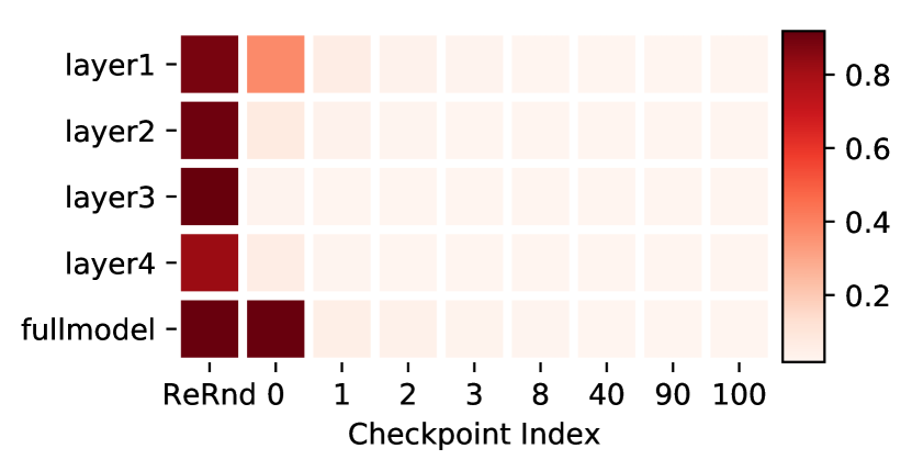
We train an FCN on MNIST and apply the re-initialization and re-randomization analysis on the trained model. The results are shown in Fig. 1(a). As expected, due to the intricate dependency of the classification function on each of the layers, re-randomizing any of the layers completely disintegrates the representation and classification accuracy drops to the level of random guessing. For re-initialization, however, while the first layer is very sensitive the rest of the layers are robust to re-initialization.
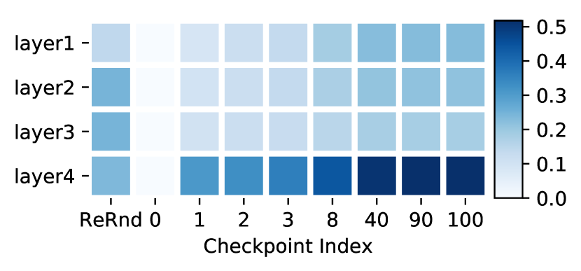
A plausible explanation for this could be attributed to that the increase in gradient norms during back-propagation such that the bottom layers are being updated more aggressively than the top ones. However, if this were the case, we would expect a smoother transition instead of a sharp one at the first layer. Furthermore, we measured how distant the weights of each layer are from their initialization (“checkpoint-0”) using both the -norm (divided by square root of the dimension) and the -norm. The results are shown in Fig. 1 parts (b) and (c), respectively. We can see that robustness to re-initialization is not plainly correlated with either of the distances. This suggests that there might be something more intricate going on than simple gradient expansion. We informally summarize the observations as follows,
Over-capacitated deep networks trained with stochastic gradient descent have low-complexity by a self-restriction of the number of critical layers.
Intuitively, if a subset of parameters can be re-initialized to the random values at checkpoint- (which are independent of the training data), then the the complexity of the model can be reduced. See the discussions in Section 7 for more details.
We apply the same analysis framework to a large number of different FCN architectures to assess the influence of the network capacity and the task complexity on the layer robustness. In Fig. 2(a), we compare the average re-initialization robustness for all layers but the first with respect to FCNs and of varying hidden dimensions () on MNIST. It is clear that the top layers become more robust as the hidden dimension increases. We believe that it reflects the fact that wider FCNs have higher capacity. When the capacity is small, all layers are vigil participants in representing the prediction function. As the capacity increases, it suffices to use the bottom layer while the rest act as random projections with non-linearities.
Similarly, Fig. 2(b) shows experiments on CIFAR-10, which has the same number of classes and comparable number of training examples as MNIST yet it poses a more difficult learning task. Similar traits are observed as the hidden dimensions increase, though not as pronounced as in MNIST. Informally put, the difficulty of the learning task seems to necessitate more diligence of the layers in forming accurate predictors.
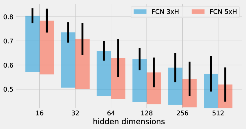
The empirical results of this section provide some evidence that deep networks trained with SGD automatically adjust their capacity. When a large network is trained on an easy task, only a few layers seem to be playing a critical role.
3.2 Large Convolutional Networks



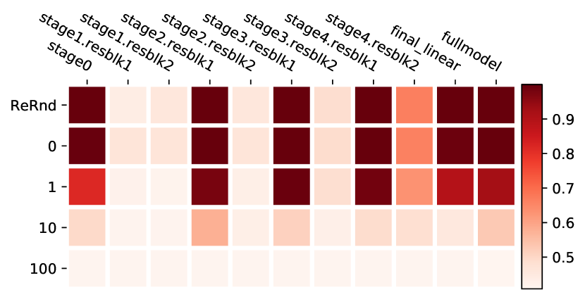
In typical computer vision tasks beyond elementary problems such as MNIST, densely connected FCNs are significantly outperformed by convolutional neural networks. VGGs (Simonyan and Zisserman, 2014) and ResNets (He et al., 2016a, b) are two widely used convolutional network architectures. Fig. 3 and Fig. 4 show the robustness results on CIFAR-10 with the two architectures. Since the networks are much deeper than the FCNs of the previous section, we transpose the heatmaps and now a column designates a layer. For VGGs, more layers are sensitive to re-initialization, yet the characteristics are similar to the observations from the simple FCNs on MNIST: bottom layers are evidently more sensitive than the top layers to re-initialization.
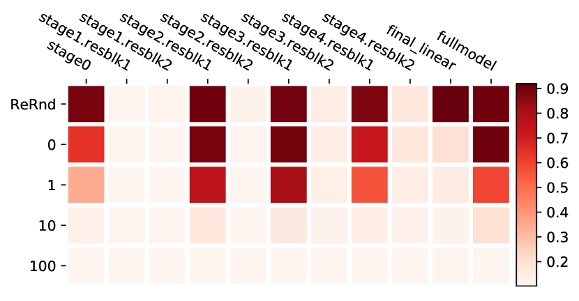


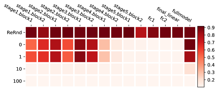
The results for ResNets in Fig. 4 are to be considered together with results on ImageNet in Fig. 5. We found the robustness structure for ResNets to be more interesting for the reasons below.
ResNets re-distribute critical layers.
Unlike FCN and VGG networks for which the critical layers are at the bottom of the network, ResNets sprinkles critical layers throughout the entire depth. To better understand the patterns, let us briefly recap ResNet’s architecture. In practice, a ResNet is divided into “stages”. At the bottom, there is a pre-processing stage (stage0) with vanilla convolutional layers. It is followed by a few (typically 4) residual stages consisting of multiple residual blocks, and lastly a global average pooling operator followed by a linear classifier (final_linear). The image size halves and the number of convolution channels doubles from each residual stage to the next.222There are more subtle details which we omit, especially at stage1 that depend on the input size, whether residual blocks contain a bottleneck, etc.. As a result, while most of the residual blocks have identity skip connections, the first block of each stage (stage*.resblk1), which is connected to the last block of the previous stage, has a non-identity skip connection due to different input-output shapes. Fig. 10 in the Appendix illustrates the two types of residual blocks. In our robustness analysis, we can interpret each stage of a ResNet as a sub-network, with characteristics of layer robustness within each stage similar to VGGs or FCNs.
Residual blocks show robustness to re-randomization.
Among the layers that are robust to re-initialization, if the layer is a residual block, it is also robust to re-randomization, which stands in contrast to the final_linear layer. This could be potentially attributed to that the responses for identity skip connections attain larger values than those of the residual branches. Thus, when summed together residual branches played a less significant role. It is known from prior research (Veit et al., 2016) that residual blocks in a ResNet can be removed without substantially hurting accuracy. Our experiments have a different focus as we study robustness in the light of the interplay between model capacity and the difficulty of the learning task. In particular, comparing the results on the two different datasets, especially on smaller ResNets (e.g. ResNet-18), many residual blocks with real identity skip connection also become sensitive in the more difficult ImageNet task.


4 Joint Robustness
Empirical results we presented thus far focus on individual layer robustness. We next explore joint robustness of multiple layers through simultaneous re-initialization or re-randomization.


We divide the layers into two groups and perform robustness experiments with each group. For ResNets, we put all but the first residual blocks of all stages into one group and jointly re-initialize or re-randomize all the layers in the group. Fig. 6(a) demonstrates that even though each of these layers are all individually robust, as a group they are not jointly robust. However, a different grouping scheme shown in Fig. 6(b) demonstrates that robustness can be significantly improved when jointly resetting about half of the layers for this ResNet architecture. See Appendix B for more details.
Note that SGD fits the model with the aforementioned jointly robust structure without explicit constraints. We next examine if explicit constraints could improve joint robustness. Concretely, we experiment with two approaches: (i) We freeze layers at their random initialization and refrain from training all frozen layers; (ii) We remove layers from the network. Both operations are applied to the groups described above excluding again the first residual block of each stage.
| Arch | Full Model | Individual Layer Robustness | Layers Frozen | Layers Removed | |
|---|---|---|---|---|---|
| (Average) | (Jointly) | (Jointly) | |||
| CIFAR-10 | ResNet50 | 8.40 | 9.771.38 | 11.74 | 9.23 |
| ResNet101 | 8.53 | 8.870.50 | 9.21 | 9.23 | |
| ResNet152 | 8.54 | 8.740.39 | 9.17 | 9.23 | |
| ImageNet | ResNet50 | 34.74 | 38.545.36 | 44.36 | 41.50 |
| ResNet101 | 32.78 | 33.842.10 | 36.03 | 41.50 | |
| ResNet152 | 31.74 | 32.421.55 | 35.75 | 41.50 |
The results are given in Table 1. When we freeze layers, the resulting error is higher than that of the average individual layer robustness measured in a normally trained model. However, the gap is much smaller than when directly assessing the joint robustness. Moreover, on CIFAR-10, we find that similar performance can be achieved even if we entirely remove those layers from the network. In contrast, for ImageNet layer removal results in a significant drop in performance. In this case, random projections followed by non-linear activations conducted by frozen layers deem necessary to maintain accuracy.
5 Other Architectures and Domains
In this section, we study the generalizability of the layer robustness phenomenon by extending the evaluation to a different domain (language modeling) and different model families (convolution-free architectures). We find the results corroborate the key observations made earlier in this paper.
5.1 Transformer Based Neural Language Models
We consider a 12-layer decoder-only (Liu et al., 2018) Transformer (Vaswani et al., 2017) based neural language model, more specifically, the decoder-only version of the T5-Base (Raffel et al., 2020) model. It has 112,242,480 parameters. We train it on the LM1B (Chelba et al., 2013) dataset, which is a popular benchmark corpus for language modeling with 30,301,028 training examples (around one billion words). We use the SentencePiece333https://github.com/google/sentencepiece. tokenizer with a vocabulary size of 30,000. We train the model with Adam optimizer (Kingma and Ba, 2015) for 20 epochs.
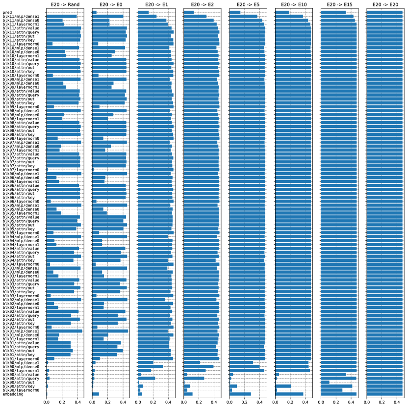
We then measure the robustness of this model on the validation set with the average per-token accuracy. Figure 7 show the results for re-randomization, and re-initialization to epoch 0, 1, 2, 5, 10, 15 and 20, respectively. The results for re-randomization and re-initialization to epoch-0 look very similar, except for the embedding and the pred layers. Note the pred layer performs a 30,000 way classification to predict the next token. This is consistent with our earlier observation comparing CIFAR-10 and ImageNet that the final prediction layer is only robust when the number of classes is small. In a language model, the embedding layer maps each of the 30,000 input tokens to a dense embedding vector, and in some architectures it simply shares weights with the pred layer.
The overall trend that higher layers are more robust than lower layers still holds. But we also see some patterns unique to the transformer architecture. For example, the layer normalization (Ba et al., 2016) layers are generally not robust. The first dense layer in each of the MLP block is also sensitive to re-initialization or re-randomization. On the other hand, the second dense layer in each MLP block, as well as all the components in the attention blocks are generally robust (except for block00/*).
Another interesting difference comparing to the vision experiments is that many of the unrobust layers become robust after only one epoch of training. This is likely due the much larger training set sizes in the text domain.

5.2 Convolution-Free Architectures for Computer Vision
In this section, we provide preliminary studies for two new neural network architectures in computer vision that achieve the state-of-the-art performance in image classification benchmarks without using convolution layers. In particular, we consider the attention (Vaswani et al., 2017) based Vision Transformers (ViTs, Dosovitskiy et al., 2021) and the MLP based MLP-Mixers (Tolstikhin et al., 2021). We use the publicly released pre-trained checkpoints444https://github.com/google-research/vision_transformer. that are trained for ImageNet. Since two variants of ImageNet datasets (Deng et al., 2009) were used when training those models, in this subsection, we will spell out the variants as ImageNet-21k — the larger dataset containing 21,000 classes and 14M training images, and ImageNet-1k — the smaller dataset containing 1,000 classes and 1.2M training images. In particular, ImageNet-1k is the same as the “standard” ImageNet dataset used in the rest of this paper.
We run robustness evaluation on the ImageNet-1k validation set. We use checkpoints that can be directly evaluated on ImageNet-1k. In particular, for ViTs, we have access to checkpoints that are pre-trained on ImageNet-21k and then finetuned on ImageNet-1k. We evaluate two variants: ViT-B/16 (86,567,656 parameters) and ViT-L/16 (304,326,632 parameters). For MLP-Mixers, we have access to checkpoints that are directly trained on ImageNet-1k. We also evaluate two variants: Mixer-B/16 (59,880,472 parameters) and Mixer-L/16 (208,196,168 parameters). Additionally, several new checkpoints trained with the Sharpness-Aware Minimization (SAM, Foret et al., 2021) became available recently. We include ViT-B/16-sam, ViT-L/16-sam and Mixer-B/16- in the comparisons (Mixer-L/16-sam checkpoint is not available). All the SAM optimized models are directly trained on ImageNet-1k. Since we do not have access to the original training pipeline and earlier checkpoints, we only perform re-randomization tests on those models.
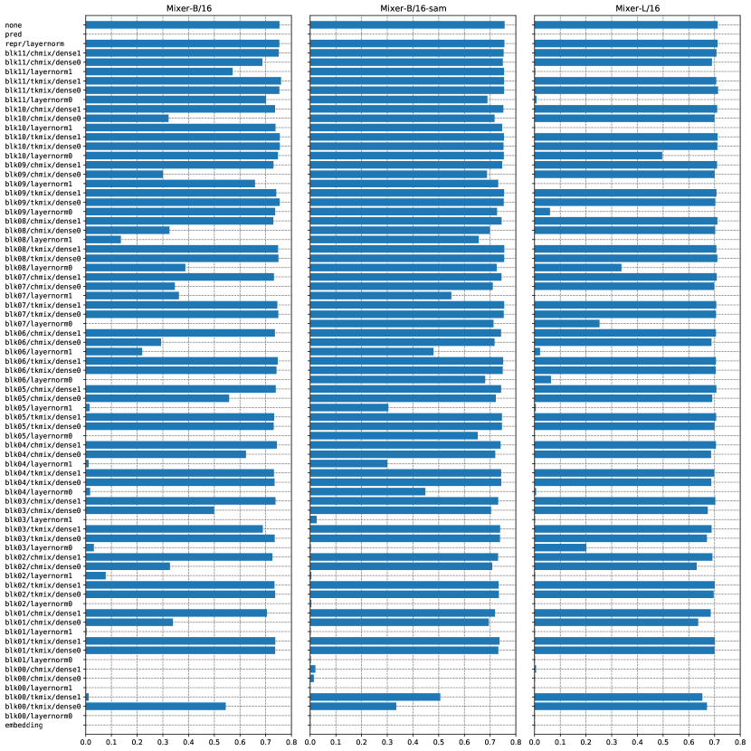
Figure 8 shows the results for ViTs. The ViT architectures are based on the Transformer models for text processing, and we observe the layer robustness patterns are similar to the results on Transformer based language models in Figure 7: the attention related layers and the second dense layer of MLP blocks (mlp/dense1) are generally robust, especially for higher up blocks. We do find more layers (e.g. mlp/dense0) robust here. Comparing among the variants, we find that the larger ViT-L/16 model is generally more robust than the smaller ViT-B/16 model for most layers, except for some layernorm layers the reverse is true. This makes the gap between the robust and non-robust layers more pronounced in the larger model. Comparing each ViT variant with its SAM-optimized version, we see that the SAM optimizer generally improves the robustness for ViT-B/16, and for ViT-L/16 it has an additional effect of making some higher-up layernorm layers even less robust, further enlarging the gap. Figure 9 shows the results for MLP-Mixers. The overall patterns are similar to that of the ViTs.
6 Connections to Other Notions of Robustness
Layer robustness to re-initialization and re-randomization can be related to other notions of robustness in deep learning. For example, flatness refers to robustness to local perturbations of the network’s parameters close to a converged model, and is extensively discussed in the context of generalization (Hochreiter and Schmidhuber, 1997; Chaudhari et al., 2017; Keskar et al., 2017; Smith and Le, 2018; Poggio et al., 2018). For a fixed layer, our notion of robustness to re-initialization is restricted to the training trajectory, which could potentially take the form of a non-local perturbation. Robustness to re-randomization allows for larger variances of perturbations of the trained parameters. As our study shows, robustness seems to be layer-dependent, thus analyzing layers individually for specific network architectures enables us to obtain more refined insights into robustness.
In contrast, adversarial robustness (Szegedy et al., 2013) focuses on robustness to perturbations of the input. In particular, it was found that deep networks are sensitive to small adversarial perturbations which yield prediction shifts to arbitrary classes. A large number of defense and attack algorithms have been proposed in recent years. Here we briefly discuss the connection to adversarial robustness. Take a standard ResNet with stages of residual blocks in each stage. At test time, we turn it into a randomized classifier by selecting at random a subset of stages, and replacing at random a residual block from each of the selected stages with one of the pre-initialized weights of its layer. We keep pre-allocated weights for each residual block instead of re-sampling at random on each evaluation call, primarily to reduce computation during the testing.
From the robustness analysis of previous sections, we expect randomized classifiers to exhibit only a small drop in average performance. However, at the individual example level, randomization of the network’s outputs would make it harder for an attacker to generate adversarial examples. We evaluate the adversarial robustness against a weak FGSM (Goodfellow et al., 2014) attack and a strong PGD (Madry et al., 2017) attack. The results in Table 2 show that compared to the baseline (identical model without output randomization), output randomization significantly improves robustness to weak FGSM attacks. The performances under strong PGD attack drops sharply yet it is still an order of magnitude better than the baseline. The results relate layer robustness to adversarial robustness, but it does not imply randomization via robust layers provides strong adversarial robustness, especially under attacks that are specifically designed with such randomization in mind (Athalye et al., 2018).
To recap, layer robustness can guard a trained model from attack by injecting randomization. However, robustness per se does not provide sufficient defense against strong attacks. More sophisticated attacks that explicitly deal with non-deterministic classifiers could completely render the approach unusable.
| Model Configuration | Clean | FGSM | PGD | |
|---|---|---|---|---|
| baseline | ||||
| r=4,s=1 | ||||
| r=4,s=2 | ||||
| baseline | ||||
| r=4,s=1 | ||||
| r=4,s=2 | ||||
| r=4,s=4 | ||||
7 Discussion
Excessive overparameterization of modern neural network architectures renders conventional generalization bounds based on capacity estimation of the entire hypothesis space unusable. Alternative approaches try to identify nice properties such as bounds on the parameter norms of the models trained with specific algorithms (e.g. SGD) on well behaved data, and derive tighter generalization bounds based on those properties. Our experiments provide useful evidence for deriving tighter generalization bounds via fine grained analysis of layer behaviors.
For example, Chatterji et al. (2020) formulated a notion of module criticality based on our observation of the dichotomy between critical and robust neural network layers, and derived PAC-Bayes generalization bounds. We briefly present their theoretical results below.
Definition 1 (Module and Network Criticality (Chatterji et al., 2020))
Given an and network , we define the module criticality for module as follows:
| (1) |
We also define the network criticality as the sum of the module criticality over modules of the network:
| (2) |
Here denotes the zero-one training loss. indicate the randomly initialized and final trained value of the weight matrix of module . is a convex combination of the two. is the final trained neural network where the weight of its -th module is replaced with . Intuitively, a robust layer could satisfy the condition in (1) with near-zero , therefore has a low criticality value.
Theorem 2 (Chatterji et al. (2020))
For any data distribution , number of samples , for any , for any and any , with probability over the choice of the training set the following generalization bound holds:
| (3) |
where is the number of parameters in module . indicate the network with the weights of each module replaced with , where .
This PAC-Bayes bound characterize perturbed networks. Corollaries that characterize the original network and that provides deterministic generalization can be found in Corollary 3.3 and Appendix B of Chatterji et al. (2020). The existence of robust layers controls complexity terms in the bounds, providing alternative explanation of the generalization power of large overparameterized neural networks. It is shown that this provides more faithful ranking of the generalization power of neural networks than many previous complexity measures (Chatterji et al., 2020, Section 4).
To recap the paper, we empirically investigated the functional structure on a layer-by-layer basis of overparameterized deep models for a wide variety of models for image classification. We introduced the notions of re-initialization and re-randomization robustness. Using these notions we provided evidence for the heterogeneous nature of layers, which can be categorized into either robust or critical. Resetting the robust layers to their initial value has negligible effect on the model’s performance. Our empirical results give further evidence that mere parameter counting or norm accounting is too coarse in studying generalization of deep models. Moreover, optimization landscape based analysis is better performed respecting the network architectures due to the heterogeneous nature of different layers. Our empirical work gives rise to several theoretical questions. We conclude with a short list which is by no means comprehensive of potential directions for future research motivated by our results.
- Lyapunov Function for Deep Architectures.
-
Bregman divergences over the entire set of parameters constitute the tool of choice in analyzing convergence and regret bounds for convex and quasi-convex models. Our results indicate that parameters of a network do not form a monolithic set. Devising novel composite divergences for measuring the progression of learning process is thus deemed useful.
- Formation of robust and critical Layers.
-
As shown, some layers of a deep networks become robust to reset while other layers deem to be critical. This structural symmetry breaking could also shed light on the role of initialization for deep learning.
- Hybrid Algorithms.
-
Our study underscores the potential of hybrid networks of mixed learned and random parameters. Random feature maps for deep learning were studied for fully random representations (Rahimi and Recht, 2008, 2009; Daniely et al., 2016). A potentially high impact direction is devising learning algorithms for building hybrid learned-random networks.
Acknowledgments
We would like to thank David Grangier, Lechao Xiao, Kunal Talwar, Hanie Sedghi, and Omar Rivasplata for helpful discussions and feedback.
Appendix A Details of Experimental Setup
Our empirical study is based on the MNIST, CIFAR-10 and the ILSVRC 2012 ImageNet datasets. Stochastic Gradient Descent (SGD) with a momentum of 0.9 is used to minimize the multi-class cross entropy loss. Each model is trained for 100 epochs, using a stage-wise constant learning rate scheduling with a multiplicative factor of 0.2 on epoch 30, 60 and 90. Batch size of 128 is used, except for ResNets with more than 50 layers on ImageNet, where batch size of 64 is used due to device memory constraints.
We mainly study three types of neural network architectures:
-
•
FCNs: the FCNs consist of fully connected layers with equal output dimension and ReLU activations (except for the last layer, where the output dimension equals the number of classes and no ReLU is applied). For example, FCN has three layers of fully connected layers with the output dimension 256, and an extra final (fully connected) classifier layer with the output dimension 10 (for CIFAR-10 and MNIST).
-
•
VGGs: widely used network architectures from Simonyan and Zisserman (2014), consist of multiple convolutional layers, followed by multiple fully connected layers and the final linear classifier layer.
-
•
ResNets: the results from our analysis are similar for ResNets V1 (He et al., 2016a) and V2 (He et al., 2016b). We report our results with ResNets V2 due to the slightly better performance. For large image sizes from ImageNet, the stage0 contains a convolution and a max pooling (both with stride 2) to reduce the spatial dimension (from 224 to 56). On smaller image sizes like CIFAR-10, we use a convolution with stride 1 here to avoid reducing the spatial dimension. Fig. 10 illustrates the two types of residual blocks that are used inside (with an identity skip connection) and between (with a downsample skip connection) stages.
In the experiments on adversarial robustness in Sec. 6, we use a slightly modified variant by explicitly having a downsample layer between stages, so that all the residual blocks are with identity skip connections.
The ResNets used in the main text are without batch normalization. Please see Appendix C for details and full comparison of the architectures with and without batch normalization.
During training, CIFAR-10 images are padded with 4 pixels of zeros on all sides, then randomly flipped (horizontally) and cropped. ImageNet images are randomly cropped during training and center-cropped during testing. Global mean and standard deviation are computed on all the training pixels and applied to normalize the inputs on each dataset.


Appendix B Further Details on Joint Robustness
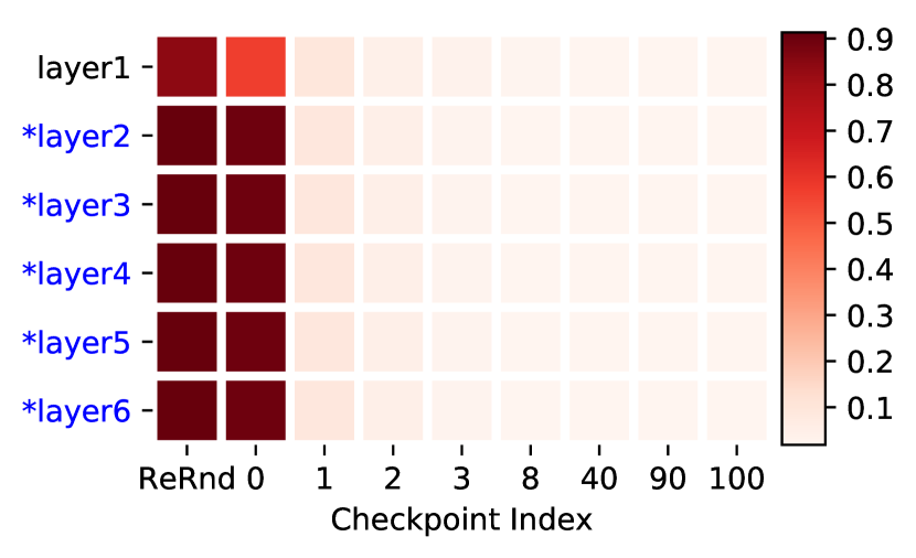
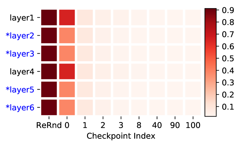



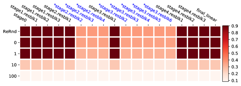


In this appendix, we provide results on joint robustness analysis that were not included in the main text due to space limit. From Sec. 3.1, we see that on MNIST, for wide enough FCNs, all the layers above layer1 are robust to re-initialization. So we divide the layers into two groups: {layer1} and {layer2, layer3, …}, and perform the robustness study on the two groups. The results for FCN are shown in Fig. 11(a). For clarity and ease of comparison, the figure still spells out all the layers individually, but the values from layer2 to layer6 are simply repeated rows. The values show that the upper-layer-group is clearly not jointly robust to re-initialization (to checkpoint-0).
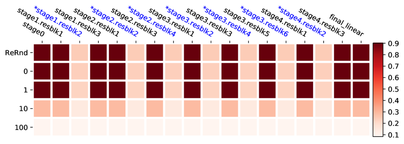
We also try some alternative grouping schemes: Fig. 11(b) show the results when we group two in every three layers, which has slightly improved joint robustness. In Fig. 11(c), the grouping scheme that includes every other layer shows that with a clever grouping scheme, about half of the layers could be jointly robust.
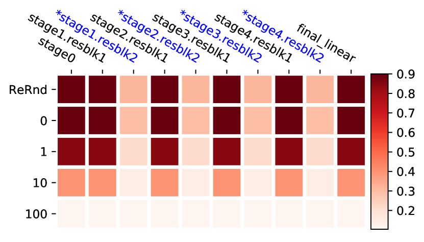
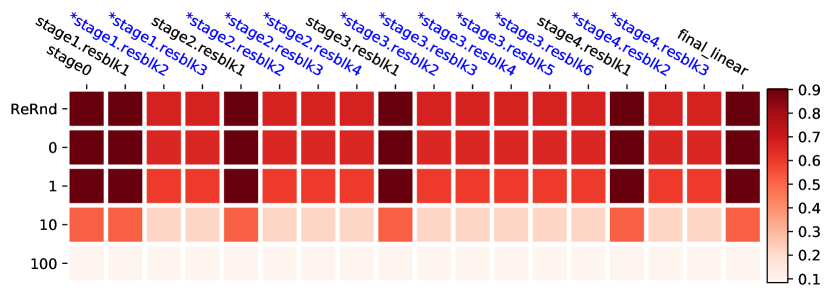
Results on ResNets are similar. Fig. 12 shows the joint robustness analysis on ResNets trained on CIFAR-10. The grouping is based on the individual layer robustness results from Fig. 4: all the residual blocks in stage1 to stage4 are bundled and analyzed jointly. The results are similar to the FCNs: ResNet-18 is relatively robust, but deeper ResNets are not jointly robust under this grouping. Two alternative grouping schemes are shown in Fig. 13. By including only layers from stage1 and stage4, slightly improved robustness could be obtained on ResNet-50. The scheme that groups every other residual block shows further improvements.
In summary, the individually robust layers are generally not jointly robust. But with some clever way of picking out a subset of the layers, joint robustness could still be achieved for up to half of the layers. In principle, one can enumerate all possible grouping schemes to find the best with a trade-off of the robustness and number of layers included.
Appendix C Batch Normalization and Weight Decay
The primary goal of this paper is to study the (co-)evolution of the representations at each layer during training and the robustness of this representation with respect to the rest of the network. We try to minimize the factors that explicitly encourage changing of the network weights or representations in the analysis. In particular, unless otherwise specified, weight decay and batch normalization were not used. This leads to some performance drop in the trained models. Especially for deep residual networks on ImageNet: even though we could successfully train a residual network with 100+ layers without batch normalization, the final generalization performance could be quite worse than the state-of-the-art. Therefore, in this section, we include experiments with networks trained with weight decay and batch normalization for comparison.
| Architecture | N/A | +wd | +bn | +wd+bn | |
|---|---|---|---|---|---|
| CIFAR-10 | ResNet-18 | 10.4 | 7.5 | 6.9 | 5.5 |
| ResNet-34 | 10.2 | 6.9 | 6.6 | 5.1 | |
| ResNet-50 | 8.4 | 9.9 | 7.6 | 5.0 | |
| ResNet-101 | 8.5 | 9.8 | 6.9 | 5.3 | |
| ResNet-152 | 8.5 | 9.7 | 7.3 | 4.7 | |
| VGG-11 | 11.8 | 10.7 | 9.4 | 8.2 | |
| VGG-13 | 10.3 | 8.8 | 8.4 | 6.7 | |
| VGG-16 | 11.0 | 11.4 | 8.5 | 6.7 | |
| VGG-19 | 12.1 | 8.6 | 6.9 | ||
| ImageNet | ResNet-18 | 41.1 | 33.1 | 33.5 | 31.5 |
| ResNet-34 | 39.9 | 30.6 | 30.1 | 27.2 | |
| ResNet-50 | 34.8 | 31.8 | 28.2 | 25.0 | |
| ResNet-101 | 32.9 | 29.9 | 26.9 | 22.9 | |
| ResNet-152 | 31.9 | 29.1 | 27.6 | 22.6 |
Table 3 shows the final test error rates of models trained with or without weight decay and batch normalization. Note the original VGG models do not use batch normalization (Simonyan and Zisserman, 2014), we list +bn variants here for comparison, by applying batch normalization to the output of each convolutional layer. On CIFAR-10, the performance gap varies from 3% to 5%, but on ImageNet, the gap could be as large as 10%.


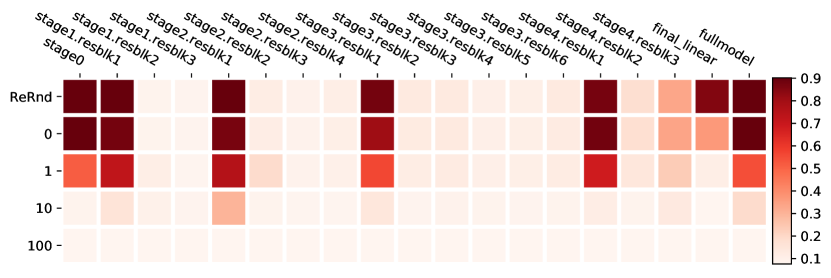
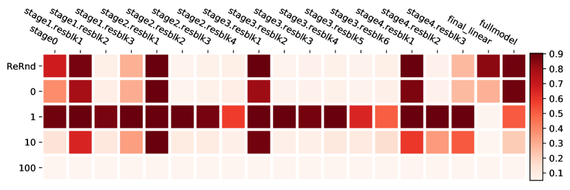
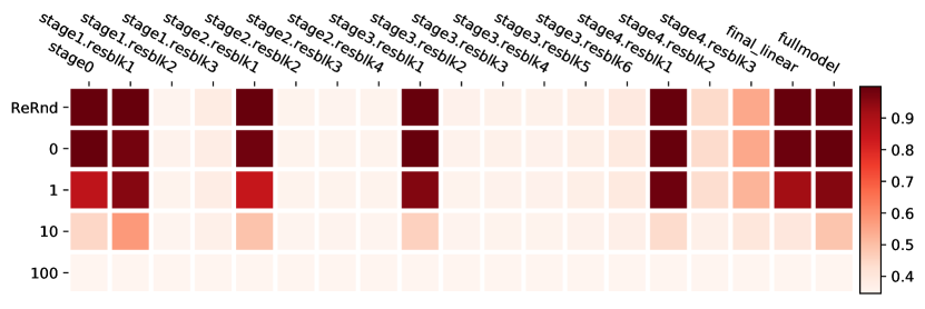
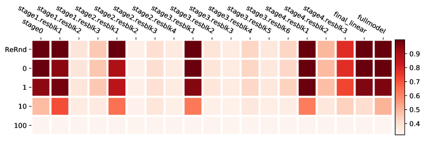


Fig. 14 shows how different training configurations affect the layer robustness analysis patterns on VGG-16 networks. Fig. 15 and Fig. 16 show similar comparisons for ResNet-50 on CIFAR-10 and ImageNet, respectively. We found that the layer robustness patterns are still quite pronounced under various training conditions. In Fig. 15(d) and Fig. 16(c,d), we found that re-initialing with checkpoint-1 is less robust than with checkpoint-0 for many layers. It might be that during early stages, some aggressive learning is causing changes in the parameters or statistics with large magnitudes, but later on when most of the training samples are classified correctly, the network gradually re-balances the layers to a more robust state. Fig. 18(d-f) in the next section show supportive evidence that, in this case the distance of the parameters between checkpoint-0 and checkpoint-1 is larger than between checkpoint-0 and the final checkpoint-T. However, on ImageNet this correlation is no longer clear as in Fig. 19(d-f). See also the discussions in the next section.
Appendix D Robustness and Distances
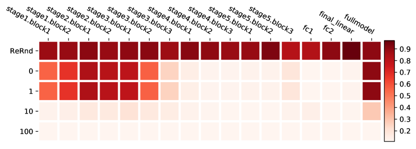
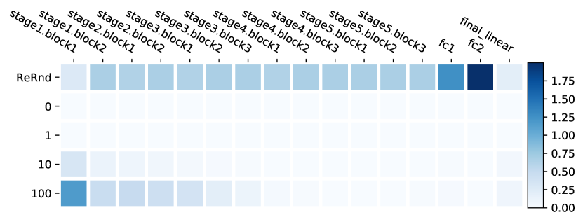
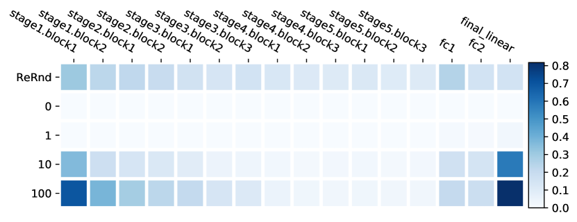
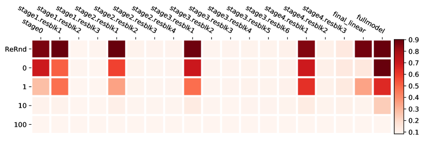

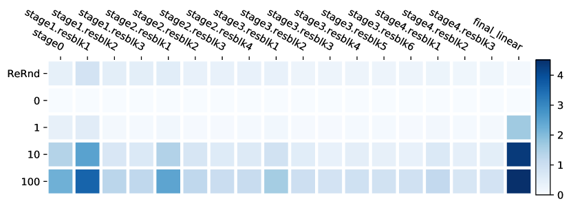

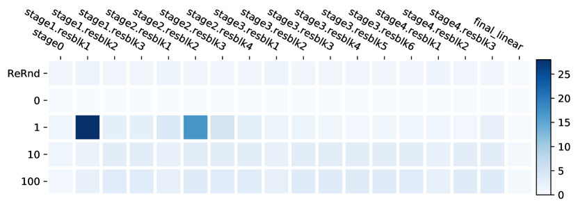


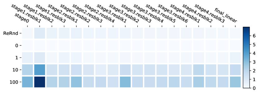
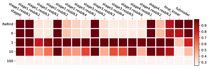
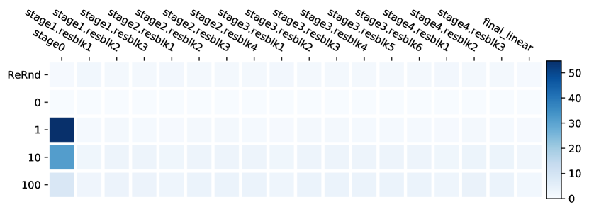
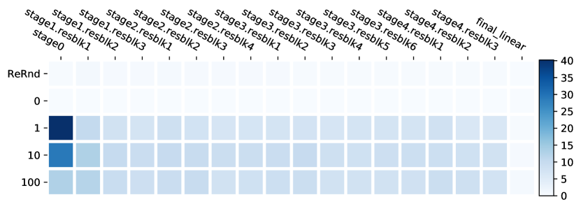
In Fig. 1 from Sec. 3.1, we compared the layer robustness patterns to the layer-wise distances of the parameters to the values at initialization (checkpoint-0). We found that for FCNs on MNIST, there is no obvious correlation between the “amount of parameter updates received” at each layer and its robustness to re-initialization for the two distances (the normalized and norms) we measured. In this appendix, we list results on other models and datasets studied in this paper for comparison.
Fig. 17 shows the layer robustness plot along with the layer-wise distance plots for VGG-16 trained on CIFAR-10. We found that the distance of the top layers are large, but the model is robust when we re-initialize those layers. However, the normalized distance seem to be correlated with the layer robustness patterns: the upper layers that are more robust moved smaller distances from their initialized values during training.
Similar plots for ResNet-50 on CIFAR-10 and ImageNet are shown in Fig. 18 and Fig. 19, respectively. In each of the figures, we also show extra results for models trained with weight decay and batch normalization. For the case without weight decay and batch normalization, we can see a weak correlation: the layers that are critical have slightly larger distances to their random initialization values. For the case with weight decay and batch normalization, the situation is less clear. First of all, in Fig. 18(e-f), we see very large distances in a few layers at checkpoint-1. This provides a potential explanation to the mysterious pattern that re-initialization to checkpoint-1 is more sensitive than to checkpoint-0. Similar observations can be found in Fig. 19(e-f) for ImageNet.
Appendix E Alternative Visualizations
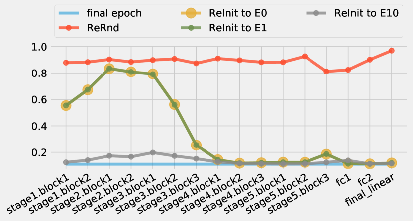
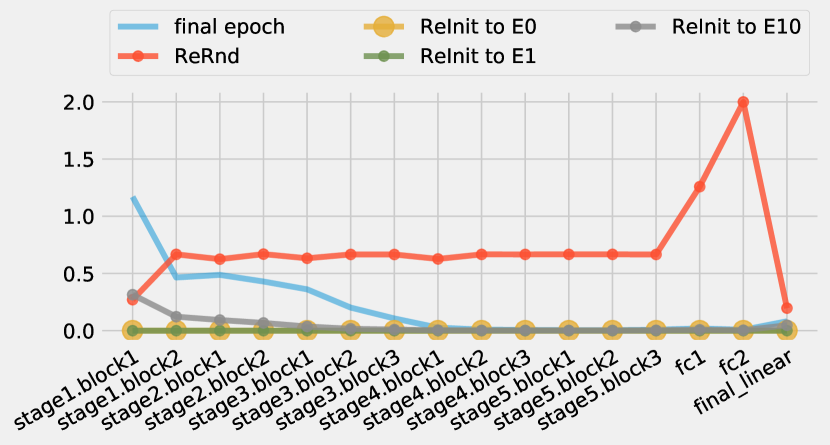
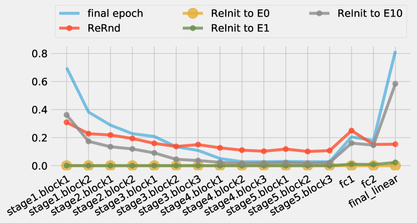

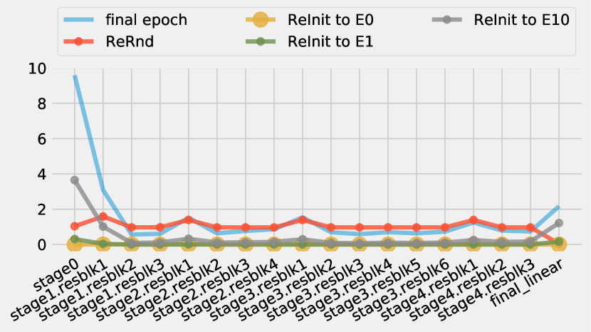
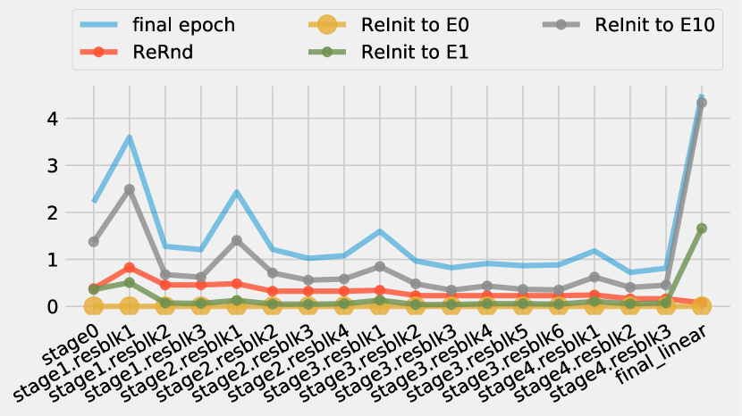
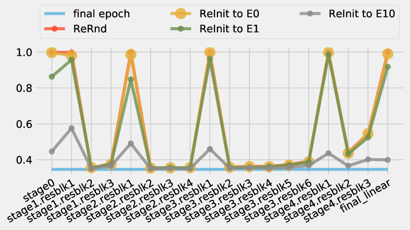


The empirical results on layer robustness are mainly visualized as heatmaps in the main text. The heatmaps allow uncluttered comparison of the results across layers and training epochs. However, it is not easy to tell the difference between numerical values that are close to each other from the color coding. In this section, we provide alternative visualizations that shows the same results with line plots. In particular, Fig. 20 shows the layer robustness analysis for VGG-16 on CIFAR-10. Fig. 21 shows the results for ResNet-50 on CIFAR-10 and ImageNet, respectively.
References
- Allen-Zhu et al. (2018) Zeyuan Allen-Zhu, Yuanzhi Li, and Zhao Song. A convergence theory for deep learning via Over-Parameterization. CoRR, arXiv:1811.03962, 2018.
- Anthony and Bartlett (2009) Martin Anthony and Peter L Bartlett. Neural Network Learning: Theoretical Foundations. Cambridge University Press, 2009.
- Arora et al. (2018) Sanjeev Arora, Rong Ge, Behnam Neyshabur, and Yi Zhang. Stronger generalization bounds for deep nets via a compression approach. CoRR, arXiv:1802.05296, 2018.
- Athalye et al. (2018) Anish Athalye, Nicholas Carlini, and David Wagner. Obfuscated gradients give a false sense of security: Circumventing defenses to adversarial examples. In International Conference on Machine Learning, pages 274–283. PMLR, 2018.
- Azizan et al. (2019) Navid Azizan, Sahin Lale, and Babak Hassibi. Stochastic mirror descent on overparameterized nonlinear models: Convergence, implicit regularization, and generalization. arXiv preprint arXiv:1906.03830, 2019.
- Ba et al. (2016) Jimmy Lei Ba, Jamie Ryan Kiros, and Geoffrey E Hinton. Layer normalization. arXiv preprint arXiv:1607.06450, 2016.
- Bartlett et al. (2017) Peter L Bartlett, Dylan J Foster, and Matus J Telgarsky. Spectrally-normalized margin bounds for neural networks. In Advances in Neural Information Processing Systems, pages 6240–6249, 2017.
- Belkin et al. (2018a) Mikhail Belkin, Daniel Hsu, Siyuan Ma, and Soumik Mandal. Reconciling modern machine learning and the bias-variance trade-off. arXiv preprint arXiv:1812.11118, 2018a.
- Belkin et al. (2018b) Mikhail Belkin, Daniel J Hsu, and Partha Mitra. Overfitting or perfect fitting? risk bounds for classification and regression rules that interpolate. In Advances in Neural Information Processing Systems, pages 2300–2311, 2018b.
- Belkin et al. (2018c) Mikhail Belkin, Siyuan Ma, and Soumik Mandal. To understand deep learning we need to understand kernel learning. arXiv preprint arXiv:1802.01396, 2018c.
- Chatterji et al. (2020) Niladri S Chatterji, Behnam Neyshabur, and Hanie Sedghi. The intriguing role of module criticality in the generalization of deep networks. In International Conference on Learning Representations, 2020.
- Chaudhari et al. (2017) Pratik Chaudhari, Anna Choromanska, Stefano Soatto, Yann LeCun, Carlo Baldassi, Christian Borgs, Jennifer Chayes, Levent Sagun, and Riccardo Zecchina. Entropy-sgd: Biasing gradient descent into wide valleys. In ICLR, 2017.
- Chelba et al. (2013) Ciprian Chelba, Tomas Mikolov, Mike Schuster, Qi Ge, Thorsten Brants, and Phillipp Koehn. One billion word benchmark for measuring progress in statistical language modeling. CoRR, abs/1312.3005, 2013. URL http://arxiv.org/abs/1312.3005.
- Cybenko (1989) G Cybenko. Approximation by superposition of sigmoidal functions. Mathematics of Control, Signals and Systems, 2(4):303–314, 1989.
- Daniely et al. (2016) Amit Daniely, Roy Frostig, and Yoram Singer. Toward deeper understanding of neural networks: The power of initialization and a dual view on expressivity. In Advances In Neural Information Processing Systems, pages 2253–2261, 2016.
- Delalleau and Bengio (2011) Olivier Delalleau and Yoshua Bengio. Shallow vs. Deep Sum-Product Networks. In NIPS, pages 666–674, 2011.
- Deng et al. (2009) Jia Deng, Wei Dong, Richard Socher, Li-Jia Li, Kai Li, and Li Fei-Fei. Imagenet: A large-scale hierarchical image database. In 2009 IEEE conference on computer vision and pattern recognition, pages 248–255. Ieee, 2009.
- Devroye et al. (2013) Luc Devroye, László Györfi, and Gábor Lugosi. A probabilistic theory of pattern recognition, volume 31. Springer Science & Business Media, 2013.
- Dosovitskiy et al. (2021) Alexey Dosovitskiy, Lucas Beyer, Alexander Kolesnikov, Dirk Weissenborn, Xiaohua Zhai, Thomas Unterthiner, Mostafa Dehghani, Matthias Minderer, Georg Heigold, Sylvain Gelly, Jakob Uszkoreit, and Neil Houlsby. An image is worth 16x16 words: Transformers for image recognition at scale. In International Conference on Learning Representations, 2021.
- Du et al. (2018a) Simon S Du, Jason D Lee, Haochuan Li, Liwei Wang, and Xiyu Zhai. Gradient descent finds global minima of deep neural networks. CoRR, arXiv:1811.03804, 2018a.
- Du et al. (2018b) Simon S Du, Xiyu Zhai, Barnabas Poczos, and Aarti Singh. Gradient descent provably optimizes over-parameterized neural networks. CoRR, arXiv:1810.02054, 2018b.
- Dziugaite and Roy (2017) Gintare Karolina Dziugaite and Daniel M Roy. Computing nonvacuous generalization bounds for deep (stochastic) neural networks with many more parameters than training data. In UAI, 2017.
- Eldan and Shamir (2015) Ronen Eldan and Ohad Shamir. The Power of Depth for Feedforward Neural Networks. CoRR, arXiv:1512.03965, 2015.
- Foret et al. (2021) Pierre Foret, Ariel Kleiner, Hossein Mobahi, and Behnam Neyshabur. Sharpness-aware minimization for efficiently improving generalization. In International Conference on Learning Representations, 2021.
- Goodfellow et al. (2014) Ian J Goodfellow, Jonathon Shlens, and Christian Szegedy. Explaining and harnessing adversarial examples. CoRR, arXiv:1412.6572, 2014.
- Györfi et al. (2006) László Györfi, Michael Kohler, Adam Krzyzak, and Harro Walk. A distribution-free theory of nonparametric regression. Springer Science & Business Media, 2006.
- Han et al. (2015) Song Han, Huizi Mao, and William J Dally. Deep compression: Compressing deep neural networks with pruning, trained quantization and huffman coding. CoRR, arXiv:1510.00149, 2015.
- Hardt and Ma (2017) Moritz Hardt and Tengyu Ma. Identity matters in deep learning. In ICLR, 2017.
- He et al. (2016a) Kaiming He, Xiangyu Zhang, Shaoqing Ren, and Jian Sun. Deep residual learning for image recognition. In Proceedings of the IEEE conference on computer vision and pattern recognition, pages 770–778, 2016a.
- He et al. (2016b) Kaiming He, Xiangyu Zhang, Shaoqing Ren, and Jian Sun. Identity mappings in deep residual networks. In European conference on computer vision, pages 630–645. Springer, 2016b.
- Hinton et al. (2015) Geoffrey Hinton, Oriol Vinyals, and Jeff Dean. Distilling the knowledge in a neural network. CoRR, arXiv:1503.02531, 2015.
- Hochreiter and Schmidhuber (1997) Sepp Hochreiter and Jürgen Schmidhuber. Flat minima. Neural Computation, 9(1):1–42, 1997.
- Hornik (1991) Kurt Hornik. Approximation capabilities of multilayer feedforward networks. Neural networks, 4(2):251–257, 1991.
- Hornik et al. (1989) Kurt Hornik, Maxwell Stinchcombe, and Halbert White. Multilayer feedforward networks are universal approximators. Neural networks, 2(5):359–366, 1989.
- Jacot et al. (2018) Arthur Jacot, Franck Gabriel, and Clément Hongler. Neural tangent kernel: Convergence and generalization in neural networks. In Advances in neural information processing systems, pages 8580–8589, 2018.
- Kawaguchi et al. (2017) Kenji Kawaguchi, Leslie Pack Kaelbling, and Yoshua Bengio. Generalization in deep learning. CoRR, arXiv:1710.05468, 2017.
- Keskar et al. (2017) Nitish Shirish Keskar, Dheevatsa Mudigere, Jorge Nocedal, Mikhail Smelyanskiy, and Ping Tak Peter Tang. On large-batch training for deep learning: Generalization gap and sharp minima. In ICLR, 2017.
- Kingma and Ba (2015) Diederik P Kingma and Jimmy Ba. Adam: A method for stochastic optimization. In International Conference on Learning Representations, 2015.
- Lee et al. (2019) Jaehoon Lee, Lechao Xiao, Samuel S Schoenholz, Yasaman Bahri, Jascha Sohl-Dickstein, and Jeffrey Pennington. Wide neural networks of any depth evolve as linear models under gradient descent. arXiv preprint arXiv:1902.06720, 2019.
- Liang et al. (2017) Tengyuan Liang, Tomaso Poggio, Alexander Rakhlin, and James Stokes. Fisher-rao metric, geometry, and complexity of neural networks. CoRR, arXiv:1711.01530, 2017.
- Liu et al. (2018) Peter J Liu, Mohammad Saleh, Etienne Pot, Ben Goodrich, Ryan Sepassi, Lukasz Kaiser, and Noam Shazeer. Generating wikipedia by summarizing long sequences. In International Conference on Learning Representations, 2018.
- Madry et al. (2017) Aleksander Madry, Aleksandar Makelov, Ludwig Schmidt, Dimitris Tsipras, and Adrian Vladu. Towards deep learning models resistant to adversarial attacks. CoRR, arXiv:1706.06083, 2017.
- Mhaskar and Poggio (2016) Hrushikesh Mhaskar and Tomaso A. Poggio. Deep vs. shallow networks : An approximation theory perspective. CoRR, arXiv:1608.03287, 2016.
- Montufar et al. (2014) Guido F Montufar, Razvan Pascanu, Kyunghyun Cho, and Yoshua Bengio. On the number of linear regions of deep neural networks. In Advances in neural information processing systems (NIPS), pages 2924–2932, 2014.
- Neyshabur et al. (2017) Behnam Neyshabur, Srinadh Bhojanapalli, David McAllester, and Nati Srebro. Exploring generalization in deep learning. In Advances in Neural Information Processing Systems, pages 5947–5956, 2017.
- Neyshabur et al. (2018) Behnam Neyshabur, Srinadh Bhojanapalli, and Nathan Srebro. A PAC-Bayesian approach to Spectrally-Normalized margin bounds for neural networks. In ICLR, 2018.
- Nguyen and Hein (2018) Quynh Nguyen and Matthias Hein. Optimization Landscape and Expressivity of Deep CNNs. In International Conference on Machine Learning, pages 3727–3736, 2018.
- Pinkus (1999) Allan Pinkus. Approximation theory of the MLP model in neural networks. Acta Numerica, 8:143–195, 1999.
- Poggio et al. (2018) Tomaso Poggio, Qianli Liao, Brando Miranda, Andrzej Banburski, Xavier Boix, and Jack Hidary. Theory iiib: Generalization in deep networks. Technical report, MIT, 2018.
- Raffel et al. (2020) Colin Raffel, Noam Shazeer, Adam Roberts, Katherine Lee, Sharan Narang, Michael Matena, Yanqi Zhou, Wei Li, and Peter J. Liu. Exploring the limits of transfer learning with a unified text-to-text transformer. Journal of Machine Learning Research, 21(140):1–67, 2020. URL http://jmlr.org/papers/v21/20-074.html.
- Rahimi and Recht (2008) Ali Rahimi and Benjamin Recht. Random features for large-scale kernel machines. In Advances in neural information processing systems, pages 1177–1184, 2008.
- Rahimi and Recht (2009) Ali Rahimi and Benjamin Recht. Weighted sums of random kitchen sinks: Replacing minimization with randomization in learning. In Advances in neural information processing systems, pages 1313–1320, 2009.
- Rivasplata et al. (2019) Omar Rivasplata, Vikram M Tankasali, and Csaba Szepesvari. Pac-bayes with backprop. arXiv preprint arXiv:1908.07380, 2019.
- Rolnick and Tegmark (2017) David Rolnick and Max Tegmark. The power of deeper networks for expressing natural functions. CoRR, arXiv:1705.05502, 2017.
- Rosenfeld and Tsotsos (2018) Amir Rosenfeld and John K Tsotsos. Intriguing Properties of Randomly Weighted Networks: Generalizing While Learning Next to Nothing. CoRR, arXiv:1802.00844, 2018.
- Shaham et al. (2015) Uri Shaham, Alexander Cloninger, and Ronald R Coifman. Provable approximation properties for deep neural networks. CoRR, arXiv:1509.07385, 2015.
- Simonyan and Zisserman (2014) Karen Simonyan and Andrew Zisserman. Very deep convolutional networks for large-scale image recognition. arXiv preprint arXiv:1409.1556, 2014.
- Smith and Le (2018) Samuel L Smith and Quoc V Le. A bayesian perspective on generalization and stochastic gradient descent. In ICLR, 2018.
- Szegedy et al. (2013) Christian Szegedy, Wojciech Zaremba, Ilya Sutskever, Joan Bruna, Dumitru Erhan, Ian Goodfellow, and Rob Fergus. Intriguing properties of neural networks. CoRR, arXiv:1312.6199, 2013.
- Telgarsky (2016) Matus Telgarsky. benefits of depth in neural networks. In Vitaly Feldman, Alexander Rakhlin, and Ohad Shamir, editors, 29th Annual Conference on Learning Theory, volume 49 of Proceedings of Machine Learning Research, pages 1517–1539, Columbia University, New York, New York, USA, 23–26 Jun 2016. PMLR.
- Tolstikhin et al. (2021) Ilya O Tolstikhin, Neil Houlsby, Alexander Kolesnikov, Lucas Beyer, Xiaohua Zhai, Thomas Unterthiner, Jessica Yung, Andreas Steiner, Daniel Keysers, Jakob Uszkoreit, et al. Mlp-mixer: An all-mlp architecture for vision. In Advances in Neural Information Processing Systems, volume 34, 2021.
- Vaswani et al. (2017) Ashish Vaswani, Noam Shazeer, Niki Parmar, Jakob Uszkoreit, Llion Jones, Aidan N Gomez, Łukasz Kaiser, and Illia Polosukhin. Attention is all you need. Advances in neural information processing systems, 30, 2017.
- Veit et al. (2016) Andreas Veit, Michael J Wilber, and Serge Belongie. Residual networks behave like ensembles of relatively shallow networks. In Advances in Neural Information Processing Systems, pages 550–558, 2016.
- Yun et al. (2018) Chulhee Yun, Suvrit Sra, and Ali Jadbabaie. Finite sample expressive power of small-width relu networks. CoRR, arXiv:1810.07770, 2018.
- Zhang et al. (2017) Chiyuan Zhang, Samy Bengio, Moritz Hardt, Benjamin Recht, and Oriol Vinyals. Understanding deep learning requires rethinking generalization. In ICLR, 2017.
- Zhou et al. (2019) Wenda Zhou, Victor Veitch, Morgane Austern, Ryan P Adams, and Peter Orbanz. Non-vacuous generalization bounds at the ImageNet scale: a PAC-Bayesian compression approach. In ICLR, 2019.
- Zou et al. (2018) Difan Zou, Yuan Cao, Dongruo Zhou, and Quanquan Gu. Stochastic gradient descent optimizes over-parameterized deep ReLU networks. CoRR, arXiv:1811.08888, 2018.