Semi-supervised learning via Feedforward-Designed
Convolutional Neural Networks

Abstract

A semi-supervised learning framework using the feedforward-designed convolutional neural networks (FF-CNNs) is proposed for image classification in this work. One unique property of FF-CNNs is that no backpropagation is used in model parameters determination. Since unlabeled data may not always enhance semi-supervised learning [1], we define an effective quality score and use it to select a subset of unlabeled data in the training process. We conduct experiments on the MNIST, SVHN, and CIFAR-10 datasets, and show that the proposed semi-supervised FF-CNN solution outperforms the CNN trained by backpropagation (BP-CNN) when the amount of labeled data is reduced. Furthermore, we develop an ensemble system that combines the output decision vectors of different semi-supervised FF-CNNs to boost classification accuracy. The ensemble systems can achieve further performance gains on all three benchmarking datasets.

Index Terms—  Semi-supervised learning, Ensemble, Image classification, Interpretable CNN

1 Introduction

When there are no sufficient labeled data available, we need to resort to semi-supervised learning (SSL) in tackling machine learning problems. SSL is essential in real world applications, where labeling is expensive and time-consuming. It attempts to boost the performance by leveraging unlabeled data. Its main challenge is how to use unlabeled data effectively to enhance decision boundaries that have been obtained by a small amount of labeled data. Convolutional neural networks (CNNs) are typically a fully-supervised learning tool since they demand a large amount of labeled data to represent the cost function accurately. As the amount of labeled data is small, the cost function is less accurate and, thus, it is not easy to formulate an SSL framework using CNNs.

Model parameters of CNNs are traditionally trained under a certain optimization framework with the backpropagation (BP) algorithm. They are called BP-CNNs. Recently, a feedforward-designed convolutional neural network (FF-CNN) methodology was proposed by Kuo et al. [2]. The model parameters of FF-CNNs at a target layer are determined by statistics of the output from its previous layer. Neither an optimization framework nor the BP training algorithm is utilized. Clearly, FF-CNNs are less dependent on data labels. We propose an SSL system based on FF-CNNs in this work.

This work has several novel contributions. First, we apply FF-CNNs to the SSL context and show that FF-CNNs outperforms BP-CNNs when the size of the labeled data set becomes smaller. Second, we propose an ensemble system that fuses the output decision vectors of multiple FF-CNNs so as to achieve even better performance. Third, we conduct experiments in three benchmarking datasets (i.e., MNIST, SVHN, and CIFAR-10) to demonstrate the effectiveness of the proposed solutions as described above.

The rest of this work is organized as follows. Both SSL and FF-CNN are reviewed in Sec. 2. The proposed SSL solutions using a single FF-CNN and ensembles of multiple FF-CNNs are described in Sec. 3. Experimental results are shown in Sec.4. Finally, concluding remarks are drawn and future work is discussed in Sec. 5.

2 Review of Related Work

Semi-Supervised Learning (SSL). There are several well-known SSL methods proposed in the literature. Iterative learning, including self-training [3] and co-training [4], learns from unlabeled data that have high confidence predictions. Transductive SVMs [5] extend standard SVMs by maximizing the margin on unlabeled data as well. Another SSL method is to construct a graph to represent data structures and propagate the label information of a labeled data point to unlabeled ones [6, 7]. More recently, several SSL methods are proposed based on deep generative models, such as the variational auto-encoder (VAE) [8], and generative adversarial networks (GAN) [9, 10]. All parameters in these networks are determined by the stochastic gradient descent (SGD) algorithm through BP and they are trained based on both labeled and unlabeled data.

Feedforward-designed CNNs (FF-CNNs). The BP training is computationally intensive, and the learning model of a BP-CNN is lack of interpretability. New solutions have been proposed to tackle these issues. Examples include: interpretable CNNs [11, 12, 13] and feedforward-designed CNNs (FF-CNNs) [14, 15, 2]. FF-CNNs contain two modules: 1) construction of convolutional (conv) layers through subspace approximations, and 2) construction of fully-connected (FC) layers via training sample clustering and least-squared regression (LSR). They are elaborated below.

The construction of conv layers is realized by multi-stage Saab transforms [2]. The Saab transform is a variant of the principal component analysis (PCA) with a constant bias vector to annihilate activation’s nonlinearity. The Saab transform can reduce feature redundancy in the spectral domain, yet there still exists correlation among spatial dimensions of the same spectral component. This is especially true in low-frequency spectral components. Thus, a channel-wise PCA (C-PCA) was proposed in [16] to reduce spatial redundancy of Saab coefficients furthermore. Since the construction of conv layers is unsupervised, they can be fully adopted in an SSL system.

The construction of FC layers is achieved by the cascade of multiple rectified linear least-squared regressors (LSRs) [2]. Let the input and output dimensions of a FC layer be $N_{in}$ and $N_{out}$ (with $N_{in}>N_{out}$), respectively. To construct an FC layer, we cluster input samples of dimension $N_{in}$ into $N_{out}$ clusters, and assign pseudo-labels based on clustering results. Next, all samples are transformed into a vector space of dimension $N_{out}$ via LSR, where the index of the output space dimension defines a pseudo-label. In this way, we obtain a supervised LSR building module to serve as one FC layer. It accommodates intra-class variability while enhancing discriminability gradually.

3 Proposed Methods

3.1 Semi-supervised Learning System

Problem Formulation and Data Pre-processing. The semi-supervised classification problem can be defined as follows. We have a set of $M$ unlabeled samples

$${\bf X}^{ul}=\{{\bf x}^{ul}_{1},\cdots,{\bf x}^{ul}_{M}\},$$

where ${\bf x}^{ul}_{i}\in\mathbb{R}^{D_{in}}$ is the $i$th input unlabeled sample, and a set of labeled samples that can be written in form of pairs:

$$({\bf X}^{l},{\bf Y}^{l})=\{({\bf x}^{l}_{1},y^{l}_{1}),\cdots,({\bf x}^{l}_{N},y^{l}_{N}\},$$

where ${\bf x}^{l}_{i}\in\mathbb{R}^{D_{in}}$ is the $i$th input labeled sample and $y_{i}^{l}\in\{1,\cdots,L\}$ is its class label. We omit index $i$ whenever the context is clear.

We adopt the multi-stage Saab transforms and C-PCA for unsupervised image feature extraction. They can be expressed as

$${\bf z}^{l}=T_{saab}({\bf x}^{l}),\mbox{ and }{\bf z}^{ul}=T_{saab}({\bf x}^{ul}),$$

where ${\bf z}^{l},{\bf z}^{ul}\in\mathbb{R}^{D_{out}}$, and $D_{in}>D_{out}$. This is used to facilitate classification with more powerful image features in a lower dimensional space.

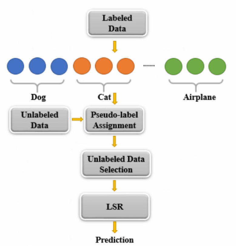
Fig. 1: The proposed semi-supervised learning (SSL) system.

Pseudo-Label Assignment. Next, we propose a semi-supervised method in the design of FC layers using multi-stage rectified LSRs as illustrated in Fig. 1. The pseudo-labels should be generated for both labeled and unlabeled samples in solving the LSR problem. To achieve this goal, we conduct K-means clustering on labeled samples of the same class. For example, we can cluster samples of a single original class into $M$ sub-classes to generate $M$ pseudo-categories. If there are $N$ original classes, we will generate $M\times N$ pseudo-categories in total. Then, pseudo-labels of labeled data can be generated by representing pseudo categories with one-hot vectors, denoted as

$${\bf Y}^{p}=\{{\bf y}^{p}_{1},\cdots,{\bf y}^{p}_{M}\}.$$

The centroid of the $j$th pseudo-category, denoted by $c_{j}$, provides a representative sample for the corresponding original class.

We define the probability vector of the pseudo-category for each unlabeled sample as

$$p(t_{k}|{\bf z}^{ul})=\frac{\alpha e^{{d_{k}}}}{\sum_{j}{\alpha e^{{d_{j}}}}};$$ (1)

where $t_{k}$ represents the $k$th pseudo-category and

$$d_{k}=\frac{{{\bf z}^{ul}}\cdot{\bf c}_{k}}{\|{\bf z}^{ul}\|\|{\bf c}_{k}\|}.$$ (2)

Then, the probability vector in (1) can be used as the pseudo-label of each unlabeled sample to set up a system of linear regression equations that relates the input data samples and pseudo-labels,

$$[{\bf Y}^{p},{\bf P}({\bf T}|{\bf Z}^{ul})]={\bf W}_{fc}[{\bf Z}^{l},{\bf Z}^{ul}],$$

where the parameters of FC layer are denoted by

$${\bf W}_{fc}={\bf(Z^{T}Z)^{-1}Z^{T}Y},$$ (3)

and where

$${\bf Z}=[{\bf Z}^{l},{\bf Z}^{ul}],\mbox{ and }{\bf Y}=[{\bf Y}^{p},{\bf P}({\bf T}|{\bf Z}^{ul})].$$ (4)

The final output of one-stage rectified LSR is

$${\bf z}^{l}_{out}=f({\bf W}_{fc}{\bf z}^{l})\mbox{ and }{\bf z}^{ul}_{out}=f({\bf W}_{fc}{\bf z}^{ul}),$$ (5)

where $f(.)$ is a non-linear activation function (e.g. ReLU in our experiments), and ${\bf z}^{l}_{out}$ and ${\bf z}^{ul}_{out}$ denote outputs of labeled and unlabeled data, respectively. The output vectors lie in a lower dimensional space. They are used as features to the next stage rectified LSR.

Unlabeled Sample Selection. Not every unlabeled sample is suitable for constructing FC layers. We define a quality score for each unlabeled sample ${\bf z}^{ul}$ as

$$S_{i}({\bf z}^{ul})=\frac{\sum_{k\in C_{i}}{p(t_{k}|{\bf z}^{ul})}}{\sum_{j}{p(t_{j}|{\bf z}^{ul})}},$$ (6)

where $C_{i}$ indicates a set of pseudo-categories that belong to the original $i$th class. A low qualify score indicates that the sample is far away from the representative set of examples of a single original class. We exclude those samples in solving the LSR problems.

Multi-stage LSRs. We repeat several LSRs and finally provide the predicted class labels. In the last stage, we cluster input data based on their original class labels and the LSR is solved using labeled samples only. The multi-stage setting is needed to remove feature redundancy in the spectral dimension and resolve intra-class variability gradually.

3.2 Ensembles

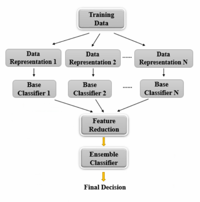
Fig. 2: An ensemble of multiple SSL decision systems.

Ensembles are often used to combine results from multiple weak classifiers to yield a stronger one [17]. We use the ensemble idea to achieve better performance in semi-supervised classification. Although both BP-CNNs and FF-CNNs can be improved by ensemble methods, FF-CNNs have much lower training complexity to justify an ensemble solution. The proposed ensemble system is illustrated in Fig. 2. Multiple semi-supervised FF-CNNs are adopted as the first-stage base classifiers in an ensemble system. Their output decision vectors are concatenated as new features. Afterwards, we apply the principal component analysis (PCA) technique to reduce feature dimension and then feed the dimension-reduced feature vector to the second-stage ensemble classifier.

High input diversity is essential to an effective ensemble system that can reach a higher performance gain [18, 19]. In the proposed ensemble system, we adopt three strategies to increase input diversity. First, we consider different filter sizes in the conv layers as illustrated in Table 1 since different filter sizes lead to different features at the output of the conv layer with different receptive fields. Second, we represent color images in different color spaces [20]. In the experiments, we choose the RGB, YCbCr and Lab color spaces and process three channels separately for the latter two color spaces. Third, we decompose images into a set of feature maps using the 3x3 Laws filters [21], where each feature map focuses on different characteristics of the input image (e.g., brightness, edginess, etc.)

Table 1: Network architectures with respect to different input types and different conv layer parameter settings. The second to fourth columns indicate inputs from MNIST, RGB inputs and the single channel inputs from SVHN and CIFAR-10, accordingly.

		Greyscale	RGB	Single Channel
FF-1	Conv1	5$\times$5$\times$1, 6	5$\times$5$\times$3, 32	5$\times$5$\times$1, 16
	Conv2	5$\times$5$\times$6, 16	5$\times$5$\times$32, 64	5$\times$5$\times$16, 32
FF-2	Conv1	3$\times$3$\times$1, 6	3$\times$3$\times$3, 24	3$\times$3$\times$1, 8
	Conv2	5$\times$5$\times$6, 16	5$\times$5$\times$24, 64	5$\times$5$\times$8, 32
FF-3	Conv1	5$\times$5$\times$1, 6	5$\times$5$\times$3, 32	5$\times$5$\times$1, 16
	Conv2	3$\times$3$\times$6, 16	3$\times$3$\times$32, 64	3$\times$3$\times$16, 32
FF-4	Conv1	3$\times$3$\times$1, 6	3$\times$3$\times$3, 24	3$\times$3$\times$1, 8
	Conv2	3$\times$3$\times$6, 16	3$\times$3$\times$24, 48	3$\times$3$\times$8, 24

4 Experimental Results

We conduct experiments on three popular datasets: MNIST [22], SVHN [23] and CIFAR-10 [24]. We randomly select a subset of labeled training data from them, and test the classification performance on the entire testing set. Each object class has the same number of labeled data to ensure balanced training. We adopt the LeNet-5 architecture [25] for the MNIST dataset. Since CIFAR-10 is a color image dataset, we increase the filter numbers of the first and the second conv layers and the first and the second FC layers to 32, 64, 200 and 100, respectively, by following [2]. The C-PCA is applied to the output of the second conv layer and the feature dimension per channel is reduced from 25 to 20 (for MNIST) or 15 (for SVHN) or 12 (for CIFAR-10). The probability vectors are computed using Eq. (1), where $\alpha$ is set to 50 for all three datasets.

The Radial Basis Function (RBF) SVM classifier is used as the second-stage classifier in the ensemble systems in all experiments. Before training the SVM classifier, PCA is applied to the cascaded decision vectors of first-stage classifiers. The reduced feature dimension is determined based on the correlation of decision vectors of base classifiers in an ensemble.

4.1 Individual Semi-Supervised FF-CNN

We compare the performance of the BP-CNN and the proposed semi-supervised FF-CNN on three benchmark datasets in Fig. 3. For MNIST and SVHN, 1/2, 1/4, 1/8, 1/16,1/32, 1/64, 1/128, 1/256, 1/512 of the entire labeled training set are randomly selected to train the networks. As to CIFAR-10, 1/2, 1/4, 1/8, 1/16,1/32, 1/64, 1/128, 1/256 of the whole labeled dataset are used to learn network parameters. We use the labeled data to train the BP-CNNs. We select unlabeled training data with quality scores of top 70%, 70% and 80% in MNIST, SVHN and CIFAR-10, respectively, in the training of the corresponding semi-supervised FF-CNN.

Table 2: Testing accuracy (%) comparison under three settings: 1) without using unlabeled data; 2) using the entire set of unlabeled data; and 3) using a subset of unlabeled data based on quality scores defined by Eq. (1). 1/256 of the labeled data is used on MNIST and SVHN datasets, and 1/128 of the labeled data is used on CIFAR-10 dataset.

	MNIST	SVHN	CIFAR-10
Setting 1	57.19 ($\pm$ 3.4)	25.17 ($\pm$ 1.10)	24.64 ($\pm$ 0.25)
Setting 2	92.26 ($\pm$ 0.33)	53.76 ($\pm$ 0.97)	41.95 ($\pm$ 0.56)
Setting 3	92.65 ($\pm$ 0.14)	58.58 ($\pm$ 0.78)	42.53 ($\pm$ 0.57)

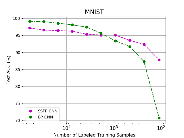
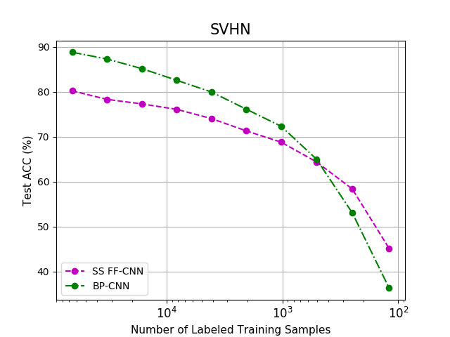
Fig. 3: The comparisons of testing accuracy (%) using BP-CNNs, and semi-supervised FF-CNNs on MNIST, SVHN and CIFAR-10 datasets, respectively.

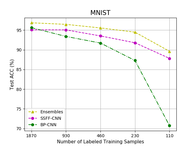
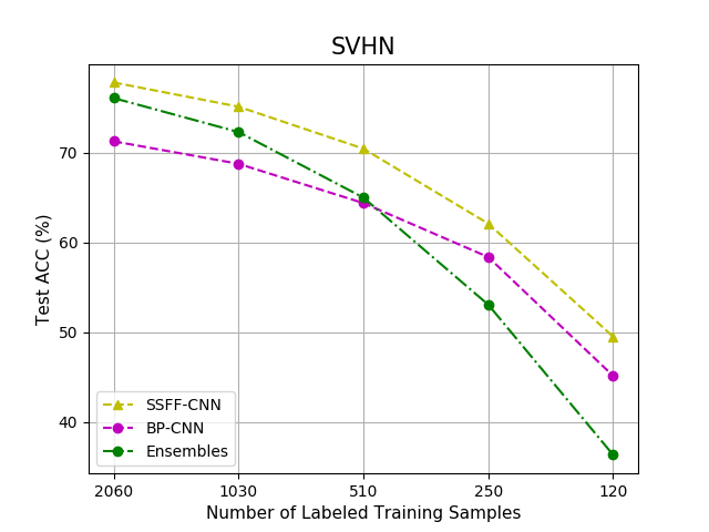
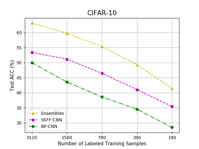
Fig. 4: The comparisons of testing accuracy (%) using BP-CNNs, semi-supervised FF-CNNs, and ensembles of semi-supervised FF-CNNs on the small labeled portion against MNIST, SVHN and CIFAR-10 datasets, respectively.

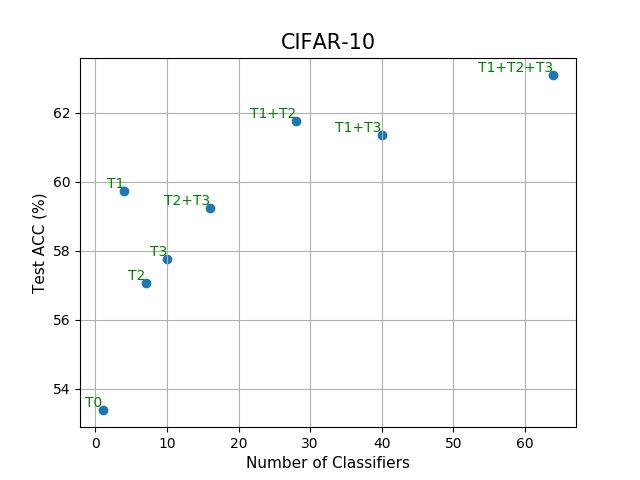
Fig. 5: The relation between test accuracy (%) and the number of semi-supervised FF-CNNs in the ensemble, where three diversity types are indicated as T1, T2 and T3, and T0 indicates the individual semi-supervised FF-CNN. The experiments are conducted on CIFAR-10 with 1/16 of the whole labels.

When using the entire labeled training set, the semi-supervised FF-CNN is exactly the same as the FF-CNN. There is a performance gap between FF-CNN and BP-CNN at the beginning of the plots. However, when the number of labeled training data is reduced, the performance degradation of the semi-supervised FF-CNN is not as severe as that of the BP-CNN and we see cross-over points between these two networks in all three datasets. For the extreme cases, we see that semi-supervised FF-CNNs outperform BP-CNNs by 17.1%, 8.8%, and 6.9% in testing accuracy with 110, 120, and 190 labeled data for MNIST, SVHN and CIFAR-10, respectively. The results show that the proposed semi-supervised FF-CNNs can learn from the unlabeled data more effectively than the corresponding BP-CNNs.

To evaluate the effectiveness of several unlabeled data usage ideas, we compare three different settings in Table 2. The best results come from using selected unlabeled training data. This is particularly obvious for the SVHN dataset. There is around 5% performance gain by eliminating low quality unlabeled samples.

4.2 Ensembles of Multiple Semi-Supervised FF-CNNs

The performance of the proposed ensemble system by fusing all diversity types is shown in Fig. 4. We see that ensembles can boost classification accuracy by a large gain. There are about 2%, 5% and 8% performance improvements against individual semi-supervised FF-CNNs, and the ensemble results with the smallest labeled portion achieve test accuracy of 89.6%, 49.5%, and 41.4% for MNIST, SVHN and CIFAR-10, respectively.

We further examine the performance of different diversity types, and show the relation between test accuracy and ensemble complexity in Fig. 5, where we test ensemble systems using different diversity types: 1) an ensemble of four semi-supervised FF-CNNs with varied filter sizes and filter numbers in two conv layers as listed in Table 1 (T1); 2) an ensemble of color input images in different color spaces (i.e. RGB, YCbCr, and Lab), where three channels separately for the latter two color spaces are treated separately (T2); and 3) an ensemble of nine semi-supervised FF-CNNs obtained by taking different input images computed from filtered greyscale images with 3x3 Laws filters [26] (T3).

As shown in the figure, the most efficient ensemble system among all designs is to fuse four different semi-supervised FF-CNNs with T1 diversity which yields a performance gain of 6.4%. In general, an ensemble of more semi-supervised FF-CNNs provides higher testing accuracy. The best performance achieved is 63.1% by combining all three diversity types. As compared with that of the single FF-CNN trained with all labeled data, the performance of the ensemble of semi-supervised FF-CNNs trained with 1/16 labeled data is only slightly lower by 0.6%.

5 Conclusion and future work

A semi-supervised learning framework using FF-CNNs for image classification was proposed. It was demonstrated by experimental results on three benchmark datasets (MNIST, SVHN, and CIFAR-10) that the semi-supervised FF-CNNs offer an effective solution. The ensembles of multiple semi-supervised FF-CNNs can boost the performance furthermore. Two extensions of this work are under current investigation. One is incremental learning. The other is decision fusion in the spatial domain. FF-CNNs provide a more convenient tool than the BP-CNN in both contexts. We will explore them furthermore in the near future.

References

- [1] Xiaojin Zhu, “Semi-supervised learning literature survey,” Computer Science, University of Wisconsin-Madison, vol. 2, no. 3, pp. 4, 2006.
- [2] C-C Jay Kuo, Min Zhang, Siyang Li, Jiali Duan, and Yueru Chen, “Interpretable convolutional neural networks via feedforward design,” arXiv preprint arXiv:1810.02786, 2018.
- [3] Chuck Rosenberg, Martial Hebert, and Henry Schneiderman, “Semi-supervised self-training of object detection models.,” WACV/MOTION, vol. 2, 2005.
- [4] Avrim Blum and Tom Mitchell, “Combining labeled and unlabeled data with co-training,” in Proceedings of the eleventh annual conference on Computational learning theory. ACM, 1998, pp. 92–100.
- [5] Thorsten Joachims, “Transductive inference for text classification using support vector machines,” in ICML, 1999, vol. 99, pp. 200–209.
- [6] Xiaojin Zhu and Zoubin Ghahramani, “Learning from labeled and unlabeled data with label propagation,” Tech. Rep. CMU-CALD-02-107, Carnegie Mellon University, 2002.
- [7] Avrim Blum, John Lafferty, Mugizi Robert Rwebangira, and Rajashekar Reddy, “Semi-supervised learning using randomized mincuts,” in Proceedings of the twenty-first international conference on Machine learning. ACM, 2004, p. 13.
- [8] Durk P Kingma, Shakir Mohamed, Danilo Jimenez Rezende, and Max Welling, “Semi-supervised learning with deep generative models,” in Advances in neural information processing systems, 2014, pp. 3581–3589.
- [9] Zihang Dai, Zhilin Yang, Fan Yang, William W Cohen, and Ruslan R Salakhutdinov, “Good semi-supervised learning that requires a bad gan,” in Advances in Neural Information Processing Systems, 2017, pp. 6510–6520.
- [10] Tim Salimans, Ian Goodfellow, Wojciech Zaremba, Vicki Cheung, Alec Radford, and Xi Chen, “Improved techniques for training gans,” in Advances in Neural Information Processing Systems, 2016, pp. 2234–2242.
- [11] Quanshi Zhang, Ying Nian Wu, and Song-Chun Zhu, “Interpretable convolutional neural networks,” arXiv preprint arXiv:1710.00935, 2017.
- [12] C.-C. Jay Kuo, “Understanding convolutional neural networks with a mathematical model,” Journal of Visual Communication and Image Representation, vol. 41, pp. 406–413, 2016.
- [13] C.-C. Jay Kuo, “The CNN as a guided multilayer RECOS transform [lecture notes],” IEEE Signal Processing Magazine, vol. 34, no. 3, pp. 81–89, 2017.
- [14] Yueru Chen, Zhuwei Xu, Shanshan Cai, Yujian Lang, and C.-C. Jay Kuo, “A saak transform approach to efficient, scalable and robust handwritten digits recognition,” arXiv preprint arXiv:1710.10714, 2017.
- [15] C.-C. Jay Kuo and Yueru Chen, “On data-driven Saak transform,” Journal of Visual Communication and Image Representation, vol. 50, pp. 237–246, 2018.
- [16] Yueru Chen, Yijing Yang, Wei Wang, and C-C Jay Kuo, “Ensembles of feedforward-designed convolutional neural networks,” arXiv preprint arXiv:1901.02154, 2019.
- [17] Cha Zhang and Yunqian Ma, Ensemble machine learning: methods and applications, Springer, 2012.
- [18] Gavin Brown, Jeremy Wyatt, Rachel Harris, and Xin Yao, “Diversity creation methods: a survey and categorisation,” Information Fusion, vol. 6, no. 1, pp. 5–20, 2005.
- [19] Ludmila I Kuncheva and Christopher J Whitaker, “Measures of diversity in classifier ensembles and their relationship with the ensemble accuracy,” Machine learning, vol. 51, no. 2, pp. 181–207, 2003.
- [20] Noor A Ibraheem, Mokhtar M Hasan, Rafiqul Z Khan, and Pramod K Mishra, “Understanding color models: a review,” ARPN Journal of science and technology, vol. 2, no. 3, pp. 265–275, 2012.
- [21] Kenneth I Laws, “Rapid texture identification,” in Image processing for missile guidance. International Society for Optics and Photonics, 1980, vol. 238, pp. 376–382.
- [22] Yann LeCun, Léon Bottou, Yoshua Bengio, and Patrick Haffner, “Gradient-based learning applied to document recognition,” Proceedings of the IEEE, vol. 86, no. 11, pp. 2278–2324, 1998.
- [23] Yuval Netzer, Tao Wang, Adam Coates, Alessandro Bissacco, Bo Wu, and Andrew Y Ng, “Reading digits in natural images with unsupervised feature learning,” in NIPS workshop on deep learning and unsupervised feature learning, 2011, vol. 2011, p. 5.
- [24] Alex Krizhevsky and Geoffrey Hinton, “Learning multiple layers of features from tiny images,” Tech. Rep., Citeseer, 2009.
- [25] Yann Lecun, Léon Bottou, Yoshua Bengio, and Patrick Haffner, “Gradient-based learning applied to document recognition,” in Proceedings of the IEEE, 1998, pp. 2278–2324.
- [26] William K Pratt, Digital image processing: PIKS Scientific inside, vol. 4, Wiley-interscience Hoboken, New Jersey, 2007.