Spectroscopy of double quantum dot two-spin states by tuning the inter-dot barrier
Abstract
Transport spectroscopy of two-spin states in a double quantum dot can be performed by an AC electric field which tunes the energy detuning. However, a problem arises when the transition rate between the states is small and, consequently, the AC-induced current is suppressed. Here, we show that if the AC field tunes the inter-dot tunnel barrier then for large detuning the transition rate increases drastically resulting in high current. Multi-photon resonances are enhanced by orders of magnitude. Our study demonstrates an efficient way for fast two-spin transitions.
I Introduction
A double quantum dot containing two electron spins can be used for the realization of two-qubit operations. hanson07 ; zwanenburg13 ; petta05 ; loss98 ; brunner11 ; pioro08 This qubit system is attractive because it is tunable by applying appropriate voltages to surface gate electrodes. hanson07 ; zwanenburg13 Information on the coupled spin-qubits can be extracted by electrical transport techniques. hanson07 ; zwanenburg13 It has been demonstrated that in double dots with spin-orbit interaction (SOI) transitions between the two-spin eigenstates can be induced by applying an AC electric field to a gate electrode. perge12 ; stehlik14 ; ono17 In essence the AC field changes periodically the energy detuning of the double dot, and the transitions give rise to current peaks when the condition is satisfied. The energy splitting of the relevant double dot eigenstates is , the AC frequency is , Planck’s constant is , and the integer denotes the ‘-photon’ resonance. This process enables spectroscopy of the spin states by measuring the current as a function of the AC field frequency and magnetic field. perge12 ; stehlik14 ; ono17
The amplitude of the AC electric field is an important parameter, because if it is small the transitions are slow and, consequently the AC-induced current peaks are suppressed and eventually cannot be probed. This is more evident for the peaks corresponding to -photon resonances () which are usually visible only when the AC field amplitude is large. stehlik14 ; ono17 However, generating a large AC amplitude is a challenging task. wiel02 This is one of the basic reasons that -photon resonances are not well studied in semiconductor quantum dot systems.
In this work, we consider a double dot (DD) in the regime of spin selective inter-dot tunneling, ono00 and in the presence of an AC electric field. We focus on two SOI-coupled eigenstates, and show that when the AC field tunes the inter-dot tunnel coupling (barrier) the singlet-triplet com1 transitions can be over an order of magnitude faster compared to those induced when the AC field tunes the energy detuning. This speedup is attractive for spin-qubit applications where fast operations are needed. The long time scale difference has a strong impact on the AC-induced current peaks. Specifically, the -photon resonances which are usually suppressed and are more difficult to probe are enhanced by orders of magnitude. As a result, the required AC field amplitude can be smaller.
Understanding the effect of tuning periodically the tunnel coupling of a DD is important from a more general perspective. In impurity-based DDs such that formed, for example, in silicon field-effect-transistors, ono17 ; ono18 the position of the dots inside the channel is unknown and the effect of applying an AC field to a gate electrode on the dot potential is unclear. The AC field can modulate the energy detuning and/or the inter-dot tunnel coupling. This scenario has also been suggested in gated quantum dots hanson07 ; zwanenburg13 ; nakajima18 , while control over the inter-dot tunnel coupling has been explored in various experiments. diepen18 ; mukhopa18 ; martins16 ; reed16
II Double dot Hamiltonian
We define the triplet states as well as the singlet states where () indicates the number of electrons on dot 1 (dot 2). The DD is described by the Hamiltonian
The Zeeman term is , with , the tunnel coupling is , the spin-flip tunnel coupling due to the SOI is , and the detuning is . We consider two SOI-coupled eigenstates and demonstrate that by tuning the inter-dot tunnel coupling with an AC field creates strong -photon current peaks which allow for spectroscopy of these eigenstates at smaller AC frequencies. We prove the efficacy of this process through a comparison with the case where the AC field tunes the energy detuning. Below we address two separate cases. In the first case, the detuning is time periodic due to the AC field
The second term accounts for the AC field which has amplitude and frequency . In the first case, the tunnel-couplings are constant in time and . In the second case, the AC field tunes the tunnel barrier, thus, the tunnel couplings are
In the second case, the energy detuning is constant in time . Some experiments ono17 ; stehlik14 ; chorley11 have demonstrated that and we assume that the AC field satisfies this condition and take , so the ratio is constant in time. To compare theoretically the two cases we assume the same amplitude and only briefly consider different amplitudes. In the experiment the required gate voltage to generate can be different for the two cases and sensitive to many factors, such as, the geometry of the DD, the electrode design, as well as the material, and screening effects.

III Singlet-triplet transitions
We focus on the two lowest eigenstates of the time independent part of , , , 2, and refer to as singlet and triplet eigenstates. The eigenenergies shown in Fig. 1 (upper frames) anticross due to the SOI; specifically we take T, and plot , versus for meV, and also plot , versus for meV [Ref. extranote, ]. Hereafter, we fix meV, meV and study first the coherent transitions between and , when the DD is not coupled to the leads. We express the time evolution of the DD state as follows
where the parameters are determined by the initial condition. The Floquet modes , and Floquet energies satisfy the Floquet eigenvalue problem . This is written in a simple form using Fourier expansion by noting that the Floquet modes have the same periodicity as that of the AC field, i.e., , , and the Floquet energies can be defined within the energy interval . The Floquet problem is reduced to a matrix eigenvalue problem and is solved numerically.
Figure 1 shows the transition probability , for T, eV, meV, and , , 2. This set of parameters does not lead to Landau-Zener dynamics, as that studied in Ref. stehlik16, , because the system is not driven through the anticrossing point. This is inferred directly from the dependence of , on the detuning and tunnel coupling (Fig. 1). When the AC field tunes the tunnel coupling the singlet-triplet transition for the single-photon resonance () is about 18 times faster compared to the case where the AC field tunes the detuning. Interestingly, for the two-photon resonance () the speedup is on the order of 300. In both cases the transitions are electrically driven mediated by the SOI.
In the weak driving regime transitions take place only between , and when the AC field tunes the tunnel coupling the dynamics is captured by the approximate Hamiltonian suppl . This model predicts the resonant transition probability , with
| (1) |
| (2) |
and is a Bessel function of the first kind, , 2, … denotes the ‘photon’ index. Likewise the case where the AC field tunes the energy detuning can be examined with the substitutions and , where
| (3) |
According to the approximate model the singlet-triplet transition times are quantified by the coupling constants , , and these can be very different. For example, if we focus on and when the argument of is very small [, ] then to a good approximation [Ref. absol, ]. For large negative detuning where the two spins are effectively in the Heisenberg regime , because the character dominates significantly over the , hence, near the anticrossing point , while the terms proportional to have negligible effect. Away from the anticrossing point the terms proportional to , need to be included. The ratio can be larger for compared to , thus a greater speedup can be achieved for the -photon resonances. Specifically, for the -photon resonances , with .
The two upper frames of Fig. 2 show the couplings , [Ref. absol, ] as a function of the magnetic field , for meV, eV, and for each . In the whole range for , and for indicating an appreciable speedup when the AC field tunes the tunnel coupling. Near the anticrossing point T defined by , we have , hence for , but for ; and similarly for . Equation (1) shows that singlet-triplet transitions vanish if , but this can occur far from the negative detuning region of interest, and provided , due to the (anti-) bonding character of the involved states. suppl

In the lower frame of Fig. 2 is plotted as a function of the detuning for eV. For an order of magnitude estimation of the magnetic field is taken to be 0.5 T higher than that of the anticrossing point. For large negative detuning, dominates over thus , which indicates a significant speedup in the singlet-triplet transition rate when the AC field tunes the tunnel coupling. For decreases because the contributions of and become gradually equal. Eventually, near zero detuning the situation is more complicated and whether or is greater depends on the photon index and the magnetic field. suppl
To address possible implications in the experiment we consider the scenario where the same AC voltage is applied to a ‘tunnel-coupling gate’ and separately to a ‘detuning gate’, but results in different AC field amplitudes, and respectively. We define for the -photon resonance the effective ratio , where is given above and plotted in Fig. 2 (lower frame). An effective ratio greater than unity indicates that faster transitions are achieved by tuning with the AC field the tunnel coupling. When a larger speedup is achieved compared to , and the range of the detuning in which the speedup can be probed is extended to smaller absolute values. The opposite trends occur in the regime . However, even when then for example at meV, the speedup for the photon resonances is between 2 and 5, and for the photon resonances is between 10 and 30. The speedup is even better for and/or larger negative detuning. In this work, for the maximum considered, but ratios on the order of 100 have been probed. hanson07 ; zwanenburg13
So far we focused on the transitions between the lowest eigenstates , and found that for large negative a significant speedup is achieved in the transition rate when the AC field tunes the inter-dot tunnel coupling. The dependence of the DD eigenstates on the detuning, and specifically the change of character from to suggests the generalisation of this result to transitions between the higher eigenstates , , which are also coupled by the SOI, provided the sign of is reversed, namely when is large positive [Ref. suppl, ]. The large detuning regime for both negative and positive values has been investigated in a spin-blockaded DD with an AC driven detuning. stehlik14

IV AC-induced current
To calculate the electrical current flowing through the DD in the presence of the AC field we employ a Floquet-Markov master equation approach. flqmas1 ; flqmas2 The electrons in the leads are described by the Hamiltonian where the operator () creates (annihilates) an electron in lead L, R, with momentum , spin , and energy . The tunnelling Hamiltonian accounts for the interaction between the DD and the two leads
and is the electron creation operator on dot with spin . The tunnelling rates describing tunnelling events in and out of the DD with a change in the electron number by , are calculated to second order in the dot-lead tunnel coupling . The matrix elements which are involved in the tunnelling rates are spin dependent and account for spin blockade effects. We are interested in finding the density matrix of the DD, and in order to facilitate the calculations we express in the basis defined by the Floquet modes . In the steady-state we assume that , and is expanded in a Fourier series allowing for the equation of motion to be written in a matrix form and to be solved numerically. Finally, using and the tunnelling rates we calculate the time average current over a AC period. The dot-lead coupling constant, proportional to , is GHz ( 5 eV). An important aspect is that unlike the two-level model that examines the singlet-triplet transitions, the quantum transport model considers all DD eigenstates to account correctly for the various populations. double ; giavaras11 These are important not only for the AC-induced peaks but also for the background current ono17 ; giavaras11 for .
Figure 3 shows the current as a function of the AC field frequency , for different AC field amplitudes , and T, meV. Both the background and the AC-induced currents are sensitive to these two parameters. In the upper frame of Fig. 3 the AC field tunes the inter-dot tunnel barrier. Provided a current peak is formed when the resonant condition is satisfied, with , 2, … and being the two lowest eigenenergies. Thus, the formation of the current peaks is a result of singlet-triplet transitions caused by the AC field. The single-photon peak () is the strongest, whereas multi-photon peaks () are successively weaker. By increasing the amplitude the current peaks become stronger because the transition rates increase within the parameter range of this study, and for weak driving the rates are proportional to . However, the system is not driven through the anticrossing point (upper frames Fig. 1) to undergo Landau-Zener dynamics. In the chosen frequency range up to four peaks can be seen, but peaks for can equally well be examined.

In the lower frame of Fig. 3 the AC field tunes the energy detuning, and similarly to the upper frame a current peak is expected when . However, the situation is now different, and only the peak can be seen, whereas the peaks are suppressed. In addition, the peak is much weaker compared to the peak in the upper frame due to the slower transition rate, which scales approximately as . The suppression of the peaks results from the small value of ; peaks are formed provided is large. For example, for eV the peak in the lower frame [inset to Fig. 3] becomes comparable to that in the upper frame which corresponds to eV. For peaks to be formed the amplitude has to be even larger. Charge noise arising from voltage fluctuations on the gate electrodes can affect the AC peaks. However, the peaks can still be probed even when is as large as 1.3 meV [Ref. stehlik14, ], and when the gate electrode design is rather limited. ono17 The impact of noise on the peaks depends on the DD fabrication details.
Figure 4 shows the resonant current (maximum value) at different magnetic fields , for eV and meV. The AC frequency corresponds to the (approximate) resonant frequency at each , i.e., . The chosen range of magnetic field T somewhat simplifies the presentation, since for T various allowed transitions between DD eigenstates lead to overlapping peaks. Near the anticrossing point defined by , ( T) the resonant current in all cases is suppressed, and is approximately equal to the background current . The reason is that when the populations of the two eigenstates forming the anticrossing are almost equal, therefore applying the AC field has negligible effect. ono17 Away from the anticrossing the populations are different and the peaks can increase, though the effect of the SOI decreases with , so a non monotonous behaviour can be observed. Within a simplified approach, and assuming that the weak driving regime is a good approximation the behaviour depends on the ratio . If it is large the peak starts to decrease at a high magnetic field. When the AC field tunes the tunnel barrier the peak increases with , while the peak first increases and then starts to decrease; the relative peak height (measured with respect to ) is maximum at about 1.6 T. This large difference in the two behaviours is due to the fact that . The increase of the peak occurs even at relatively high , because the populations are very different, and according to Fig. 2 decreases slowly with in the high regime. In contrast, as shown in Fig. 4 when the AC field tunes the detuning only the peak can be clearly observed, and this is now much weaker because .
V Conclusion
We demonstrated that when the AC field tunes the inter-dot tunnel coupling the singlet-triplet transitions can be over an order of magnitude faster compared to the case where the AC field tunes the detuning. As a result, the AC field induced current peaks are well-formed at much smaller AC amplitude. Multi-photon resonances are enhanced by orders of magnitude allowing for spectroscopy at smaller frequencies. Our findings are useful for quantum dot spin qubits where fast operations are needed with small AC amplitudes and frequencies.
Acknowledgement
Part of this work was supported by CREST JST (JPMJCR15N2).
References
- (1) R. Hanson, L. P. Kouwenhoven, J. R. Petta, S. Tarucha, and L. M. K. Vandersypen, Rev. Mod. Phys. 79, 1217 (2007).
- (2) F. A. Zwanenburg, A. S. Dzurak, A. Morello, M. Y. Simmons, L. C. L. Hollenberg, G. Klimeck, S. Rogge, S. N. Coppersmith, and M. A. Eriksson, Rev. Mod. Phys. 85, 961 (2013).
- (3) J. R. Petta, A. C. Johnson, J. M. Taylor, E. A. Laird, A. Yacoby, M. D. Lukin, C. M. Marcus, M. P. Hanson, and A. C. Gossard, Science 309, 2180 (2005).
- (4) D. Loss, and D. P. DiVincenzo, Phys. Rev. A 57, 120 (1998).
- (5) R. Brunner, Y.-S. Shin, T. Obata, M. Pioro-Ladri re, T. Kubo, K. Yoshida, T. Taniyama, Y. Tokura, and S. Tarucha, Phys. Rev. Lett. 107, 146801 (2011).
- (6) M. Pioro-Ladriere, T. Obata, Y. Tokura, Y.-S. Shin, T. Kubo, K. Yoshida, T. Taniyama, and S. Tarucha, Nat. Phys. 4, 776 (2008).
- (7) S. Nadj-Perge, V. S. Pribiag, J. W. G. van den Berg, K. Zuo, S. R. Plissard, E. P. A. M. Bakkers, S. M. Frolov, and L. P. Kouwenhoven, Phys. Rev. Lett. 108, 166801 (2012).
- (8) J. Stehlik, M. D. Schroer, M. Z. Maialle, M. H. Degani, and J. R. Petta, Phys. Rev. Lett. 112, 227601 (2014).
- (9) K. Ono, G. Giavaras, T. Tanamoto, T. Ohguro, X. Hu, and F. Nori, Phys. Rev. Lett. 119, 156802 (2017).
- (10) W. G. van der Wiel, S. De Franceschi, J. M. Elzerman, T. Fujisawa, S. Tarucha, and L. P. Kouwenhoven, Rev. Mod. Phys. 75, 1 (2002).
- (11) K. Ono, D. G. Austing, Y. Tokura, and S. Tarucha, Science 297, 1313 (2000).
- (12) Two-spin eigenstates are singlet-triplet superpositions, but we refer to singlet and triplet states for simplicity.
- (13) K. Ono, T. Mori, and S. Moriyama, arxiv:1804.03364, unpublished.
- (14) T. Nakajima, M. R. Delbecq, T. Otsuka, S. Amaha, J. Yoneda, A. Noiri, K. Takeda, G. Allison, A. Ludwig, A. D. Wieck, X. Hu, F. Nori, and S. Tarucha, Nature Communications 9, 2133 (2018)
- (15) C. J. van Diepen, P. T. Eendebak, B. T. Buijtendorp, U. Mukhopadhyay, T. Fujita, C. Reichl, W. Wegscheider, and L. M. K. Vandersypen, Appl. Phys. Lett. 113, 033101 (2018).
- (16) U. Mukhopadhyay, J. P. Dehollain, C. Reichl, W. Wegscheider, and L. M. K. Vandersypen, Appl. Phys. Lett. 112, 183505 (2018).
- (17) F. Martins, F. K. Malinowski, P. D. Nissen, E. Barnes, S. Fallahi, G. C. Gardner, M. J. Manfra, C. M. Marcus, and F. Kuemmeth, Phys. Rev. Lett. 116, 116801 (2016).
- (18) M. D. Reed, B. M. Maune, R. W. Andrews, M. G. Borselli, K. Eng, M. P. Jura, A. A. Kiselev, T. D. Ladd, S. T. Merkel, I. Milosavljevic, E. J. Pritchett, M. T. Rakher, R. S. Ross, A. E. Schmitz, A. Smith, J. A. Wright, M. F. Gyure, and A. T. Hunter, Phys. Rev. Lett. 116, 110402 (2016).
- (19) S. J. Chorley, G. Giavaras, J. Wabnig, G. A. C. Jones, C. G. Smith, G. A. D. Briggs, and M. R. Buitelaar, Phys. Rev. Lett. 106, 206801 (2011).
- (20) The choice of g-factor is not important, but it determines the required magnetic field to probe the singlet-triplet anticrossing
- (21) J. Stehlik, M. Z. Maialle, M. H. Degani, and J. R. Petta, Phys. Rev. B 94, 075307 (2016); J. Danon and M. S. Rudner, Phys. Rev. Lett. 113, 247002 (2014).
- (22) Supplemental Material
- (23) The absolute values of , are considered everywhere.
- (24) S. Kohler, J. Lehmann, and P. Hänggi, Phys. Rep. 406, 379 (2005).
- (25) M. Grifoni and P. Hänggi, Phys. Rep. 304, 229 (1998).
- (26) The numerical computations take into account the double occupation on dot 1.
- (27) G. Giavaras, N. Lambert, and F. Nori, Phys. Rev. B 87, 115416 (2013).
Supplemental material for: Spectroscopy of double quantum dot two-spin states by tuning the inter-dot barrier
I Two-electron energy spectrum
In the singlet-triplet basis , , , , the double dot Hamiltonian is
| (S1) |
Here, the singlet state is ignored but in all the numerical computations this is taken into account. The eigenenergies and eigenstates of the two electrons are computed by solving the eigenvalue problem . Only the time independent part of is considered and the AC field amplitude is . For simplicity, we refer to as singlet and triplet eigenstates even when the spin-orbit interaction is nonzero, and we label in order of increasing eigenenergy .

Figure S1 shows the eigenenergies as a function of the detuning ( for ) for the same parameters as those used in the main article T, meV, meV. The two anticrossing points for are formed by the spin-orbit interaction, and the anticrossing point for is formed by the inter-dot tunnel coupling. The eigenenergies , are plotted by dashed lines (see also Fig. 1 in the main article) and in the main article we examine the transitions between and . In Sec. IV of the Supplemental Material we generalise our findings to the transitions between and whose eigenenergies , are plotted in Fig. S1 by dotted lines.
II Approximate two-level Hamiltonian
In the main article the transitions between the two lowest singlet-triplet eigenstates , are studied within the Floquet formalism. In addition an approximate two-level Hamiltonian is shown to predict the correct features. The main advantage of this Hamiltonian is that it is time independent and its derivation follows the same methodology as that presented in Ref. ono2017, . For completeness we briefly outline the basic steps of the derivation here. Because we are interested in the transitions between the two lowest eigenstates , whose levels , anticross, it is convenient to write the total DD Hamiltonian in the energy basis using the notation
| (S2) |
The matrix is diagonal with elements , and the matrix contains the time independent ‘coupling’ constants due to the AC field. For the matrix we have to distinguish the two different cases for the AC field: when the AC field tunes the tunnel coupling leading to a time dependent , then , and when the AC field tunes the energy detuning leading to a time dependent then . When the AC field frequency satisfies , … and the AC amplitude is small prohibiting transitions to levels , , we can assume that the dynamics is restricted solely within , . Under these conditions and for the case of we can focus on the following Hamiltonian
| (S3) |
where denotes matrix elements of . These elements can be easily calculated and are given in Eq. (2) in the main article. The next step is to transform by applying the operator
| (S4) |
and choosing to remove the time dependence from the diagonal elements of as well as to introduce the ‘photon’ shift with , … The transformed Hamiltonian is
| (S5) |
with
| (S6) |
and is the 1st kind Bessel function of order .
Because , and the dynamics in the regime can be described approximately by retaining only the time independent terms
| (S7) |
Here, we ignore a factor of and the derived is the coupling constant given in Eq. (1) in the main article. The approximation is sensitive to the size of the quantities , and . These depend on the double dot parameters (detuning, inter-dot tunnel coupling) as well as the magnetic field, and if these quantities are made small then can still be employed for . A particular case occurs at the anticrossing point where and in Eq. (S6) has no time independent terms for . In the present work this case is not interesting, because the AC induced current near the anticrossing point is suppressed (Fig. 4 in the main article) due to the vanishingly small population difference of the two eigenstates forming the anticrossing.
Finally, defining the form of the Hamiltonian is
| (S8) |
In the main article, the approximate singlet-triplet transition probability is derived from this Hamiltonian.
III Inspection of coupling constants and
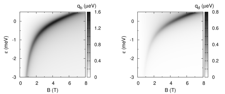
Figure S2 shows the coupling constants and (we consider everywhere the absolute values) as a function of the energy detuning and magnetic field for the AC field amplitude eV and . In both cases the maximum occurs near the anticrossing point which shifts at higher field as the detuning increases. The large negative detuning regime, where the spins are effectively in the Heisenberg limit, is of particular interest in this work when we focus on the transitions between and . In this regime suggesting that singlet-triplet transitions are much faster when the AC field tunes the inter-dot tunnel coupling instead of the energy detuning. Specifically, for meV the transitions can be over an order of magnitude faster. Near zero detuning and are on the same order of magnitude.

In Fig. 2 of the main article the coupling constants and are plotted as a function of the magnetic field for large negative detuning meV. Figure S3 shows and at different detunings for the AC field amplitude eV and . For positive detuning can be equal or greater than . Moreover, for meV at finite magnetic field T. The reason for this particular behaviour is that because and the coefficients in Eq. (2) in the main article have different signs due to the (anti-) bonding character of the states. However, in the large negative detuning regime and assuming that is on the order of then , because either positive or negative terms dominate. In contrast, for any value of the detuning.
IV Transitions between higher eigenstates

In the main article the transitions between the two lowest singlet-triplet eigenstates , are examined. However, the derivation of the two-level Hamiltonian suggests that can describe equally well the transitions between the two eigenstates , by simply considering the appropriate matrix elements which couple to and calculating the coupling constants , . The eigenenergies , are shown in Fig. S1.
We focus on the singlet-triplet eigenstates , and plot in Fig. S4 the ratio as a function of the energy detuning for the AC amplitude eV, and . As in the main article, the magnetic field is taken to be 0.5 T higher than that of the anticrossing point. Following the arguments given in the main article we expect when the component dominates over . This condition is now satisfied for large positive detuning. According to Fig. S4, when the AC field tunes the inter-dot tunnel coupling it results in a significant speedup in the transition rate between the singlet-triplet eigenstates , . This speedup is of the same order of magnitude as that achieved for the eigenstates , examined in the main article (see Fig. 2 lower panel). The basic difference is in the range of the energy detuning. In particular, when the AC field tunes the tunnel coupling the transitions between the singlet-triplet eigenstates , are over an order of magnitude faster for the detuning meV.
References
- (1) K. Ono, G. Giavaras, T. Tanamoto, T. Ohguro, X. Hu, and F. Nori, Phys. Rev. Lett. 119, 156802 (2017).