Virtually the Same:
Comparing Physical and Virtual Testbeds

Abstract

Network designers, planners, and security professionals increasingly rely on large-scale testbeds based on virtualization to emulate networks and make decisions about real-world deployments. However, there has been limited research on how well these virtual testbeds match their physical counterparts. Specifically, does the virtualization that these testbeds depend on actually capture real-world behaviors sufficiently well to support decisions?

As a first step, we perform simple experiments on both physical and virtual testbeds to begin to understand where and how the testbeds differ. We set up a web service on one host and run ApacheBench against this service from a different host, instrumenting each system during these tests.

We define an initial repeatable methodology (algorithm) to quantitatively compare physical and virtual testbeds. Specifically we compare the testbeds at three levels of abstraction: application, operating system (OS) and network. For the application level, we use the ApacheBench results. For OS behavior, we compare patterns of system call orderings using Markov chains. This provides a unique visual representation of the workload and OS behavior in our testbeds. We also drill down into read-system-call behaviors and show how at one level both systems are deterministic and identical, but as we move up in abstractions that consistency declines. Finally, we use packet captures to compare network behaviors and performance. We reconstruct flows and compare per-flow and per-experiment statistics.

From these comparisons, we find that the behavior of the workload in the testbeds is similar but that the underlying processes to support it do vary. The low-level network behavior can vary quite widely in packetization depending on the virtual network driver. While these differences can be important, and knowing about them will help experiment designers, the core application and OS behaviors still represent similar processes.

I Introduction

Network operators and designers rely heavily on testbeds to verify configuration changes, validate new designs, and troubleshoot existing networks without interrupting production services. In some cases, security engineers use testbeds to better understand security incidents, do post-event forensics, and even explore how various countermeasures would perform. Physical testbeds are expensive to build and maintain so virtual testbeds are used as a cost-effective alternative. By running the same OS and software, virtualization offers a higher fidelity than discrete-event simulations. But how do virtualization artifacts affect these testbeds and the experiments they host? How should experimenters account for subtle differences between virtual and physical testbeds?

To date, there has been limited study of the effects of virtualization on virtual testbeds. Instead, we rely on ad hoc assessments of the experiments and results by subject-matter experts to determine whether they make logical sense. We know that virtualization causes higher network latency and lowers throughput [19, 23, 25, 27] for individual virtual machines (VMs). Wang et al. [25] even showed that for small bursts, buffering can cause VMs to receive data at rates that exceed the underlying network.

Our experimental design is informed by our goal: to measure, document, and understand differences between physical and virtual testbeds. We run a representative workload, ApacheBench [1] querying a simple web server. Our experiments vary testbed parameters such as the network driver and workload parameters such as payload size. During these experiments, we measure the systems at three layers of abstraction: application, operating system, and underlying network.

We find notable differences in the system and network-level interactions. For example, when receiving a 1MB payload, all testbeds read a total of 1MB of data. However, they use vastly different numbers of read system calls due to differences in segmentation offloading. Additionally, they transmit differing numbers of packets. These differences in underlying system behaviors are important and have the potential to affect experimental results.

When one considers that computers are fundamentally state machines that cycle through instructions deterministically, one might expect physical and virtual testbeds to have (nearly) identical behaviors. This is particularly true for our workload, which has no inter-request dependencies. One way to model an application’s behavior is through its sequence of system calls. Since our workload consists of many repetitions of the same transaction, we expect the system call traces to contain many repeated sequences. To make the sequences simpler to work with and to normalize the repeated behaviors across sequences of different lengths (caused by different testbeds completing different numbers of transactions), we transform the sequences into Markov Chains as described in Section II. In Section V-D, we show how the Markov chain for the physical and virtual testbeds can create almost identical graph topologies representing system behaviors.

Even though one might expect a deterministic workload, there is variation even when running the same workload on the same physical testbed. So, we must expect some differences between virtual and physical testbeds. Our goal is not to prove whether virtual testbeds are good or bad. It is to understand where and how they differ from physical testbeds so those who use virtual testbeds will be better able to plan their experiments and interpret the results.

II Background

Network simulation tools like NS-2 [15] and OPNET [8] create highly detailed network models to simulate a network’s behavior under many conditions. To ensure simulation reliability, the tools contain simulated versions of all aspects of a network, including endpoints, routers, and switches. These network models follow a set of known behaviors exactly. However, this reliable repetition comes at the cost of decreased accuracy. The simulated network elements model actual components that, in the real world, may display behaviors different from the tool’s built-in components.

Network emulation improves the accuracy of these network models by introducing actual network components. But it is more difficult to scale simulated testbeds to emulate large-scale network environments. Virtualization, utilizing multiple VMs on the same physical machine, permits testbeds to effectively emulate networks containing thousands or even millions of endpoints [20].

Sandia National Laboratories has been researching, developing, and applying large-scale emulations using virtualization as testbeds for over a decade [20]. Sandia has developed several supporting toolsets including minimega [2].

Several other papers have presented testbed orchestration platforms [7, 10, 18, 22]. While our experiments could be run on any of these platforms and most modern hardware, for this paper we focus on the different between physical and virtual on one specific cluster using a single orchestration tool. This allows us to experiment with different parameters within the virtual machine itself (e.g. different network drivers). Future work will expand across different testbed platforms.

Multiple researchers expose differences in latency and throughput in virtualized networking devices [19, 23, 25, 27]. Virtualization can also cause different network behaviors, especially around TCP and congestion control [9, 12, 13]. These papers typically present new approaches for performance improvement. We focus on understanding the differences and how they affect the accuracy of emulations used to understand larger-scale phenomena.

Sequences of system calls can capture the expected behavior of applications in areas such as intrusion detection [11, 14] and filesystem optimization [17]. Previous research [26] used system-call Markov chains for intrusion detection. To the best of our knowledge, this is the first paper to apply such Markov chains to compare virtual to physical testbeds.

A Markov chain is a graph where nodes represent states and edges represent transitions between states. For a sequence of system calls, we empirically create a graph where a node is a system call and two nodes, $X$ and $Y$, are connected by a directed edge (arc) from $X$ to $Y$ i.f.f. the system call $Y$ appears immediately after system call $X$ at least once. Each arc has a weight corresponding to the probability that $Y$ follows $X$. The weight of arc $(X,Y)$ is the percentage of times $Y$ is immediately followed by $X$ in the sequence.

Figure 1 shows a simple Markov chain representing a single user search for an item in a file. The user first tries to open the file. This is the start state, shown with a heavy node boundary. With probability $.01$, there is an error in opening the file, where the new state is “error,” and the process ends. With probability $.99$, the open succeeds and the user code reads the first line. For each line, the user finds what he seeks with probability $.25$. If so, the user closes the file and the search ends. Otherwise, with probability $0.75$ the user continues the search by reading the next line, and the state (current node) does not change.

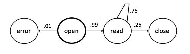
Figure 1: An example of a Markov chain for system calls seen in searching a file line by line.

We can extend this definition to include more of the recent history of system calls by having states represent a set of $N$ consecutive system calls. If a node has an ordered set of calls (label) $c_{1},c_{2},\ldots,c_{N}$, then the next state, represented by neighbors in the graph, has the form $c_{2},c_{3},\ldots,c_{N},c_{\mbox{new}}$, where $c_{\mbox{new}}$ is the next system call seen after $c_{N}$. As $N$ increases, the Markov chain becomes specific to the sequence of system calls that generated it, diminishing the chances of it matching system-call sequences from another process.

We now formalize the “similar/close” concepts we have used so far. We say that two experimentally measured quantities are “close” or “similar” if their means differ by no more than $10$%. This is an arbitrary value for quantitative comparisons in this paper. For a particular application, a subject-matter expert may need to set this comparison point.

We compute $95$% confidence intervals, assuming a standard normal distribution of sample means. Assuming our samples are representative of a random sample of all such experiments, then if we were to repeat the experiment with this size random sample an infinite number of times, the sample mean will be within the confidence interval range $95$% of the time. Overlapping confidence intervals is a stronger definition.

III Methodology

In this section, we detail a methodology to compare workloads across testbeds, whether physical or virtual. Although we consider a single workload in this paper, we ultimately must consider many different network-based workloads using this basic methodology.

The simplest way to compare testbeds is with metrics from the workload itself, such as how much work completes in a fixed amount of time. However, the virtualization overhead almost always leads to physical testbeds outperforming the virtual ones. Therefore, we also take measurements at other levels of abstraction – interactions between the workload and the OS. Specifically, we measure system calls, context switches, and block IO and normalize by work completed to determine the interactions per unit work. This allows direct comparisons between testbeds. Finally, we compare our network-based workload at the network layer. We capture traffic to compare properties of the underlying packets and flows (for TCP-based workloads). These different layers of abstraction allow us to compare behaviors, not just performance.

If there were just one physical and one virtual testbed, our comparison would be fairly straightforward – we would apply the above methodology to both across several workloads and draw our conclusions. Unfortunately, there are many physical and virtual testbeds. These testbeds vary in machine resources (e.g. CPU and memory), network bandwidth (e.g. 100Mbps, 1Gbps), network interface and driver, OSes, etc. To draw broader conclusions about the differences between physical and virtual testbeds, we must perform tests with many parameters to determine if there are any generalizable trends. We do not claim to fully map this space but present an initial mapping that may help us to understand the landscape.

Virtualization allows for multiple VMs on the same machine meaning that virtual testbeds can be many times larger than the underlying physical machines, a practice called oversubscription, which induces contention [20]. As a first step, we assume that our systems are not resource constrained. We believe a strong understanding of normal/non-resource-constrained behavior should come before studying edge cases introduced by oversubscription.

IV Experimental Design

We detail a concrete application of our methodology to a simple HTTP workload. We describe the testbeds, workload, and instrumentation. We repeated each experiment ten times.

IV-A Virtual Testbed Tool: minimega

We use minimega [2] to manage, deploy, and monitor our virtual testbeds. It is the product of over a decade of research and development at Sandia National Laboratories. minimega orchestrates Kernel-based Virtual Machines (KVM [16]) to run unmodified OSes such as Windows, Linux, and Android, that represent real machines in networks of interest. minimega is bundled with other tools to form the open-source minimega toolset, which supports our Emulytics program.

When configuring VMs, the user decides the number of network interfaces, network connectivity, and network drivers. minimega uses 802.1q VLAN tagging via Open vSwitch [4] to support arbitrary network topologies. KVM supports several network drivers with varying properties such as e1000 and virtio. e1000 represents a real e1000 network interface card (NIC) while virtio is a paravirtualized NIC that is implemented specifically for better performance within a VM.

minimega has many other capabilities to support experiments. Its command-and-control layer can execute commands on the VMs and push/pull files. It supports packet captures for individual VMs. It can emulate networks with different speeds based on Linux traffic control, “tc.” For example, minimega can emulate a 1Gbps switch by rate limiting all VMs on a network to 1Gbps. While minimega focuses on virtual testbeds, it can also deploy and run experiments on physical testbeds, as we did for our physical experiments.

We use several other tools in the minimega toolset. protonuke is a simple traffic generator that supports several protocols and acts as either a server or client. vmbetter creates initial ramdisk images that we use for physical hosts and VMs.

IV-B Workload

We use ApacheBench [1], the HTTP server benchmarking tool, to repeatedly load the same page served by protonuke, acting as a simple HTTP server. Client and server run on separate (virtual) machines, connected by a switch. This transaction, an HTTP GET and response, is at the core of almost all of the more complex workloads we test. By keeping to this basic workload we can focus on key system interactions.

We can vary the number of client threads, the number of requests or duration, and HTTP response size. Our experiments use three response sizes: 500B, 1MB and 16MB. We run ApacheBench for 90 seconds, allowing it to complete as many requests as possible (up to 500,000 requests). We use ten client threads, except where noted.

IV-C Virtual Machines

There are many ways to instantiate VMs. We can vary hypervisors, network drivers, CPU pinning, scheduling algorithms, resource allocations, host OS, etc. We focus on the network driver, the glue between the guest OS and the host OS. Specifically, we look at the differences between e1000, which emulates a real e1000 network interface and virtio, which was designed to make VMs more performant. We chose these two drivers because e1000 is the default in minimega (and therefore, often unchanged) and because virtio is the go-to driver to improve networking performance (at least within the Emulytics community). We did not vary the other parameters – we used KVM for the hypervisor, 2GB of memory, and 8 vCPUs. For now, these parameters represent a well-provisioned system able to support the workload.

We base our VMs off an initial ramdisk (initrd) from vmbetter. This allows us to create a minimal install containing few packages and a minimal init program performing only critical functions. Specifically, the init process initializes the filesystem, loads kernel modules, starts sshd, and runs miniccc (the agent with which minimega communicates). This minimizes background-process interference. We do the same for our physical machines.

IV-D Hardware

We ran the physical tests on two identical nodes:

• Dual Intel(R) Xeon(R) E5-2630L 0 @ 2.00GHz

• 24 Cores (6/socket, HT enabled), 125GB Memory

• Interfaces: 1Gbps (igb), 10Gbps (ixgbe)

We ran the VM tests on two identical nodes:

• Dual Intel(R) Xeon(R) E5-2683 v4 @ 2.10GHz

• 64 Cores (16/socket, HT enabled), 503GB Memory

• Interfaces: 100Gbps (mlx5)

These nodes represent our older and newer Emulytics nodes which are well provisioned to run many VMs. The older nodes have both 1Gbps and 10Gbps interfaces, so we can perform tests with both link speeds. The newer nodes have 100Gbps interfaces. For each interface, we list the associated driver.

All physical and virtual machines use the same Linux Kernel version, 4.9.0-4-amd64, the latest available from Debian stretch when we built the images.

IV-E Instrumentation

In Section III, we described the various levels of instrumentation that we use to compare testbeds. Here, we describe the specific instrumentation tools that we use. In Section V-A1, we perform experiments to understand the overhead of instrumentation on the workload.

System Call Traces: We collect system-wide system call traces using sysdig [5]. These traces contain all calls from all programs running on the physical or virtual machine.

Packet Captures (PCAPs): For the physical machines, we capture traffic on the machine itself using tcpdump [6]. For the VMs, we capture traffic from the host using minimega (which uses libpcap) to avoid the performance overhead of capturing within a VM. Since tcpdump also uses libpcap, we do not expect the capture method to introduce any significant differences. We use tcptrace [21] which assembles TCP packets from the PCAPs into flows and computes statistics, such as the number of packets, and retransmits, on a per-flow basis.

Latency: To measure queueing, we use owping [3] to measure the one-way latency between the client and server. We do not synchronize the clocks so we cannot use the absolute latency values. Instead, we use the jitter to infer how much the latency varied over the duration of the experiment.

V Results

In this section, we present our initial results including experimental data and metric comparisons between the physical and virtual testbeds. We analyze the application-level metrics which confirm that the workload behaves as expected, although at different rates. Then, we explore how the underlying interactions with the OS and network vary between the testbeds.

V-A Application-level Metrics

Here we examine the results from ApacheBench for physical, e1000, and virtio drivers for both 1Gpbs and 10Gbps systems. We find an anomaly in e1000 tests but otherwise the results seem quite comparable. We then explore issues with our e1000 results and correlate the anomaly to a known bug.

Size	Physical	e1000	Virtio
500B	14420 $\pm$ 74.3	6476 $\pm$ 707	13590 $\pm$ 139
1MB	112 $\pm$ 0.012	113 $\pm$ 0.12	113 $\pm$ 0.006
16MB	6.97 $\pm$ 0.006	7.05 $\pm$ 0.006	7.09 $\pm$ 0.032

TABLE I: Mean requests per second and confidence intervals for ApacheBench runs for 1Gbps tests.

Table I shows the confidence intervals for mean requests per second for the 1Gbps tests. With the exception of e1000 for small workloads, which we explore later in this section, all systems have similar results. The network driver can have a significant impact on much higher-level application behavior and how well an emulation resembles the physical world. Moreover, the selection of workload size also impacts how representative our results are.

Size	Physical	e1000	Virtio
500B	13080 $\pm$ 101	6734 $\pm$ 867	13631 $\pm$ 139
1MB	638 $\pm$ 2.4	144 $\pm$ 20.6	590 $\pm$ 35.7
16MB	50.0 $\pm$ 0.316	13.2 $\pm$ 0.955	44.5 $\pm$ 2.78

TABLE II: Mean requests per second and confidence intervals for ApacheBench runs for across 10Gbps tests.

Table II shows these same test with an emulated 10Gbps network. Here the differences for e1000 are more pronounced. Once again, we see that the behaviors for physical and virtio are similar. For small payload sizes, virtio actually outperforms the physical system. We speculate and have seen anecdotal evidence that this performance difference may be an artifact of the way our bandwidth-limiting tool emulates a 10Gbps link. At this higher rate, the physical testbed is noticeably more consistent in its behavior than the virtual ones.

V-A1 Instrumentation Overhead

To quantify the overhead of our instrumentation, we ran a set of tests with no instrumentation. Table III shows our ApacheBench results from this test. The most significant impact of our instrumentation is on the physical testbed where there is a 13% drop in performance. We believe this is from the overhead of running tcpdump on the physical testbed. In the virtual testbeds, virtio drops by 5% while e1000 improves. We suspect the latter is due to high variability in the e1000 performance.

Size	Physical	e1000	Virtio
1Gbps
500B	16459 $\pm$ 57	5740 $\pm$ 559	14373 $\pm$ 182.8
16MB	6.98 $\pm$ 0.0062	7.05 $\pm$ 0.0062	7.09 $\pm$ 0.012
10Gbps
500B	15013 $\pm$ 104	5474 $\pm$ 374	14431 $\pm$ 227
16MB	60.1 $\pm$ 0.39	11.7 $\pm$ 1.61	42 $\pm$ 1.74

TABLE III: Mean request per second and confidence intervals for ApacheBench runs without instrumentation.

V-A2 Exploring the Outlier, e1000

To understand why our e1000 testbed behaves so differently, we turned to the PCAPs that we collect. We observed that numerous experiments had an errant behavior that would delay connections for some multiple of 13 seconds. Upon a more detailed examination, we saw that data had been sent and acknowledged but the server was still behaving as if it had not been acknowledged (for all connections). Then, after a multiple of 13 seconds the server returned to normal behavior. From the kernel logs for the VM, we found that the kernel reset the network adapter multiple times after detecting a transmit queue timeout. Network adapter resets are commonly observed behavior when a bug in the underlying NIC driver is encountered. We plan to discard experiments that trigger this bug in the future.

V-B OS-Level Metrics

We now investigate differences in how ApacheBench interacts with the OS as it makes requests. We focus on data read and read system calls as these are a key parts of the workload. System calls present a middle ground in abstraction between the request per second and the bytes per request. We normalize using the number of completed requests, to compare across testbeds completing vastly different numbers of requests.

We look at a low-level metric that should be strongly consistent: bytes sent per request completed. Figure 2(a) plots the number of bytes sent by the server per request completed, including retransmits. While it may seem trivial to show that these numbers are consistent, this measure is independent of timing and network rates so it provides a basic ability to show that the underlying process is consistent and deterministic. This plot shows a clearly consistent behavior from all testbeds.

Our underlying thesis for Emulytics is that since we run the same software, we should get the same behavior. Since a thread is a deterministic machine that works through the same lock steps in the same way for the same input, we expect somewhere in our experiments to see this high level of consistency across all tests.

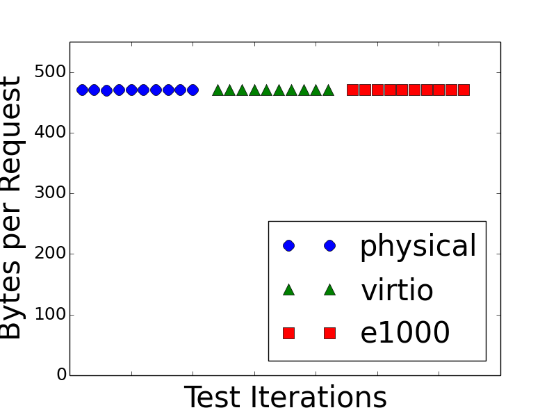
(a) Bytes per Request

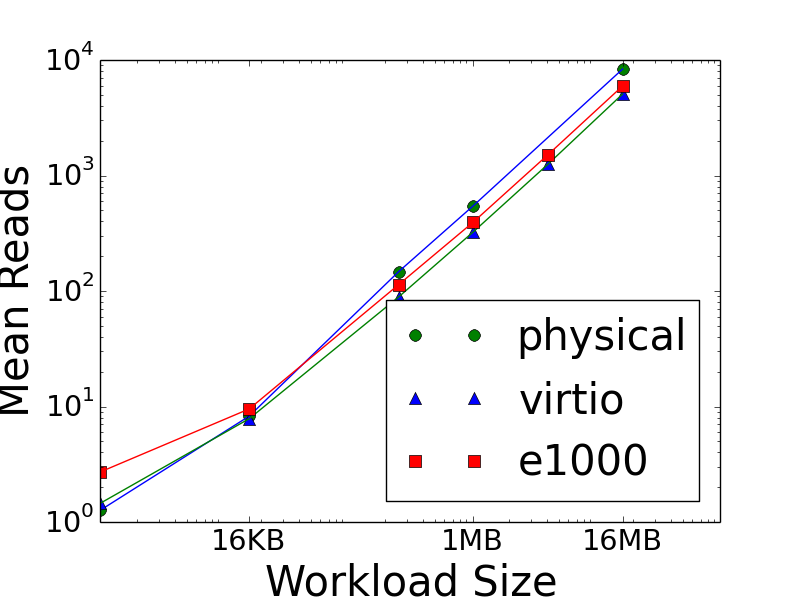
(b) Mean read calls

Figure 2: (a) Bytes per Request for 500B workloads over 1Gpbs network. (b) Mean number of read system calls needed to complete a request across varying workload sizes.

At a higher level of abstraction, but still within the OS layer, we consider number of reads per request. Table IV shows the mean number of reads per request for the 1Gbps test. As expected, the number of reads increases as the payload grows. In all but the small payload workload, the physical testbed performs more reads than the virtual ones. In all cases, virtio requires fewer reads than e1000.

Size	Physical	e1000	Virtio
500B	1.34	2.95	1.75
1MB	547.44	395.02	325.27
16MB	8345.82	5954.81	5072.02

TABLE IV: Mean number of read system calls per request for 1Gbps test.

Table V shows the mean number of reads per request for the 10Gbps test. Unlike in Table IV, the physical testbed has fewer reads per request than the virtual testbeds in all but one case. This could be a result of the physical driver being different for the 1Gbps and 10Gbps test which use igb and ixgbe, respectively.

Size	Physical	e1000	Virtio
500B	1.72	3.02	1.69
1MB	260.15	341.84	275.80
16MB	4098.74	4687.41	4102.61

TABLE V: Mean number of read system calls per request for 10Gbps test.

Finally, we look more broadly at the number of read system calls across a wider range of workload sizes. Figure 2(b) shows the mean number of read calls normalized over the mean requests per second from ApacheBench. Here we begin to see the behavior of each process start to diverge.

V-C Network-Level Metrics

From the traffic captures, we can gain a better understanding of how packets generated by the various workloads propagate through the testbeds. Table VI shows the mean packets per request for 1Gbps tests. As before, we see physical and virtio have similar behaviors, though other than for the smallest response size, not quite at our $10$% similarity threshold. Again, e1000 stands out as different.

Size	Physical	e1000	Virtio
500B	5.00 $\pm$ 0.08	5.00 $\pm$ 0.10	5.00 $\pm$ 0.12
1MB	67.7 $\pm$ 2.19	105.7 $\pm$ 9.04	77.3 $\pm$ 10.2
16MB	834 $\pm$ 46.3	1527 $\pm$ 817.40	1087 $\pm$ 706

TABLE VI: Mean number of packets per request for 1Gbps test and standard deviation.

Next, we used owamp data to measure the network jitter. This metric offers insights into the network queuing behavior. If the network stack is filled with many packets the jitter will indicate increased delays as the one-way latency traffic queues while waiting for transmission over network links. Table VII shows how our jitter varied across our 1Gbps tests. Here we see that e1000, with the exception of the 16MB workload, more closely matches the end-to-end jitter characteristics seen in the physical testbed. The virtio testbed provides consistently lower jitter which, while theoretically beneficial, could mask problems that would occur in the real world if a given workload was heavily influenced by jitter.

Size	Physical	e1000	Virtio
500B	0.26 $\pm$ 0.03	0.25 $\pm$ 0.074	0.10 $\pm$ 0.00
1MB	0.29 $\pm$ 0.019	0.24 $\pm$ 0.03	0.16 $\pm$ 0.03
16MB	0.28 $\pm$ 0.025	0.34 $\pm$ 0.043	0.16 $\pm$ 0.03

TABLE VII: Mean jitter measured across the network (in milliseconds) with confidence intervals for 1Gbps.

V-D System-Call Markov Chains

We propose to use two analyses from the system-call traces to determine whether the application behavior on the virtual testbeds are “close enough” to the physical testbed. We examine a specific set of parameters for simplicity: single thread, 1Gbps network, and 500B response. These analyses will need to be repeated for every set of parameters to make broader comparisons between the testbeds.

Figure 3 shows pruned examples of these Markov chains for ApacheBench across the testbeds. We combined 10 runs of each, dropped edges with weight less then $.001$ and renormalized the probabilities around each node. Client Markov chains had identical topology and nearly identical weights. Server Markov chains disagreed on edge existence by up to 22% and had more weight variation on similar edges.

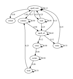
Figure 3: Client Markov chain for physical, e1000, and virtio. We dropped edges of weight less than $.001$ and renormalized.

We can walk a Markov chain using the sequence of system calls from a run on a virtual or physical testbed to compute the probability the Markov chain would generate that sequence. We show the walk/computation process with the Markov chain from Figure 1 and the sequence (open, read, read, read). We start at the node labeled “open.” The next element is the first “read,” There is an edge from the “open” node to the “read” node with weight $.99$, so the first pair of system calls (open, read) occurs with probability $.99$. Similarly, there is an edge from the current node (“read”) to a node with the next element of the sequence (the second read). This has probability $.75$. In Markov chains, each transition is independent, so the probability of seeing the first part of the sequence (open, read, read) is $.99\times.75$. The next step is the same. So the probability of the sequence (open, read, read, read) is $.99\times(.75)^{2}$. The probability for the sequence (open, read, read, close) is $.99\times.75\times.25$, since the last transition goes from the “read” node to the “close” node, which happens with probability $.25$ Because each additional sequence element (system call) multiplies the final probability by a number less than 1, the total can become quite small and sequence length becomes important for comparison. For example, for the Markov chain in Figure 1, the most probable sequence of length 17 is open followed by 16 reads. This sequence has lower probability than the sequence (open, error). Thus, we will compare sequences of equal lengths, where the relative sizes of the probabilities are a valid means of comparison, even though the absolute probability for long sequences are tiny.

More formally, given a sequence of system calls and a Markov chain with system-call node labels, we start at the Markov-chain node that matches the first element of the sequence. Moving to the next element in the sequence (system call $s_{i}$) is a transition in the Markov chain to the node with the label $s_{i}$. We continue the walk to the end of the sequence. The final probability is the product of the weights of every edge we traverse with multiplicities.

We built Markov chains using runs in the physical testbed by creating a node for every system call in the sequence and an edge for each pair of consecutive calls. Edge $(c_{i},c_{j})$ is weighted by the percentage of times the call $c_{i}$ is followed by $c_{j}$. We then compared the relative probabilities when walking the chain using a sequence from e1000 to that from virtio. For a baseline, we also include the probability from walking the Markov chain with the physical sequence. Since we ran ten iterations of each physical, e1000, and virtio, we build ten Markov chains for each of the physical tests and compare to each of the ten sequences of each type.

Consider a Markov chain created by sequence A. When walking that chain using a sequence B, is it possible that there is no edge for a particular transition $(c_{i},c_{j})$. That sequence did not appear in sequence A. We call this an invalid transition, which gives the walk probability zero.

We apply this technique to the system-call sequences from ApacheBench with a single thread. Table VIII shows how many times an invalid transition occurs. We found that the invalid transitions typically occur in the initialization phase of the workload so we also report the number of invalid transitions when we skip the first 1 million (1M) system calls.

Sequence	No Skip	Skip 1M
physical	32	0
e1000	26	0
virtio	26	0

TABLE VIII: Invalid transitions from 100 walks of Markov chains using sequences from physical, e1000, and virtio.

Table IX shows the average probability when walking a Markov chain built from the physical testbed with e1000 and virtio sequences relative to the average when walking the same chain with physical sequences (i.e. $P(\mbox{e1000})/P(\mbox{physical})$. We limit the sequences to 2M system calls to ensure that we compare sequences of the same length (the shortest sequence is just over 3M system calls). As before, we also report on the probabilities when we skip the first 1M system calls.

Sequence	No Skip	Skip 1M
e1000	E+5531	E+5402
virtio	E-33288	E-28214

TABLE IX: Relative probabilities from walking Markov chains built from physical testbed using sequences from e1000 and virtio to physical. We omit the bases as they are irrelevant given the magnitudes of the exponents.

This chart shows that the e1000 sequences are many orders of magnitude more probable than the physical sequences while the virtio sequences are many orders less. We suspect that this is because we built the Markov chains with $N=1$ which does not include any system-call history. We performed some initial experiments with $N=2$ and found that the physical sequences become more likely, on average, than the e1000 sequences. We do not report on those results further because the number of invalid transitions increases significantly so that we have very few probabilities to average.

VI Conclusion

We have defined a first repeatable method to quantitatively compare physical and virtual testbeds. We have applied these methods to simple network tests to show our method’s utility. Our experiments show that, for our simple workload, our virtual testbed behaves reasonably close to its physical counterpart, within our $10$% threshold in many cases. We make this assessment using multiple levels of abstraction from workload metrics to system interactions to packet captures.

We hope this paper will encourage discussion and that other researchers will extend these comparison methods for these simple tests and for more complex tests.

Acknowledgements We thank Rob Johnson (VMWare), Ben Reed (San Jose State University), and Jeff Boote (Netflix) for helpful discussions and detailed comments on an early draft. Sandia National Laboratories is a multimission laboratory managed and operated by National Technology and Engineering Solutions of Sandia, LLC., a wholly owned subsidiary of Honeywell International, Inc., for the U.S. Department of Energy’s National Nuclear Security Administration under contract DE-NA-0003525.

References

- [1] ab – apache http server benchmarking tool. https://httpd.apache.org/docs/2.4/programs/ab.html.
- [2] minimega: a distributed vm management tool. http://minimega.org/.
- [3] One-way ping (owamp). http://software.internet2.edu/owamp/.
- [4] Open vswitch. http://www.openvswitch.org/.
- [5] sysdig. https://sysdig.com/.
- [6] tcpdump & libpcap. http://www.tcpdump.org/.
- [7] Benzel, T. The science of cyber security experimentation: the deter project. In Proceedings of the 27th Annual Computer Security Applications Conference (2011), ACM, pp. 137–148.
- [8] Chang, X. Network simulations with opnet. In Proceedings of the 31st conference on Winter simulation: Simulation—a bridge to the future-Volume 1 (1999), ACM, pp. 307–314.
- [9] Cheng, L., Lau, F. C. M., Cheng, L., and Lau, F. C. M. Revisiting TCP congestion control in a virtual cluster environment. IEEE/ACM Transactions on Networking 24, 4 (Aug. 2016).
- [10] Chun, B., Culler, D., Roscoe, T., Bavier, A., Peterson, L., Wawrzoniak, M., and Bowman, M. Planetlab: An overlay testbed for broad-coverage services. SIGCOMM Comput. Commun. Rev. 33, 3 (July 2003).
- [11] Forrest, S., Hofmeyr, S. A., Somayaji, A., and Longstaff, T. A. A sense of self for unix processes. In Proceedings 1996 IEEE Symposium on Security and Privacy (May 1996), pp. 120–128.
- [12] Gamage, S., Kompella, R. R., Xu, D., and Kangarlou, A. Protocol responsibility offloading to improve TCP throughput in virtualized environments. ACM Transactions on Computer Systems 31, 3 (2013).
- [13] He, K., Rozner, E., Agarwal, K., Gu, Y. J., Felter, W., Carter, J., and Akella, A. AC/DC TCP: Virtual congestion control enforcement for datacenter networks. In Proceedings of the 2016 ACM SIGCOMM Conference, SIGCOMM ’16.
- [14] Hofmeyr, S. A., Forrest, S., and Somayaji, A. Intrusion detection using sequences of system calls. Journal of computer security 6, 3 (1998), 151–180.
- [15] Issariyakul, T., and Hossain, E. Introduction to network simulator NS2. Springer Science & Business Media, 2011.
- [16] Kivity, A., Kamay, Y., Laor, D., Lublin, U., and Liguori, A. kvm: the linux virtual machine monitor. In Proceedings of the Linux symposium (2007), vol. 1, Dttawa, Dntorio, Canada, pp. 225–230.
- [17] Kroeger, T. M., and Long, D. D. The case for efficient file access pattern modeling. In Proceedings of the Seventh Workshop onHot Topics in Operating Systems, 1999. (1999), IEEE, pp. 14–19.
- [18] Lantz, B., Heller, B., and McKeown, N. A network in a laptop: rapid prototyping for software-defined networks. In Proceedings of the 9th ACM SIGCOMM Workshop on Hot Topics in Networks (2010), ACM, p. 19.
- [19] Menon, A., Santos, J. R., Turner, Y., Janakiraman, G. J., and Zwaenepoel, W. Diagnosing performance overheads in the xen virtual machine environment. In Proceedings of the 1st ACM/USENIX international conference on Virtual execution environments (2005), ACM, pp. 13–23.
- [20] Minnich, R., and Rudish, D. Ten million and one penguins, or, lessons learned from booting millions of virtual machines on hpc systems. In Proc. Workshop on System-level Virtualization for High Performance Computing in conjunction with EuroSys (2010), vol. 10.
- [21] Ostermann, S. tcptrace. http://www.tcptrace.org/.
- [22] Ricci, R., Eide, E., and Team, C. Introducing CloudLab: Scientific infrastructure for advancing cloud architectures and applications. ; login:: the magazine of USENIX & SAGE 39, 6 (2014), 36–38.
- [23] Rizzo, L., Lettieri, G., and Maffione, V. Speeding up packet i/o in virtual machines. In Proceedings of the ninth ACM/IEEE symposium on Architectures for networking and communications systems (2013), IEEE Press, pp. 47–58.
- [24] Tange, O. Gnu parallel - the command-line power tool. ;login: The USENIX Magazine 36, 1 (Feb 2011), 42–47.
- [25] Wang, G., and Ng, T. E. The impact of virtualization on network performance of amazon ec2 data center. In INFOCOM, 2010 Proceedings IEEE (2010), IEEE, pp. 1–9.
- [26] Warrender, C., Forrest, S., and Pearlmutter, B. Detecting intrusions using system calls: alternative data models. In Proceedings of the 1999 IEEE Symposium on Security and Privacy (Cat. No.99CB36344) (1999), pp. 133–145.
- [27] Whiteaker, J., Schneider, F., and Teixeira, R. Explaining packet delays under virtualization. ACM SIGCOMM Computer Communication Review 41, 1 (2011), 38–44.