A Morphological Classification Model to Identify Unresolved PanSTARRS1 Sources:
Application in the ZTF Real-Time Pipeline

Abstract

In the era of large photometric surveys, the importance of automated and accurate classification is rapidly increasing. Specifically, the separation of resolved and unresolved sources in astronomical imaging is a critical initial step for a wide array of studies, ranging from Galactic science to large scale structure and cosmology. Here, we present our method to construct a large, deep catalog of point sources utilizing Pan-STARRS1 (PS1) 3$\pi$ survey data, which consists of $\sim$3$\times 10^{9}$ sources with $m\lesssim 23.5$ mag. We develop a supervised machine-learning methodology, using the random forest (RF) algorithm, to construct the PS1 morphology model. We train the model using $\sim$5$\times 10^{4}$ PS1 sources with HST COSMOS morphological classifications and assess its performance using $\sim$4$\times 10^{6}$ sources with Sloan Digital Sky Survey (SDSS) spectra and $\sim$2$\times 10^{8}$ Gaia sources. We construct 11 “white flux” features, which combine PS1 flux and shape measurements across 5 filters, to increase the signal-to-noise ratio relative to any individual filter. The RF model is compared to 3 alternative models, including the SDSS and PS1 photometric classification models, and we find that the RF model performs best. By number the PS1 catalog is dominated by faint sources ($m\gtrsim 21$ mag), and in this regime the RF model significantly outperforms the SDSS and PS1 models. For time-domain surveys, identifying unresolved sources is crucial for inferring the Galactic or extragalactic origin of new transients. We have classified $\sim$1.5$\times 10^{9}$ sources using the RF model, and these results are used within the Zwicky Transient Facility real-time pipeline to automatically reject stellar sources from the extragalactic alert stream.

1 Introduction

The proliferation of wide-field optical detectors has led to a plethora of imaging catalogs in the past two decades. Separating unresolved point sources (i.e., stars and quasi-stellar objects [QSOs]) from photometrically extended sources (i.e., galaxies) is one of the most challenging and important steps in the extraction of astronomical information from these imaging catalogs. For faint sources especially, performing this task well accelerates our progress in understanding the Universe (e.g., Sevilla-Noarbe et al. 2018). Separating resolved and unresolved sources allows us to investigate the nature of dark matter by: (i) tracing structure in the Milky Way halo (e.g., Belokurov et al. 2006), (ii) measuring galaxy-galaxy correlation functions (e.g., Ross et al. 2011; Ho et al. 2015), and (iii) detecting the weak lensing signal from cosmic shear (Soumagnac et al., 2015). Complete, and pure, catalogs of galaxies can be used to assess the the geometry of the Universe (Yasuda et al., 2001) and the theory of galaxy formation (e.g., Loveday et al. 2012; Moorman et al. 2015). Finally, for time-domain surveys, point-source catalogs enable an immediate classification for all newly discovered variable phenomena as being either Galatic or extragalactic in origin (e.g., Berger et al. 2012; Miller et al. 2017).

Given the many applications for separating point sources from galaxies, we turn our attention to the Pan-STARRS1 (PS1) 3$\pi$ survey (Chambers et al., 2016), whose $\sim$3$\times 10^{9}$ source catalog provides a felicitous data set.

The 1.8 m PS1 telescope is equipped with a wide-field ($\sim$7 deg²) 1.4 gigapixel camera and is located at Haleakala Observatory in Hawaii (Hodapp et al., 2004). PS1 primarily uses five broadband filters, $g_{\mathrm{P1}}$, $r_{\mathrm{P1}}$, $i_{\mathrm{P1}}$, $z_{\mathrm{P1}}$, and $y_{\mathrm{P1}}$ (hereafter $grizy_{\mathrm{P1}}$). The PS1 3$\pi$ survey scanned the entire visible sky ($\delta>-30^{\circ}$) $\sim$60 times in the five filters over a 4 yr time span (Chambers et al., 2016). This repeated imaging was used to create deep stacks (Magnier et al., 2016a), with a typical 5$\sigma$ depth of $\sim$23.2 mag and a median seeing of $1.19\arcsec$ in the $r$-band (Tonry et al., 2012; Schlafly et al., 2012; Chambers et al., 2016). The first PS1 data release (DR1) provides flux and pixel-based shape measurements for $>$3 billion sources (Flewelling et al., 2016).

Our aim is to develop a large, deep catalog of resolved and unresolved sources using PS1 data. The catalog is general purpose and can serve many different science goals, however, our immediate goal is to support the real-time search for transients in the Zwicky Transient Facility (ZTF; Bellm et al. 2018). Previously, a similar catalog was developed using Palomar Transient Factory (PTF) data (Miller et al., 2017).

The PTF point-source catalog was developed using SExtractor (Bertin & Arnouts, 1996) flux and shape measurements made on deep stacks of PTF images. Stars and galaxies were separated using a machine learning methodology built on the random forest (RF) algorithm (Breiman, 2001). Briefly, supervised machine learning methods build a non-parametric mapping between features, measured properties, and labels, the target classification, via a training set. The training set contains sources for which the labels are already known, facilitating the construction of a features to labels mapping. Following this training, the machine learning model can produce predictions on new observations where the labels are unknown.

The PTF point-source catalog was constructed to support the real-time search for electromagetic counterparts to gravitational wave events. Given that these events are expected to be very rare (e.g., Scolnic et al. 2018), the figure of merit (FoM) for the PTF model was defined as the true positive rate (corresponding to the fraction of point sources that are correctly classified) at a fixed false positive rate (fraction of resolved sources that are misclassified) equal to 0.005 (Miller et al., 2017). Maximizing the FoM will reject as many point sources as possible, while still ensuring that nearly every extragalactic transient ($\sim$99.5%) remains in the candidate stream. While the PTF point-source catalog includes $\sim$1.7$\times 10^{8}$ objects, the PS1 database includes an order of magnitude more sources.

A resolved–unresolved separation model built on PS1 data will produce dramatic improvements over the PTF catalog. PS1 observations are deeper, feature better seeing, and include 5 filters (the PTF catalog was built with observations in a single filter, $R_{\mathrm{PTF}}$). Additionally, one of the 12 CCDs in the PTF camera did not work (Law et al., 2009), meaning $\sim$8% of the $\delta>-30^{\circ}$ sky has no PTF classifications.

Here, we construct a new morphological classification model using PS1 DR1 data in conjunction with a new machine learning methodology. The model is trained using Hubble Space Telescope observations, which should provide an improvement over the Sloan Digital Sky Survey (SDSS; York et al. 2000) spectroscopic training set used in Miller et al. (2017). As in Miller et al. (2017), we use the RF algorithm to separate point sources and extended sources and we optimize our model to maximize the same FoM. Our new PS1 model outperforms alternatives and has already been incorporated into the ZTF real-time pipeline.

Alongside this paper, we have released our open-source analysis, and queries to recreate the data utilized in this study. These are available online at https://github.com/adamamiller/PS1_star_galaxy. The final ZTF–PS1 catalog created during this study is available as a High Level Science Product via the Mikulski Archive for Space Telescopes (MAST) at http://dx.doi.org/10.17909/t9-xjrf-7g34 (catalog doi:10.17909/t9-xjrf-7g34).

2 Model Data

Data for the resolved–unresolved model were obtained from the PS1 casjobs server. The PS1 database provides flux measurements via aperture photometry, point-spread-function (PSF) photometry, and Kron (1980) photometry. These flux measurements are produced by PS1 in 3 different ways. The mean brightness measured on the individual PS1 frames is reported in the MeanObject table, the mean brightness measured via forced-PSF/aperture photometry on the individual PS1 frames is reported in the ForcedMeanObject table, and finally, the brightness measured on the full-depth stacked PS1 images is reported in the StackObjectThin table. The StackObjectAttributes table further supplements these tables with point-source object shape measurements, which prove useful for identifying unresolved sources. Ultimately, see §4.2, we use flux measurements from the StackObjectThin table and shape measurements from the StackObjectAttributes table to build our models.

2.1 The HST Training Set

A fundamental challenge in the construction of any supervised machine learning model is the curation of a high-fidelity training set. A subset of the data that requires classification must have known labels so the machine can learn the proper mapping between features and labels. The superior image quality of the Hubble Space Telescope (HST) provides exceptionally accurate morphological classifications, making it an ideal source of a training set for lower quality ground-based imaging (e.g., Lupton et al. 2001). The downside of HST is that the field of view is relatively small, so it is difficult to construct a large and diverse training set suitable for predictions over the entire sky.

We use the largest contiguous area imaged by HST, the 1.64 deg² COSMOS field, to construct a training set for our models. Morphological classifications of HST COSMOS sources are provided in Leauthaud et al. (2007). Leauthaud et al. demonstrate reliable classifications to $\sim$25 mag, which is significantly deeper than the faintest sources detected by PS1. We identify counterparts in the PS1 and HST data by performing a spatial crossmatch between the two catalogs using a 1″ radius. We further excluded sources from the Leauthaud et al. (2007) catalog with $\texttt{MAG\_AUTO}>25$ mag, as these sources are too faint to be detected by PS1, meaning their crossmatch counterparts are likely spurious. Following this procedure, we find that there are 87,431 sources in the Leauthaud et al. (2007) catalog with PS1 counterparts. Of these, 80,974 are unique in that there is a one-to-one correspondence between HST source and a single PS1 ObjID. The training set is further reduced to 75,927 once our detection criteria are applied (see §4.2), and, of those, only 47,093 have $\texttt{nDetections}\geq 1$ in the PS1 database (hereafter, the HST training set).

2.2 The SDSS Training Set

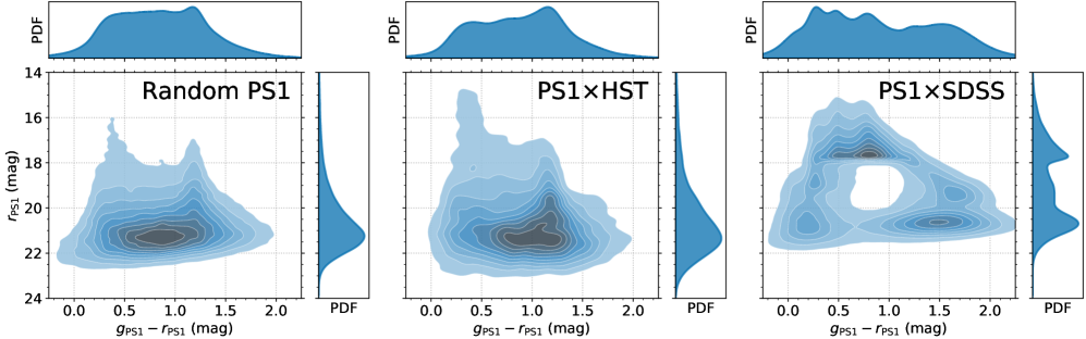
Figure 1: PS1 color-magnitude diagrams for left: $10^{6}$ randomly selected PS1 sources, center: the HST training set, and right: the SDSS training set. The primary panels show a two-dimensional (2D) Gaussian kernel density estimate (KDE) of the probability density function (PDF) of each subset of sources in the $r_{\mathrm{PS1}}$ vs. $g_{\mathrm{PS1}}-r_{\mathrm{PS1}}$ plane. The shown contour levels extend from 0.9 to 0.1 in 0.1 intervals. To the top and right of the primary panels are marginalized 1D KDEs of the PDF for the $g_{\mathrm{PS1}}-r_{\mathrm{PS1}}$ color and $r_{\mathrm{PS1}}$ brightness, respectively. Kron aperture measurements from the StackObjectThin table are used to estimate each of the PDFs.

The SDSS spectroscopic catalog classifies everything it observes as either a star, galaxy, or quasi-stellar object (QSO). Using a $1\arcsec$ cross-match radius, we find 3,834,627 sources with SDSS optical spectra have PS1 counterparts (hereafter, the SDSS training set). Thus, with an orders of magnitude larger training set, and spectroscopic classifications that should be both pristine and superior to mophological clsasifications, one might expect the SDSS training set to be optimal for training the machine learning model. However, as noted in Miller et al. (2017), the SDSS spectroscopic targeting algorithms were highly biased, and as a result these sources prove challenging as a training set.

Color-magnitude diagrams (CMDs) of the HST and SDSS training sets are compared to a random selection of $10^{6}$ sources from the PS1 database in Figure 1. It is clear from Figure 1 that the SDSS training set is completely different from typical sources in PS1 and that there are few SDSS sources in the highest density regions of the PS1 CMD. Given the stark mismatch between typical PS1 sources and the SDSS training set, we adopt the HST training set for the development of our model. We retain the SDSS training set as an independent test set to assess the accuracy of the model following construction.

3 Model Features

In addition to developing a training set, we must select features to use as an input for the model. As noted in §2, the PS1 database provides flux and shape measurements in each of the $grizy_{\mathrm{PS1}}$ filters. Adopting each of these measurements as features for the model presents a significant problem: missing data. There are relatively few sources in the PS1 database that are detected in all 5 filters. Typically, to cope with missing data one can either (i) remove sources detected in fewer than 5 filters, or (ii) assign some value, via either imputation (e.g., Miller et al. 2017) or the use of a dummy variable, to the missing data. Given that the vast majority of PS1 sources are faint and are not detected in all 5 filters, neither of these possiblities is attractive for our present purposes.

Rather than use the raw features from the database, we engineer a series of “white flux” features that combine the relevant measurements across all filters in which a source is detected. In a given filter, a source is detected if the $\mathtt{PSFFlux}_{f}$, $\mathtt{KronFlux}_{f}$, and $\mathtt{ApFlux}_{f}$ are all $>0$, where the $f$ subscript refers to a specific filter. The “white flux” feature is then created as:

$$\mathtt{white[Feat]}=\frac{\sum_{f}^{f=grizy_{\mathrm{PS1}}}w_{f}\,\mathtt{Feat}_{f}\,\mathrm{det}_{f}}{\sum_{f}^{f=grizy_{\mathrm{PS1}}}w_{f}},$$ (1)

where the sum is over the 5 PS1 filters, Feat is the feature from the StackObjectAttributes table, $\mathrm{det}_{f}=1$ if the source is detected in the $f$ filter, as defined above, or $\mathrm{det}_{f}=0$ if not detected, and $w_{f}$ is the weight assigned to each filter:

$$w_{f}=\left(\frac{\mathtt{KronFlux}_{f}}{\mathtt{KronFluxErr}_{f}}\right)^{2},$$ (2)

equivalent to signal-to-noise ratio (SNR) squared in the given filter. Ultimately, the “white flux” features correspond to a weighted mean, with weights equal to the square of the SNR (Bevington & Robinson, 2003).

Our final model includes 11 “white flux” features to separate resolved and unresolved sources. The database features include: PSFFlux, KronFlux, ApFlux, ExtNSigma, KronRad, psfChiSq, psfLikelihood, momentYY, momentXY, momentXX, and momentRH. The remaining features in the database were either uninformative or would bias the model, such as R.A. and Dec. (see e.g., Richards et al. 2012). We do not directly include whitePSFFlux, whiteKronFlux, and whiteApFlux in the model. We found that the inclusion of these features resulted in a bias whereby all sources brighter than $\sim$16 mag were automatically classified as point sources. Instead, we include the ratio of the different flux measures: whitePSFKronRatio = whitePSFFlux/whiteKronFlux, whitePSFApRatio = whitePSFFlux/whiteApFlux, as well as a third feature whitePSFKronDist (see §4.2).

As we previously alluded to, the primary benefit of the “white flux” features is that they can be calculated for every source in PS1 thus allowing each to be compared on common ground. Furthermore, the SNR for the “white flux” features is greater than the SNR for the equivalent feature in a single filter. The downside of these features is that for some sources, especially at the bright end, color information is lost. While a blue source and red source with identical whitePSFFlux values are intrinsically very different, the “white flux” features obscure that information for the classifier. Ultimately, we tested models using the “white flux” features with and without additional color features and found that they are statistically equivalent when tested with the HST training set.

The direct use of color information as model features would require reddening corrections for all PS1 sources. Not only is this a daunting task, but accurate corrections would require a priori knowledge as to which sources are Galactic and which are extragalactic (e.g., Green et al. 2015). The PS1 catalog is being developed precisely to answer this question. Furthermore, the pencil beam sample from the HST training set traces a narrow range of dust columns, so the application of a model including color information without reddening corrections would lead to biased classifications (Sevilla-Noarbe et al., 2018), particularly in regions of high reddening (e.g., the Galactic plane). We conclude that the benefits of the “white flux” features, which eliminate the need for reddening corrections, outweigh any losses from the exclusion of color information.

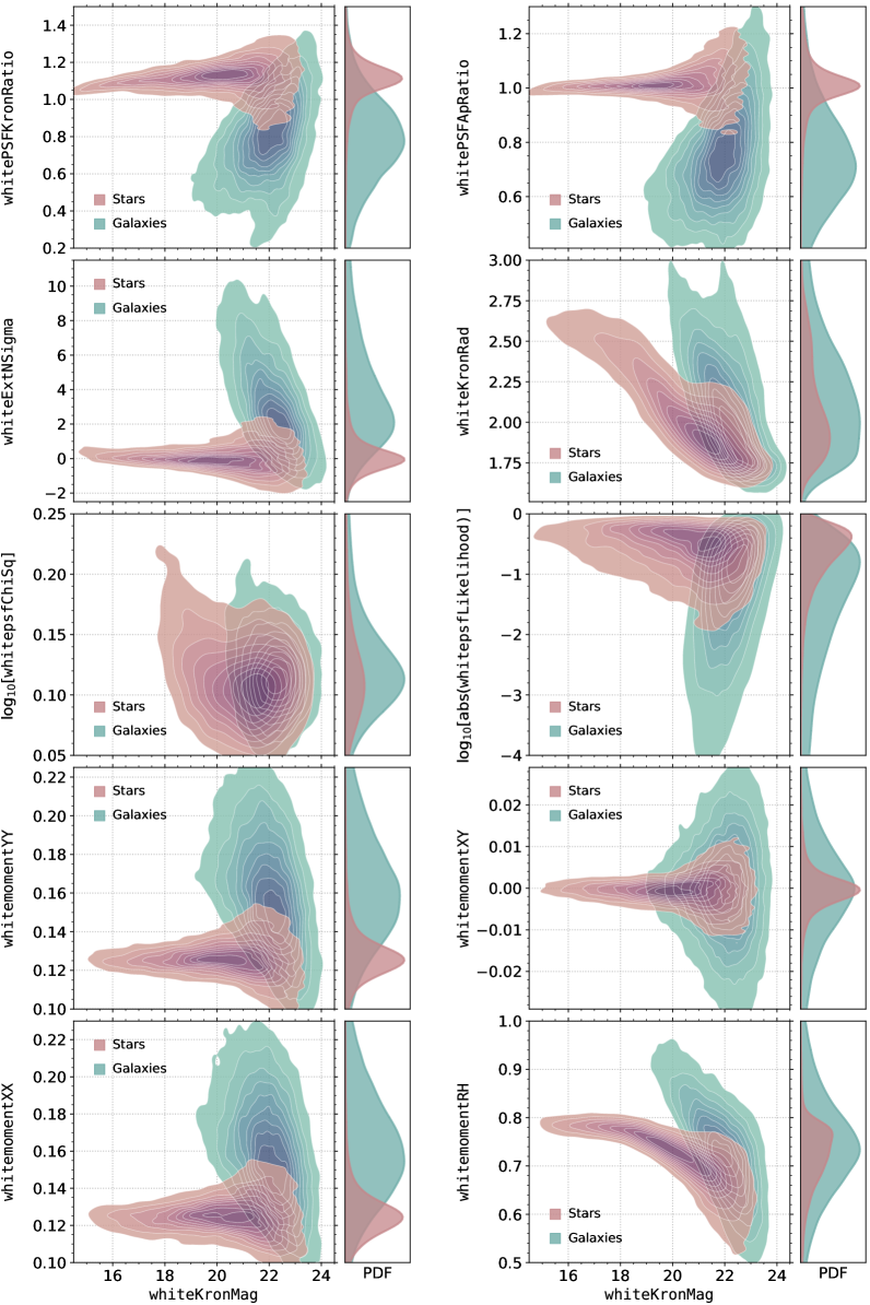
Figure 2: The primary square panels show Gaussian KDEs of the PDF for each of the “white flux” features as a function of whiteKronMag ($=-2.5\log_{10}[\mathtt{whiteKronFlux}/3631]$) for all sources in the HST training set. Unresolved point sources (labeled stars) are shown via the red-purple contours, while resolved, extended objects (labeled galaxies) are shown via blue-green contours. The shown contour levels extend from 0.9 to 0.1 in 0.1 intervals. To the right of each primary panel is a marginalized 1D KDE of the PDF for the individual features, where the amplitudes of the KDEs have been normalized by the relative number of point sources and extended objects. The clear overlap between faint resolved and unresolved sources suggests that a machine learning model may provide significant improvement over the PS1 and simple models.

The distribution of “white flux” features for point sources and extended objects in the HST training set is shown in Figure 2 (whitePSFKronDist is shown in Figure 3). As might be expected, it is clear from Figure 2 that point sources and extended objects are easily separated at the bright end ($\lesssim 20$ mag), but there is significant overlap in the featurespace between the two populations at the faint end ($\sim$23 mag). Machine learning algorithms are capable of capturing non-linear behavior in multidimentional data sets, which will prove especially useful for the sources under consideration in the PS1 data set.

4 Model Construction

4.1 The PS1 Baseline Model

To establish a baseline for the performance of our resolved–unresolved separation models we adopt the classification criteria in the PS1 documentation, namely sources with

$$\mathtt{iPSFMag}-\mathtt{iKronMag}>0.05\;\mathrm{mag},$$

are classified as galaxies. The documentation notes that this classification can be performed using photometry from any of the MeanObject, ForcedMeanObject, or StackObjectThin tables. The PS1 documentation further notes that this basic cut does not perform well for sources with $i\gtrsim 21\,\mathrm{mag}$, which constitutes the majority of sources detected by PS1, and motivates us to develop alternative models. We use the performance of the $\mathtt{iPSFMag}-\mathtt{iKronMag}>0.05\;\mathrm{mag}$ model (hereafter, the PS1 model) as a baseline to compare to the models discussed below.

4.2 Simple Model

While our ultimate goal is to build a machine learning model to identify point sources (§4.3), we first construct a straightforward model. This model is inspired by the SDSS photo pipeline (Lupton et al., 2001), and combines the flux in each of the 5 PS1 filters to improve the SNR relative to any individual band. In addition to being easy to interpret, this model (hereafter, the simple model), which utilizes the difference between the PSF flux and the Kron-aperture flux for classification, serves as an additional baseline to test the need for a more complicated machine learning model.

It stands to reason that a model built on all five PS1 filters should outperform a model constructed from a single filter. To that end, we examine the whitePSFKronRatio (equivalent to $\mathtt{whitePSFMag}-\mathtt{whiteKronMag}$) to discriminate between resolved and unresolved sources. The upper left panel of Figure 2 shows that sources with $\mathtt{whitePSFKronRatio}\gtrsim 1$ are very likely point sources. A single hard cut on whitePSFKronRatio, similar to the SDSS photo pipeline or the PS1 model, removes any sense of confidence in the corresponding classification. For example, a source with $\mathtt{whitePSFKronRatio}=1.1$ and $\mathtt{whiteKronMag}\approx 17\,\mathrm{mag}$ is far more likely to be a point source than a source with the same whitePSFKronRatio value but $\mathtt{whiteKronMag}\approx 23\,\mathrm{mag}$ (see Figure 2).

To address this issue of classification confidence, we measure the orthogonal distance from a line ($\mathtt{whitePSFFlux}=a\times\mathtt{whiteKronFlux}$) for all sources in the $\mathtt{whitePSFFlux}$–$\mathtt{whiteKronFlux}$ plane to define the simple model:

$$\mathtt{whitePSFKronDist}(a)=\\ \frac{\mathtt{whitePSFFlux}-a\times\mathtt{whiteKronFlux}}{\sqrt{1+a^{2}}},$$ (3)

where $a$ is the slope of the line. For $a\approx 1$, which is similar to a hard cut with $\mathtt{whitePSFKronRatio}=a$, bright point sources will have large, positive values of whitePSFKronDist, while bright extended objects will have large, negative values of whitePSFKronDist. Simultaneously, faint sources, which are more difficult to classify owing to the lower SNR, will have small values of whitePSFKronDist. The simple model allows us to produce a rank ordered classification, which in turn allows us to evaluate the optimal classification threshold for the separation of resolved and unresolved sources (see §5.1).

The optimal value for $a$ is determined via $k$-fold cross validation (CV). We adopt identical procedures to optimize both the simple model and the machine learning model (see §4.3). We employ the use of an inner and outter CV loop, both of which have $k=10$ folds. In the outter CV loop, the training set is split into 10 separate partitions, each iteratively withheld from the training. For each partition in the outter CV loop, an inner 10-fold CV is applied to the remaining $\sim$90% of the training set to determine the optimal model parameters. Predictions on the sources withheld in the outter loop are made with the optimal model from the inner loop to provide model predictions for every source in the training set. We adopt final, optimal tuning parameters from the mean of the values determined in the inner CV.

For the simple model, we employ a grid search over $a$ in the inner CV loops to maximize the FoM and thereby determine the optimal value of $a$. Initially, a wide grid from 0 to 2 was searched, followed by a fine grid search over $a$ from 0.75 to 1.25 with step size = 0.0025. The average optimal $a$ from the inner loops, and hence final model value, is 0.91375, with sample standard deviation $\sim$0.01. From this procedure, we find that for the simple model the $\mathrm{FoM}=0.62\pm 0.02$, where the uncertainty is estimated from the scatter in the outter CV folds.

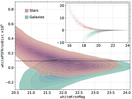
Figure 3: The distribution of $\mathtt{whitePSFKronDist}$ values for HST training set point sources (labeled stars) and extended objects (labeled galaxies) as a function of whiteKronMag. The colors and contours are the same as Figure 2. The horizontal dashed line shows the optimal threshold ($\mathtt{whitePSFKronDist}\geq 9.2\times 10^{-7}$) for resolved–unresolved classification. The upper-right inset shows a zoom-out highlighting the stark difference between stars and galaxies at the bright end.

The distribution of $\mathtt{whitePSFKronDist}(a=0.91375)$ is shown for the HST training set in Figure 3. $\mathtt{whitePSFKronDist}$ provides an excellent discriminant between bright ($\lesssim 20\,\mathrm{mag}$) point sources and extended objects. We further find that adopting a point source classification threshold of $\mathtt{whitePSFKronDist}\geq 9.2\times 10^{-7}$ produces a classification accuracy of $\sim$91%.

4.3 Random Forest Model

4.3.1 The Random Forest Algorithm

Based on its success in previous astronomical applications (e.g., Richards et al. 2012; Huppenkothen et al. 2017; Brink et al. 2013; Wright et al. 2015; Goldstein et al. 2015), including morphological classification (e.g., Vasconcellos et al. 2011; Miller et al. 2017), we adopt the RF algorithm (Breiman, 2001) for our machine learning model. In fact, following the comparison of several different algorithms it was recently found that ensemble tree-based methods, such as RF, perform best when separating stars and galaxies (Sevilla-Noarbe et al., 2018). In future work, we will consider alternative ensemble methods (such as adaptive boosting; Freund & Schapire 1997), which is found to slightly outperform RF for similar problems (Sevilla-Noarbe et al., 2018).

Briefly, RF is built on decision tree models (Quinlan, 1993) that utilize bagging (Breiman, 1996), wherein bootstrap samples of the training set are used to train each of the $N_{\mathrm{tree}}$ individual trees. Within the individual trees, only $m_{\mathrm{try}}$ randomly selected features are used to separate sources at each node, and nodes cannot be further split if there are fewer than nodesize sources in the node. The randomness introduced by both bagging and the use of $m_{\mathrm{try}}$ features reduces the variance of RF predicitions relative to single decision tree models. Final RF classifications are determined via a majority vote from each of the $N_{\mathrm{tree}}$ individual trees. Thus, RF models are capable of producing low-variance, low-bias predictions. We utilize the Python scikit-learn implementation of the RF algorithm (Pedregosa et al., 2012) in this study.

4.3.2 Feature Selection

While the RF algorithm is relatively insensitive to correlated and/or weak/uninformative features (e.g., Richards et al. 2012), we nevertheless investigate if removing features from our feature set improves the model performance. We do this via forward and backward feature selection (Guyon & Elisseeff, 2003). Forward and backward feature selection involve the iterative addition or removal of features from the model, respectively. Like Richards et al. (2012), we rank order the features for either addition or subtraction based on their RF-determined importance (Breiman, 2002). This method shows whitePSFKronDist to be the most important feature, and we find that removing features does not improve the CV FoM. We therefore include all 11 “white flux” features from §3 in the final RF model.

4.3.3 Optimizing the Model Tuning Parameters

As noted in §4.2, we optimize the RF model tuning parameters via an outter and inner 10-fold CV procedure. We perform a grid search over $N_{\mathrm{tree}}$, $m_{\mathrm{try}}$ and nodesize, and find that the FoM for the HST training set is maximized with $N_{\mathrm{tree}}=400$, $m_{\mathrm{try}}=4$, and $\mathtt{nodesize}=2$. The final model FoM is not strongly sensitive to the choice of these parameters: changing any of the optimal parameters by a factor of $\sim$2 does not decrease the optimal CV FoM, $\sim$0.71, by more than the scatter measured from the individual folds, $\sim$0.02. Finally, while a detailed comparison is presented in §5.1, we note that the RF model significantly outperforms the simple model based on the CV FoM.

5 Classification Performance

5.1 PS1, Simple, and RF Model Comparison

We assess the relative performance of the RF model by comparing it to both the PS1 and simple models. To do so, we select the subset of sources from the HST training set that have $\mathrm{det}_{i_{\mathrm{PS1}}}=1$ (the PS1 model cannot classify sources that are not detected in the $i_{\mathrm{PS1}}$ band), which results in 40,098 sources.

Figure 4 shows that the RF model and simple model provide substantial improvements over the PS1 model, with $\sim$10,000% and $\sim$9,200% respective increases in the FoM relative to the PS1 model. We additionally show Receiver Operating Characteristic (ROC) curves for the 3 models in Figure 4. ROC curves show how the true positive rate (TPR) and false positive rate (FPR) vary as a function of classification threshold. As a reminder, point sources are considered the positive class in this study. To construct ROC curves for the simple and PS1 models we vary the classification thresholds from $\mathtt{whitePSFKronDist}=4.24\times 10^{-3}$ to $-16.23\times 10^{-3}$ and $\mathtt{iPSFMag}-\mathtt{iKronMag}=5.10\;\mathrm{mag}$ to $-2.81\;\mathrm{mag}$, respectively. Figure 4 highlights the strength of the simple model approach: by using a metric that essentially captures both the difference between the PSF and Kron flux measurements and the SNR, the simple model produces much higher TPR at low FPR than the PS1 model, which does not capture information about the SNR.

Summary statistics showing the superior performance of the RF model relative to the simple and PS1 models are presented in Table 1. These statistics include the FoM, the overall classification accuracy, and the integrated area under the ROC curve (ROC AUC) of the 3 models as evaluted on the subset of HST training set sources with $i_{\mathrm{PS1}}$ detections. We use 10-fold CV to measure the summary statistics, with identical folds for each model. Strictly speaking, this CV procedure is only needed for the RF model, which needs to be re-trained for every fold, but testing the simple and PS1 models on the individual folds provides an estimate in the scatter of the final reported metrics. From Table 1 it is clear that the RF model greatly outperforms the simple and PS1 models.

Table 1: CV Results for the HST Training Set

model	FoM	Accuracy	ROC AUC
RF	0.707 $\pm$ 0.036	0.932 $\pm$ 0.003	0.973 $\pm$ 0.002
simple	0.657 $\pm$ 0.020	0.916 $\pm$ 0.003	0.937 $\pm$ 0.004
PS1	0.007 $\pm$ 0.003	0.810 $\pm$ 0.006	0.851 $\pm$ 0.006

Note. — Uncertainties represent the sample standard deviation for the 10 individual folds used in CV. For each metric, the model with the best performance is shown in bold.

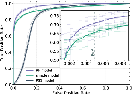
Figure 4: ROC curves comparing the relative performance of the PS1, simple, and RF models as tested by the subset of HST training set sources with $i_{\mathrm{PS1}}$ detections. The thick, solid slate gray, green, and purple lines show the ROC curves for the PS1, simple, and RF models, respectively. The light, thin lines show the ROC curves for the individual CV folds. The inset on the right shows a zoom in around FPR = 0.005, shown as a dotted vertical line, corresponding to the FoM (the PS1 model is not shown in the inset, because it has very low FoM).

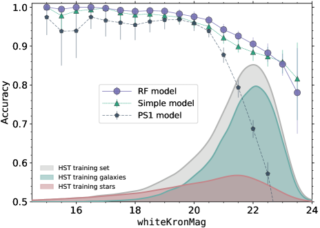
Figure 5: Model accuracy as a function of whiteKronMag evaluated on the subset of HST training set sources with $i_{\mathrm{PS1}}$ detections. Accuracy curves for the PS1, simple and RF models are shown as slate gray pentagons, green triangles, and purple circles, respectively. The bin widths are 0.5 mag, and the error bars represent the 68% interval from bootstrap resampling. Additionally, a Gaussian KDE of the PDF for the $i_{\mathrm{PS1}}$-detection subset of HST training set, as well as the point sources (labeled stars) and extended objects (labeled galaxies) in the same subset is shown in the shaded gray, red, and green regions, respectively. The amplitude of the star and galaxy PDFs have been normalized by their relative ratio compared to the full $i_{\mathrm{PS1}}$-band subset.

The classification accuracy for each model as a function of whiteKronMag is shown in 0.5 mag bins in Figure 5. The accuracies are estimated via 10-fold CV (see above) and the uncertainties represent the inter-68% interval from 100 bootstrap samples within each bin. The classification thresholds for the RF, simple, and PS1 models are 0.5, $9.2\times 10^{-7}$, and 0.05, respectively. Again, the RF and simple models provide a significant improvement over the PS1 model. The PS1 model provides classification accuracies $\gtrsim$90% for sources with $\mathtt{whiteKronMag}\lesssim 21\,\mathrm{mag}$, but precipitously declines for fainter sources. The RF and simple models have similar curves with the RF model performing slightly better, as is to be expected given that the RF model uses 10 additional features beyond whitePSFKronDist.

5.2 Model Evaluation via an Independent Test Set

Table 2: SDSS Test Set Metrics

model	FoM	Accuracy	ROC AUC
RF	0.843 $\pm$ 0.001	0.9625 $\pm$ 0.0001	0.98713 $\pm$ 0.00007
simple	0.798 $\pm$ 0.002	0.9557 $\pm$ 0.0001	0.98503 $\pm$ 0.00008
PS1	0.290 $\pm$ 0.004	0.9612 $\pm$ 0.0001	0.98411 $\pm$ 0.00007
SDSS	0.777 $\pm$ 0.003	0.9713 $\pm$ 0.0001	0.98660 $\pm$ 0.00008

Note. — Uncertainties represent the sample standard deviation for 100 bootstrap samples of the SDSS test set. For each metric, the model with the best performance is shown in bold.

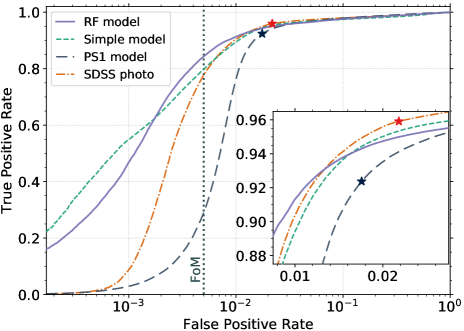
Figure 6: ROC curves comparing the relative performance of the SDSS (orange dot-dashed line), PS1 (slate grey dashed line), simple (green dotted line), and RF (solid purple) models as tested by the SDSS test set. Note that the FPR is shown on a logarithmic scale. The vertical dotted line shows $\mathrm{FPR}=0.005$, corresponding to the FoM. The inset shows a zoom in around the region where the ROC curves cross (see text for further details). The black and red stars show the FPR and TPR if adopting the PS1 model and SDSS photo classification cuts, respectively. The RF model delivers the highest FoM.

While CV on the HST training set shows that the RF model outperforms the alternatives, here, we test each of the previous models with the SDSS training set, which provides an independent set of $\sim$3.8$\times 10^{6}$ sources with high-confidence labels. Additionally, the use of SDSS spectra allows us to compare our new models to the classifications from the SDSS photo pipeline, hereafter the SDSS model, which soundly outperformed the PTF point source classification model (Miller et al., 2017). We create an ROC curve for the SDSS model by thresholding on the ratio of PSF flux to cmodel flux measured in the SDSS images (see Miller et al. 2017 for more details).

To compare the 4 models, we evaluate the performance of each model on the subset of SDSS training set sources that have $i_{\mathrm{PS1}}$ detections (to compare with the PS1 model) and SDSS photo classifications (to compare with the SDSS model). We further exclude QSOs with $z<1$ (= 133,856 sources; QSOs are typically considered point sources but low-$z$ QSOs can have resolved host galaxies; see Miller et al. 2017), and galaxies with $z<10^{-4}$ (= 13,261 sources; such low $z$ is only expected in the local group meaning most of these classifications are likely spurious). In total, this subsample (hereafter the SDSS test set) includes 3,592,940 sources from the SDSS training set.

ROC curves for the RF, simple, PS1, and SDSS models, as measured by the SDSS test set, are shown in Figure 6. The FoM for the PS1, simple, and RF models is higher as tested by SDSS spectroscopic sources because the SDSS training set contains brighter, higher SNR (and hence easier to classify) sources. As before, we find that the FoM for the RF model is superior to the alternatives. Interestingly, we also find that the ROC curves cross, and that the SDSS model provides the largest TPR for $\mathrm{FPR}\gtrsim 0.015$. That the RF and SDSS curves cross suggests that there may be regimes where the SDSS photo classifications are superior to the RF model. Below, we argue that a bias in the SDSS training set is amplified by a bias in the SDSS photo classification, which is why these curves cross.

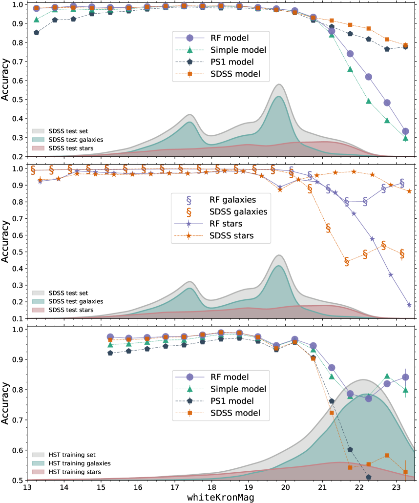
Figure 7: Model accuracy for the RF (purple circles), simple (green triangles), PS1 (slate gray pentagons), and SDSS (orange squares) models as a function of whiteKronMag evaluated on the SDSS test set. The bin widths are 0.5 mag, and the error bars represent the central 68% interval from bootstrap resampling within each bin. Top: Model accuracy curves for the SDSS test set. This panel also shows a Gaussian KDE of the PDF for the SDSS test set, as well as the point sources (labeled stars) and extended objects (labeled galaxies) in the SDSS test set in the shaded gray, red, and green regions, respectively. The amplitude of the point source and extended object PDFs have been normalized by their relative fraction of the full test set. Middle: SDSS test set accuracy curves for individual point sources and extended objects, equivalent to the TPR and TNR, respectively, as classified by the RF and SDSS models (the simple and PS1 models are not shown for clarity). Note – all 3 panels have the same bin centers, though here the markers are slightly offset for clarity. The SDSS model classifies faint point sources correctly, but has poor performance on faint extended objects, while the opposite is true for the RF model. Bottom: The accuracy curves for all 4 models following the bootstrap procedure (described in the text) to correct for the SDSS test set bias whereby point sources outnumber extended objects at $\mathtt{whiteKronMag}\gtrsim 20.5\,\mathrm{mag}$. The PDFs shown in this panel are derived from KDEs of the HST training set (as in Figure 5). After correcting for the SDSS test set number count bias, the RF and simple models produce more accurate classifications of faint sources than the SDSS and PS1 models.

Accuracy curves for each of the 4 models, as evaluated on the SDSS test set, is shown in the top panel of Figure 7. The RF, simple, and SDSS models all provide near-perfect ($\geq 97.5$%) accuracy down to whiteKronMag $\approx 20\,\mathrm{mag}$. The PS1 model is similar, though has a noticably worse performance for the brightest (whiteKronMag $\lesssim 14.5\,\mathrm{mag}$) sources. For sources with $\mathtt{whiteKronMag}>21\,\mathrm{mag}$, the SDSS and PS1 models provide far more accurate classifications than the RF and simple models. In this faint regime, the SDSS test set is dominated by point sources (top panel, Figure 7). This is counter to what is observed in nature (at high galactic latitudes), as extended object number counts exceed those of point sources around $r\gtrsim 20\,\mathrm{mag}$ (e.g., Yasuda et al. 2001; Shanks et al. 2015). This bias in the SDSS test set is due to the SDSS targeting proclivity for luminous red galaxies (LRGs) at $z\approx 0.5$ (e.g., Eisenstein et al. 2001) and faint $z\approx 2.7$ QSOs (e.g., Ross et al. 2012).

In addition to this bias in the SDSS test set, the SDSS (and PS1) model are biased towards classifying faint resolved sources as unresolved. This is due to the hard cut on a single value of the PSF to cModel (or Kron for PS1) flux ratio. The reason for this can easily be seen in the top left panel of Figure 2, where a classification cut at $\mathtt{whitePSFKronRatio}=0.875$ (equivalent to the SDSS cut) correctly identifies nearly all of the point sources, but does a particularly bad job with the faintest extended objects. At low SNR the large scatter in flux ratio measurements results in many misclassifications.

We show further evidence for this classification bias in the middle panel of Figure 7, which shows the accuracy with which individual extended sources and point sources in the SDSS test set are classified by the RF and SDSS models (curves for the simple and PS1 models show similar trends as the RF and SDSS models, respectively, but are omitted for clarity). For faint ($\mathtt{whitePSFKronRatio}>21\,\mathrm{mag}$) sources, the SDSS model performs well on point sources ($\mathrm{TPR}\gtrsim 0.9$) and poorly on extended sources ($\mathrm{TNR}\approx 0.5$). The opposite is true for the RF model, with $\mathrm{TNR}\gtrsim 0.8$ and a TPR that declines to $\sim$0.2 for the faintest SDSS test set sources. Thus, for faint sources the RF model is slightly biased towards resolved object classifications, however, this bias is in line with what is observed in nature. These classification biases, taken together with the SDSS test set bias towards point sources at the faint end, explain why the accuracy curves for the SDSS (and PS1) model outperform the RF (and simple) model (and also why their ROC curves cross in Figure 6).

The bottom panel of Figure 7 shows that after correcting for the number counts bias in the SDSS test set, the RF and simple models greatly outperform the SDSS and PS1 models. We correct for the number count bias via bootstrap resampling, whereby we select a subset of point sources and extended objects from the SDSS test set to match the ratio of point sources to extended objects in the HST training set. The HST training set, which is selected photometrically, should serve as a far better approximation for the relative number counts of point sources and extended objects at high-Galactic latitudes than the SDSS test set. The bootstrap occurs in bins of width 0.5 mag from whiteKronmag = 15 mag to 23.5 mag, and we select 100 bootstrap samples within each bin. In each bin the size of the bootstrap sample is set by the underrepresented class within the SDSS test set. For example, if the HST training set has an unresolved–resolved number ratio of 0.6 and in the same bin the SDSS test set has 1000 point sources and 4000 extended objects, then 1000 point sources and 1667 extended objects will be selected in each bootstrap sample. Similarly, for an unresolved–resolved number ratio of 0.25 in a bin with 800 point sources and 1000 extended objects, then 250 point sources and 1000 extended objects will be selected.

Correcting for the number counts bias in the SDSS test set reveals some interesting trends: as was the case prior to correction all 4 models perform similarly well for bright (whiteKronMag $\lesssim 20\,\mathrm{mag}$) sources. However, for fainter sources the RF and simple models significantly outperform the SDSS and PS1 models. The bottom panel of Figure 7 also shows a kink at whiteKronMag $\approx 19.75\,\mathrm{mag}$. As first explained in Miller et al. (2017), this kink is due to blended, faint red stars that were targeted as candidate LRGs. Thus, spectra show these sources to be stellar, while they appear extended in imaging data. Finally, we conclude that for source distributions similar to what is observed in nature, the RF model outperforms the alternatives discussed here in both the FoM and the overall accuracy.

6 The PS1 Catalog Deployed: Integration in ZTF

6.1 The Zwicky Transient Facility

While we have developed a general model to identify point sources, the resulting RF classifications have been specifically deployed in the Zwicky Transient Facility (ZTF; Bellm et al. 2018; Dekany et al. 2018) real-time pipeline (Masci et al., 2018). Briefly, ZTF is the next-generation Palomar time-domain survey, which succeeds PTF (Rau et al., 2009; Law et al., 2009) and the intermediate Palomar Transient Factory (iPTF; Kulkarni 2013). ZTF, with its 47 deg² field of view, can scan at a rate $\sim$15$\times$ faster than PTF/iPTF ($>3{,}750\,\deg^{2}\,\mathrm{hr}^{-1}$) to a depth of $R_{\mathrm{ZTF}}\approx 20.4$ mag ($5\sigma$). ZTF will observe the entire sky with $\delta>-30^{\circ}$ $\sim$300 times per year, with publicly distributed alerts on newly observed positional or flux variability released in near real time (Patterson et al., 2018).

6.2 Integration in the ZTF Alert Stream

An initial, and pressing, question for filtering the ZTF alert stream, is: does the newly identified variable have a Galactic or extragalactic origin? Hence the need for a resolved–unresolved model, and in particular, one that is deeper than typical ZTF observations (to identify faint stars flaring above the ZTF detection limit). While ZTF will address many science objectives (e.g., Graham et al. 2018), a primary motivation is the search for fast transients, especially kilonovae (KNe), the result of merging binary neutron stars. If the proximity and sky location of a KN is favorable, these events can be detected via gravitational waves (e.g., GW 170817, see Abbott et al. 2017 and references therein). The search for KNe is plagued by significant foreground contamination in the form of stellar flares and/or orbital modulation (e.g., Kulkarni & Rau 2006; Berger et al. 2012; Kasliwal et al. 2016). Our PS1 RF model enables the systematic removal of faint stars from extragalactic candidate lists, and our adopted FoM ensures that nearly every galaxy ($\sim$99.5%) is searched for candidate KNe.

Newly discovered ZTF candidates are associated with the 3 nearest PS1 counterparts within 30″ in the real-time alert packets (Masci et al., 2018). Counterparts are selected from ZTF calibration sources, which includes all PS1 MeanObject table sources with $\mathtt{nDetections}\geq 3$. Thus, to create the ZTF–PS1 point source catalog we selected sources from the StackObjectAttributes table with $\mathtt{nDetections}\geq 3$, and merged these classifications with the ZTF calibration sources. Ultimately, non-unique sources (i.e., if a single objID corresponds to multiple rows with primaryDetection = 1) are excluded from the classification catalog.

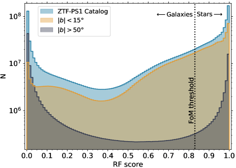
Figure 8: The distribution of RF classification score for all sources in the ZTF–PS1 point source catalog. Note that the number counts are shown on a log scale. The vertical dotted line shows the FoM-optimized classification threshold, sources to the right of the line are classified as point sources. The full catalog is shown in blue, while Galactic plane sources ($|b|<15^{\circ}$) are shown in orange, and high galactic latitude sources ($|b|>50^{\circ}$) are shown in grey. Ambiguous classifications ($0.2\lesssim\mathrm{RF\;score}\lesssim 0.8$) in the catalog are dominated by sources in the Galactic plane.

In total, there are 1,484,281,394 PS1 sources with RF classifications. A histogram showing the distribution of the final RF classifications is shown in Figure 8. The thresholds appropriate for identifying point-source counterparts to the ZTF candidates are reported in Table 3 (note that these thresholds apply to $\mathtt{nDetections}\geq 3$ sources). Of the $\sim$1.5$\times 10^{9}$ sources in the ZTF–PS1 catalog, 734,476,355 ($\sim$50%) are classified as point sources using the FoM-optimized classification threshold of 0.83.

Table 3: Classification thresholds for the ZTF–PS1 Catalog.

Selection criteria	$N$	Accuracy	FPR	0.005	0.01	0.02	0.05	0.1
All sources	35,007	$93.9\pm 0.1$%	TPR	$0.734\,^{+0.012}_{-0.014}$	$0.792\,^{+0.010}_{-0.009}$	$0.843\,^{+0.008}_{-0.008}$	$0.904\,^{+0.005}_{-0.005}$	$0.947\,^{+0.004}_{-0.004}$
			Threshold	$0.829\,^{+0.018}_{-0.010}$	$0.724\,^{+0.016}_{-0.014}$	$0.597\,^{+0.014}_{-0.010}$	$0.397\,^{+0.008}_{-0.006}$	$0.224\,^{+0.006}_{-0.004}$
$\mathtt{rKronMag}<21$	13,570	$98.0\pm 0.1$%	TPR	$0.797\,^{+0.146}_{-0.101}$	$0.964\,^{+0.007}_{-0.014}$	$0.980\,^{+0.003}_{-0.004}$	$0.989\,^{+0.003}_{-0.002}$	$0.995\,^{+0.002}_{-0.001}$
			Threshold	$0.970\,^{+0.015}_{-0.043}$	$0.645\,^{+0.115}_{-0.041}$	$0.406\,^{+0.048}_{-0.014}$	$0.170\,^{+0.018}_{-0.011}$	$0.069\,^{+0.006}_{-0.003}$
$\mathtt{rKronMag}<20$	6,956	$99.0\pm 0.1$%	TPR	$0.697\,^{+0.197}_{-0.219}$	$0.954\,^{+0.038}_{-0.082}$	$0.994\,^{+0.002}_{-0.002}$	$0.997\,^{+0.002}_{-0.002}$	$0.998\,^{+0.001}_{-0.001}$
			Threshold	$0.993\,^{+0.005}_{-0.015}$	$0.923\,^{+0.052}_{-0.328}$	$0.339\,^{+0.082}_{-0.050}$	$0.132\,^{+0.036}_{-0.021}$	$0.047\,^{+0.006}_{-0.005}$

Note. — 10-fold CV is performed on the entire HST training set, but the metrics reported here include only sources that satisfy the selection criteria defined by the first column and $\mathtt{nDetections}\geq 3$. The reported uncertainties represent the central 90% interval from 100 bootstrap resamples of the training set.

Figure 8 additionally shows that most of the point sources in the catalog are located in the Galactic plane, most of the (high-confidence) extended objects are outside the plane, and (unsurprisingly) that classification is more challenging in regions of high stellar density. At high galactic latitudes ($|b|>50^{\circ}$), where the distribution of sources is similar to the HST training set, sources are well segregated (RF score $\approx$0 or 1), with very few ambiguous classifications ($0.2\lesssim\mathrm{RF\;score}\lesssim 0.8$). The Galactic plane region ($|b|<15^{\circ}$) dominates the ambiguous classifications in the ZTF–PS1 point source catalog. We attribute this to a lack of reliable training data in high-stellar-density regions, and significantly more blending, which results in point sources appearing extended. Thus, identifying stellar sources in the Galactic plane likely requires a lower threshold than the FoM-optimized classification value. The final tuning of the resolved–unresolved classification thresholds is a critical early step in the filtering of ZTF candidates (e.g., Kasliwal et al. 2018), which is necessary to optimize follow-up of newly discovered transients.

6.3 Verifying, and Updating, the Catalog with Gaia

The Gaia satellite (Gaia Collaboration et al., 2016) is currently conducting an all-sky survey that provides unprecedented astrometric accuracy in measuring the positions, parallaxes, and proper motions of $\sim$1.3 billion sources (Gaia Collaboration et al. 2018a; an additional $\sim$0.3 billion sources have just position measurements). The Gaia selection function is biased against resolved galaxies (Gaia Collaboration et al., 2016), so it cannot provide a symmetric test of the ZTF–PS1 catalog. Nevertheless, Gaia has identified hundreds of millions of stars that can be used to test our classifications.

Given that Gaia does not classify the sources it detects as either resolved or unresolved, we test the ZTF–PS1 catalog by selecting a pure sample of Gaia stars based on high-significance parallax, $\varpi$, and proper motion, $\mu$, measurements. We define the $\varpi$ significance as $\varpi$/$\sigma_{\varpi}$ (called parallax_over_error in the Gaia database). We obtain the total proper motion $\mu$ by adding the proper motion in Right Ascension $\mu_{\alpha\ast}$ and Declination $\mu_{\delta}$ (pmra and pmdec in the database, respectively) in quadrature. The uncertainty in the total proper motion, $\sigma_{\mu}$, is calculated via the proper motion uncertainties in Right Ascension, $\sigma_{\mu_{\alpha\ast}}$, and Declination, $\sigma_{\mu_{\delta}}$, while accounting for the correlation coefficient between $\mu_{\alpha\ast}$ and $\mu_{\delta}$, $\rho(\mu_{\alpha\ast}\mu_{\delta})$:

$$\sigma_{\mu}^{2}=\frac{\mu_{\alpha\ast}^{2}}{\mu^{2}}\sigma_{\mu_{\alpha\ast}}^{2}+\frac{\mu_{\delta}^{2}}{\mu^{2}}\sigma_{\mu_{\delta}}^{2}+2\frac{\mu_{\alpha\ast}\mu_{\delta}}{\mu^{2}}\rho(\mu_{\alpha\ast}\mu_{\delta})\sigma_{\mu_{\alpha\ast}}\sigma_{\mu_{\delta}}.$$

The proper motion signficance is then defined as $\mu/\sigma_{\mu}$.

To determine the threshold for “high significance” in $\varpi$ and $\mu$ we use faint stars and activate galactic nuclei (AGN), respectively. In Lindegren et al. (2018), a sample of $\sim$5.5$\times 10^{5}$ AGN with Gaia observations were identified, and the cosmological distances to these sources mean they should have extremely small parallaxes and proper motions. We find that 99.997% of these AGN have $\mu$ significance $<5.62$, and the highest $\mu$ significance in the entire AGN sample is $\sim$7.42. Thus, we apply a conservative cut of 7.5 on $\mu$ significance to select a pure set of stars with little contamination from extended, extragalactic objects.

The AGN sample is not sufficient for defining a cut on $\varpi$ significance, because Lindegren et al. (2018) require $\varpi$/$\sigma_{\varpi}<5$. Instead, we use the 20,568,254 Gaia sources with $\varpi$ and $\mu$ measurments, $20.5\,\mathrm{mag}\leq G\leq 21\,\mathrm{mag}$, where $G$ is the mean brightness measured by Gaia in the $G$ filter, and that pass the cuts defined by Eqn. (C.1) and (C.2) in Lindegren et al. (2018). These cuts are designed to remove low-confidence parallax measurements in regions of high stellar density. The low SNR detections for these Gaia sources provide an estimate of the scatter of the parallax significance, as they are too faint for high-significance detections. Looking at the full distribution of parallax significance for these faint sources we find that 99.997% have parallax significance $<7.94$. Again, we apply a conservative cut of parallax significance $\geq$8 to select bonafide stars from the Gaia data.

Figure 9: The distribution of RF classification score for sources in the ZTF–PS1 star–galaxy catalog selected as high-probability stars from Gaia due to their significant proper motion (see text for further details). Note that the number counts are shown on a log scale. The vertical dotted line shows the FoM-optimized classification threshold, sources to the right of the line are classified as stars. The full catalog is shown in blue, while Galactic plane sources ($|b|<10^{\circ}$) are shown in orange, and high galactic latitude sources ($|b|>30^{\circ}$) are shown in grey. Less than 0.25% of these stars have $\mathrm{RF\;score}\lesssim 0.5$.

Using the existing crossmatch between Gaia and PS1, we have identified 38,764,553 and 234,176,264 high-confidence stars that pass the cuts defined by Eqn. (C.1) and (C.2) in Lindegren et al. (2018) and have parallax significance $\geq 8$ or proper motion significance $\geq 7.5$, respectively. Of these, 35,599,830 and 225,682,755 have respective counterparts in the ZTF–PS1 catalog (the respective differences of 3,164,723 and 8,493,509 correspond to sources with either 0 or $>$1 entries in the PS1 StackObjectThin table). For the proper motion selected stars, we show the distribution of RF classification scores for these stellar objects in Figure 9. It is clear from Figure 9 that the vast majority of stars are classified correctly. Half of the stars selected via proper motion have $\mathrm{RF\;score}\geq 0.99$, while 98.1% have $\mathrm{RF\;score}\geq 0.83$, the FoM classification threshold, and 99.75% have $\mathrm{RF\;score}\geq 0.5$, the traditional binary classification threshold. The percentages are even higher for the parallax-selected sample. These calssification results are significantly better than those reported in Table 3, which makes sense given that this high significance Gaia sample is much brighter than the sources in the HST training set (median brightness $G=18.0\,\mathrm{mag}$, 95^th percentile brightness $G=19.7\,\mathrm{mag}$). Nevertheless, we conclude that the Gaia data confirms that our method does an excellent job of identifying point sources.

Finally, the 8,520,167 sources selected by either the parallax or proper motion cuts described above that do not have counterparts in the ZTF–PS1 catalog are assigned an RF classification score of 1 in the ZTF database. Thus, new transient candidates with positions consistent with these sources will be flagged as likely stars.

7 Summary and Conclusions

We have presented the development of a large ($\sim$1.5$\times 10^{9}$), deep ($m\lesssim 23.5\,\mathrm{mag}$) catalog of point sources and extended objects based on PS1 data. We classify these sources using a machine learning framework built on a RF model. The RF model is trained using 47,093 PS1 sources with HST COSMOS morphological classifications.

To construct the RF model, we introduced “white flux” features, which correspond to a weighted mean of the relevant features over the $grizy_{\mathrm{PS1}}$ filters in which a source is detected. The “white flux” features allow us to classify all PS1 sources, irrespective of the filters in which the source was detected or the line-of-sight reddenning. One of these newly created features, whitePSFKronDist, is useful on its own for separating stars and galaxies. Unlike a hard cut on the PSF and Kron flux ratio, as is employed by the SDSS and PS1 models, whitePSFKronDist retains knowledge of the SNR and therefore can provide higher confidence classifications. From whitePSFKronDist we created the simple model, which does a good job of separating point sources and extended objects. Ultimately, the 11 “white flux” features, used in combination with the RF algorithm, provide the best classification of PS1 sources.

CV on the HST training set shows that the RF (FoM$=0.71$) and simple (FoM$=0.657$) models greatly outperform the PS1 (FoM$=0.007$) model. For faint sources ($\mathtt{whiteKronMag}>20$ mag) the PS1 model misclassifies many extended objects as point sources, while both the simple and RF models provide overall classification accuracies $\gtrsim 85$% as faint as $\mathtt{whiteKronMag}=23$ mag.

We find that when evaluated with the SDSS test set, the SDSS and PS1 models provide more accurate classifications than the RF and simple models, especially for faint ($\mathtt{whiteKronMag}\gtrsim 21$ mag) sources. This reversal, relative to the HST training set results, can be attributed to a bias in the SDSS test set and the SDSS classification model. In the SDSS test set point sources outnumber galaxies at the faint end, which is counter to what is observed (at high galactic latitudes). Furthermore, the SDSS and PS1 models, which utilize a hard cut on flux ratios, are likely to classify low SNR sources as point sources. Together, these effects amplify the perceived performance of the SDSS and PS1 models. Using a bootstrap resampling procedure, we correct for the relative number counts bias in the SDSS test set, and find that the RF and simple models outperform the SDSS and PS1 models, both in terms of FoM and overall accuracy. Thus, of the 4 models considered in this study the RF model is superior to all others.

We have deployed the RF model in support of the ZTF real-time pipeline, resulting in the classification of $\sim$1.5$\times 10^{9}$ sources. The catalog is dominated by point sources in the vicinity of the Galactic plane, though we find that there are more extended objects than point sources at high galactic latitudes, as is expected at the depth of PS1. ZTF is currently producing public alerts for newly discovered variability, and the ZTF–PS1 catalog is essential for removing the numerous foreground of stellar flares, false positives in the search for fast transients and KNe, from the extragalactic alert stream. The final ZTF–PS1 catalog is available at MAST via http://dx.doi.org/10.17909/t9-xjrf-7g34 (catalog doi:10.17909/t9-xjrf-7g34).

Moving forward, future data releases and additional scrutiny of Gaia data will significantly increase the fidelity of the PS1 resolved–unresolved classification model. The HST training set has very few bright sources and no sources at low Galactic latitudes, leading to less confident classifications in these regions (see Figure 8). As a space-based observatory, Gaia will resolve many stellar blends in the Galactic plane and identify millions of stars brighter than 16 mag. Many of the ambiguous classifications in the ZTF–PS1 catalog (see §6) will be directly identified as stars due to their high proper motions and parallaxes (similar to the analysis in 6.3, though future Gaia observations will lead to even better precision). As previously noted, Gaia does not downlink measurements for extended sources. Thus, while Gaia would allow us to increase the size of our training set by many orders of magnitude, it would also introduce a significant class imbalance. Correcting for the lack of galaxies would require new approaches beyond those described here. It should also be noted that Gaia alone is not sufficient for our purposes, as it only detects sources with $G\lesssim 21$ mag, which does not include the faint, flaring stars that we expect to be the primary false positive in the search for fast transients. Nevertheless, our ability to now merge several $\sim$all-sky surveys provides unprecedented power in the classification of astronomical sources. This power is particularly important for improving the scientific output and follow-up efficiency of time-domain surveys.

References

- Abbott et al. (2017) Abbott, B. P., Abbott, R., Abbott, T. D., et al. 2017, ApJ, 848, L13
- Astropy Collaboration et al. (2013) Astropy Collaboration, Robitaille, T. P., Tollerud, E. J., et al. 2013, A&A, 558, A33
- Bellm et al. (2018) Bellm, E., Kulkarni, S., & Graham, M. J., e. a. 2018, PASP, 999, 99
- Belokurov et al. (2006) Belokurov, V., Zucker, D. B., Evans, N. W., et al. 2006, ApJ, 642, L137
- Berger et al. (2012) Berger, E., Chornock, R., Lunnan, R., et al. 2012, ApJ, 755, L29
- Bertin & Arnouts (1996) Bertin, E., & Arnouts, S. 1996, A&AS, 117, 393
- Bevington & Robinson (2003) Bevington, P. R., & Robinson, D. K. 2003, Data reduction and error analysis for the physical sciences
- Breiman (1996) Breiman, L. 1996, Machine Learning, 24, 123
- Breiman (2001) —. 2001, Machine Learning, 45, 5
- Breiman (2002) —. 2002, Statistics Department University of California Berkeley, CA, USA.
- Brink et al. (2013) Brink, H., Richards, J. W., Poznanski, D., et al. 2013, MNRAS, 435, 1047
- Chambers et al. (2016) Chambers, K. C., Magnier, E. A., Metcalfe, N., et al. 2016, ArXiv e-prints
- Dekany et al. (2018) Dekany, R. G., Smith, R. M., & Bellm, E., e. a. 2018, PASP, 999, 99
- Eisenstein et al. (2001) Eisenstein, D. J., Annis, J., Gunn, J. E., et al. 2001, AJ, 122, 2267
- Flewelling et al. (2016) Flewelling, H. A., Magnier, E. A., Chambers, K. C., et al. 2016, ArXiv e-prints
- Freund & Schapire (1997) Freund, Y., & Schapire, R. E. 1997, A Decision-Theoretic Generalization of on-Line Learning and an Application to Boosting, ,
- Gaia Collaboration et al. (2018a) Gaia Collaboration, Brown, A. G. A., Vallenari, A., et al. 2018a, ArXiv e-prints, arXiv:1804.09365
- Gaia Collaboration et al. (2018b) —. 2018b, ArXiv e-prints, arXiv:1804.09365
- Gaia Collaboration et al. (2016) Gaia Collaboration, Prusti, T., de Bruijne, J. H. J., et al. 2016, A&A, 595, A1
- Gaia Collaboration et al. (2018c) Gaia Collaboration, Babusiaux, C., van Leeuwen, F., et al. 2018c, A&A, arXiv:1804.09378. https://doi.org/10.1051/0004-6361/201832843
- Goldstein et al. (2015) Goldstein, D. A., D’Andrea, C. B., Fischer, J. A., et al. 2015, AJ, 150, 82
- Graham et al. (2018) Graham, F., Kulkarni, S., & Bellm, E., e. a. 2018, PASP, 999, 99
- Green et al. (2015) Green, G. M., Schlafly, E. F., Finkbeiner, D. P., et al. 2015, ApJ, 810, 25
- Guyon & Elisseeff (2003) Guyon, I., & Elisseeff, A. 2003, J. Mach. Learn. Res., 3, 1157. http://dl.acm.org/citation.cfm?id=944919.944968
- Ho et al. (2015) Ho, S., Agarwal, N., Myers, A. D., et al. 2015, J. Cosmology Astropart. Phys, 5, 040
- Hodapp et al. (2004) Hodapp, K. W., Kaiser, N., Aussel, H., et al. 2004, Astronomische Nachrichten, 325, 636
- Hunter (2007) Hunter, J. D. 2007, Computing In Science & Engineering, 9, 90
- Huppenkothen et al. (2017) Huppenkothen, D., Heil, L. M., Hogg, D. W., & Mueller, A. 2017, MNRAS, 466, 2364
- Jones et al. (2001–) Jones, E., Oliphant, T., Peterson, P., et al. 2001–, SciPy: Open source scientific tools for Python, , , [Online; accessed ¡today¿]. http://www.scipy.org/
- Kasliwal et al. (2018) Kasliwal, F., Kulkarni, S., & friends. 2018, PASP, 999, 99
- Kasliwal et al. (2016) Kasliwal, M. M., Cenko, S. B., Singer, L. P., et al. 2016, ApJ, 2016, L24
- Kron (1980) Kron, R. G. 1980, ApJS, 43, 305
- Kulkarni (2013) Kulkarni, S. R. 2013, The Astronomer’s Telegram, 4807
- Kulkarni & Rau (2006) Kulkarni, S. R., & Rau, A. 2006, ApJ, 644, L63
- Law et al. (2009) Law, N. M., Kulkarni, S. R., Dekany, R. G., et al. 2009, PASP, 121, 1395
- Leauthaud et al. (2007) Leauthaud, A., Massey, R., Kneib, J.-P., et al. 2007, ApJS, 172, 219
- Lindegren et al. (2018) Lindegren, L., Hernandez, J., Bombrun, A., et al. 2018, A&A, arXiv:1804.09366. https://doi.org/10.1051/0004-6361/201832727
- Loveday et al. (2012) Loveday, J., Norberg, P., Baldry, I. K., et al. 2012, MNRAS, 420, 1239
- Lupton et al. (2001) Lupton, R., Gunn, J. E., Ivezić, Z., Knapp, G. R., & Kent, S. 2001, in Astronomical Society of the Pacific Conference Series, Vol. 238, Astronomical Data Analysis Software and Systems X, ed. F. R. Harnden, Jr., F. A. Primini, & H. E. Payne, 269
- Magnier et al. (2016a) Magnier, E. A., Chambers, K. C., Flewelling, H. A., et al. 2016a, ArXiv e-prints, arXiv:1612.05240
- Magnier et al. (2016b) Magnier, E. A., Sweeney, W. E., Chambers, K. C., et al. 2016b, ArXiv e-prints, arXiv:1612.05244
- Marrese et al. (2017) Marrese, P. M., Marinoni, S., Fabrizio, M., & Giuffrida, G. 2017, A&A, 607, A105
- Masci et al. (2018) Masci, F., Laher, R., & Bellm, E., e. a. 2018, PASP, 999, 99
- McKinney (2010) McKinney, W. 2010, in Proceedings of the 9th Python in Science Conference, ed. S. van der Walt & J. Millman, 51 – 56
- Miller et al. (2017) Miller, A. A., Kulkarni, M. K., Cao, Y., et al. 2017, AJ, 153, 73
- Moorman et al. (2015) Moorman, C. M., Vogeley, M. S., Hoyle, F., et al. 2015, ApJ, 810, 108
- Patterson et al. (2018) Patterson, F., Kulkarni, S., & friends. 2018, PASP, 999, 99
- Pedregosa et al. (2012) Pedregosa, F., Varoquaux, G., Gramfort, A., et al. 2012, Journal of Machine Learning Research, 12
- Quinlan (1993) Quinlan, J. R. 1993, C 4.5: Programs for machine learning (The Morgan Kaufmann Series in Machine Learning, San Mateo, CA: Morgan Kaufmann)
- Rau et al. (2009) Rau, A., Kulkarni, S. R., Law, N. M., et al. 2009, PASP, 121, 1334
- Richards et al. (2012) Richards, J. W., Starr, D. L., Miller, A. A., et al. 2012, ApJS, 203, 32
- Ross et al. (2011) Ross, A. J., Ho, S., Cuesta, A. J., et al. 2011, MNRAS, 417, 1350
- Ross et al. (2012) Ross, N. P., Myers, A. D., Sheldon, E. S., et al. 2012, ApJS, 199, 3
- Schlafly et al. (2012) Schlafly, E. F., Finkbeiner, D. P., Jurić, M., et al. 2012, ApJ, 756, 158
- Scolnic et al. (2018) Scolnic, D., Kessler, R., Brout, D., et al. 2018, ApJ, 852, L3
- Sérsic (1963) Sérsic, J. L. 1963, Boletin de la Asociacion Argentina de Astronomia La Plata Argentina, 6, 41
- Sevilla-Noarbe et al. (2018) Sevilla-Noarbe, I., Hoyle, B., Marchã, M. J., et al. 2018, ArXiv e-prints, arXiv:1805.02427
- Shanks et al. (2015) Shanks, T., Metcalfe, N., Chehade, B., et al. 2015, MNRAS, 451, 4238
- Soumagnac et al. (2015) Soumagnac, M. T., Abdalla, F. B., Lahav, O., et al. 2015, MNRAS, 2015, 666
- Tonry et al. (2012) Tonry, J. L., Stubbs, C. W., Lykke, K. R., et al. 2012, ApJ, 750, 99
- Vasconcellos et al. (2011) Vasconcellos, E. C., de Carvalho, R. R., Gal, R. R., et al. 2011, AJ, 141
- Wright et al. (2015) Wright, D. E., Smartt, S. J., Smith, K. W., et al. 2015, MNRAS, 449, 451
- Yasuda et al. (2001) Yasuda, N., Fukugita, M., Narayanan, V. K., et al. 2001, AJ, 122, 1104
- York et al. (2000) York, D. G., Adelman, J., Anderson, Jr., J. E., et al. 2000, AJ, 120, 1579