Exponentiated Gradient vs. Meets Gradient Descent

Abstract

The (stochastic) gradient descent and the multiplicative update method are probably the most popular algorithms in machine learning. We introduce and study a new regularization which provides a unification of the additive and multiplicative updates. This regularization is derived from an hyperbolic analogue of the entropy function, which we call hypentropy. It is motivated by a natural extension of the multiplicative update to negative numbers. The hypentropy has a natural spectral counterpart which we use to derive a family of matrix-based updates that bridge gradient methods and the multiplicative method for matrices. While the latter is only applicable to positive semi-definite matrices, the spectral hypentropy method can naturally be used with general rectangular matrices. We analyze the new family of updates by deriving tight regret bounds. We study empirically the applicability of the new update for settings such as multiclass learning, in which the parameters constitute a general rectangular matrix.

1 Introduction

Algorithms for online learning can morally be divided into two camps. On one side is the additive gradient update. Additive gradient-based stochastic methods are the most commonly used approach for learning the parameters of shallow and deep models alike. On the other side stands the multiplicative update method. It is somewhat less glamorous, nonetheless a fundamental primitive in game theory and machine learning, and was rediscovered repeatedly in a variety of algorithmic settings (Arora et al., 2012). Both additive and multiplicative updates can be seen as special cases of a more general technique of learning with regularization. General frameworks for regularization were developed in online learning, dubbed Follow-The-Regularized-Leader and in convex optimization as the Mirrored Decent algorithms, see more below.

Notable attempts were made to unify different regularization techniques, in particular between the multiplicative and additive update methods Kivinen and Warmuth (1997). For example, AdaGrad Duchi et al. (2011) stemmed from a theoretical study of learning the best regularization in hindsight. As the name implies, the $p$-norm update Grove et al. (2001); Gentile (2003) uses the squared $p$-norm of the parameters as a regularization. By varying the order of the norm between regret bounds that are characteristic of additive and multiplicative updates.

We study a new, arguably more natural, family of regularization which “interpolates” between additive and multiplicative forms. We analyze its performance both experimentally, and theoretically to obtain tight regret bounds in the online learning paradigm. The motivation for this interpolation stems from the extension of the multiplicative update to negative weights. Instead of using the so called EG$\pm$ trick”, a term coined by Warmuth , which simulates arbitrary weights through duplication to positive and negative components, we use a direct approach. To do so we introduce the hyperbolic regularization with a single temperature-like hyperparameter. Varying the hyperparameter yields regret bounds that translate between those akin to additive, and multiplicative, update rules.

As a natural next step, we investigate the spectral analogue of the hypentropy function. We show that the spectral hypentropy is strongly-convex with respect to the Euclidean or trace norms, again as a function of the single interpolation parameter. The spectral hypentropy yields updates that can be viewed as interpolation between gradient descent rule and matrix multiplicative update Tsuda et al. (2005); Arora and Kale (2007).

The standard matrix multiplicative update rule applies only to positive semi-definite matrices. Standard extensions to square and more general matrices increase the dimensionality Hazan et al. (2012). Moreover, the the regret bounds scale as $O(\sqrt{T\log(m+n)}$ for $m\times n$ matrices. In contrast, the spectral hypentropy regularization is defined for arbitrary, rectangular, matrices. Moreover, the hypentropy-based update in better regret bounds of $O(\sqrt{T\log\min\{m,n\}})$, matching the best known bounds in Kakade et al. (2012).

Related work

For background on the multiplicative updates method and its use in machine learning and algorithmic design, see Arora et al. (2012). The matrix version of multiplicative updates method was proposed in Tsuda et al. (2005) and later in Arora and Kale (2007). The study of the interplay between additive and multiplicative updates was initiated in the influential paper of Kivinen and Warmuth (1997). Generalizations of multiplicative updates to negative weights were studied in the context of the Winnow algorithm and mistake bounds in Warmuth (2007); Grove et al. (2001). The latter paper also introduced the $p$-norm algorithm which was further developed in Gentile (2003). The generalization of the p-norm regularization to matrices was studied in Kakade et al. (2012).

Organization of paper

$\operatorname{HU}$ and $\operatorname{SHU}$ are mirror descent algorithms using the hypentropy and spectral hypentropy regularization functions defined in Sec. 3 and Sec. 4 respectively. These sections explore the geometric properties of these new regularization functions and provide regret analysis. Experimental results which underscore the applicability of $\operatorname{HU}$ and $\operatorname{SHU}$ are described in Sec. 5. A thorough description of mirror descent is given for completeness in App. A. The view of $\operatorname{EG\pm}$ as an adaptive variant of $\operatorname{HU}$ is explored in App. B.

2 Problem Setting

Notation.

Vectors are denoted by bold-face letters, e.g. $\mathbf{w}$. The zero vector and the all ones vector are denoted by $\boldsymbol{0}$ and $\boldsymbol{1}$ respectively. We denote a ball of radius $1$ with respect to the $p$-norm in $\mathbb{R}^{d}$ as $B_{p}=\{\mathbf{x}\in\mathbb{R}^{d}:\|\mathbf{x}\|_{p}\leq 1\}$. For simplicity of the presentation in the sequel we assume that weights are confined to the unit ball. Our results generalize straightforwardly to arbitrary radii.

Matrices are denoted by capitalized bold-face letters, e.g. $\mathbf{X}$. We denote the space of real matrices of size $m\times n$ as $\mathbb{R}^{m\times n}$ and symmetric matrices of size $d\times d$ as $\SS^{d}$. For a matrix $\mathbf{X}\in\mathbb{R}^{m\times n}$, we denote the vector of singular values $\sigma(\mathbf{X})=(\sigma_{1},\sigma_{2},\dots,\sigma_{l})$ where $\sigma_{1}\geq\sigma_{2}\geq\cdots\geq\sigma_{l}\geq 0$ and $l=\min\{m,n\}$. Analogously, for $\mathbf{X}\in\SS^{d}$, we denote the vector of its eigenvalues as $\lambda(\mathbf{X})=(\lambda_{1},\lambda_{2},\dots,\lambda_{d})$. We use $\|\mathbf{X}\|_{p}\stackrel{{\scriptstyle\text{def}}}{{=}}\|\sigma(\mathbf{X})\|_{p}$ to represent the Schatten $p$-norm of a matrix, namely, the $p$-norm of the vector of eigenvalues. We refer to the Schatten norm for $p=1$ as the trace-norm. Note that the notation of the spectral norm of $\mathbf{X}$ is $\|\mathbf{X}\|_{\infty}$. We denote the ball of radius $\tau$ with respect to the trace-norm as $B_{\scriptscriptstyle\mathrm{Tr}\!\!}\left(\tau\right)=\{\mathbf{X}\in\mathbb{R}^{m\times n}:\|\mathbf{X}\|_{1}\leq\tau\}$. We also define the intersection of a ball and the positive orthant as $B^{+}_{p}=B_{p}\cap\mathbb{R}^{d}_{+}$. We use $(x)_{+}$ to denote $\max(x,0)$. We denote by $\|\mathbf{x}\|_{*}$ the dual norm of $\mathbf{x}$, $\|\mathbf{x}\|_{*}\stackrel{{\scriptstyle\text{def}}}{{=}}\sup\{\mathbf{z}^{\top}\mathbf{x}\,|\,\|\mathbf{z}\|\leq 1\}$.

Online Convex Optimization.

In online convex optimization Cesa-Bianchi and Lugosi (2006); Hazan (2016); Shalev-Shwartz (2012), a learner iteratively chooses a vector from a convex set ${\cal K}\subset\mathbb{R}^{d}$. We denote the total number of rounds as $T$. In each round, the learner commits to a choice $\mathbf{w}_{t}\in{\cal K}$. After committing to this choice, a convex loss function $\ell_{t}:{\cal K}\rightarrow\mathbb{R}$ is revealed and the learner incurs a loss $\ell_{t}(\mathbf{w}_{t})$. The most common performance objective of an online learning algorithm ${\cal A}$ is regret. Regret is defined to be the total loss incurred by the algorithm with respect to the loss of the best fixed single prediction found in hindsight. Formally, the regret of a learning algorithm ${\cal A}$ is defined as,

$$\operatorname{\mathcal{R}}_{T}({\cal A}) \stackrel{{\scriptstyle\text{def}}}{{=}}\sup_{\ell_{1}\dots\ell_{t}}\bigg{\{}\sum_{t=1}^{T}\ell_{t}(\mathbf{w}_{t})-\min_{\mathbf{w}^{*}\in{\cal K}}\sum_{t=1}^{T}\ell_{t}(\mathbf{w}^{*})\bigg{\}}~{}.$$

3 Hypentropy Divergence

We begin by defining the $\beta$-hyperbolic entropy, denoted $\phi_{\beta}$.

Definition 3.1 (Hyperbolic-Entropy).

For all $\beta>0$, let $\phi_{\beta}:\mathbb{R}^{d}\rightarrow\mathbb{R}$ be defined as,

$$\phi_{\beta}(\mathbf{x})=\sum_{i=1}^{d}\Big{(}x_{i}\operatorname{arcsinh}\Big{(}\frac{x_{i}}{\beta}\Big{)}-\sqrt{x^{2}_{i}+\beta^{2}}\Big{)}~{}.$$

Alternatively, we can view $\phi_{\beta}(\mathbf{x})$ as the sum of scalar functions, $\phi_{\beta}(\mathbf{x})=\sum_{i=1}^{d}\phi_{\beta}(x_{i})$, each of which satisfies,

$$\phi^{\prime\prime}_{\beta}(x)=\frac{1}{\sqrt{x^{2}+\beta^{2}}}~{}.$$ (1)

For brevity and clarity, we use the shorthand hypentropy for $\phi_{\beta}$. Given the hypentropy function, we derive its associated Bregman divergence, the relative hypentropy as,

$$D^{\beta}_{\phi}(\mathbf{x}\;\|\;\mathbf{y})={} \phi_{\beta}(\mathbf{x})-\phi_{\beta}(\mathbf{y})-\langle\nabla\phi_{\beta}(\mathbf{y}),\mathbf{x}-\mathbf{y}\rangle$$

$$={} \sum_{i=1}^{d}\bigg{[}x_{i}(\operatorname{arcsinh}\Big{(}\frac{x_{i}}{\beta}\Big{)}-\operatorname{arcsinh}\Big{(}\frac{y_{i}}{\beta}\Big{)})-\sqrt{x^{2}_{i}+\beta^{2}}+\sqrt{y^{2}_{i}+\beta^{2}}\bigg{]}~{}.$$

As we vary $\beta$, the relative hypentropy interpolates between the squared Euclidean distance and the relative entropy. The potentials for these divergences are sums of element-wise scalar functions, for simplicity we view them as scalar functions. The interpolation properties of hypentropy can be seen in Figure 1. As $\beta$ approaches $0$, we see that $\nabla^{2}\phi_{\beta}$ approaches $\frac{1}{|x|}$. When working only over the positive orthant, as is the case with entropic regularization, the hypentropy second derivative converges to the second derivative of the negative entropy. On the other hand, as $\beta$ grows much larger than $x$, we see $\sqrt{\beta^{2}+x^{2}}\approx\beta$. Therefore, for larger $\beta$, $\nabla^{2}\phi_{\beta}$ is essentially a constant. In this regime hypentropy behaves like a scaled squared euclidean distance.

	Square	Entropy	Hypentropy
$\phi(x)$	$\frac{1}{2}{x^{2}}$	$x\log(x)-x$	$x\operatorname{arcsinh}(\frac{x}{\beta})$ $-\sqrt{x^{2}+\beta^{2}}$
$\nabla\phi(x)$	$x$	$\log(x)$	$\operatorname{arcsinh}(\frac{x}{\beta})$
$\nabla^{2}\phi(x)$	$1$	$\frac{1}{x}$	$\frac{1}{\sqrt{x^{2}+\beta^{2}}}$

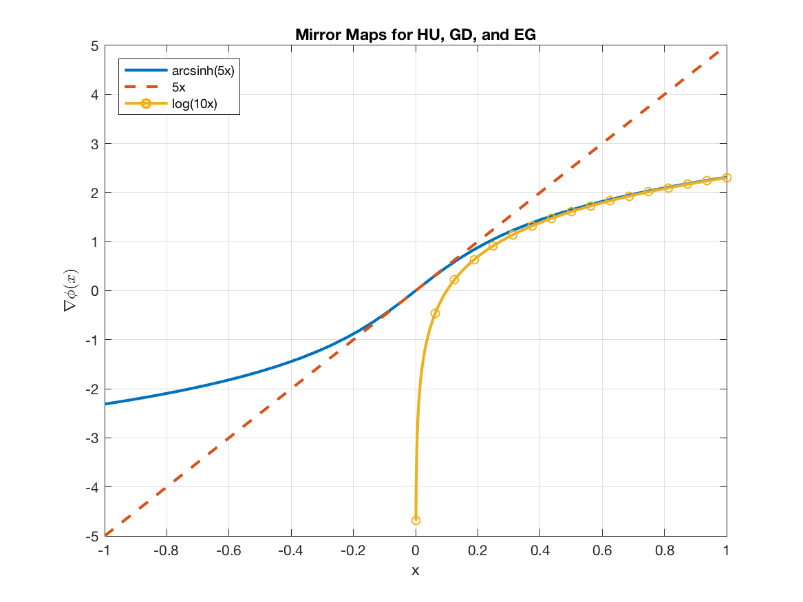
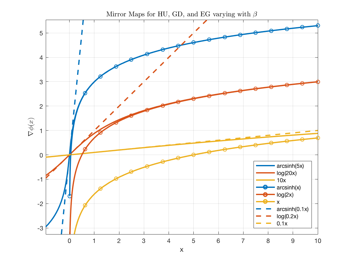
Figure 1: Left:Classical and new divergences. Center: scalar versions of mirror maps used in $\operatorname{HU}(\beta=\frac{1}{5})$, GD, and EG Algorithms depicted in blue, red, and yellow respectively. EG is only defined for positive values of $x$. Right: $\beta$ is varied between $0.1,1,$ and $10$ and is similarly depicted along with its linear and logarithmic limits.

From a mirror descent perspective of mirror descent (see Sec. A), it makes sense to look at the mirror map, the gradient of the $\phi$ which defines the dual space where additive gradient updates take place. Weights are mapped into the dual space via the mirror map $\nabla\phi:\mathbb{R}^{d}\rightarrow\mathbb{R}^{d}$ and mapped back into the primal space via $\nabla\phi^{*}$. Gradient-Descent (GD) can be framed as mirror descent using the squared euclidean norm potential while Exponentiated-Gradient (EG) amounts to mirror descent using the entropy potential. The Hypentropy Update (HU) uses the mirror map $\nabla\phi_{\beta}$. As can be seen from Figure 1, for sufficiently large weights, the hypentropy mirror map behaves like $\log(x)$, namely, the EG mirror map. In contrast, $\operatorname{arcsinh}(x/\beta)$ is linear for small weights, and thus behave like GD. Large values of $\beta$ correspond to a slower transition from the linear regime to the logarithmic regime of the mirror map.

The regret analysis of GD and EG depend on geometric properties of the divergence related to the $2$-norm and $1$-norm respectively. Given this connection, it is useful to analyze the properties of hypentropy with respect to both the $1$-norm and $2$-norm. Recall that a function $f$ is $\alpha$-strongly convex with respect to a norm $\|\cdot\|$ on ${\cal K}$ if,

$$\forall\mathbf{x},\mathbf{y}\in{\cal K},f(\mathbf{x})-f(\mathbf{y})-\nabla f(\mathbf{y})(\mathbf{x}-\mathbf{y})\geq\frac{\alpha}{2}\|\mathbf{x}-\mathbf{y}\|^{2}.$$

For convenience, we use the following second order characterization of strong-convexity from Thm.  3 in Yu (2013).

Lemma 3.2.

Let ${\cal K}$ be a convex subset of some finite vector space ${\cal X}$. A twice differentiable function $f:{\cal K}\rightarrow\mathbb{R}$ is $\alpha$-strongly convex with respect to a norm $\|\cdot\|$ iff

$$\inf_{\mathbf{x}\in{\cal K},\mathbf{y}\in{\cal X}:\|\mathbf{y}\|=1}\mathbf{y}^{\top}\,\nabla^{2}\phi(\mathbf{x})\,\mathbf{y}\geq\alpha~{}.$$

We next prove elementary properties of $\phi_{\beta}$.

Lemma 3.3.

The function $\phi_{\beta}$ is $(1+\beta)^{-1}$-strongly-convex over $B_{2}$ w.r.t the $2$-norm.

Proof 3.4.

To prove the first part, note that from (1) we get that the Hessian is the diagonal matrix,

$$\nabla^{2}\phi_{\beta}(\mathbf{x})=\operatorname{diag}\Big{[}\tfrac{1}{\sqrt{x_{1}^{2}+\beta^{2}}},\ldots\tfrac{1}{\sqrt{x_{d}^{2}+\beta^{2}}}\Big{]}$$

Strong convexity follows from the diagonal structure of the Hessian, whose smallest eigenvalue is

$$\frac{1}{\sqrt{x^{2}+\beta^{2}}}\geq\frac{1}{\sqrt{1+\beta^{2}}}\geq\frac{1}{1+\beta}~{}.$$

Lemma 3.5.

The function $\phi_{\beta}$ is $(1+\beta d)^{-1}$-strongly-convex over $B_{1}$ w.r.t. the $1$-norm.

Proof 3.6.

We work with the characterization provided in Lemma 3.2,

$$\inf_{\mathbf{x}\in B_{1},\|\mathbf{y}\|_{1}=1} \mathbf{y}^{\top}\nabla^{2}\phi(\mathbf{x})\mathbf{y}~{}=\inf_{\mathbf{x}\in B_{1},\|\mathbf{y}\|_{1}=1}\sum_{i=1}^{d}\frac{y_{i}^{2}}{\sqrt{\beta^{2}+x_{i}^{2}}} \big{[}\mbox{Equation}~{}\eqref{second_deriv:eq}\big{]}$$

$$=\inf_{\mathbf{x}\in B_{1},\|\mathbf{y}\|_{1}=1}\frac{1}{\sum_{i=1}^{d}\sqrt{\beta^{2}+x_{i}^{2}}}\,\bigg{(}\sum_{i=1}^{d}\frac{y_{i}^{2}}{\sqrt{\beta^{2}+x_{i}^{2}}}\bigg{)}\,\bigg{(}\sum_{i=1}^{d}\sqrt{\beta^{2}+x_{i}^{2}}\bigg{)}$$

$$\geq\inf_{\mathbf{x}\in B_{1},\|\mathbf{y}\|_{1}=1}\frac{1}{\sum_{i=1}^{d}\sqrt{\beta^{2}+x_{i}^{2}}}\bigg{(}\sum_{i=1}^{d}\sqrt{y_{i}^{2}}\bigg{)}^{2} \big{[}\mbox{Cauchy- Schwarz}\big{]}$$

$$=\inf_{\mathbf{x}\in B_{1},\|\mathbf{y}\|_{1}=1}\frac{1}{\sum_{i=1}^{d}\sqrt{\beta^{2}+x_{i}^{2}}}\|\mathbf{y}\|^{2}_{1}\geq\frac{1}{\sum_{i=1}^{d}(\beta+|x_{i}|)}\geq\frac{1}{1+\beta d}~{}.$$

We next introduce a generalized notion of diameter and use it to prove properties of $\phi_{\beta}$.

Definition 3.7.

The diameter of a convex set ${\cal K}$ with respect to $\phi$ is, $\mathrm{diam}_{\phi}({\cal K})\stackrel{{\scriptstyle\text{def}}}{{=}}\sup_{\mathbf{x}\in{\cal K}}D_{\phi}(\mathbf{x}\;\|\;\boldsymbol{0})~{}.$

Whenever implied by the context we omit the potential $\phi$ from the diameter. Before we consider two specific diameters below, we bound the diameter in general as follows,

$$D^{\beta}_{\phi}(\mathbf{x}\;\|\;\boldsymbol{0}) =\phi_{\beta}(\mathbf{x})-\phi_{\beta}(\boldsymbol{0})$$

$$=\sum_{i=1}^{d}\Big{(}x_{i}\operatorname{arcsinh}({x_{i}}/{\beta})-\sqrt{x^{2}_{i}+\beta^{2}}\Big{)}+\beta d$$

$$\leq\sum_{i=1}^{d}x_{i}\operatorname{arcsinh}({x_{i}}/{\beta})$$

$$=\sum_{i=1}^{d}|x_{i}|\log\left(\frac{1}{\beta}\left(\sqrt{x^{2}_{i}+\beta^{2}}+|x_{i}|\right)\right)$$

Thus, without loss of generality, we can assume that $\mathbf{x}$ lies in the positive orthant. We next bound the diameter of $B_{2}$ as follows,

$$\mathrm{diam}(B_{2}) \leq\sum_{i=1}^{d}x_{i}\log{\left(\frac{1}{\beta}\left(\sqrt{x^{2}_{i}+\beta^{2}}+x_{i}\right)\right)}$$

$$\leq\sum_{i=1}^{d}x_{i}\log{\Big{(}1+\frac{2x_{i}}{\beta}\Big{)}}$$

$$\leq\sum_{i=1}^{d}\frac{2x^{2}_{i}}{\beta}=\frac{2\|\mathbf{x}\|^{2}_{2}}{\beta}\leq\frac{2}{\beta}~{}.$$ (2)

For $\beta\leq 1$ and $\mathbf{x}\in B_{1}$ it holds that, ${\sqrt{x^{2}_{i}+\beta^{2}}+x_{i}}\leq\sqrt{2}+1$. Hence, for $\beta\leq 1$, we have

$$\mathrm{diam}(B_{1}) \leq\sum_{i=1}^{d}x_{i}\log{\Big{(}\frac{1+\sqrt{2}}{\beta}\Big{)}}=\|\mathbf{x}\|_{1}\log{\Big{(}\frac{1+\sqrt{2}}{\beta}\Big{)}}\leq\log{\Big{(}\frac{3}{\beta}\Big{)}}~{}.$$ (3)

3.1 HU algorithm

We next describe an OCO algorithm over a convex domain ${\cal K}\subseteq\mathbb{R}^{d}$. [ht] KwByby $\eta>0,\beta>0$, convex domain ${\cal K}\subseteq\mathbb{R}^{d}$ Initialize weight vector $\mathbf{w}^{1}=\boldsymbol{0}$  $i=1$ $T$ (a) Predict $\mathbf{w}^{t}$     (b) Incur loss $\ell_{t}(\mathbf{w}_{t})$     (c) Calculate $\mathbf{g}^{t}=\nabla\ell_{t}(\mathbf{w}^{t})$   Update: $\mathbf{w}^{t+\frac{1}{2}}=\beta\sinh{\Big{(}\operatorname{arcsinh}{\Big{(}\frac{\mathbf{w}^{t}}{\beta}\Big{)}}-\eta\mathbf{g}^{t}}\Big{)}$  Project onto ${\cal K}$: $\mathbf{w}^{t+1}=\displaystyle\operatorname*{arg\,min}_{\mathbf{v}\in{\cal K}}D^{\beta}_{\phi}(\mathbf{v}\;\|\;\mathbf{w}^{t+\frac{1}{2}})$ Hypentropy Update (HU)

$\operatorname{HU}$ is an instance of OMD with divergence $D^{\beta}_{\phi}(\cdot\!\;\|\;\!\cdot)$. We provide a simple regret analysis that follows directly from the geometric properties derived above. The following theorem allows us to bound the regret of an OMD algorithm in terms of the diameter and strong convexity.

Theorem 3.8.

Assume that $R:{\cal K}\rightarrow\mathbb{R}$ is $\mu$-strongly convex in respect to a norm $\|\cdot\|$ whose dual norm is $\|\cdot\|_{*}$. Assume that the diameter of ${\cal K}$ is bounded, $\mathrm{diam}_{R}({\cal K})\leq D$. Last, assume that $\forall{}t,\\ |\mathbf{g}^{t}\|_{*}\leq{}G$, then the regret boound of $\operatorname{HU}$ and learning rate $\eta=\sqrt{{2\mu D}/({TG^{2}})}$ satisfies

$$\operatorname{\mathcal{R}}_{T}\leq 2\sqrt{2\mu^{-1}DTG^{2}}~{}.$$

This follows from the more general Theorem A.1. We next provide regret bounds for $\operatorname{HU}$ over $B_{1}$ and $B_{2}$.

Theorem 3.9 (Additive Regret).

Let $\mathbf{w}\in B_{2}$ and assume that for all $t$, $\|\mathbf{g}_{t}\|_{2}\leq G_{2}$. Setting $\beta\geq 1$,

$$\eta=\frac{1}{G_{2}}\sqrt{\frac{1}{\beta(\beta+1)T}}~{},~{}\mbox{ yields }~{}~{}\operatorname{\mathcal{R}}_{T}(\operatorname{HU})\leq 4G_{2}\sqrt{T}~{}.$$

Proof 3.10.

Applying Lemma 3.3 and the diameter bounds from (2) to Theorem 3.8 yields,

$$\operatorname{\mathcal{R}}_{T}\leq 2\sqrt{2(1+\frac{1}{\beta})TG^{2}_{2}}\leq 4G_{2}\sqrt{T}~{}.$$

The final inequality follows from the condition that $\beta\geq 1$.

Theorem 3.11 (Multiplicative Regret).

Let $\mathbf{w}\in B_{1}$ and assume that for all $t$, $\|\mathbf{g}_{t}\|_{\infty}\leq G_{\infty}$. Setting for $\beta\leq 1$

$$\eta=\frac{1}{G_{\infty}}\sqrt{\frac{\log{\big{(}\tfrac{3}{\beta}\big{)}}}{2T(1+\beta d)}}~{},~{}\mbox{ yields }~{}~{}\operatorname{\mathcal{R}}_{T}(\operatorname{HU})\leq 3G_{\infty}\sqrt{T(1+\beta d)\log{(\tfrac{3}{\beta})}}~{}.$$

Proof 3.12.

Applying Lemma 3.5 and the diameter bounds from (3) to Theorem 3.8 yields,

$$\operatorname{\mathcal{R}}_{T}\leq 2G_{\infty}\sqrt{2T(1+\beta d)\log{\big{(}\tfrac{3}{\beta}\big{)}}}\leq 3G_{\infty}\sqrt{T(1+\beta d)\log{(\tfrac{3}{\beta})}}~{}.$$

4 Spectral Hyperbolic Divergence

In this section, the focus is on using hypentropy as a spectral regularization function. We show that the matrix version of $\operatorname{HU}$ is strongly convex with respect to the trace norm. Our proof technique of strong convexity is a roundabout for the matrix potential. The proof works by showing that the conjugate potential function is smooth with respect to the spectral norm (the dual of the trace norm). The duality of smoothness and strong convexity is then used to show strong convexity.

4.1 Matrix Functions

We are concerned with potential functions that act on the singular values of a matrix. For an even scalar function, $f:\mathbb{R}\rightarrow\mathbb{R}^{+}$, consider the trace function,

$$F(\mathbf{X})=(f\circ\sigma)(\mathbf{X})=\sum_{i=1}^{d}f(\sigma_{i})=\operatorname{Tr}\left(f\left(\sqrt{\mathbf{X}^{\top}\mathbf{X}}\right)\right)~{},$$ (4)

where we overload the notation for $f$ and denote $f(\mathbf{v})=\sum_{i=1}^{d}f(v_{i})$. For $\mathbf{X}\in\SS^{d}$ we use

$$F(\mathbf{X})=(f\circ\lambda)(\mathbf{X})=\operatorname{Tr}(f(\mathbf{X}))~{}.$$ (5)

Here $f(\mathbf{X})$ represents the standard lifting of a scalar function to a square matrix, where $f$ acts on the vector of eigenvalues, namely,

$$\mathbf{X}=\mathbf{U}\operatorname{diag}\left[\lambda(\mathbf{X})\right]\mathbf{U}^{\top}\quad\Rightarrow\quad f(\mathbf{X})=\mathbf{U}\operatorname{diag}\left[f(\lambda(\mathbf{X}))\right]\mathbf{U}^{\top}~{}.$$

We also use the gradient of a trace-function in our analysis. The following result from Thm. 14 in Kakade et al. (2009) shows how to compute a gradient using a singular value decomposition.

Theorem 4.1.

Let $\mathbf{X}\in\mathbb{R}^{m\times n}$ and $F:\mathbb{R}^{m\times n}\rightarrow\mathbb{R}^{+}$ be defined as above, then

$$\nabla F(\mathbf{X})=f^{\prime}(\mathbf{X})~{}.$$

We also make use of the Fenchel conjugate functions. Consider a convex function $f:{\cal X}\rightarrow\mathbb{R}$ defined on a finite vector space ${\cal X}$ endowed with an inner product $\langle\cdot,\cdot\rangle$. The conjugate of $f$ is defined as follows.

Definition 4.2.

The conjugate $f^{*}:{\cal X}\rightarrow\mathbb{R}$ of a convex function $f:{\cal X}\rightarrow\mathbb{R}$ is

$$f^{*}(\mathbf{z})=\sup_{\mathbf{x}\in{\cal X}}\langle\mathbf{x},\mathbf{z}\rangle-f(\mathbf{x})~{}.$$

In this section, we use the space of matrices (either $\mathbb{R}^{m\times n}$ or $\SS^{d})$ with the inner product $\langle\mathbf{X},\mathbf{Y}\rangle=\operatorname{Tr}(\mathbf{X}^{\top}\mathbf{Y})$. Thus, the dual space of ${\cal X}$ is ${\cal X}$ itself and $f^{*}$ is defined over ${\cal X}$.

We need to relate the conjugate of a trace function to that of a scalar function. This is achieved by the following result, restated from Thm. 12 Kakade et al. (2009). The theorem implies that the conjugate of a singular-values function is the singular-values function lifted from the conjugate of the scalar function.

Theorem 4.3.

Let $F=(f\circ\sigma)$ be defined as in (4), then $F^{*}=(f^{*}\circ\sigma)$.

4.2 Duality of Strong Convexity and Smoothness

Recall that a function $f$ is $L$-smooth with respect to a norm $\|\cdot\|$ on ${\cal K}$ if,

$$\forall\mathbf{x},\mathbf{y}\in{\cal K},~{}~{}f(\mathbf{x})-f(\mathbf{y})-\nabla f(\mathbf{y})(\mathbf{x}-\mathbf{y})\leq\frac{L}{2}\|\mathbf{x}-\mathbf{y}\|^{2}~{}.$$

For convenience, we use the following second order characterization of smoothness which is an analogue of Lemma 3.2.

Lemma 4.4.

A twice differentiable function $f:{\cal X}\rightarrow\mathbb{R}$ is locally $L$-smooth with respect to $\|\cdot\|$ at $\mathbf{x}$ iff

$$\sup_{\mathbf{y}\in{\cal X}:\|\mathbf{y}\|=1}\mathbf{y}^{\top}\nabla^{2}\phi(\mathbf{x})\,\mathbf{y}\leq L~{}.$$

Strong convexity and smoothness are dual notions in the sense that $f$ is $\alpha$-strongly convex with respect to a norm $\|\cdot\|$ iff its Fenchel conjugate $f^{*}$ is ${\alpha}^{-1}$-smooth with respect to the dual norm $\|\cdot\|_{*}$.

For the matrix variant of hypentropy we find it easier to show smoothness of the conjugate rather than strong convexity directly. Unfortunately, as we see in the sequel, the conjugate function is not smooth everywhere. Therefore, we would need a local variant of the duality of strong convexity and smoothness. In the context of mirror descent with mirror map $\nabla\phi$, we show that $\phi$ is strongly convex over ${\cal K}$ if $\phi^{*}$ is locally smooth at all points within the image of the mirror map. Formally, we have the following lemma. In the following we use the standard notation for image of vector functions, $\nabla f(S)=\{y|\nabla f(x)=y,x\in S\}$,

Lemma 4.5 (Local duality of smoothness and strong convexity).

Let ${\cal K}\subseteq\mathbb{R}^{d}$ be an open convex set and $\|\cdot\|$ be a norm with dual norm $\|\cdot\|_{*}$. Let $\phi:\mathbb{R}^{d}\rightarrow\mathbb{R}$ be twice differentiable, closed and convex function. Suppose the Fenchel conjugate $\phi^{*}:\mathbb{R}^{d}\rightarrow\mathbb{R}$ is locally $L$ smooth with respect to $\|\cdot\|_{*}$ at all points in ${\cal C}=\nabla\phi({\cal K})$. Then, $\phi$ is $\frac{1}{L}$ strongly convex with respect to $\|\cdot\|$ over ${\cal K}$.

Proof 4.6.

It suffices to show that for any $\mathbf{x}\in{\cal K}$, $\phi$ is locally $\frac{1}{L}$-strongly convex with respect to $\|\cdot\|$ at $\mathbf{x}$ if $\phi^{*}$ is locally $L$-smooth at $\mathbf{x}^{*}=\nabla\phi(\mathbf{x})$ with respect to $\|\cdot\|_{*}$.

From local smoothness at $\mathbf{x}^{*}$, we have for any $\mathbf{y}\in{\cal K}$,

$$f(\mathbf{y})=\frac{1}{2}\mathbf{y}^{\top}\nabla^{2}\phi^{*}(\mathbf{x}^{*})\mathbf{y}\leq\frac{L}{2}\|\mathbf{y}\|^{2}_{*}~{}.$$

Taking the dual, which is order reversing, we have for any $\mathbf{z}\in{\cal K}$,

$$f^{*}(\mathbf{z})=\frac{1}{2}\mathbf{z}^{\top}[\nabla^{2}\phi^{*}(\mathbf{x}^{*})]^{-1}\mathbf{z}\geq\frac{1}{2L}\|\mathbf{z}\|^{2}~{}.$$ (6)

Since $\nabla\phi^{*}=(\nabla\phi)^{-1}$, then from the inverse function theorem, we have that

$$\nabla^{2}\phi^{*}(\mathbf{x}^{*})=[\nabla^{2}\phi(\mathbf{x})]^{-1}~{}.$$

Using the above equality in (6), we have for any $\mathbf{z}\in{\cal K}$,

$$\frac{1}{2}\mathbf{z}^{\top}\nabla^{2}\phi(\mathbf{x})\mathbf{z}\geq\frac{1}{2L}\|\mathbf{z}\|^{2}~{}.$$

4.3 Strong Convexity of Spectral Hypentropy

We now analyze the strong convexity of the spectral hypentropy . The spectral function $\Phi_{\beta}(\mathbf{X})$ is defined for $\mathbf{X}\in\mathbb{R}^{m\times n}$ by (4) and for $\mathbf{X}\in\SS^{d}$ by (5) replacing $f$ with $\phi_{\beta}$. The main theorem of this subsection is as follows.

Theorem 4.7.

The trace function $\Phi_{\beta}:\mathbb{R}^{m\times n}\rightarrow\mathbb{R}$ is $(2(\tau+\beta\min\{m,n\}))^{-1}$-strongly convex with respect to the trace norm over $B_{\scriptscriptstyle\mathrm{Tr}\!\!}\left(\tau\right)$.

We denote the $d$-dimensional symmetric matrices of trace-ball with maximal radius $\tau$ by

$$\mathbb{B}_{\scriptscriptstyle\mathrm{Tr}\!\!}\left(\tau\right)=\{\mathbf{X}\in\SS^{d}:\|\mathbf{X}\|_{1}\leq\tau\}~{}.$$

We prove the above theorem by first proving the lemma below for matrices in $\mathbb{B}_{\scriptscriptstyle\mathrm{Tr}\!\!}\left(\tau\right)$. We then extend it to arbitrary matrices using a symmetrization argument, using a technique similar to Juditsky and Nemirovski (2008); Warmuth (2007); Hazan et al. (2012).

Definition 4.8.

Let ${\cal K}\subseteq\mathbb{B}_{\scriptscriptstyle\mathrm{Tr}\!\!}\left(\tau\right)$ be a subset of matrices and ${\cal X}\subseteq\SS^{d}$ be a vector space containing ${\cal K}$ such that $\forall\mathbf{X}\in{\cal X},\operatorname{rank}(\mathbf{X})\leq r$ and $\nabla\Phi_{\beta}(\mathbf{X})\in{\cal X}$.

This abstraction will be useful in translating strong convexity of arbitrary matrices to the symmetric case. The bound on the rank is essential to give a modulus of strong convexity result that depends only on $\min\{m,n\}$ rather than $m+n$. The final property is necessary for the low rank structure to be preserved after a primal-dual mapping.

Lemma 4.9.

The trace function $\Phi_{\beta}$ is $(2(\tau+\beta r))^{-1}$-strongly convex w.r.t the trace norm over ${\cal K}$.

To prove the symmetric variant, we show that $\Phi^{*}_{\beta}$ is smooth with respect to the spectral norm, which is the dual norm of the trace norm. The result then follows directly from Lemma 4.5.

From Theorem 4.3, $\Phi_{\beta}$ has Fenchel conjugate

$$\Phi^{*}_{\beta}(\mathbf{X})=\operatorname{Tr}(\phi^{*}_{\beta}(\mathbf{X}))~{}.$$

Since the derivative of the conjugate of a function is the inverse of the derivative of the function, we have

$$\frac{d\phi^{*}_{\beta}}{dx}=\left(\frac{d\phi_{\beta}}{dx}\right)^{-1}=\beta\sinh(x)~{}.$$

The indefinite integral of the above yields that up to a constant, $\phi^{*}_{\beta}(x)=\beta\cosh(x)$. Clearly, $\Phi_{\beta}$ is not smooth everywhere. Nonetheless, we do have smoothness over $\nabla\Phi_{\beta}(\mathbb{B}_{\scriptscriptstyle\mathrm{Tr}\!\!}\left(\tau\right))$. Before proving this property, we introduce a clever technical lemma of Juditsky and Nemirovski (2008) that allows us to reduce the spectral smoothness for matrices to smoothness of functions in the vector-case.

Lemma 4.10.

Let $f:\mathbb{R}\rightarrow\mathbb{R}$ be a function and $c\in\mathbb{R}_{+}$ such that that for $a\geq b$,

$$\frac{f^{\prime}(a)-f^{\prime}(b)}{a-b}\leq\frac{c(f^{\prime\prime}(a)+f^{\prime\prime}(b))}{2}~{}.$$ (7)

Let $F:\SS^{d}\rightarrow\mathbb{R}$ be a function defined by $F(\mathbf{X})=\operatorname{Tr}(f(\mathbf{X}))$. Then, the second directional derivative of $F$ is bounded for any $\mathbf{H}\in\SS^{d}$ as follows,

$$D^{2}{F(\mathbf{X})}\left[\mathbf{H},\mathbf{H}\right]\leq c\operatorname{Tr}(\mathbf{H}f^{\prime\prime}(\mathbf{X})\mathbf{H})~{}.$$

We are now prepared to analyze the smoothness of $\Phi^{*}_{\beta}$.

Lemma 4.11 (Local Smoothness).

The trace function $\Phi^{*}_{\beta}$ is locally $2(\tau+\beta r)$-smooth with respect to the spectral norm for all matrices in $\nabla\Phi_{\beta}({\cal K})$.

Proof 4.12.

To prove local smoothness, we use the second order conditions from Lemma 4.4. This requires us to upper bound the second directional derivatives for all directions corresponding to matrices of unit spectral norm. We consider the matrix

$$\mathbf{X}=\nabla\Phi(\mathbf{Y})=\phi_{\beta}^{\prime}(\mathbf{Y})=\operatorname{arcsinh}\left(\frac{\mathbf{Y}}{\beta}\right)~{}.$$

Note that $(\phi^{*}_{\beta})^{\prime\prime}(x)=\beta\cosh(x)$ is positive and convex. Therefore, by the mean value theorem, there exists $c\in[a,b]$ for which,

$$\frac{(\phi^{*}_{\beta})^{\prime}(b)-(\phi^{*}_{\beta})^{\prime}(a)}{b-a}=(\phi^{*}_{\beta})^{\prime\prime}(c)\leq\max\left\{\phi^{*}_{\beta})^{\prime\prime}(a)\,,\,(\phi^{*}_{\beta})^{\prime\prime}(b)\right\}\leq(\phi^{*}_{\beta})^{\prime\prime}(a)+(\phi^{*}_{\beta})^{\prime\prime}(b)~{}.$$

We note that by Definition 4.8, $\nabla\Phi_{\beta}({\cal X})\subseteq{\cal X}$, so we can restrict ourselves to the vector space ${\cal X}$. Therefore, applying Lemma 4.10, we have

$$\sup_{\mathbf{H}\in{\cal X}:\|\mathbf{H}\|_{\infty}\leq 1}D^{2}{\Phi_{\beta}^{*}(\mathbf{X})}\left[\mathbf{H},\mathbf{H}\right] \leq\sup_{\mathbf{H}\in{\cal X}:\|\mathbf{H}\|_{\infty}\leq 1}2\operatorname{Tr}\left(\mathbf{H}(\phi^{*}_{\beta})^{\prime\prime}(\mathbf{X})\,\mathbf{H}\right)$$

$$=\sup_{\mathbf{H}\in{\cal X}:\|\mathbf{H}\|_{\infty}\leq 1}2\operatorname{Tr}\left(\mathbf{H}^{2}(\phi^{*}_{\beta})^{\prime\prime}(\mathbf{X})\right) [\mbox{Commutativity of trace}]$$

$$\leq\sup_{\mathbf{H}\in{\cal X}:\|\mathbf{H}\|_{\infty}\leq 1}2\langle\sigma^{2}(\mathbf{H}),\sigma((\phi^{*}_{\beta})^{\prime\prime}(\mathbf{X}))\rangle [\mbox{von Neumann's trace inequality}]$$

where von Neumann’s trace inequality stands for, $\operatorname{Tr}(\mathbf{A}^{\top}\mathbf{B})\leq\langle\sigma(\mathbf{A}),\sigma(\mathbf{B})\rangle$. Now, since $\mathbf{H}\in{\cal X}$, we know $\operatorname{rank}(\mathbf{H})\leq r$, and so $\mathbf{H}$ can have at most $r$ nonzero singular values, yielding

$$\sup_{\mathbf{H}\in{\cal X}:\|\mathbf{H}\|_{\infty}\leq 1}D^{2}{\Phi_{\beta}^{*}(\mathbf{X})}\left[\mathbf{H},\mathbf{H}\right] \leq\sup_{\mathbf{H}\in{\cal X}:\|\mathbf{H}\|_{\infty}\leq 1}2\|\mathbf{H}^{2}\|_{\infty}\sum_{i=1}^{r}\sigma_{i}((\phi^{*}_{\beta})^{\prime\prime}(\mathbf{X}))$$

$$=2\sum_{i=1}^{r}(\phi^{*}_{\beta})^{\prime\prime}(\phi_{\beta}^{\prime}(\sigma_{i}(\mathbf{Y})))~{}.$$

Now, note that

$$(\phi_{\beta}^{*})^{\prime\prime}(\phi_{\beta}^{\prime}(x))=\beta\cosh\left(\operatorname{arcsinh}\left({x}/{\beta}\right)\right)=\sqrt{\beta^{2}+x^{2}}\leq\beta+|x|~{}.$$

It then follows that

$$\sum_{i=1}^{r}(\phi^{*}_{\beta})^{\prime\prime}(\phi_{\beta}^{\prime}(\sigma_{i}(\mathbf{Y})))\leq\beta r+\|\mathbf{Y}\|_{1}\leq\tau+\beta r~{}.$$

Therefore, the second directional derivative in bounded by $2(\tau+\beta r)$ as desired.

Proof 4.13 (Theorem 4.7).

We introduce the symmetrization operator $S:\mathbb{R}^{m\times n}\rightarrow\SS^{m+n}$ which is a linear function that takes a matrix to a symmetric matrix,

$$S(\mathbf{X})=\begin{bmatrix}0&\mathbf{X}\\ \mathbf{X}^{\top}&0\end{bmatrix}~{}.$$

The eigenvalues of $S(\mathbf{X})$ are exactly one copy of singular values and one copy of negative singular values of $\mathbf{X}$. Therefore, we have

$$\Phi_{\beta}(\mathbf{X})=\sum_{i=1}^{\min\{m,n\}}\phi_{\beta}(\sigma_{i}(\mathbf{X}))=\frac{1}{2}{\Phi_{\beta}(S(\mathbf{X}))}~{}.$$

Technically, for the above to hold true, we should shift $\phi_{\beta}$ such that its $0$ is at $0$. Since a constant shift does not affect diameter or convexity properties so this is not an issue.

Let $\mu$ be the modulus of strong convexity in the symmetrized space. We bound $\Phi_{\beta}(\mathbf{X})$ from below as follows,

$$2\Phi_{\beta}(\mathbf{X}) =\Phi_{\beta}(S(\mathbf{X}))$$

$$\geq\Phi_{\beta}(S(\mathbf{Y}))+\langle\nabla\Phi_{\beta}(S(\mathbf{Y})),S(\mathbf{X})-S(\mathbf{Y})\rangle+\frac{\mu}{2}\|S(\mathbf{X})-S(\mathbf{Y})\|^{2}_{1}$$

$$=\Phi_{\beta}(S(\mathbf{Y}))+\langle\nabla\Phi_{\beta}(S(\mathbf{Y})),S(\mathbf{X}-\mathbf{Y})\rangle+\frac{\mu}{2}\|S(\mathbf{X}-\mathbf{Y})\|^{2}_{1}$$

$$=2\Phi_{\beta}(\mathbf{Y})+2\langle\nabla\Phi_{\beta}(\mathbf{Y}),\mathbf{X}-\mathbf{Y}\rangle+2\mu\|\mathbf{X}-\mathbf{Y}\|^{2}_{1}~{}.$$

Therefore, the modulus of strong convexity over asymmetric matrices is $2\mu$.

Note that ${\cal K}=\{S(\mathbf{X}):\mathbf{X}\in B_{\scriptscriptstyle\mathrm{Tr}\!\!}\left(2\tau\right)\}$ satisfies the properties listed in Definition 4.8, with $r=2\min\{m,n\}$. In particular, we have a vector space ${\cal X}=\{S(\mathbf{X}):\mathbf{X}\in\mathbb{R}^{m\times n}\}$ containing symmetric matrices of rank at most $2\min\{m,n\}$. Furthermore, for any $\mathbf{X}\in{\cal X}$, $\mathbf{X}=S(\mathbf{Y})$ for some $\mathbf{Y}\in\mathbb{R}^{m\times n}$ and thus,

$$\nabla\Phi_{\beta}(\mathbf{X})=\nabla\Phi_{\beta}(S(\mathbf{Y}))=S(\nabla\Phi_{\beta}(\mathbf{Y}))\in{\cal X}~{}.$$

It follows from Theorem 4.9 that $\mu\geq(2(2\tau+2\beta\min\{m,n\}))^{-1}$, and so the strong convexity is at most $2\mu\geq(2(\tau+\beta\min\{m,n\}))^{-1}$ as desired.

4.4 SHU algorithm

We next describe, the Spectral Hypentropy Update ($\operatorname{SHU}$), an OCO algorithm over a convex domain of matrices ${\cal K}\subseteq\mathbb{R}^{m\times n}$.

[ht] KwByby $\eta>0,\beta>0$, convex domain of matrices ${\cal K}\subseteq\mathbb{R}^{m\times n}$ Initialize weight matrix $\mathbf{W}^{1}=\boldsymbol{0}$  $i=1$ $T$ (a) Predict $\mathbf{W}^{t}$     (b) Incur loss $\ell_{t}(\mathbf{W}_{t})$     (c) Calculate $\mathbf{G}^{t}=\nabla\ell_{t}(\mathbf{W}^{t})$   Update: $\mathbf{W}^{t+\frac{1}{2}}=\beta\sinh{\Big{(}\operatorname{arcsinh}{\Big{(}\frac{\mathbf{W}^{t}}{\beta}\Big{)}}-\eta\mathbf{G}^{t}}\Big{)}$  Project onto ${\cal K}$: $\mathbf{W}^{t+1}=\displaystyle\operatorname*{arg\,min}_{\mathbf{V}\in{\cal K}}D^{\beta}_{\Phi}(\mathbf{V}\;\|\;\mathbf{W}^{t+\frac{1}{2}})$ Spectral Hypentropy Update (SHU)

The pseudocode of $\operatorname{SHU}$ is provided in Algorithm 4.4. The update step of SHU requires a spectral decomposition. We define $f(\mathbf{A})=\mathbf{U}f(\operatorname{diag}\left[\sigma(\mathbf{A})\right])\mathbf{V}^{\top}$ where $\mathbf{A}=\mathbf{U}\operatorname{diag}(\sigma(\mathbf{A}))\mathbf{V}^{\top}$ is the singular value decomposition of $\mathbf{A}$. We use this definition twice, once with $f=\operatorname{arcsinh}$, and after subtracting the gradient with $f=\sinh$. We prove the following regret bound for $\operatorname{SHU}$.

Theorem 4.14.

Let $\mathbf{W}\in B_{\scriptscriptstyle\mathrm{Tr}\!\!}\left(\tau\right)\subseteq\mathbb{R}^{m\times n}$ and let $\|\mathbf{G}^{t}\|_{\infty}\leq G_{\infty}$ be a spectral norm bound on the gradients. For $\gamma=\frac{\beta}{\tau}\leq 1$, setting,

$$\eta=\frac{1}{2G_{\infty}}\sqrt{\frac{\log{\big{(}\tfrac{3}{\gamma}\big{)}}}{T(1+\gamma\min\{m,n\})}}~{},~{}\mbox{ yields }~{}~{}\operatorname{\mathcal{R}}_{T}(\operatorname{SHU})\leq 4\tau G_{\infty}\sqrt{T(1+\gamma\min\{m,n\})\log{(\tfrac{3}{\gamma})}}~{}.$$

Proof 4.15.

Like for $\operatorname{HU}$, we use the general OMD analysis. It suffices to find an upper bound on $\mathrm{diam}_{\Phi_{\beta}}(B_{\scriptscriptstyle\mathrm{Tr}\!\!}\left(\tau\right))$ and a strong convexity bound.

Applying (3) on the vector singular values, we have

$$\mathrm{diam}_{\Phi_{\beta}}(B_{\scriptscriptstyle\mathrm{Tr}\!\!}\left(\tau\right))\leq\tau\log\left(\frac{3\tau}{\beta}\right)~{},$$

where $\beta\leq\tau$. Furthermore, from Theorem 4.7, we can see that $\Phi_{\beta}$ is $(2(\tau+\beta\min\{m,n\}))^{-1}$ strongly convex with respect to the trace-norm over $B_{\scriptscriptstyle\mathrm{Tr}\!\!}\left(\tau\right)$. Letting $\gamma=\frac{\beta}{\tau}$, the result follows from Theorem 3.8.

5 Experimental Results

Next, we experiment with HU in the context of empirical risk minimization (ERM). In the experiments, $\mathbf{g}_{t}$ stands for a stochastic estimate of the gradient of the empirical loss. Thus, we can convert the regret analysis to convergence in expectation Cesa-Bianchi et al. (2004).

Effective Learning Rate

For small value $w$, $\sinh(w)\approx w\approx\operatorname{arcsinh}(w)$. As a result, near $0$ the update in $\operatorname{HU}$ is morally the additive update, $w_{i}^{t+1}=w_{i}^{t}-\beta\eta g^{t}_{i}$. The product $\beta\eta$ can be viewed as the de facto learning rate of the gradient descent portion of the interpolation. As such, we define the effective learning rate to be $\beta\eta$. In the sequel, fixing the effective learning rate while changing $\beta$ is a fruitful lens for comparing $\operatorname{HU}$ to with $\operatorname{GD}$.

5.1 Logistic Regression

In this experiment we use the $\operatorname{HU}$ algorithm to optimize a logit model. The ambient dimension $d$ is chosen to be $500$. A weight $\mathbf{w}$ is drawn uniformly at random from $[-1,1]^{d}$. The features are from $\{0,1\}^{d}$ and distributed according to the power law, $\Pr[x_{i}=1]={1}/{5\sqrt{i}}$. The label associated with an example $\mathbf{x}_{t}$ is set to $y_{t}=\operatorname{sign}(\langle\mathbf{w},\mathbf{x}_{t}\rangle)$ with with probability $0.9$ and otherwise flipped.

The algorithms are trained with log-loss using batches of size $10$. Stochastic gradient descent and the $p$-norm algorithm Gentile (2003) are used for comparison. As can be seen in Fig. 2, the $p$-norm algorithm performs significantly worse than HU for a large set of values of $\beta$, while SGD performs comparably. As expected, for large value of $\beta$, SGD and HU are indistinguishable.

 

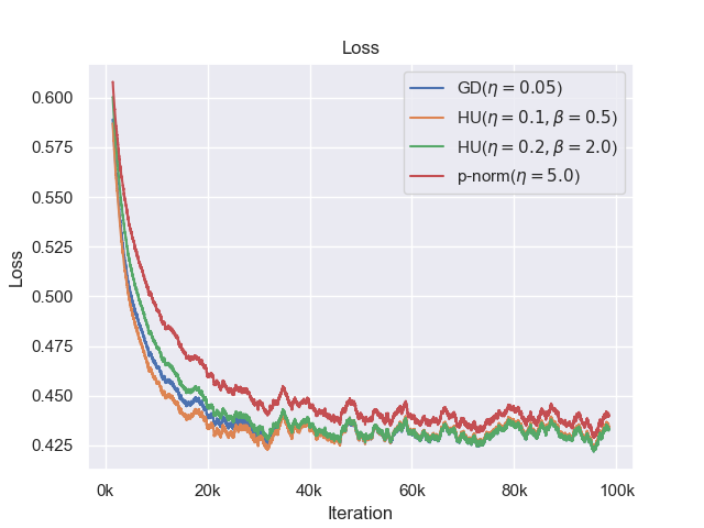
Figure 2: Comparison of accuracy and loss of GD, $p$-norm, and $\operatorname{HU}$ on binary logistic regression.

In the next experiment we use the same logit model with ambient dimension $d$ chosen to be $10,000$. We generate weights, $\mathbf{w}\in\mathbb{R}^{d}$, with sparsity (fraction of zero weights) $s\in\{0,0.9\}$. The nonzero weights are chosen uniformly at random from $[-1,1]$. We run the algorithms for 20,000 iterations. Rather than fixing $\eta$, we fix $\eta^{\prime}={\eta}/{\sqrt{1+\beta^{2}}}$. This way, as $\beta\to\infty$, $\operatorname{HU}(\eta^{\prime},\beta)$ behaves like $\operatorname{GD}(\eta)$ while for small $\beta$, the update is roughly $\operatorname{EG\pm}(\eta)$. We let $\beta_{\operatorname{EG}}={\|\mathbf{w}^{\star}\|_{1}}/{d}$. As discussed in Appendix B, this choice of $\beta$ is similar to running $\operatorname{EG\pm}$ with an $1$-norm bound of $\|\mathbf{w}^{\star}\|_{1}$. We then choose $\eta^{\prime}=0.1$ and $\beta\in\{0.5,1,2,4,8\}\times\beta_{\operatorname{EG}}$. In Fig. 3, we show the interpolation between $\operatorname{GD}$ and $\operatorname{EG\pm}$. The larger $\beta$ is, the closer the progress of HU resembles that of $\operatorname{GD}$. Intermediate values of $\beta$ have progress in between the $\operatorname{EG\pm}$ and $\operatorname{GD}$.

 

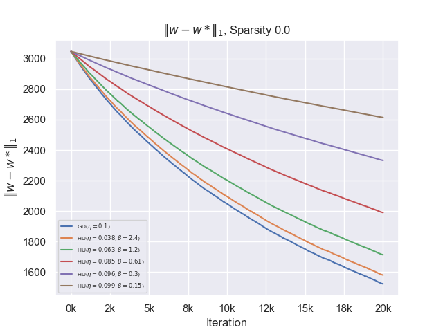
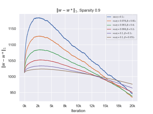
Figure 3: Value of $\|\mathbf{w}^{t}-\mathbf{w}^{\star}\|_{1}$ in dense and sparse settings with $\eta^{\prime}=0.1$ and $\beta\in\{0.5,1,2,4,8\}\times\beta_{\operatorname{EG}}$.

5.2 Multiclass Logistic Regression

In this experiment we use $\operatorname{SHU}$ to optimize a multiclass logistic model. We generated 200,000 examples in $\mathbb{R}^{25}$. We set the number of classes to $k=15$. Labels are generated using a rank $5$ matrix $\mathbf{W}\in\mathbb{R}^{k\times d}$. An example $\mathbf{x}\in\mathbb{R}^{d}$ was labeled according to the prediction rule,

$$y=\operatorname*{arg\,max}_{i\in[k]}\{(\mathbf{W}\mathbf{x})_{i}\}~{}.$$

With probability $5.0\%$ the label was flipped to a different one at random. The matrix $\mathbf{W}$ and each example $\mathbf{x}_{i}$ features are determined in a joint process to make the problem poorly conditioned for optimization. Features of each example are first drawn from a standard normal. Weights of $\mathbf{W}$ are sampled from a standard normal distribution for the first $r$ features and are set to $0$ for the remaining $d-r$ features. After labels are computed, features are perturbed by Gaussian noise with standard deviation $0.05$. The examples and weights are then scaled and rotated. Coordinate $i$ of the data is scaled by $s_{i}\propto i^{-1.1}$ where $\sum_{i=1}^{d}s_{i}=1$. Then a random rotation $\mathbf{R}$ is applied. The inverse of these transformation is applied to the weights. Therefore, from the original sample $\mathbf{X}_{0}\in\mathbb{R}^{n\times d}$ and weights $\mathbf{W}_{0}\in\mathbb{R}^{k\times d}$ the new sample and weights are set to be $\mathbf{X}=\mathbf{X}_{0}\mathbf{R}$ and $\mathbf{W}=\mathbf{W}_{0}\mathbf{R}^{-1}$, where $\mathbf{R}\in\mathbb{R}^{d\times d}$ is the scaling and rotation described above.

Since our ground truth weights are low rank, our goal is to find weights of approximately low rank with low classification error. To do this, we optimize a multiclass logistic regression loss with a trace-norm constraint. We compare $\operatorname{SHU}$, Schatten $p$-norm algorithm ($p$-norm algorithm applied to singular values) and gradient descent in the fully stochastic (single example) case. We report results for unconstrained optimization in Fig. 4 and trace-norm constrained optimization in Fig. 5. In these figures only the algorithms with lowest final loss after a grid search are depicted.

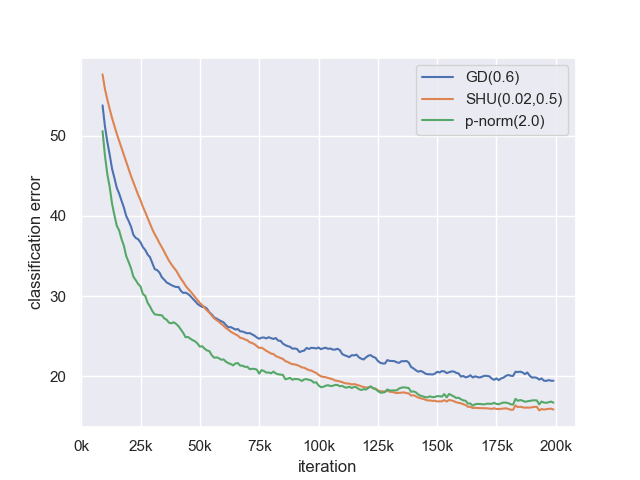
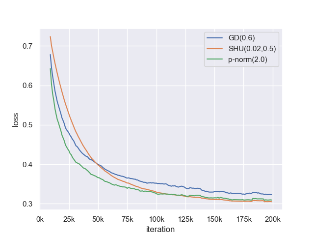
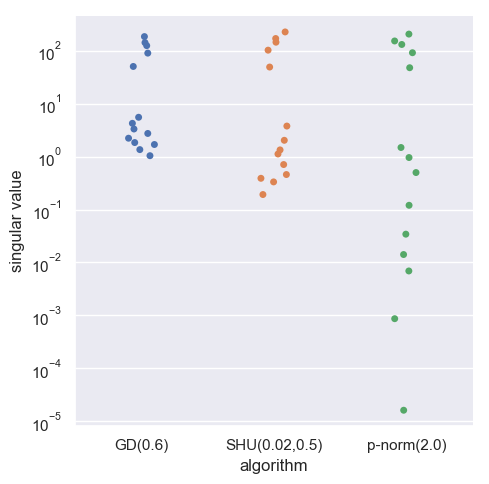
Figure 4: Unconstrained minimization of logistic loss.

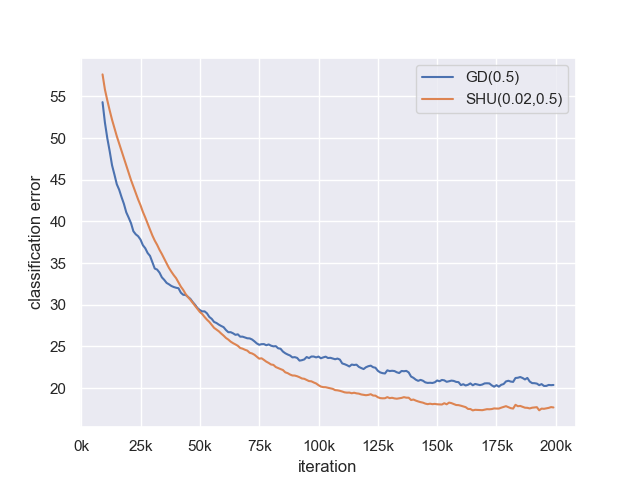
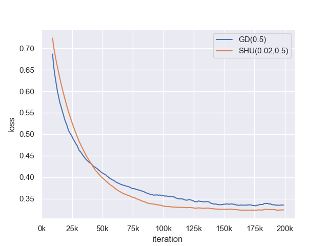
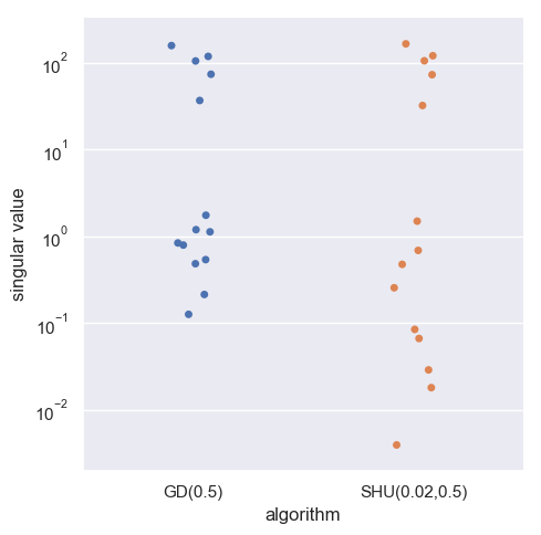
Figure 5: Minimization over the trace-norm ball of radius $500$. The $p$-norm algorithm is not included becaus ethe $p$-norm divergence does not have a closed form projection onto the $1$-ball.

Without projection, $\operatorname{SHU}$ results in the largest trace norm solution of norm $700$ whereas the $p$-norm algorithm and $\operatorname{GD}$ reach solutions with trace norm just above $600$. Nevertheless, $\operatorname{SHU}$ attains the lowest classification error and loss. Performance is noticeably better than gradient descent. Moreover, the spurious singular values are typically smaller than that of gradient descent. This pattern holds up in both settings.

With our new divergence, the $\operatorname{SHU}$ update looks exponential for large singular values and linear for small ones. In this sense, once gradients start accumulating in the directions that correspond to the actual signal, these directions can be exploited exponentially. On the other hand, the spurious directions are morally handled with gradient descent with an effective learning rate $\eta\beta$. Note that in our experiments, the $\operatorname{SHU}$ effective learning rate is smaller than the $\operatorname{GD}$ learning rate by an order of magnitude. This may explain the smaller magnitude in erroneous singular values. On the other hand, the $p$-norm algorithm not only increases the magnitude of large singular values, but also shrinks the magnitude of small singular values, resulting in solutions that are closer to being low-rank. To see this, note that the $p$-norm inverse mirror map has the form

$$f(\boldsymbol{\sigma})_{i}=\sigma_{i}^{p-1}/\|\boldsymbol{\sigma}\|^{p-2}_{p}$$

for $p=2\ln(k)\approx 5.4$. Therefore, there is a natural normalization which shrinks small singular values as good directions are exploited. Without projection, this does not happen with $\operatorname{SHU}$. Informally speaking, the following analogy applies to the three methods:

$\operatorname{GD}$:   The rich get richer!

$\operatorname{SHU}$:   The rich get much richer!!

$p$-norm:   The rich get richer and the poor get poorer, oy!

Adding trace norm projection reduces the magnitude of these singular values, but not to the level which the $p$-norm algorithm can achieve. Overall, it appears that $\operatorname{SHU}$ may be slightly more effective at reducing loss but the $p$-norm algorithm is more effective at producing low rank solutions.

5.3 Image Classification with Neural Networks.

Loss minimization for neural networks is known to be nonconvex, thus the regret bounds from this paper do not apply in this setting. Still, convex optimization algorithms, such as AdaGrad, work well practice for training neural networks. In this section, we use the unconstrained version of the HU to find the weights of a simple neural network for image classification using the popular CIFAR10 dataset Krizhevsky et al. . SGD was used for comparison. Outside of use of the HU algorithm, the design of the network and code are from the Tensorflow tutorial on convolutional networks for image classification. The network involves $2$ convolutional layers, max pooling, and $2$ fully connected layers, all using ReLU activations. The loss function is the cross entropy loss plus a $2$-norm regularization. For a complete description of the experimental setup see TFT ; Krizhevsky and Hinton (2009).

Empirically, SGD with learning rate $\eta$ tended to perform similarly in terms of training error to HU with equivalent effective learning rate $\beta\eta$ for a range of values of $\beta$. In order to compare to SGD with learning rate $\eta$, $\beta$ was varied and HU’s learning rate was set to be $\frac{\eta}{\beta}$ (in order to keep the effective learning rate invariant). As can be seen from Figure 6, the loss curves for a variety of values of $\beta$ are very similar for $\beta\eta=0.005$, although the smallest $\beta=0.1$ has slightly lower loss. In general, the final loss reached is similar for a fixed effective learning rate. In addition, there is a clear pattern indicating that shrinking $\beta$ results in sparser weights. This may warrant further investigation.

 

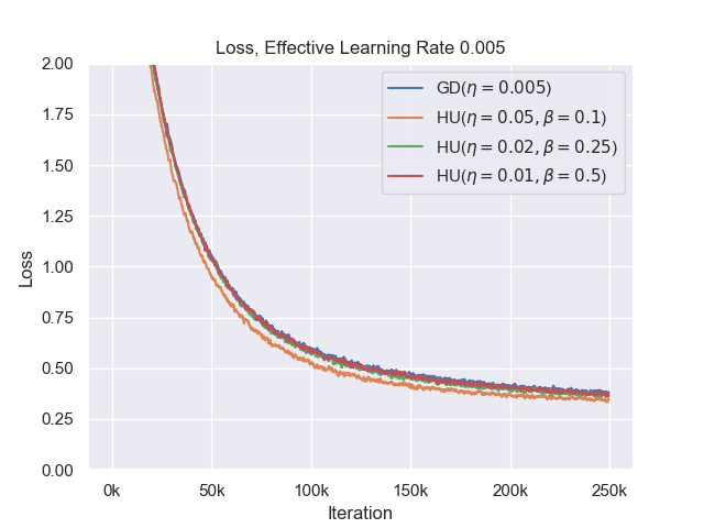
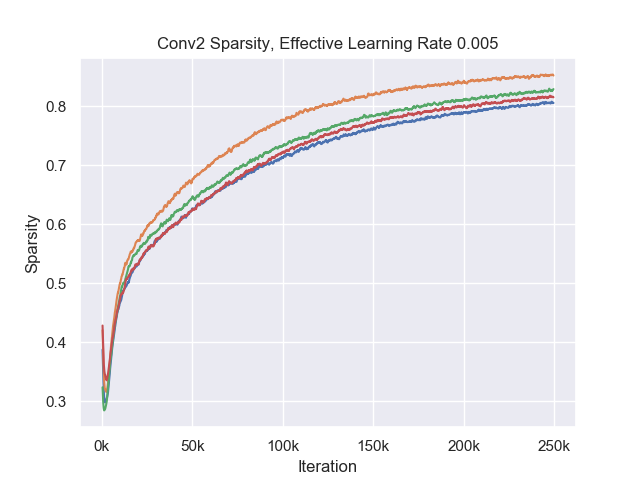
Figure 6: CIFAR10 loss and sparsity level. The effective learning rate was held constant at $0.005$ while $\beta$ is varied. Sparsity is displayed for the second convolutional layer conv2. The loss corresponds to the total loss, which includes regularization.

6 Discussion

We examined a new regularization for online learning which interpolates between multiplicative and additive updates through of a single parameter $\beta>0$. As $\beta\to\infty$, the algorithm approaches gradient descent while as $\beta\to\frac{1}{d}$ it behaves similarly to the multiplicative update. The spectral regularization provides a matrix analogue which is naturally applicable to rectangular matrices. An interesting open direction is to devise an self-tuning update for $\beta$ which is data dependent.

We thank Orestis Plevrakis for enlightening discussion.

Appendix A Online Mirrored Descent

[h] KwByby $\eta>0,\beta>0$, convex domain ${\cal K}\subseteq\mathbb{R}^{d}$ Let $\mathbf{y}_{1}$ be such that $\nabla R(\mathbf{y}_{1})=0$ and $\mathbf{w}^{1}=\operatorname*{arg\,min}_{\mathbf{w}\in{\cal K}}D_{R}(\mathbf{w}\;\|\;\mathbf{y}^{1})$  $i=1$ $T$ (a) Predict $\mathbf{w}^{t}$     (b) Incur loss $\ell_{t}(\mathbf{W}_{t})$     (c) Calculate $\mathbf{g}^{t}=\nabla\ell_{t}(\mathbf{w}^{t})$   Update: $\nabla R(\mathbf{y}^{t+1})=\nabla R(\mathbf{w}^{t})-\eta\mathbf{g}^{t}$  Project onto ${\cal K}$: $\mathbf{w}^{t+1}=\operatorname*{arg\,min}_{\mathbf{w}\in{\cal K}}D_{R}(\mathbf{w}\;\|\;\mathbf{y}^{t+1})$ Online Mirror Descent with potential function $R$

Online Mirror Descent (OMD) is an meta-algorithm for online convex optimization. The regularization function, $R$, is assumed to be strongly convex, smooth, and twice differentiable. Like GD, Mirror Descent is an iterative algorithm involving a simple gradient update. $R$ defines a mapping into a dual space where the updates occur, followed by an inverse mapping to the original space. This step may result in a vector outside of ${\cal K}$, so a projection is required. An alternative formulation where the regularization casts a trade-off between moving along the gradient direction and staying close to the current iterate is,

$$\mathbf{w}^{t+1} =\operatorname*{arg\,min}_{\mathbf{w}\in{\cal K}}\big{\{}\eta\langle\mathbf{g}^{t},\mathbf{w}\rangle+D_{R}(\mathbf{w}\;\|\;\mathbf{w}^{t})\big{\}}~{}.$$ (8)

For Algorithm A with the above assumptions, we have the following regret bound.

Theorem A.1 (OMD Regret).

Assume $R$ is $\mu$-strongly convex with respect to a norm $\|\cdot\|$ whose dual is $\|\cdot\|_{*}$, then running OMD with a fixed learning rate $\eta$ yields the following regret bound,

$$\operatorname{\mathcal{R}}_{T}\leq\frac{1}{\eta}\,{\sup_{\mathbf{w}\in{\cal K}}D_{R}(\mathbf{w}\;\|\;\mathbf{w}^{1})}+\frac{\eta}{2\mu}\sum_{t=1}^{T}\|\mathbf{g}^{t}\|^{2}_{*}~{}.$$

If we have a bound on the dual norm of a gradient, we can choose a learning rate which minimizes the upper bound, yielding Theorem 3.8. We next introduce two well known properties of Bregman divergences without proof. The first technical lemma is the Bregman divergence analogue of the law of cosines.

Lemma A.2 (Three-point Lemma).

For every three vectors $\mathbf{x},\mathbf{y},\mathbf{z}$,

$$D_{R}(\mathbf{x}\;\|\;\mathbf{z})=D_{R}(\mathbf{x}\;\|\;\mathbf{y})+D_{R}(\mathbf{y}\;\|\;\mathbf{z})-\langle\nabla R(\mathbf{z})-\nabla R(\mathbf{y}),\mathbf{x}-\mathbf{y}\rangle~{}.$$

The next lemma is an analogue of the Pythagorean theorem for Bregman projections.

Lemma A.3 (Generalized Pythagorean Theorem).

Let

$$\mathbf{x}^{\prime}=\Pi_{{\cal K},\phi}(\mathbf{x})=\operatorname*{arg\,min}_{\mathbf{y}\in{\cal K}}D_{R}(\mathbf{y}\;\|\;\mathbf{x})~{},$$

then

$$D_{R}(\mathbf{z}\;\|\;\mathbf{x})\geq D_{R}(\mathbf{z}\;\|\;\mathbf{x}^{\prime})+D_{R}(\mathbf{x}^{\prime}\;\|\;\mathbf{x})~{}.$$

Proof A.4 (Theorem A.1).

Let $\mathbf{w}^{*}=\operatorname*{arg\,min}_{\mathbf{w}\in{\cal K}}\sum_{t=1}^{T}\ell_{t}(\mathbf{w})$ be the best fixed predictor in hindsight, then

$$\ell_{t}(\mathbf{w}^{t})-\ell_{t}(\mathbf{w}^{*}) \leq\langle\mathbf{g}^{t},\mathbf{w}^{t}-\mathbf{w}^{*}\rangle [\mbox{Convexity}]$$

$$=\frac{1}{\eta}\langle\nabla R(\mathbf{w}^{t})-\nabla R(\mathbf{y}^{t+1}),\mathbf{w}^{t}-\mathbf{w}^{*}\rangle$$

$$=\frac{1}{\eta}\langle\nabla R(\mathbf{y}^{t+1})-\nabla R(\mathbf{w}^{t}),\mathbf{w}^{*}-\mathbf{w}^{t}\rangle$$

$$=\frac{1}{\eta}\big{(}D_{R}(\mathbf{w}^{*}\;\|\;\mathbf{w}^{t})+D_{R}(\mathbf{w}^{t}\;\|\;\mathbf{y}^{t+1})-D_{R}(\mathbf{w}^{*}\;\|\;\mathbf{y}^{t+1})\big{)} [\mbox{Lemma}~{}\ref{3pt:lemma}]$$

$$=\frac{1}{\eta}\big{(}D_{R}(\mathbf{w}^{*}\;\|\;\mathbf{w}^{t})+D_{R}(\mathbf{w}^{t}\;\|\;\mathbf{y}^{t+1})-D_{R}(\mathbf{w}^{*}\;\|\;\mathbf{w}^{t+1})-D_{R}(\mathbf{w}^{t+1}\;\|\;\mathbf{y}^{t+1})\big{)} [\mbox{Lemma}~{}\ref{pythog:lemma}]$$

$$=\frac{1}{\eta}\big{(}D_{R}(\mathbf{w}^{*}\;\|\;\mathbf{w}^{t})-D_{R}(\mathbf{w}^{*}\;\|\;\mathbf{w}^{t+1}))+\frac{1}{\eta}\big{(}D_{R}(\mathbf{w}^{t}\;\|\;\mathbf{y}^{t+1})-D_{R}(\mathbf{w}^{t+1}\;\|\;\mathbf{y}^{t+1})\big{)}~{}.$$

Note that the left hand side term telescopes when summing over $t$, yielding

$$\sum_{t=1}^{T}\ell_{t}(\mathbf{w}^{t})-\ell_{t}(\mathbf{w}^{*})\leq\frac{D_{R}(\mathbf{w}^{*}\;\|\;\mathbf{w}^{1})}{\eta}+\frac{1}{\eta}\sum_{t=1}^{T}\Big{(}D_{R}(\mathbf{w}^{t}\;\|\;\mathbf{y}^{t+1})-D_{R}(\mathbf{w}^{t+1}\;\|\;\mathbf{y}^{t+1})\Big{)}~{}.$$ (9)

If suffices to upper bound $D_{R}(\mathbf{w}^{t}\;\|\;\mathbf{y}^{t+1})-D_{R}(\mathbf{w}^{t+1}\;\|\;\mathbf{y}^{t+1})$. We start by substituting the definition of the Bregman divergence in $D_{R}$,

$$D_{R}(\mathbf{w}^{t}\;\|\;\mathbf{y}^{t+1}) -D_{R}(\mathbf{w}^{t+1}\;\|\;\mathbf{y}^{t+1})$$

$$=R(\mathbf{w}^{t})-R(\mathbf{w}^{t+1})-\langle\nabla R(\mathbf{y}^{t+1}),\mathbf{w}^{t}-\mathbf{w}^{t+1}\rangle$$

$$\leq\langle\nabla R(\mathbf{w}^{t}),\mathbf{w}^{t}-\mathbf{w}^{t+1}\rangle-\frac{\mu}{2}\|\mathbf{w}^{t}-\mathbf{w}^{t+1}\|^{2}-\langle\nabla R(\mathbf{y}^{t+1}),\mathbf{w}^{t}-\mathbf{w}^{t+1}\rangle [\mu\mbox{-strong convexity}]$$

$$=\langle\nabla R(\mathbf{w}^{t})-\nabla R(\mathbf{y}^{t+1}),\mathbf{w}^{t}-\mathbf{w}^{t+1}\rangle-\frac{\mu}{2}\|\mathbf{w}^{t}-\mathbf{w}^{t+1}\|^{2}$$

$$=\eta\,\langle\mathbf{g}^{t},\mathbf{w}^{t}-\mathbf{w}^{t+1}\rangle-\frac{\mu}{2}\|\mathbf{w}^{t}-\mathbf{w}^{t+1}\|^{2} [\mbox{Update rule}]$$

$$\leq\eta\,\|\mathbf{g}^{t}\|_{*}\,\|\mathbf{w}^{t}-\mathbf{w}^{t+1}\|-\frac{\mu}{2}\|\mathbf{w}^{t}-\mathbf{w}^{t+1}\|^{2} [\mbox{ Cauchy-Schwarz}]$$

$$\leq\frac{\eta^{2}\|\mathbf{g}^{t}\|^{2}_{*}}{2\mu}~{}.$$

The last step follows from maximizing the quadratic function in $\|\mathbf{w}^{t}-\mathbf{w}^{t+1}\|$. Using the above bound (9) completes the proof.

Appendix B Connections to EG$\pm$

The $\operatorname{EG\pm}$ algorithm Kivinen and Warmuth (1997) maintains two vectors $\mathbf{u}$ and $\mathbf{v}$ such that, $\mathbf{w}=\mathbf{u}-\mathbf{v}$. The two vectors are updated over $\mathbb{R}^{2d}_{+}$ using the $\operatorname{EG}$ algorithm. We consider here a variant where the $2d$ dimensional weights are normalized such that their sum is $\beta d$. Typically, we would have $\beta=\frac{1}{2d}$, so $(\mathbf{u},\mathbf{v})$ lie on a unit simplex.

[t] KwByby $\eta>0,\beta>0$ Initialize: $\mathbf{u}^{1}_{i}=\mathbf{v}^{1}_{i}=\frac{\beta}{2}$,  $\mkern 1.5mu\overline{\mkern-1.5mu\mathbf{g}\mkern-1.5mu}\mkern 1.5mu^{0}=\boldsymbol{0}$  $t=1$ $T$ (a) Predict $\mathbf{w}^{t}=\mathbf{u}^{t}-\mathbf{v}^{t}$     (b) Incur loss $\ell_{t}(\mathbf{w}_{t})$     (c) Calculate $\mkern 1.5mu\overline{\mkern-1.5mu\mathbf{g}\mkern-1.5mu}\mkern 1.5mu^{t}=\mkern 1.5mu\overline{\mkern-1.5mu\mathbf{g}\mkern-1.5mu}\mkern 1.5mu^{t-1}+\nabla\ell_{t}(\mathbf{w}^{t})$   Update: $u^{t+\frac{1}{2}}_{i}=u^{t}_{i}\exp(-\eta g^{t}_{i})$    and    $v^{t+\frac{1}{2}}_{i}=v^{t}_{i}\exp(\eta g^{t}_{i})$  Normalize weights: $(\mathbf{u}^{t+1},\mathbf{v}^{t+1})={\beta d}\,\Bigg{(}{\sum_{i=1}^{d}u^{t+\frac{1}{2}}_{i}+v^{t+\frac{1}{2}}_{i}}\Bigg{)}^{-1}\!\!(\mathbf{u}^{t+\frac{1}{2}},\mathbf{v}^{t+\frac{1}{2}})$ $\operatorname{EG\pm}$

We now show that the $\operatorname{EG\pm}$ algorithm can be viewed as an adaptive variant of $\operatorname{HU}$ with the update,

$$\mathbf{y}^{t+1}=(\nabla\phi_{\beta_{t}})^{-1}(\nabla\phi_{\beta_{t-1}}(\mathbf{w}^{t})-\eta\mathbf{g}^{t})~{}.$$ (10)

The weight, $\mathbf{w}^{t+1}$ is then hypentropy projection of $\mathbf{y}^{t+1}$ onto the contraint set. In this adaptive update, $\nabla\phi_{\beta_{t-1}}$ is used to map into the dual space where a gradient update occurs. Afterwards, $(\nabla\phi)^{-1}_{\beta_{t}}$ maps back to the primal. When used in an OCO setting over the norm-$1$ ball, $\beta_{t}$ can always be chosen to be sufficiently small such that projection step is voided. $\operatorname{EG\pm}$ fits into this algorithmic paradigm with a specific choice of $\beta_{t}$ that avoids hypentropy projection. In the setting of OCO over the norm-$1$ ball of radius $\beta d$, we have the following result.

Theorem B.1.

$\operatorname{EG\pm}$ with learning rate $\eta$ is equivalent to the adaptive $\operatorname{HU}$ algorithm described in (10) with the same learning rate and $\beta_{t}={\beta d}\left({\sum_{i=1}^{d}\cosh(\eta\mkern 1.5mu\overline{\mkern-1.5mu\mathbf{g}\mkern-1.5mu}\mkern 1.5mu^{t}_{i})}\right)^{-1}$, where $\mkern 1.5mu\overline{\mkern-1.5mu\mathbf{g}\mkern-1.5mu}\mkern 1.5mu^{t}=\sum_{s=1}^{t}\mathbf{g}^{t}$.

Proof B.2.

We start with some analysis of $\operatorname{EG\pm}$. We have $u^{t+1}_{i}\propto\exp(-\eta\mkern 1.5mu\overline{\mkern-1.5mu\mathbf{g}\mkern-1.5mu}\mkern 1.5mu^{t}_{i})$ and similarly $v^{t+1}_{i}\propto\exp(-\eta\mkern 1.5mu\overline{\mkern-1.5mu\mathbf{g}\mkern-1.5mu}\mkern 1.5mu^{t}_{i})$. Normalizing the two such that $\|(\mathbf{u}^{t+1},\mathbf{v}^{t+1})\|_{1}=\beta d$ yields the normalization factor,

$$\frac{\beta d}{\sum_{i=1}^{d}\exp(-\eta\mkern 1.5mu\overline{\mkern-1.5mu\mathbf{g}\mkern-1.5mu}\mkern 1.5mu^{t}_{i})+\exp(\eta\mkern 1.5mu\overline{\mkern-1.5mu\mathbf{g}\mkern-1.5mu}\mkern 1.5mu^{t}_{i})}=\frac{2\beta d}{\sum_{i=1}^{d}\cosh(\eta\mkern 1.5mu\overline{\mkern-1.5mu\mathbf{g}\mkern-1.5mu}\mkern 1.5mu^{t}_{i})}$$

Putting the above all together, we get

$$w^{t+1}_{i}=u^{t+1}-v^{t+1} =\frac{2\beta d}{\sum_{i=1}^{d}\cosh(\eta\mkern 1.5mu\overline{\mkern-1.5mu\mathbf{g}\mkern-1.5mu}\mkern 1.5mu^{t}_{i})}\big{(}\exp(-\eta\mkern 1.5mu\overline{\mkern-1.5mu\mathbf{g}\mkern-1.5mu}\mkern 1.5mu^{t}_{i})-\exp(\eta\mkern 1.5mu\overline{\mkern-1.5mu\mathbf{g}\mkern-1.5mu}\mkern 1.5mu^{t}_{i})\big{)}$$

$$=\frac{\beta d\sinh(-\eta\mkern 1.5mu\overline{\mkern-1.5mu\mathbf{g}\mkern-1.5mu}\mkern 1.5mu^{t}_{i})}{\sum_{i=1}^{d}\cosh(\eta\mkern 1.5mu\overline{\mkern-1.5mu\mathbf{g}\mkern-1.5mu}\mkern 1.5mu^{t}_{i})}$$ (11)

$$=\beta_{t}\sinh(-\eta\mkern 1.5mu\overline{\mkern-1.5mu\mathbf{g}\mkern-1.5mu}\mkern 1.5mu^{t}_{i})~{}.$$

Therefore, we have $\mathbf{w}^{t+1}=\nabla\phi^{-1}_{\beta_{t}}(-\eta\mkern 1.5mu\overline{\mkern-1.5mu\mathbf{g}\mkern-1.5mu}\mkern 1.5mu^{t})$. We can now show that the adaptive $\operatorname{HU}$ algorithm described in (10) results in the same weights. We prove this property by induction on $t$. The base case follows because we initialize $\mathbf{w}^{0}=0$ in $\operatorname{HU}$. Now we assume that $\mathbf{w}^{t}=\phi^{-1}_{\beta_{t-1}}(-\eta\mkern 1.5mu\overline{\mkern-1.5mu\mathbf{g}\mkern-1.5mu}\mkern 1.5mu^{t-1})$. Applying the hypentropy update, we have

$$\mathbf{y}^{t+1}=\nabla\phi_{\beta_{t}}^{-1}(\nabla\phi_{\beta_{t-1}}(\phi^{-1}_{\beta_{t-1}}(-\eta\mkern 1.5mu\overline{\mkern-1.5mu\mathbf{g}\mkern-1.5mu}\mkern 1.5mu^{t-1}))-\eta\mathbf{g}^{t})=\nabla\phi_{\beta_{t}}^{-1}(-\eta\mkern 1.5mu\overline{\mkern-1.5mu\mathbf{g}\mkern-1.5mu}\mkern 1.5mu^{t-1}-\eta\mathbf{g}^{t})=\nabla\phi^{-1}_{\beta_{t}}(-\eta\mkern 1.5mu\overline{\mkern-1.5mu\mathbf{g}\mkern-1.5mu}\mkern 1.5mu^{t})~{}.$$

Now note that since $\forall x\in\mathbb{R},|\sinh(x)|\leq\cosh(x)$, projection never takes place, so $\mathbf{w}^{t+1}=\mathbf{y}^{t+1}$.

We also find it useful to consider these updates without normalization or projection. Without any constraint, the regularization parameter $\beta$ does need to change.

Theorem B.3.

Running $\operatorname{HU}$ with a learning rate $\eta$ and a regularization parameter $\beta$ without projection is equivalent to running $\operatorname{EG\pm}$ without normalization.

Proof B.4.

Note that in $\operatorname{EG\pm}$ without normalization we get,

$$u^{t+1}_{i}v^{t+1}_{i}=u^{t}_{i}\exp(-\eta g^{t}_{i})v^{t}_{i}\exp(\eta g^{t}_{i})=u^{t}_{i}v^{t}_{i}~{}.$$

Therefore, $u^{t}_{i}v^{t}_{i}$ remains fixed and due to the initialization $\forall i,u^{0}_{i}v^{0}_{i}=\frac{\beta^{2}}{4}$. This inverse relationship between $\mathbf{u}$ and $\mathbf{v}$ can be used to find a simple closed form solution for $\mathbf{w}$ by solving a quadratic equation. In particular, we know $u>0$, so we have

$$w=u-v=u-\dfrac{\beta^{2}}{4u}~{}\Rightarrow~{}u=\dfrac{w+\sqrt{w^{2}+\beta^{2}}}{2}~{}.$$

The resulting final update is

$$w^{t+1}_{i} =\dfrac{\sqrt{(w^{t}_{i})^{2}+\beta^{2}}+w^{t}_{i}}{2}\exp(-\eta g^{t}_{i})-\dfrac{\sqrt{(w^{t}_{i})^{2}+\beta^{2}}-w^{t}_{i}}{2}\exp(\eta g^{t}_{i})$$

$$=\sqrt{(w^{t}_{i})^{2}+\beta^{2}}\dfrac{\exp(-\eta g^{t}_{i})-\exp(\eta g^{t}_{i})}{2}+w^{t}_{i}\dfrac{\exp(-\eta g^{t}_{i})+\exp(\eta g^{t}_{i})}{2}$$

$$=\sinh(-\eta g^{t}_{i})\sqrt{(w^{t}_{i})^{2}+\beta^{2}}+\cosh(-\eta g^{t}_{i})w^{t}_{i}~{}.$$

Now we consider HU algorithm with the same parameters,

$$\mathbf{w}^{t+1} =\nabla\phi_{\beta}^{-1}(\nabla\phi_{\beta}(\mathbf{w}^{t})-\eta\mathbf{g}^{t}) \big{[}\mbox{Algorithm~{}\ref{hu:algorithm} update}\big{]}$$

$$~{}~{}~{}\Rightarrow w^{t+1}_{i} =\beta\sinh\Big{(}\operatorname{arcsinh}\Big{(}\frac{w^{t}_{i}}{\beta}\Big{)}-\eta g^{t}_{i}\Big{)}$$

$$=\beta\Big{[}\sinh\Big{(}\operatorname{arcsinh}\Big{(}\frac{w^{t}_{i}}{\beta}\Big{)}\Big{)}\cosh(-\eta g^{t}_{i})+\cosh\Big{(}\operatorname{arcsinh}\Big{(}\frac{w^{t}_{i}}{\beta}\Big{)}\Big{)}\sinh(-\eta g^{t}_{i})\Big{]}$$

$$=\sinh(-\eta g^{t}_{i})\sqrt{(w^{t}_{i})^{2}+\beta^{2}}+\cosh(-\eta g^{t}_{i})w^{t}_{i}~{}.$$

Thus indeed the two updates with the conditions stated in the theorem are equivalent.

Discussion

While, we can represent $\operatorname{EG\pm}$ as an adaptive variant of $\operatorname{HU}$, we still would like to understand how $\operatorname{HU}$ with a fixed $\beta$ relates to $\operatorname{EG\pm}$. A brief look into $\beta_{t}$ provides some intuition that the two still should be similar updates. Note that for small $\eta$, $\cosh(\eta\mkern 1.5mu\overline{\mkern-1.5mu\mathbf{g}\mkern-1.5mu}\mkern 1.5mu^{t}_{i})=1+O(\eta^{2})$ and $\beta_{t}\approx\beta$. In this regime, a fixed $\beta$ should result in a similar update. The relation to $\operatorname{EG\pm}$ also motivates the choice of $\beta\approx\tfrac{\|\mathbf{w}^{\star}\|}{d}$ as this provides the right scale for $\operatorname{EG\pm}$. Another takeaway from TheoremB.1 is that the $\operatorname{EG\pm}$ algorithm viewed without doubling has an update that looks very much like RFTL. For simplicity, let $\beta=\tfrac{1}{d}$. We see from (11) that the weights follow $\mathbf{w}^{t}=\nabla\phi^{*}(-\eta\mkern 1.5mu\overline{\mkern-1.5mu\mathbf{g}\mkern-1.5mu}\mkern 1.5mu^{t})$ where $\phi^{*}(\mathbf{x})=\log(\sum_{i=1}^{d}\cosh(x_{i}))$.

References

- (1) Advanced convolutional neural networks. https://goo.gl/8vmt1B.
- Arora and Kale (2007) S. Arora and S. Kale. A combinatorial, primal-dual approach to semidefinite programs. In Proc. 39th Symposium on Theory Of Computing, pages 227–236, 2007.
- Arora et al. (2012) S. Arora, E. Hazan, and S. Kale. The multiplicative weights update method: a meta-algorithm and applications. Theory of Computing, 8(1):121–164, 2012.
- Cesa-Bianchi and Lugosi (2006) N. Cesa-Bianchi and G. Lugosi. Prediction, learning, and games. Cambridge university press, 2006.
- Cesa-Bianchi et al. (2004) N. Cesa-Bianchi, A. Conconi, and C. Gentile. On the generalization ability of on-line learning algorithms. IEEE Transactions on Information Theory, 50(9):2050–2057, 2004.
- Duchi et al. (2011) J. Duchi, E. Hazan, and Y. Singer. Adaptive subgradient methods for online learning and stochastic optimization. Journal of Machine Learning Research, 12:2121–2159, 2011.
- Gentile (2003) C. Gentile. The robustness of the p-norm algorithms. Machine Learning, 53(3):265–299, 2003.
- Grove et al. (2001) A.J. Grove, N. Littlestone, and D. Schuurmans. General convergence results for linear discriminant updates. Machine Learning, 43(3):173–210, 2001.
- Hazan (2016) E. Hazan. Introduction to online convex optimization. Foundations and Trends in Optimization, 2(3-4):157–325, 2016.
- Hazan et al. (2012) E. Hazan, S. Kale, and S. Shalev-Shwartz. Near-optimal algorithms for online matrix prediction. In Conference on Learning Theory, pages 38–1, 2012.
- Juditsky and Nemirovski (2008) A. Juditsky and A.S. Nemirovski. Large deviations of vector-valued martingales in 2-smooth normed spaces. arXiv:0809.0813, 2008.
- Kakade et al. (2012) Sham M Kakade, Shai Shalev-Shwartz, and Ambuj Tewari. Regularization techniques for learning with matrices. Journal of Machine Learning Research, 13:1865–1890, 2012.
- Kakade et al. (2009) S.M. Kakade, S. Shalev-Shwartz, and A. Tewari. Applications of strong convexity–strong smoothness duality to learning with matrices. arXiv:0910.0610, 2009.
- Kivinen and Warmuth (1997) J. Kivinen and M.K. Warmuth. Exponentiated gradient versus gradient descent for linear predictors. Information and Computation, 132(1):1–63, 1997.
- Krizhevsky and Hinton (2009) A. Krizhevsky and G. Hinton. Learning multiple layers of features from tiny images. Technical report, 2009.
- (16) A. Krizhevsky, V. Nair, and G. Hinton. CIFAR-10. URL https://goo.gl/xKwPJo.
- Shalev-Shwartz (2012) S. Shalev-Shwartz. Online learning and online convex optimization. Foundations and Trends in Machine Learning, 4(2):107–194, 2012.
- Tsuda et al. (2005) K. Tsuda, G. Rätsch, and M.K. Warmuth. Matrix exponentiated gradient updates for on-line learning and bregman projection. Journal of Machine Learning Research, 6:995–1018, 2005.
- (19) Manfred Warmuth. Personal communication (circa 2010).
- Warmuth (2007) M.K. Warmuth. Winnowing subspaces. In Proc. 24th International Conference on Machine Learning, pages 999–1006, 2007.
- Yu (2013) Yao-Liang Yu. The strong convexity of von neumann’s entropy, June 2013.