Asymptotic Consistency of $\alpha$-Rényi-Approximate Posteriors

Abstract

We study the asymptotic consistency properties of $\alpha$-Rényi approximate posteriors, a class of variational Bayesian methods that approximate an intractable Bayesian posterior with a member of a tractable family of distributions, the member chosen to minimize the $\alpha$-Rényi divergence from the true posterior. Unique to our work is that we consider settings with $\alpha>1$, resulting in approximations that upperbound the log-likelihood, and consequently have wider spread than traditional variational approaches that minimize the Kullback-Liebler (KL) divergence from the posterior. Our primary result identifies sufficient conditions under which consistency holds, centering around the existence of a ‘good’ sequence of distributions in the approximating family that possesses, among other properties, the right rate of convergence to a limit distribution. We further characterize the good sequence by demonstrating that a sequence of distributions that converges too quickly cannot be a good sequence. We also extend our analysis to the setting where $\alpha$ equals one, corresponding to the minimizer of the reverse KL divergence, and to models with local latent variables. We also illustrate the existence of good sequence with a number of examples. Our results complement a growing body of work focused on the frequentist properties of variational Bayesian methods.
Keywords: $\alpha$-Rényi divergence, Asymptotic consistency, Bayesian computation, Variational inference

1 Introduction

Bayesian statistics forms a powerful and flexible framework that allows practitioners to bring prior knowledge to statistical problems, and to coherently manage uncertainty resulting from finite and noisy datasets. A Bayesian represents the unknown state of the world with a possibly vector-valued parameter $\theta$, over which they place a prior probability $\pi(\theta)$, representing a priori beliefs they might have. $\theta$ can include global parameters shared across the entire dataset, as well as local variables specific to each observation. A likelihood $p(\mathbf{X}_{n}|\theta)$ then specifies a probability distribution over the observed dataset $\mathbf{X}_{n}$. Given observations $\mathbf{X}_{n}$, prior beliefs $\pi(\theta)$ are updated to a posterior distribution $\pi(\theta|\mathbf{X}_{n})$ calculated through Bayes’ rule.

While conceptually straightforward, computing $\pi(\theta|\mathbf{X}_{n})$ is intractable for many interesting and practical models, and the field of Bayesian computation is focused on developing scalable and accurate computational techniques to approximate the posterior distribution. Traditionally, much of this has involved Monte Carlo and Markov chain Monte Carlo techniques to construct sampling approximations to the posterior distribution. In recent years, developments from machine learning have sought to leverage tools from optimization to construct tractable posterior approximations. An early and still popular instance of this methodology is variational Bayes (VB) (Blei et al., 2017).

At a high level, the idea behind VB is to approximate the intractable posterior $\pi(\theta|\mathbf{X}_{n})$ with an element $q(\theta)$ of some simpler class of distributions $\mathcal{Q}$. Examples of $\mathcal{Q}$ include the family of Gaussian distributions, delta functions, or the family of factorized ‘mean-field’ distributions that discard correlations between components of $\theta$. The variational solution $q$ is the element of $\mathcal{Q}$ that is closest to $\pi(\theta|\mathbf{X}_{n})$, where closeness is measured in terms of the Kullback-Leibler (KL) divergence. Thus, $q$ is the solution to:

$$q(\theta)=\text{argmin}_{\tilde{q}\in\mathcal{Q}}\text{KL}(\tilde{q}(\theta)\|\pi(\theta|\mathbf{X}_{n})).$$ (1)

We term this as the KL-VB method. From the non-negativity of the KL divergence, we can view this as maximizing a lower-bound to the logarithm of the model evidence , $\log p(\mathbf{X}_{n})=\log\left(\int p(\mathbf{X}_{n},\theta)\mathrm{d}\theta\right)$. This lower-bound, called the variational lower-bound or evidence lower bound (ELBO) is defined as

$$\text{ELBO}(\tilde{q}(\theta))=\log p(\mathbf{X}_{n})-\text{KL}(\tilde{q}(\theta)\|p(\theta|\mathbf{X}_{n})).$$ (2)

Optimizing the two equations above with respect to $q$ does not involve either calculating expectations with respect to the intractable posterior $\pi(\theta|\mathbf{X}_{n})$, or evaluating the posterior normalization constant. As a consequence, a number of standard optimization algorithms can be used to select the best approximation $q(\theta)$ to the posterior distribution, examples including expectation-maximization (Neal and Hinton, 1998) and gradient-based (Kingma and Welling, 2014) methods. This has allowed the application of Bayesian methods to increasingly large datasets and high-dimensional settings. Despite their widespread popularity in the machine learning, and more recently, the statistics communities, it is only recently that variational Bayesian methods have been studied theoretically (Alquier and Ridgway, 2020; Chérief-Abdellatif and Alquier, 2018; Wang and Blei, 2018; Yang et al., 2020; Zhang and Gao, 2020).

1.1 Rényi Divergence Minimization

Despite its popularity, variational Bayes has a number of well-documented limitations. An important one is its tendency to produce approximations that underestimate the spread of the posterior distribution (Turner and Sahani, 2011; Li and Turner, 2016): in essence, the variational Bayes solution tends to match closely with the dominant mode of the posterior. This arises from the choice of the divergence measure $\text{KL}(q(\theta)\|\pi(\theta|\mathbf{X}_{n}))=\mathbb{E}_{q}[\log(q(\theta)/\pi(\theta|\mathbf{X}_{n}))]$, which does not penalize solutions where $q(\theta)$ is small while $\pi(\theta|\mathbf{X}_{n})$ is large. While many statistical applications only focus on the mode of the distribution, definite calculations of the variance and higher moments are critical in predictive and decision-making problems.

A natural solution is to consider different divergence measures than those used in variational Bayes. Expectation propagation (EP) (Minka, 2001a) was developed to minimize $\mathbb{E}_{p}[\log(p/q)]$ instead, though this requires an expectation with respect to the intractable posterior. Consequently, EP can only minimize an approximation of this objective.

More recently, Rényi’s $\alpha$-divergence (Van Erven and Harremos, 2014) has been used as a family of parametrized divergence measures for variational inference (Li and Turner, 2016; Dieng et al., 2017). The $\alpha$-Rényi divergence is defined as

$$D_{\alpha}\left(\pi(\theta|\mathbf{X}_{n})\|{q}(\theta)\right):=\frac{1}{\alpha-1}\log\int_{\Theta}{q}(\theta)\left(\frac{\pi(\theta|\mathbf{X}_{n})}{{q}(\theta)}\right)^{\alpha}d\theta.$$

The parameter $\alpha$ spans a number of divergence measures and, in particular, we note that as $\alpha\to 1$ we recover the EP objective $\text{KL}(\pi(\theta|\mathbf{X}_{n})\|q(\theta))$, we will call its minimizer $1-$Rényi approximate posterior. Settings of $\alpha>1$ are particularly interesting since, in contrast to VB which lower-bounds the log-likelihood of the data (2), one obtains tractable upper bounds. Precisely, using Jensen’s inequality,

$$p(\mathbf{X}_{n})^{\alpha} =\left(\int p(\theta,\mathbf{X}_{n})\leavevmode\nobreak\ \frac{q(\theta)}{q(\theta)}\leavevmode\nobreak\ d\theta\right)^{\alpha}\leq\mathbb{E}_{q}\left[\left(\frac{p(\theta,\mathbf{X}_{n})}{q(\theta)}\right)^{\alpha}\right].$$

Applying the logarithm function on either side,

$$\alpha\log p(\mathbf{X}_{n}) \leq\log\mathbb{E}_{q}\left[\left(\frac{\pi(\theta,\mathbf{X}_{n})}{q(\theta)}\right)^{\alpha}\right]$$ (3)

$$=\alpha\log p(\mathbf{X}_{n})+\log\mathbb{E}_{q}\left[\left(\frac{\pi(\theta|\mathbf{X}_{n})}{q(\theta)}\right)^{\alpha}\right]:=\mathcal{F}_{2}(q).$$ (4)

Observe that the second term in the expression for $\mathcal{F}_{2}(q)$ is just $(\alpha-1)D_{\alpha}(p(\theta|\mathbf{X}_{n})\|q(\theta))$. Like with the ELBO lower bound, evaluating this upper bound only involves expectations with respect to $q(\theta)$, and only requires evaluating $p(\theta,\mathbf{X}_{n})$, the unnormalized posterior distribution. Optimizing this upper bound over some class of distributions $\mathcal{Q}$, we obtain the $\alpha$-Rényi approximation. As noted before, standard variational Bayes, which optimizes a lower-bound, tends to produce approximating distributions that underestimate the posterior variance, resulting in predictions that are overconfident and ignore high-risk regions in the support of the posterior. We illustrate this in Figure 1 below that reproduces a result from Li and Turner (2016). The true posterior distribution is an anisotropic Gaussian distribution and the variational family consists of isotropic (or mean-field) Gaussian distributions. Standard KL-VB, represented by the curve $\alpha=0$, clearly fits the mode of the posterior, but completely underestimates the dominant eigen-direction. On the other hand, for large values of $\alpha$ (shown as $\alpha\to+\infty$), the $\alpha$-Rényi approximate posterior matches the mode and does a better job of capturing the spread of the posterior. The figure also presents results for the $\alpha=1$ and the $\alpha\to-\infty$ cases. As an aside, we observe that our parametrization of the Rényi divergence is different from Li and Turner (2016), where the upper-bounds considered in Li and Turner (2016) emerge as $\alpha\to-\infty$.

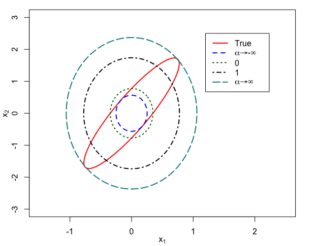
Figure 1: Isotropic variational $\alpha$-Rényi approximations to an anisotropic Gaussian, for different values of $\alpha$ (see also Li and Turner (2016)).

We note, furthermore, that in tasks such as model selection, the marginal likelihood of the data is of fundamental interest (Grosse et al., 2015), and the $\alpha$-Rényi upper bound provides an approximation that complements the VB lower bound. Recent developments in stochastic optimization have allowed the $\alpha$-Rényi objective to be optimized fairly easily; see Li and Turner (2016) and Dieng et al. (2017).

1.2 Large Sample Properties

Despite often state-of-the-art empirical results, variational methods still present a number of unanswered theoretical questions. This is particularly true for $\alpha$-Rényi divergence minimization which has empirically demonstrated very promising results for a number of applications (Li and Turner, 2016; Dieng et al., 2017). In recent work, Zhang and Gao (2020) have shown conditions under which $\alpha$-Rényi variational methods are consistent when $\alpha$ is less than one. Their results followed from a proof for the regular Kullback-Leibler variational algorithm, and thus only apply to situations when a lower-bound is optimized. As we mentioned before, the setting with $\alpha$ greater than $1$ is qualitatively different from both Kullback-Leibler and Rényi divergence with $\alpha<1$. This setting, which is also of considerable practical interest, is the focus of our paper and we address the question of asymptotic consistency of the approximate posterior distribution obtained by minimizing the Rényi divergence.

Asymptotic consistency (van der Vaart, 1998) is a basic frequentist requirement of any statistical method, guaranteeing that the ‘true’ parameter is recovered as the number of observations tends to infinity. Table 1 summarizes the current known results on consistency of VI and EP, and highlights the gap that this paper is intended to fill. We note that in this work, we are not analyzing the actual EP algorithm (Wainwright and Jordan, 2008), and are instead looking at the global minimizer of the ideal EP objective.

Methods	Papers
KL-VB	Wang and Blei (2018),Zhang and Gao (2020)
$\alpha$-Rényi ($\alpha<1$)	Zhang and Gao (2020)
$\alpha$-Rényi ($\alpha>1$)	This paper
$1$-Rényi ($\alpha\to 1$, global EP )	This paper

Table 1: Known results on the asymptotic consistency of variational methods.

As we will see, filling these gaps will require new developments. This follows from two complicating factors: 1) Rényi divergence with $\alpha>1$ upper-bounds the log-likelihood, and 2) this requires new analytical approaches involving expectations with respect to the intractable $\pi(\theta|\mathbf{X}_{n})$. We thus emphasize that the results in our paper are not a consequence of recent analysis in Wang and Blei (2018) and Zhang and Gao (2020) for the KL-VB, and our proofs differ substantially from theirs.

We establish our main result in Theorem 3.1 under mild regularity conditions. First, in Assumption 1 we assume that the prior distribution places positive mass in the neighborhood of the true parameter $\theta_{0}$, and that it is uniformly bounded. The former condition is a reasonable assumption to make - clearly, if the prior does not place any mass in the neighborhood of the true parameter (assuming one exists) then neither will the posterior. The uniform boundedness condition on the other hand is attendant to a loss of generality. In particular, we cannot assume certain heavy-tailed priors (such as Pareto) which might be important for some engineering applications. Second, we also make the mild assumption that the likelihood function is locally asymptotically normal (LAN) in Assumption 2. This is a standard assumption that holds for a variety of statistical/stochastic models. However, while the LAN assumption will be critical for establishing the asymptotic consistency results, it is unclear if it is necessary as well. We observe that Wang and Blei (2018) make a similar assumption in analyzing the consistency of KL-VB. We note that any model $P_{\theta}$ that is twice differentiable in the parameter $\theta$ satisfies the LAN condition (van der Vaart, 1998). Also critical to the consistency result are the properties of the variational family. Assumption 3 is a mild condition that insists on there existing Dirac delta distributions in an open neighborhood of the true parameter $\theta_{0}$. This is usually easy to verify: if the variational family consists of Gaussian distributions, for instance, then Dirac delta distributions are present at all points in the parameter space. Next, we assume that the variational family contains ‘good sequences’ that are constructed so as to converge at the same rate as the true posterior (in sequence with the sample size), with the first moment of an element in the sequence the maximum likelihood estimator of the parameter (at a given sample size). We also require the tails of the good sequence to bound the tails of the true posterior. We provide examples that verify the existence of good sequences in commonly used variational families, such as the mean-field family.

The proof of Theorem 3.1 is a consequence of a series of auxiliary results. First, in Lemma 3.1 we characterize $\alpha$-Rényi minimizers and show that the sequence must have a Dirac delta distribution at the true parameter $\theta_{0}$ in the large sample limit. Then, in Lemma 3.2 we argue that any convex combination of a Dirac delta distribution at the true parameter $\theta_{0}$ with any other distribution can not achieve zero $\alpha$-Rényi divergence in the limit.  Next, we show in Proposition 3.1 that the $\alpha$-Rényi divergence between the true posterior and the closest variational approximator is bounded above in the large sample limit. We demonstrate this by showing that a ‘good sequence’ of distributions (see Assumption 4) has asymptotically bounded $\alpha$-Rényi divergence, implying that the minimizers do as well. Note that this does not yet prove that the minimizing sequence converges to a Dirac delta distribution at $\theta_{0}$.

The next stage of the analysis is concerned with demonstrating that the minimizing sequence does indeed converge to a Dirac delta distribution concentrated at the true parameter. We demonstrate this fact as a consequence of Proposition 3.1, Lemma 3.1, and Lemma 3.2. In essence, Theorem 3.1 shows that, $\alpha$-Rényi minimizing distributions are arbitrarily close to a good sequence, in the sense of Rényi divergence with the posterior in the large sample limit.

In our next result in Theorem 3.2, under additional regularity conditions, we further characterize the rate of convergence of the $\alpha-$Rényi minimizers. We demonstrate that the $\alpha-$Rényi minimizing sequence cannot concentrate to a point in the parameter space at a faster rate than the true posterior concentrates at the true parameter $\theta_{0}$. Consequently, the tail mass in the $\alpha$-Rényi minimizer could dominate that of the true posterior. This is in contrast with KL-VB, where the evidence lower bound (ELBO) maximizer typically under-estimates the variance of the true posterior.

Here is a brief roadmap of the paper. In Section 2, we formally introduce the $\alpha$-Rényi methodology, and rigorously state the necessary regularity assumptions. We present our main result in Section 3, presenting only the proofs of the primary results. In Section 4 we also recover the consistency of $1-$Rényi, approximate posteriors, the global minimizer of EP objective as a consequence of the results in Section 3. In Section 5, we generalize the notion of good sequence to the models with local latent parameters and under some additional regularity conditions, prove asymptotic consistency of the $\alpha$-Rényi approximate posterior over global latent parameters. All proofs of auxiliary and technical results are delayed to the Appendix.

2 Variational Approximation Using $\alpha-$Rényi Divergence

We assume that the data-generating distribution is parametrized by $\theta\in\Theta\subseteq\mathbb{R}^{d}$, $d\geq 1$ and is absolutely continuous with respect to the Lebesgue measure, so that the likelihood function $p(\cdot|\theta)$ is well-defined. We place a prior $\pi(\theta)$ on the unknown $\theta$, and denote $\pi(\theta|\mathbf{X}_{n})\propto p(\theta,\mathbf{X}_{n})$ as the posterior distribution, where $\mathbf{X}_{n}=\{\xi_{1},\ldots,\xi_{n}\}$ are the $n$ independent and identically distributed (i.i.d.) observed samples generated from the ‘true’ measure $P_{\theta_{0}}$ in the likelihood family. In this paper we will study the $\alpha-$Rényi-approximate posterior $q^{*}_{n}$ that minimizes the $\alpha-$Rényi divergence between $\pi(\theta|\mathbf{X}_{n})$ and $\tilde{q}(\cdot)$ in some set $\mathcal{Q}$ for a given $\alpha>1$; that is,

$$q^{*}_{n}(\theta):=\text{argmin}_{\tilde{q}\in\mathcal{Q}}\left\{D_{\alpha}\left(\pi(\theta|\mathbf{X}_{n})\|\tilde{q}(\theta)\right):=\frac{1}{\alpha-1}\log\int_{\Theta}\tilde{q}(\theta)\left(\frac{\pi(\theta|\mathbf{X}_{n})}{\tilde{q}(\theta)}\right)^{\alpha}d\theta\right\}.$$ (5)

Recall that

Definition 2.1 (Dominating distribution).

The distribution $Q$ dominates the distribution P ($P\ll Q$), when $P$ is absolutely continuous with respect to $Q$; that is, $supp(P)\subseteq supp(Q)$.

Clearly, when $\alpha>1$, the $\alpha-$Rényi divergence in (5) is infinite for any distribution $q(\theta)\in\mathcal{Q}$ that does not dominate the true posterior distribution (Van Erven and Harremos, 2014). Intuitively, this is the reason why the $\alpha$-Rényi approximation can better capture the spread of the posterior distribution.

Our goal is to study the statistical properties of the $\alpha-$Rényi-approximate posterior as defined in (5). In particular, we show that under certain regularity conditions on the likelihood, the prior, and the variational family the $\alpha-$Rényi-approximate posterior is consistent or converges weakly to a Dirac delta distribution at the true parameter $\theta_{0}$ as the number of observations $n\to\infty.$

2.1 Asymptotic Notations

We first define asymptotic notations that frequently appear in our proofs and assumptions. We write $a_{n}\sim b_{n}$ when the sequence $\{a_{n}\}$ can be approximated by a sequence $\{b_{n}\}$ for large $n$, so that the ratio $\frac{a_{n}}{b_{n}}$ approaches 1 as $n\to\infty$, $a_{n}=O(b_{n})$ as $n\to\infty$, when there exists a positive number $M$ and $n_{0}\geq 1$, such that $a_{n}\leq Mb_{n}\ \forall n\geq n_{0}$, and $a_{n}\lesssim b_{n}$ when the sequence $\{a_{n}\}$ is bounded above by a sequence $\{b_{n}\}$ for large $n$.

2.2 Assumptions and Definitions

First, we assume the following restrictions on permissible priors.

Assumption 1 (Prior Density).

1. The prior density function $\pi(\theta)$ is continuous with non-zero measure in the neighborhood of the true parameter $\theta_{0}$, and

2. there exists a constant $M_{p}>0$ such that $\pi(\theta)\leq M_{p}\leavevmode\nobreak\ \forall\theta\in\Theta$ and $\mathbb{E}_{\pi(\theta)}[|\theta|]<\infty$.

Assumption 1(1) is typical in Bayesian consistency analyses - quite obviously, if the prior does not place any mass around the true parameter then the (true) posterior will not either. Indeed, it is well known (Schwartz, 1965; Ghosal, 1997) that for any prior that satisfies Assumption 1(1), under very mild assumptions,

$$\pi(U|\mathbf{X}_{n})=\int_{U}\pi(\theta|\mathbf{X}_{n})d\theta\rightarrow 1\quad\leavevmode\nobreak\ P_{\theta_{0}}-a.s.\leavevmode\nobreak\ \text{as}\leavevmode\nobreak\ n\to\infty,$$ (6)

where $P_{\theta_{0}}$ represents the true data-generating distribution, $U$ is some neighborhood of the true parameter $\theta_{0}$. Assumption 1(2), on the other hand, is a mild technical condition which is satisfied by a large class of prior distributions, for instance, many of the exponential-family distributions. For simplicity, we write $q_{n}(\theta)\Rightarrow q(\theta)$ to represent weak convergence of the distributions corresponding to the densities $\{q_{n}\}$ and $q$.

We define a generic probabilistic order term, $o_{P_{\theta}}(1)$ with respect to measure $P_{\theta}$ as follows

Definition 2.2.

A sequence of random variables $\{\xi_{n}\}$ is of probabilistic order $o_{P_{\theta}}(1)$ when

$$\lim_{n\to\infty}P_{\theta}(|\xi_{n}|>\delta)=0,\text{ for any $\delta>0$ }.$$

Next, we assume the likelihood function satisfies the following asymptotic normality property (see  van der Vaart (1998) as well),

Assumption 2 (Local Asymptotic Normality).

Fix $\theta_{0}\in\Theta$. The sequence of log-likelihood functions $\{\log P_{n}(\theta)=\sum_{i=1}^{n}\log p(x_{i}|\theta)\}$ satisfies a local asymptotic normality (LAN) condition, if there exists a sequence of matrices $\{r_{n}\}$, a matrix $I(\theta_{0})$ and a sequence of random vectors $\{\Delta_{n,\theta_{0}}\}$ weakly converging to $\mathcal{N}(0,I(\theta_{0})^{-1})$ as $n\to\infty$, such that for every compact set $K\subset\mathbb{R}^{d}$

$$\sup_{h\in K}\left|\log{P_{n}(\theta_{0}+r_{n}^{-1}h)}-\log{P_{n}(\theta_{0})}-h^{T}I(\theta_{0})\Delta_{n,\theta_{0}}+\frac{1}{2}h^{T}I(\theta_{0})h\right|\xrightarrow{P_{\theta_{0}}}0\ \text{as $n\to\infty$ }.$$

The LAN condition is standard, and holds for a wide variety of models. The assumption affords significant flexibility in the analysis by allowing the likelihood to be asymptotically approximated by a scaled Gaussian centered around $\theta_{0}$ (van der Vaart, 1998). We observe that Wang and Blei (2018) makes a similar assumption in their consistency analysis of the variational lower bound. All statistical models $P_{\theta}$, which are differentiable in quadratic mean with respect to parameter $\theta$, satisfy the LAN condition with $r_{n}=\sqrt{n}I$, where $I$ is an identity matrix (van der Vaart, 1998, Chapter-7). Also, all models $P_{\theta}$ which are twice continuously differentiable in $\theta$ are also differentiable in quadratic mean and thus satisfy LAN condition, for instance most exponential family models satisfy the LAN condition.

Now, let $\delta_{\theta}$ represent the Dirac delta, or singular distribution, concentrated at the parameter $\theta$.

Definition 2.3 (Degenerate distribution).

A sequence of distributions $\{q_{n}(\theta)\}$ converges weakly to $\delta_{\theta^{\prime}}$ that is, $q_{n}(\theta)\Rightarrow\delta_{\theta^{\prime}}$ for some $\theta^{\prime}\in\Theta$, if and only if $\forall\eta>0$

$$\lim_{n\to\infty}\int_{\{|\theta-\theta^{\prime}|>\eta\}}{q}_{n}(\theta)d\theta=0.$$

We use the term ‘non-degenerate’ for a sequence of distributions that does not converge in distribution to a Dirac delta distribution. We also use the term ‘non-singular’ to refer to a distribution that does not contain any singular components (i.e., it is absolutely continuous with respect to the Lebesgue measure). If a distribution contains both singularities and absolutely continuous components we term it a ‘singular distribution’. More formally,

Definition 2.4 (Singular distributions).

Let $d(\theta)$ be a distribution with support $\Theta$ and for any $i\in\{1,\ldots,K\}$ and $K<\infty$ denote $\delta_{\theta_{i}},$ as the Dirac delta distributions at $\theta_{i}$ for any $\theta_{i}\in\Theta$, then we define singular distribution $q(\theta)$;

$$q(\theta):=wd(\theta)+\sum_{i=1}^{K}w^{i}\delta_{\theta_{i}},$$

where $w,\{w^{i}\}_{i=1}^{K}\in[0,1)$ and $w+\sum_{i=1}^{K}w^{i}=1$ with at least one of the weights $\{w^{i}\}_{i=1}^{K}$ strictly positive.

Finally, we come to the conditions on the variational family $\mathcal{Q}$.

Assumption 3 (Variational Family).

The variational family $\mathcal{Q}$ must contain all Dirac delta distributions in some open neighborhood of $\theta_{0}\in\Theta$.

Since we know that the posterior converges weakly to a Dirac delta distribution function, this assumption is a necessary condition to ensure that the variational approximator exists in the limit. Next, we define the rate of convergence of a sequence of distributions to a Dirac delta distribution as follows.

Definition 2.5 (Rate of convergence).

A sequence of distributions $\{q_{n}(\theta)\}$ converges weakly to $\delta_{\theta_{1}}$, $\forall\theta_{1}\in\Theta$ at the rate of $\gamma_{n}$ if

1. the sequence of means $\{\check{\theta}_{n}:=\int\theta q_{n}(\theta)d\theta\}$ converges to $\theta_{1}$ as $n\to\infty$, and

2. the variance of $\{q_{n}(\theta)\}$ satisfies

   $$E_{q_{n}(\theta)}[|\theta-\check{\theta}_{n}|^{2}]=O\left(\frac{1}{\gamma_{n}^{2}}\right).$$

A crucial assumption, on which rests the proof of our main result, is the existence of what we call a ‘good sequence’ in $\mathcal{Q}$.

Assumption 4 (Good sequence).

For any $\bar{M}>0$, the variational family $\mathcal{Q}$ contains a sequence of distributions $\{\bar{q}_{n}(\theta)\}$ with the following properties:

1. there exists $n_{1}\geq 1$ such that $\int_{\Theta}\theta\bar{q}_{n}(\theta)d\theta=\hat{\theta}_{n}$, where $\hat{\theta}_{n}$ is the maximum likelihood estimate, for each $n\geq n_{1}$,

2. there exists $n_{\bar{M}}\geq 1$ such that the rate of convergence is $\gamma_{n}=\sqrt{n}$ , that is $E_{\bar{q}_{n}(\theta)}[|\theta-\hat{\theta}_{n}|^{2}]\leq\frac{\bar{M}}{\gamma_{n}^{2}}$ for each $n\geq n_{\bar{M}}$,

3. there exist a compact ball $K\subset\Theta$ containing the true parameter $\theta_{0}$ and $n_{2}\geq 1$, such that the sequence of Radon-Nikodym derivatives of the posterior density with respect to the sequence $\{\bar{q}_{n}\}$ exists and is bounded above by a finite positive constant $M_{r}$ outside of $K$ for all $n\geq n_{2}$:

   $$\frac{\ \pi(\theta|\mathbf{X}_{n})}{\bar{q}_{n}(\theta)}\leq M_{r},\ \forall\theta\in\Theta\backslash K\text{ and }\forall n\geq n_{2},\quad P_{\theta_{0}}-a.s.$$

4. there exists $n_{3}\geq 1$ such that the good sequence $\{\bar{q}_{n}(\theta)\}$ is log-concave in $\theta$ for all $n\geq n_{3}$.

We term such a sequence of distributions as ‘good sequences’.

The first two parts of the assumption hold so long as the variational family $\mathcal{Q}$ contains an open neighborhood of distributions around $\delta_{\theta_{0}}$. The third part essentially requires that for $n\geq n_{2}$, the tails of $\{\bar{q}_{n}(\theta)\}$ must decay no faster than the tails of the posterior distribution. Since, the good sequence converges weakly to $\delta_{\theta_{0}}$, this assumption is a mild technical condition. The last assumption implies that the good sequence is, for large sample sizes, a maximum entropy distribution under some deviation constraints on the entropy maximization problem (Grechuk et al., 2009). Note that this does not imply that the good sequence is necessarily Gaussian (which is the maximum entropy distribution specifically under standard deviation constraints).

We note that this assumption is on the family $\mathcal{Q}$, and not on the minimizer of the Rényi divergence. We demonstrate the existence of good sequences for some example models.

Example 2.1.

Consider a model whose likelihood is an $m$-dimensional multivariate Gaussian likelihood with unknown mean vector $\boldsymbol{\mu}$ and known covariance matrix $\mathbf{\Sigma}$. Using an $m$-dimensional multivariate normal distribution with mean vector $\boldsymbol{\mu_{0}}$ and covariance matrix $\mathbf{\Sigma}$ as conjugate prior, the posterior distribution is

$$\pi(\boldsymbol{\mu}|\mathbf{X}_{n})=\sqrt{\frac{(n+1)^{m}}{(2\pi)^{m}det\left({\mathbf{\Sigma}}\right)}}e^{-\frac{n+1}{2}\left(\boldsymbol{\mu}-\frac{\sum_{i=1}^{n}X_{i}+\boldsymbol{\mu_{0}}}{n+1}\right)^{T}\mathbf{\Sigma}^{-1}\left(\boldsymbol{\mu}-\frac{\sum_{i=1}^{n}X_{i}+\boldsymbol{\mu_{0}}}{n+1}\right)},$$

where exponents ‘$T$’ and ‘$-1$’ denote transpose and inverse. Next, consider the mean-field variational family, that is the product of $m$ 1-dimensional normal distributions. Consider a sequence in the variational family with mean $\{\mu^{j}_{q_{n}},j\in\{1,2,\ldots,m\}\}$ and variance $\bigg{\{}\frac{\sigma^{2}_{j}}{\gamma^{2}_{n}},j\in\{1,2,$ $\ldots,m\}\bigg{\}}$:

$$q_{n}(\boldsymbol{\mu})=\prod_{j=1}^{m}\sqrt{\frac{\gamma^{2}_{n}}{2\pi\sigma^{2}_{j}}}e^{-\frac{\gamma^{2}_{n}}{2\sigma_{j}^{2}}\left(\mu_{j}-\mu_{q_{n}}^{j}\right)^{2}}=\sqrt{\frac{\gamma^{2m}_{n}}{(2\pi)^{m}det(\mathbf{I}_{\sigma})}}e^{-\frac{\gamma^{2}_{n}}{2}\left(\boldsymbol{\mu}-\boldsymbol{\mu}_{q_{n}}\right)^{T}\mathbf{I}_{\sigma}^{-1}\left(\boldsymbol{\mu}-\boldsymbol{\mu}_{q_{n}}\right)},$$

where $\boldsymbol{\mu}_{q_{n}}=\{\mu_{q_{n}}^{1},\mu_{q_{n}}^{2},\ldots,\mu_{q_{n}}^{m}\}$ and $\mathbf{I}_{\sigma}$ is an $m\times m$ diagonal matrix with diagonal elements $\{\sigma_{1}^{2},\sigma_{2}^{2},$ $\ldots,\sigma_{m}^{2}\}$. Notice that $\gamma_{n}$ is the rate at which the sequence $\{q_{n}(\boldsymbol{\mu})\}$ converges weakly. It is straightforward to observe that the variational family contains sequences that satisfy properties (1) and (2) in Assumption 4, that is

$$\gamma_{n}=\sqrt{n}\text{ and }\boldsymbol{\mu_{q_{n}}}=\frac{\sum_{i=1}^{n}X_{i}+\boldsymbol{\mu_{0}}}{n+1}.$$

For brevity, denote $\boldsymbol{\tilde{\mu}}_{n}:=\boldsymbol{\mu}-\boldsymbol{\mu}_{q_{n}}=\boldsymbol{\mu}-\frac{\sum_{i=1}^{n}X_{i}+\boldsymbol{\mu_{0}}}{n+1}$ . To verify property (3) in Assumption 4 consider the ratio,

$$\frac{\pi(\boldsymbol{\mu}|\mathbf{X}_{n})}{q_{n}(\boldsymbol{\mu})} =\frac{\sqrt{\frac{(n+1)^{m}}{(2\pi)^{m}det\left({\mathbf{\Sigma}}\right)}}e^{-\frac{n+1}{2}\boldsymbol{\tilde{\mu}}_{n}^{T}\mathbf{\Sigma}^{-1}\boldsymbol{\tilde{\mu}}_{n}}}{\sqrt{\frac{\gamma^{2m}_{n}}{(2\pi)^{m}det(\mathbf{I}_{\sigma})}}e^{-\frac{\gamma^{2}_{n}}{2}\boldsymbol{\tilde{\mu}}_{n}^{T}\mathbf{I}_{\sigma}^{-1}\boldsymbol{\tilde{\mu}}_{n}}}.$$

Using the fact that $\gamma^{2}_{n}=n<n+1$, $\frac{n+1}{\gamma^{2}_{n}}=1+\frac{1}{n}<2$, therefore the ratio above can be bounded above by

$$\frac{\pi(\boldsymbol{\mu}|\mathbf{X}_{n})}{q_{n}(\boldsymbol{\mu})} \leq\sqrt{\frac{2^{m}det(\mathbf{I}_{\sigma})}{det\left({\mathbf{\Sigma}}\right)}}\frac{e^{-\frac{n+1}{2}\boldsymbol{\tilde{\mu}}_{n}^{T}\mathbf{\Sigma}^{-1}\boldsymbol{\tilde{\mu}}_{n}}}{e^{-\frac{n+1}{2}\boldsymbol{\tilde{\mu}}_{n}^{T}\mathbf{I}_{\sigma}^{-1}\boldsymbol{\tilde{\mu}}_{n}}}=\sqrt{\frac{2^{m}det(\mathbf{I}_{\sigma})}{det\left({\mathbf{\Sigma}}\right)}}e^{-\frac{n+1}{2}\boldsymbol{\tilde{\mu}}_{n}^{T}\left(\mathbf{\Sigma}^{-1}-\mathbf{I}_{\sigma}^{-1}\right)\boldsymbol{\tilde{\mu}}_{n}}.$$

Observe that if the matrix $\left(\mathbf{\Sigma}^{-1}-\mathbf{I}_{\sigma}^{-1}\right)$ is positive definite then the ratio above is bounded by $\sqrt{\frac{2^{m}det(\mathbf{I}_{\sigma})}{det\left({\mathbf{\Sigma}}\right)}}$ and if $\mathcal{Q}$ is large enough it will contain distributions that satisfy this condition. To fix the idea, consider the univariate case, where the positive definiteness implies that the variance of the good sequence is greater than the variance of the posterior for all large enough ‘$n$’. That is, the tails of the good sequence decay slower than the tails of the posterior.

Example 2.2.

Consider a model whose likelihood is a univariate normal distribution with unknown mean $\mu$ and known variance $\sigma$. Using a univariate normal distribution with the mean $\mu_{0}$ and the variance $\sigma$ as prior, the posterior distribution is

$$\pi(\mu|\mathbf{X}_{n})=\sqrt{\frac{n+1}{2\pi\sigma^{2}}}e^{-\frac{(n+1)}{2\sigma^{2}}\left(\mu-\frac{\mu_{0}+\sum_{i=1}^{n}X_{i}}{n+1}\right)^{2}}.$$ (7)

Next, suppose the variational family $\mathcal{Q}$ is the set of all Laplace distributions. Consider a sequence $\{q_{n}(\mu)\}$ in $\mathcal{Q}$ with the location and the scale parameter $k_{n}$ and $b_{n}$ respectively, that is

$$q_{n}(\mu)=\frac{1}{2b_{n}}e^{-\frac{|\mu-k_{n}|}{b_{n}}}.$$

To satisfy properties (1) and (2) in Assumption 4, we can choose $k_{n}=\frac{\mu_{0}+\sum_{i=1}^{n}X_{i}}{n+1}$ and $b_{n}=\sqrt{\frac{\pi\alpha^{\frac{1}{\alpha-1}}\sigma^{2}}{2n}},\ \forall\alpha>1$. For brevity denote $\tilde{\mu}_{n}=\mu-\frac{\mu_{0}+\sum_{i=1}^{n}X_{i}}{n+1}$. To verify property (3) in Assumption 4 consider the ratio,

$$\frac{\pi(\mu|\mathbf{X}_{n})}{q_{n}(\mu)} =\frac{\sqrt{\frac{n+1}{2\pi\sigma^{2}}}e^{-\frac{(n+1)}{2\sigma^{2}}\tilde{\mu}_{n}^{2}}}{\frac{1}{2}\sqrt{\frac{2n}{\pi\alpha^{\frac{1}{\alpha-1}}\sigma^{2}}}e^{-\frac{\sqrt{2n}|\tilde{\mu}_{n}|}{\sqrt{{\pi\alpha^{\frac{1}{\alpha-1}}\sigma^{2}}}}}}\leq\sqrt{\frac{2}{\alpha^{\frac{1}{\alpha-1}}}}\frac{e^{-\frac{(n+1)}{\pi\alpha^{\frac{1}{\alpha-1}}\sigma^{2}}\tilde{\mu}_{n}^{2}}}{e^{-\left|\frac{\sqrt{2(n+1)}|\tilde{\mu}_{n}|}{\sqrt{{\pi\alpha^{\frac{1}{\alpha-1}}\sigma^{2}}}}\right|}}\leq\sqrt{\frac{2}{\alpha^{\frac{1}{\alpha-1}}}}e^{1/2},$$

where the last inequality follows due to the fact that $e^{-(\frac{x^{2}}{2}-|x|)}<e^{1/2}$.

For the same posterior, we can also choose $\mathcal{Q}$ to be the set of all Logistic distributions. Consider a sequence $\{q_{n}(\mu)\}$ in this variational family with the mean and the scale parameter $m_{n}$ and $s_{n}$ respectively; that is

$$q_{n}(\mu)=\frac{1}{s_{n}}\left(e^{\frac{\mu-m_{n}}{2s_{n}}}+e^{-\frac{\mu-m_{n}}{2s_{n}}}\right)^{-2}.$$

To satisfy properties (1) and (2) in Assumption 4, we can choose $m_{n}=\frac{\mu_{0}+\sum_{i=1}^{n}X_{i}}{n+1}$ and $s_{n}=\sqrt{\frac{2\pi\alpha^{\frac{1}{\alpha-1}}\sigma^{2}}{n+1}},\ \forall\alpha>1$. For brevity denote $\tilde{\mu}_{n}=\mu-\frac{\mu_{0}+\sum_{i=1}^{n}X_{i}}{n+1}$. To verify property (3) in Assumption 4 observe that,

$$\frac{\pi(\lambda|\mathbf{X}_{n})}{q_{n}(\lambda)} =\frac{\sqrt{\frac{n+1}{2\pi\sigma^{2}}}e^{-\frac{(n+1)}{2\sigma^{2}}\left(\mu-\frac{\mu_{0}+\sum_{i=1}^{n}X_{i}}{n+1}\right)^{2}}}{\frac{1}{s_{n}}\left(e^{\frac{\mu-m_{n}}{2s_{n}}}+e^{-\frac{\mu-m_{n}}{2s_{n}}}\right)^{-2}}=\frac{1}{\sqrt{\alpha^{\frac{1}{\alpha-1}}}}e^{-\left(\frac{\tilde{\mu}_{n}}{s_{n}}\right)^{2}}\left(e^{\left(\frac{\tilde{\mu}_{n}}{2s_{n}}\right)}+e^{-\left(\frac{\tilde{\mu}_{n}}{2s_{n}}\right)}\right)\leq\frac{1}{\sqrt{\alpha^{\frac{1}{\alpha-1}}}}2e^{1/16},$$

where the last inequality follows due to the fact that $e^{-x^{2}}\left(e^{x/2}+e^{-x/2}\right)<2e^{1/16}$.

Example 2.3.

Consider a univariate exponential likelihood model with the unknown rate parameter $\lambda$. For some prior distribution $\pi(\lambda)$, the posterior distribution is

$$\pi(\lambda|\mathbf{X}_{n})=\frac{\pi(\lambda)\lambda^{n}e^{-\lambda\sum_{i=1}^{n}X_{i}}}{\int\pi(\lambda)\lambda^{n}e^{-\lambda\sum_{i=1}^{n}X_{i}}d\lambda}.$$

Choose $\mathcal{Q}$ to be the set of Gamma distributions. Consider a sequence $\{q_{n}(\mu)\}$ in the variational family with the shape and the rate parameter $k_{n}$ and $\beta_{n}$ respectively, that is

$$q_{n}(\lambda)=\frac{\beta_{n}^{k_{n}}}{\Gamma(k_{n})}\lambda^{k_{n}-1}e^{-\lambda\beta_{n}},$$

where $\Gamma(\cdot)$ is the $\Gamma-$ function. To satisfy properties (1) and (2) in Assumption 4, we can choose $k_{n}=n+1$ and $\beta_{n}=\sum_{i=1}^{n}X_{i}$. To verify property (3) in Assumption 4 consider the ratio,

$$\frac{\pi(\lambda|\mathbf{X}_{n})}{q_{n}(\lambda)}=\frac{\pi(\lambda)\lambda^{n}e^{-\lambda\sum_{i=1}^{n}X_{i}}}{\frac{\beta_{n}^{k_{n}}}{\Gamma(k_{n})}\lambda^{k_{n}-1}e^{-\lambda\beta_{n}}\int\pi(\lambda)\lambda^{n}e^{-\lambda\sum_{i=1}^{n}X_{i}}d\lambda}=\frac{\pi(\lambda)\Gamma(n+1)}{\left(\sum_{i=1}^{n}X_{i}\right)^{n+1}\int\pi(\lambda)\lambda^{n}e^{-\lambda\sum_{i=1}^{n}X_{i}}d\lambda}.$$

Now, observe that $\frac{\left(\sum_{i=1}^{n}X_{i}\right)^{n+1}}{\Gamma(n+1)}\lambda^{n}e^{-\lambda\sum_{i=1}^{n}X_{i}}$ is the density of Gamma distribution with the mean $\frac{n+1}{\sum_{i=1}^{n}X_{i}}$ and the variance $\frac{1}{n+1}\left(\frac{n+1}{\sum_{i=1}^{n}X_{i}}\right)^{2}$. Since, we assumed in Assumption 1(2) that $\pi(\lambda)$ is bounded from above by $M_{p}$, therefore for large $n$, $\frac{\left(\sum_{i=1}^{n}X_{i}\right)^{n+1}}{\Gamma(n+1)}\int\pi(\lambda)\lambda^{n}e^{-\lambda\sum_{i=1}^{n}X_{i}}d\lambda\sim\pi\left(\frac{n+1}{\sum_{i=1}^{n}X_{i}}\right)$. Hence, it follows that for large enough $n$

$$\frac{\pi(\lambda|\mathbf{X}_{n})}{q_{n}(\lambda)}\leq\frac{M_{p}}{\pi(\lambda_{0})},$$

where $\frac{\sum_{i=1}^{n}X_{i}}{n+1}\to\frac{1}{\lambda_{0}}$ as $n\to\infty$.

3 Consistency of $\alpha-$Rényi Approximate Posterior

Recall that the $\alpha-$Rényi-approximate posterior $q^{*}_{n}$ is defined as

$$q^{*}_{n}(\theta):=\text{argmin}_{\tilde{q}\in\mathcal{Q}}\left\{D_{\alpha}\left(\pi(\theta|\mathbf{X}_{n})\|\tilde{q}(\theta)\right):=\frac{1}{\alpha-1}\log\int_{\Theta}\tilde{q}(\theta)\left(\frac{\pi(\theta|\mathbf{X}_{n})}{\tilde{q}(\theta)}\right)^{\alpha}d\theta\right\}.$$ (8)

We now show that under the assumptions in the previous section, the $\alpha-$Rényi approximators are asymptotically consistent as the sample size increases in the sense that $q_{n}^{*}\Rightarrow\delta_{\theta_{0}}\text{ in -}P_{\theta_{0}}$ probability as $n\to\infty$. To illustrate the ideas clearly, we present our analysis assuming a univariate parameter space, and that the model $P_{\theta}$ is twice differentiable in parameter $\theta$, and therefore satisfies the LAN condition with $r_{n}=\sqrt{n}$ (van der Vaart, 1998). The LAN condition together with the existence of a sequence of test functions (van der Vaart, 1998, Theorem 10.1) also implies that the posterior distribution converges weakly to $\delta_{\theta_{0}}$ at the rate of $\sqrt{n}$. The analysis can be easily adapted to multivariate parameter spaces.

We will first establish some structural properties of the minimizing sequence of distributions. We show that for any sequence of distributions converging weakly to a non-singular distribution the $\alpha-$Rényi divergence is unbounded in the limit.

Lemma 3.1.

Under Assumptions 1, 2, 3, and 4, the $\alpha-$Rényi divergence between the true posterior and the sequence $\{q_{n}(\theta)\}\subset\mathcal{Q}$ can only be finite in the limit if $q_{n}(\theta)$ converges weakly to a singular distribution $q(\theta)$ with a Dirac delta distribution at the true parameter $\theta_{0}$.

The result above implies that the $\alpha-$Rényi approximate posterior must have a Dirac delta distribution component at $\theta_{0}$ in the limit; that is, it should converge in distribution to $\delta_{\theta_{0}}$ or a convex combination of $\delta_{\theta_{0}}$ with singular or non-singular distributions as $n\to\infty$. Next, we consider a sequence $\{q^{\prime}_{n}(\theta)\}\subset\mathcal{Q}$ that converges weakly to a convex combination of $\delta_{\theta_{0}}$ and singular or non-singular distributions $q_{i}(\theta),\leavevmode\nobreak\ i\in\{1,2,\ldots\}$ such that for weights $\{w^{i}\in(0,1):\sum_{i=1}^{\infty}w^{i}=1\},$

$$q^{\prime}_{n}(\theta)\Rightarrow w^{j}\delta_{\theta_{0}}+\sum_{i=1,i\neq j}^{\infty}w^{i}q_{i}(\theta).$$ (9)

In the following result, we show that the $\alpha-$Rényi divergence between the true posterior and the sequence $\{q^{\prime}_{n}(\theta)\}$ is bounded below by a positive number.

Lemma 3.2.

Under Assumption 1, the $\alpha-$Rényi divergence between the true posterior and the sequence $\{q^{\prime}_{n}(\theta)\in\mathcal{Q}\}$ is bounded away from zero; that is

$$\liminf_{n\to\infty}D_{\alpha}(\pi(\theta|\mathbf{X}_{n})\|q^{\prime}_{n}(\theta))\geq\eta>0\quad P_{\theta_{0}}-a.s.$$

We also show in Lemma A.5 in the appendix that if in (9) the components $\{q_{i}(\theta)\leavevmode\nobreak\ i\in\{1,2,\ldots\}\}$ are singular, then with $w^{j}$ is the weight of $\delta_{\theta_{0}}$, we have

$$\liminf_{n\to\infty}D_{\alpha}(\pi(\theta|\mathbf{X}_{n})\|q^{\prime}_{n}(\theta))\geq 2(1-w^{j})^{2}>0\quad P_{\theta_{0}}-a.s.$$

A consistent sequence asymptotically achieves zero $\alpha-$Rényi divergence. To show its existence, we first provide an asymptotic upper-bound on the minimal $\alpha-$Rényi divergence in the next proposition. This, coupled with the previous two structural results, will allow us to prove the consistency of the minimizing sequence.

Proposition 3.1.

For a given $\alpha>1$ and under Assumptions 1, 2, 3, and 4, for any good sequence $\bar{q}_{n}(\theta)$ there exist $n_{0}\geq 1$ and $\bar{M}>0$ such that for all $n\geq n_{0}$, the minimal $\alpha-$Rényi divergence satisfies

$${\color[rgb]{0,0,0}\min_{q\in\mathcal{Q}}D_{\alpha}(\pi(\theta|\mathbf{X}_{n})\|q(\theta))\leq D_{\alpha}(\pi(\theta|\mathbf{X}_{n})\|\bar{q}_{n}(\theta))\leq B=\frac{1}{2}\log\left(\frac{\bar{e}\bar{M}I(\theta_{0})}{\alpha^{\frac{1}{\alpha-1}}}\right)+o_{P_{\theta_{0}}}(1),}$$ (10)

where $I(\theta_{0})$ is defined in Assumption 2 and $\bar{e}$ is the Euler’s constant.

Now Proposition 3.1, Lemma 3.1, and Lemma 3.2 allow us to prove our main result that the $\alpha-$Rényi approximate posterior converges weakly to $\delta_{\theta_{0}}$.

Theorem 3.1.

Under Assumptions 1, 2, 3, and 4, the $\alpha-$Rényi approximate posterior $q^{*}_{n}(\theta)$ converges weakly to a Dirac delta distribution at the true parameter $\theta_{0}$; that is,

$${\color[rgb]{0,0,0}q^{*}_{n}\Rightarrow\delta_{\theta_{0}}\ \leavevmode\nobreak\ \text{in-}P_{\theta_{0}}\text{ probability as $n\to\infty$.}}$$

Proof.

First, we argue that there always exists a sequence $\{\tilde{q}_{n}(\theta)\}\subset\mathcal{Q}$ such that for every $\eta>0$

$$\lim_{n\to\infty}P_{\theta_{0}}\left(D_{\alpha}(\pi(\theta|\mathbf{X}_{n})\|\tilde{q}_{n}(\theta))\leq\eta\right)=1.$$

We demonstrate the existence of $\tilde{q}_{n}(\theta)$ by construction. Recall from Proposition 3.1(2) that there exist $0<\bar{M}<\infty$ and $n_{0}\geq 1$, such that for all $n\geq n_{0}$

$$D_{\alpha}(\pi(\theta|\mathbf{X}_{n})\|\bar{q}_{n}(\theta)) \leq\frac{1}{2}\log\frac{\bar{e}\bar{M}I(\theta_{0})}{\alpha^{\frac{1}{\alpha-1}}}{\color[rgb]{0,0,0}+o_{P_{\theta_{0}}}(1)},$$

where $\bar{q}_{n}(\theta)$ is the good sequence as defined in Assumption 4 and $\bar{e}$ is the Euler’s constant. Now using the definition of $o_{P_{\theta_{0}}}(1)$, for every $\eta>0$, it follows from the inequality above that

$$\lim_{n\to\infty}P_{\theta_{0}}\left(D_{\alpha}(\pi(\theta|\mathbf{X}_{n})\|\bar{q}_{n}(\theta))-\frac{1}{2}\log\frac{\bar{e}\bar{M}I(\theta_{0})}{\alpha^{\frac{1}{\alpha-1}}}>\eta\right)\leq\lim_{n\to\infty}P_{\theta_{0}}\left(o_{P_{\theta_{0}}}(1)>\eta\right)=0.$$ (11)

Now a specific good sequence can be chosen by fixing $\bar{M}=\tilde{M}:=\frac{\alpha^{\frac{1}{\alpha-1}}}{\bar{e}I(\theta_{0})}$, implying that

$$\lim_{n\to\infty}P_{\theta_{0}}\left(D_{\alpha}(\pi(\theta|\mathbf{X}_{n})\|\tilde{q}_{n}(\theta))>\eta\right)=0.$$ (12)

The above result implies that there exist a sequence in family $\mathcal{Q}$ such that $D_{\alpha}(\pi(\theta|\mathbf{X}_{n})\|\tilde{q}_{n}(\theta))\to 0$ in $P_{\theta_{0}}$ -probability.
Next, we will show that the minimizing sequence must converge to a Dirac delta distribution in probability. The previous result shows that the minimizing sequence must have zero $\alpha$-Rényi divergence in the limit. Lemma 3.1 shows that the minimizing sequence must have a delta at $\theta_{0}$, since otherwise the $\alpha$-Rényi divergence is unbounded. Similarly, Lemma 3.2 shows that it cannot be a mixture of such a delta with other components, since otherwise the $\alpha$-Rényi divergence is bounded away from zero.
Therefore, it follows that the $\alpha-$Rényi approximate posterior $q^{*}_{n}(\theta)$ must converge weakly to a Dirac delta distribution at the true parameter $\theta_{0},$ in $-P_{\theta_{0}}$ probability, thereby completing the proof. ∎

Note that the choice of $\bar{M}$ in the proof essentially determines the variance of the good sequence. As noted before, the asymptotic log-concavity of the good sequence implies that it is eventually an entropy maximizing sequence of distributions (Grechuk et al., 2009). It does not necessarily follow that the sequence is Gaussian, however. If such a choice can be made (i.e., the variational family contains Gaussian distributions) then the choice of good sequence amounts to matching the entropy of a Gaussian distribution with variance $\frac{\alpha^{\frac{1}{\alpha-1}}}{\bar{e}I(\theta_{0})}$.

We further characterize the rate of convergence of the $\alpha-$Rényi approximate posterior under additional regularity conditions. In particular, we establish an upper bound on the rate of convergence of the possible candidate $\alpha-$Rényi approximators when the variational family is sub-Gaussian. Additionally, we require that the posterior distribution satisfies the Bernstein-von Mises Theorem, that is for any compact set $K$ containing $\theta_{0}$

$$\int_{K}\pi(\theta|\mathbf{X}_{n})d\theta=\int_{K}\mathcal{N}(\theta;\hat{\theta}_{n},(nI(\theta_{0}))^{-1})d\theta+o_{P_{\theta_{0}}}(1).$$ (13)

According to Theorem 10.1 in van der Vaart (1998), the Bernstein-von Mises Theorem holds under Assumption 1, 2, and the following additional assumption on the existence of consistent test functions:

Assumption 5 (Consistent Tests).

For every $\epsilon>0$ there exists a sequence of tests $\phi_{n}(\mathbf{X}_{n})$ such that $i)\lim_{n\to\infty}\mathbb{E}_{P_{\theta_{0}}}(\phi_{n}(\mathbf{X}_{n}))=0$, and $\lim_{n\to\infty}\sup_{\|\theta-\theta_{0}\|\geq\epsilon}\mathbb{E}_{P_{\theta_{0}}}(1-\phi_{n}(\mathbf{X}_{n}))=0$.

A further modeling assumption is to choose a sub-Gaussian variational family $\mathcal{Q}$ that limits the variance. We choose a sub-Gaussian sequence of distributions $\{q_{n}(\theta)\}\subset\mathcal{Q}$, that is for some positive constant $B$ and any $t\in\mathbb{R}$,

$$\mathbb{E}_{q_{n}(\theta)}[e^{t\theta}]\leq e^{\tilde{\theta}_{n}t+\frac{B}{2\gamma_{n}^{2}}t^{2}},$$ (14)

where $\tilde{\theta}_{n}$ is the mean of $q_{n}(\theta)$ and $\gamma_{n}$ is the rate (see Definition 2.5) at which $q_{n}(\theta)$ converges weakly to a Dirac delta distribution as $n\to\infty$.

Lemma 3.3.

Consider a sequence of sub-Gaussian distributions $\{q_{n}(\theta)\}\subset\mathcal{Q}$, with parameters $B$ and $t$, that converges weakly to some Dirac delta distribution faster than the posterior converges weakly to $\delta_{\theta_{0}}$ (that is, $\gamma_{n}>\sqrt{n}$), and suppose the true posterior distribution satisfies the Bernstein-von Mises Theorem (13). Then, there exists an $n_{0}\geq 1$ such that the $\alpha-$Rényi divergence $D_{\alpha}(\pi(\theta|\mathbf{X}_{n})\|q_{n}(\theta))$ is infinite for all $n>n_{0}$.

We use the above result to show that, when the variational family $\mathcal{Q}$ is sub-Gaussian, then the $\alpha-$Rényi appropriate posterior cannot converge at a rate $\gamma_{n}$ faster than $\sqrt{n}$, that is the rate at which the posterior converges weakly to $\delta_{\theta_{0}}$.

Theorem 3.2.

Under Assumptions 1, 2, 3, 4, and 5, and $\mathcal{Q}$ is a family of sub-Gaussian distribution, then the rate of convergence, $\gamma_{n}$, of $\alpha-$Rényi approximate posterior is bounded above by $\sqrt{n}$, that is $\gamma_{n}\leq\sqrt{n}$.

Proof.

Since we choose the variational family to be sub-Gaussian, the $\alpha-$Rényi approximate posterior must be one of the sequences satisfying (14) and as a consequence of Theorem 3.1, $\tilde{\theta}_{n}$ must converge to $\theta_{0}$ as $n\to\infty$. On the other hand, using Lemma 3.3, it follows that the rate of convergence $\gamma_{n}$ of $\alpha-$Rényi approximate posterior must be bounded above by $\sqrt{n}$, that is $\gamma_{n}\leq\sqrt{n}$. ∎

4 Consistency of $\alpha$-Rényi Approximate Posterior as $\alpha\to 1$

Our results on the consistency of $\alpha$-Rényi variational approximators in Section 3 can be a step forward in understanding the consistency of posterior approximations obtained using expectation propogation (EP) (Minka, 2001a, b). Observe that for any $n\geq 1$, as $\alpha\to 1$,

$${D_{\alpha}}\left(\pi(\theta|\mathbf{X}_{n})\|\tilde{q}(\theta)\right)\to\textsc{KL}\left(\pi(\theta|\mathbf{X}_{n})\|\tilde{q}(\theta)\right),$$ (15)

where the limit is the EP objective using KL divergence. We define the 1-Rényi-approximate posterior $s^{*}_{n}$ as the distribution in the variational family $\mathcal{Q}$ that minimizes the KL divergence between $\pi(\theta|\mathbf{X}_{n})$ and $\tilde{s}(\theta)$, where $\tilde{s}(\theta)$ is an element of $\mathcal{Q}$:

$$s^{*}_{n}(\theta):=\text{argmin}_{\tilde{s}\in\mathcal{Q}}\left\{\textsc{KL}\left(\pi(\theta|\mathbf{X}_{n})\|\tilde{s}(\theta)\right):=\int_{\Theta}\pi(\theta|\mathbf{X}_{n})\log\left(\frac{\pi(\theta|\mathbf{X}_{n})}{\tilde{s}(\theta)}\right)d\theta\right\}.$$ (16)

We note that the EP algorithm (Minka, 2001a) is a message-passing algorithm that optimizes an approximations to this objective (Wainwright and Jordan, 2008). Nevertheless, understanding this idealized objective is an important step towards understanding the actual EP algorithm. Furthermore, ideas from Li and Turner (2016) can be used to construct alternate algorithms that directly minimize (16). We thus focus on this objective, and show that under the assumptions in Section 2, the 1-Rényi-approximate posterior is asymptotically consistent as the sample size increases, in the sense that $s_{n}^{*}\Rightarrow\delta_{\theta_{0}},\ \text{ in-}P_{\theta_{0}}$ probability as $n\to\infty$. The proofs in this section are corollaries of the results in the previous section.

Recall that the KL divergence lower-bounds the $\alpha-$Rényi divergence when $\alpha>1$; that is

$$\textsc{KL}\left(p(\theta)\|q(\theta)\right)\leq D_{\alpha}\left(p(\theta)\|q(\theta)\right).$$ (17)

This is a direct consequence of Jensen’s inequality. Analogous to Proposition 3.1, we first show that the minimal KL divergence between the true Bayesian posterior and the variational family $\mathcal{Q}$ is asymptotically bounded.

Proposition 4.1.

For a given $\alpha>1$, and under Assumptions 1, 2, 3, 4, and for any good sequence $\bar{q}_{n}(\theta)$ there exist $n_{0}\geq 1$ and $\bar{M}>0$ such that the minimal KL  divergence satisfies

$$\min_{\tilde{s}\in\mathcal{Q}}\textsc{KL}\left(\pi(\theta|\mathbf{X}_{n})\|\tilde{s}(\theta)\right)<B=\frac{1}{2}\log\left(\frac{\bar{e}\bar{M}I(\theta_{0})}{\alpha^{\frac{1}{\alpha-1}}}\right)+o_{P_{\theta_{0}}}(1).$$ (18)

where $I(\theta_{0})$ is defined in Assumption 2 and $\bar{e}$ is the Euler’s constant.

Proof.

The result follows immediately from Proposition 3.1 and (17), since for any $\tilde{s}(\theta)\in\mathcal{Q}$ and $\alpha>1$,

$$\textsc{KL}\left(\pi(\theta|\mathbf{X}_{n})\|\tilde{s}(\theta)\right)\leq D_{\alpha}\left(\pi(\theta|\mathbf{X}_{n})\|\tilde{s}(\theta)\right).$$

∎

Next, we demonstrate that any sequence of distributions $\{s_{n}(\theta)\}\subset\mathcal{Q}$ that converges weakly to a distribution $s(\theta)\in\mathcal{Q}$ with positive probability outside the true parameter $\theta_{0}$ cannot achieve zero KL divergence in the limit. Observe that this result is weaker than Lemma 3.1, and does not show that the KL divergence is necessarily infinite in the limit. This loses some structural insight.

Lemma 4.1.

There exists an $\eta>0$ in the extended real line such that the KL divergence between the true posterior and sequence $\{s_{n}(\theta)\}$ is bounded away from zero; that is,

$$\liminf_{n\to\infty}\textsc{KL}(\pi(\theta|\mathbf{X}_{n})\|s_{n}(\theta))\geq\eta>0\quad P_{\theta_{0}}-a.s.$$

Now using Proposition 4.1 and Lemma 4.1 we show that the 1-Rényi-approximate posterior converges weakly to the $\delta_{\theta_{0}}$.

Theorem 4.1.

Under Assumptions 1, 2, 3, and 4, the 1-Rényi-approximate posterior $s^{*}_{n}(\theta)$ satisfies

$$s^{*}_{n}\Rightarrow\delta_{\theta_{0}}\quad\leavevmode\nobreak\ \text{in-}P_{\theta_{0}}\text{ probability as $n\to\infty$}.$$

Proof.

Recall (12) from the proof of Theorem 3.1 that there exists a good sequence $\tilde{q}_{n}(\theta)$, such that

$$D_{\alpha}(\pi(\theta|\mathbf{X}_{n})\|\tilde{q}_{n}(\theta))\to 0\leavevmode\nobreak\ \text{in-}P_{\theta_{0}}\text{ probability as $n\to\infty$}.$$

Since the KL divergence is always non-negative, using (17) it follows that

$$\textsc{KL}(\pi(\theta|\mathbf{X}_{n})\|\tilde{q}_{n}(\theta))\to 0\leavevmode\nobreak\ \text{in-}P_{\theta_{0}}\text{ probability as $n\to\infty$}.$$

Consequently, the sequence of 1-Rényi-approximate posteriors must also achieve zero KL divergence from the true posterior in the large sample limit with high probability. Finally, as demonstrated in Lemma 4.1, any other sequence of distribution that converges weakly to a distribution, that has positive probability at any point other that $\theta_{0}$ cannot achieve zero KL divergence. Therefore, it follows that the 1-Rényi-approximate posterior $s^{*}_{n}(\theta)$ must converge weakly to a Dirac delta distribution at the true parameter $\theta_{0}$, $\text{in-}P_{\theta_{0}}\text{ probability as $n\to\infty$}$, thereby completing the proof. ∎

5 Models with Local Latent Parameters

We generalize the model we have worked with so far to include a collection of $n$ independent local latent variables $z_{1:n}:=\{z_{1},z_{2},\ldots,z_{n}\}\in\mathcal{Z}^{n}$, one for each observation $\xi_{i}$. We assume these are distributed as $\pi(z_{i}|\theta)$ for each $i$, with the observations distributed as $p(\xi_{i}|z_{i},\theta)$. Recall that $\theta$ is the global latent variable with prior distribution $\pi(\theta)$. Denote by $z_{0}$ and $\theta_{0}$ the true local and global latent parameters respectively. For brevity we denote the model $P_{\theta_{0},z_{0}}$ as $P_{0}$. The posterior distribution over $\theta$ and $z_{1:n}$ is defined as

$$\pi(\theta,z_{1:n}|\mathbf{X}_{n}):=\frac{\pi(\theta)\prod_{i=1}^{n}{\pi(z_{i}|\theta)}p(\xi_{i}|z_{i},\theta)}{\int\int\pi(\theta)\prod_{i=1}^{n}{\pi(z_{i}|\theta)}p(\xi_{i}|z_{i},\theta)d\theta dz_{1:n}}.$$

We denote the denominator above as $P(\mathbf{X}_{n})$, the model evidence, and the numerator as $p(\theta,\mathbf{X}_{n},z_{1:n})$. Since computing $P(\mathbf{X}_{n})$ is difficult, an approximate posterior can be obtained by minimizing the following objective over an appropriately chosen variational family $\mathcal{Q}$:

$$D_{\alpha}\left(\pi(\theta,z_{1:n}|\mathbf{X}_{n})\|{q}(\theta,z_{1:n})\right):=\frac{1}{\alpha-1}\log\int_{\Theta\times\mathcal{Z}^{n}}{q}(\theta,z_{1:n})\left(\frac{\pi(\theta,z_{1:n}|\mathbf{X}_{n})}{{q}(\theta,z_{1:n})}\right)^{\alpha}d\theta dz_{1:n},\leavevmode\nobreak\ \text{where $\alpha>1$}.$$

This objective can be derived as an upper-bound to the model evidence similar to (4). It is common to assume that the variational family $\mathcal{Q}$ factorizes into components $\mathcal{Q}^{n}$ (over local variables) and $\bar{\mathcal{Q}}$ (over $\theta$). Define the Rényi approximate posterior over the global parameter $\theta$ as

$$q_{n}^{*}(\theta) :=\text{argmin}_{q(\theta)\in\bar{\mathcal{Q}}}\min_{q(z_{1:n})\in\mathcal{Q}^{n}}\log\int_{\Theta\times\mathcal{Z}^{n}}q(\theta)q(z_{1:n})\left(\frac{p(\theta,z_{1:n},\mathbf{X}_{n})}{q(\theta)q(z_{1:n})}\right)^{\alpha}d\theta dz_{1:n}.$$ (19)

In this section, we aim to show that $q_{n}^{*}(\theta)$ converges weakly to the Dirac delta distribution at $\theta_{0}$. To show this we require some additional assumptions. First, define the profile likelihood at $\theta=\theta_{0}+n^{-1/2}h_{n}$ for any bounded and stochastic $h_{n}=O_{P_{0}}(1)$ as $p(\mathbf{X}_{n}|\theta_{0}+n^{-1/2}h_{n},z_{1:n}^{p})$, where $z_{1:n}^{p}=\text{argmax}_{z_{1:n}}\leavevmode\nobreak\ p(\mathbf{X}_{n}|\theta_{0}+n^{-1/2}h_{n},z_{1:n})$ is the maximum profile likelihood estimate of $z_{1:n}$ at $\theta=\theta_{0}+n^{-1/2}h_{n}$. Denote $d_{H}(z_{1:n},z_{1:n}^{p}):=H(P_{\theta_{0},z_{1:n}},P_{\theta_{0},z_{1:n}^{p}})$ as the Helinger distance between models $P_{\theta_{0},z_{1:n}}$ and $P_{\theta_{0},z_{1:n}^{p}}$ Furthermore, for any $\rho>0$ and for all bounded and stochastic $h_{n}=O_{P_{0}}(1)$, define $D(\theta_{0}+n^{-1/2}h_{n},\rho)=\{z_{1:n}:d_{H}(z_{1:n},z_{1:n}^{p})<\rho\}$ as the Hellinger ball of radius $\rho$ around $z_{1:n}^{p}$.

Next we impose regularity conditions on the conditioned posterior $p(z_{1:n}|\mathbf{X}_{n},\theta_{0})$. The assumption below follows Wang and Blei (2018, Proposition 10), and is motivated by Bickel and Kleijn (2012, Theorem 4.2).

Assumption 6 (Conditioned latent posterior).

The conditioned latent posterior $p(z_{1:n}|\mathbf{X}_{n},\theta_{0})$ satisfies

1. The conditioned latent posterior is consistent under $n^{-1/2}$-perturbation at some rate $\rho_{n}$ with $\rho_{n}\downarrow 0$ and $n\rho_{n}^{2}\to\infty$, that is, for all bounded, stochastic $h_{n}=O_{P_{0}}(1)$, $p(z_{1:n}|\mathbf{X}_{n},\theta_{0})$ converges as

   $$\int_{D^{c}(\theta_{0}+n^{-1/2}h_{n},\rho_{n})}p(z_{1:n}|\mathbf{X}_{n},\theta=\theta_{0}+n^{-1/2}h_{n})dz_{1:n}=o_{P_{0}}(1).$$

2. The sequence $\{\rho_{n}\}$ as defined above should also satisfy the following conditions for all bounded and stochastic $h_{n}=O_{P_{0}}(1)$:

   $$(i)\leavevmode\nobreak\ \sup_{z_{1:n}\in\{z_{1:n}:d_{H}(z_{1:n},z_{1:n}^{p})<\rho_{n}\}}\mathbb{E}_{P_{\theta_{0},z_{1:n}}}\left[\frac{p(\mathbf{X}_{n}|z_{1:n},\theta_{0}+n^{-1/2}h_{n})}{p(\mathbf{X}_{n}|z_{1:n},\theta_{0})}\right]=O(1), (ii)\leavevmode\nobreak\ d_{H}(z_{0},z_{1:n}^{p})=o(\rho_{n}).$$

The first condition ensures that conditioned latent posterior converges slower than the true posterior and the second condition is an additional regularity condition on the expected likelihood ratio. Bickel and Kleijn (2012, Lemma 4.3) identifies mild differentiablity conditions on the likelihood ratio that imply condition 2(i) above. Also, Theorem 3.1 in Bickel and Kleijn (2012) provide the regularity conditions under which the the conditioned latent posterior satisfies the first condition above.

The next assumption, adapted from Bickel and Kleijn (2012), is an extension of LAN condition in Assumption 2 to models with both global and local latent parameters.

Assumption 7 (Stochastic LAN (s-LAN)).

Fix $\theta_{0}\in\Theta$ and recall that $z_{1:n}^{p}$ is the profile likelihood maximizer. The sequence of log-likelihood functions $\{P^{n}_{\theta_{0},z_{1:n}^{p}}:=p(\mathbf{X}_{n}|\theta_{0},z_{1:n}^{p})\}$ satisfies stochastic local asymptotic normality (s-LAN) condition if there exists a matrix $I(\theta_{0},z_{0})$ and a sequence of random vectors $\{\Delta_{n,(\theta_{0},z_{0})}\}\in L_{2}(P^{n}_{\theta_{0},z_{1:n}})$ such that for every bounded and stochastic sequence $\{h_{n}\}$, that is $h_{n}=O_{P_{0}}(1)$, we have

$$\log\frac{P^{n}_{\theta_{0}+n^{-1/2}h_{n},z_{1:n}^{p}}}{P^{n}_{\theta_{0},z_{1:n}^{p}}}=h_{n}^{T}I(\theta_{0},z_{0})\Delta_{n,(\theta_{0},z_{0})}-\frac{1}{2}h_{n}^{T}I(\theta_{0},z_{0})h_{n}+o_{P_{0}}(1),$$

where $P_{0}=P_{\theta_{0},z_{0}}$.

Stochastic LAN is slightly stronger than the usual LAN property. In most of the examples, the ordinary LAN property often extends to stochastic LAN without significant difficulties (Bickel and Kleijn, 2012). Also, Theorem 1 in Murphy and van der Vaart (2000) identifies conditions under which the above LAN assumption is satisfied by models with both global and local latent variables. It must be noted that if $\hat{\theta}_{n}$ is an asymptotically efficient estimator of $\theta_{0}$, then according to Lemma 25.25 in van der Vaart (1998) $\sqrt{n}\left(\hat{\theta}_{n}-\theta_{0}\right)=\Delta_{n,(\theta_{0},z_{0})}+o_{P_{0}}(1).$

Next we state a modified version of Assumption 4(3) for the models that contain local latent variables:

Assumption 8 (Good Sequence-Local).

For any $\bar{M}>0$, the variational family $\bar{\mathcal{Q}}$ contains a sequence of distributions $\{\bar{q}_{n}(\theta)\}$ with the following properties:

1. there exists $n_{1}\geq 1$ such that $\int_{\Theta}\theta\bar{q}_{n}(\theta)d\theta=\hat{\theta}_{n}$, where $\hat{\theta}_{n}$ is the maximum likelihood estimate, for each $n\geq n_{1}$,

2. there exists $n_{\bar{M}}\geq 1$ such that the rate of convergence is $\gamma_{n}=\sqrt{n}$, that is $E_{\bar{q}_{n}(\theta)}[|\theta-\hat{\theta}_{n}|^{2}]\leq\frac{\bar{M}}{\gamma_{n}^{2}}$ for each $n\geq n_{\bar{M}}$,

3. there exist a compact ball $K\subset\Theta$ containing the true parameter $\theta_{0}$ and $n_{2}\geq 1$, such that the sequence of Radon-Nikodym derivatives of the Bayes posterior density with respect to the sequence $\{\bar{q}_{n}\}$ exists and is bounded above by a finite positive constant $M_{r}$ outside of $K$ for all $n\geq n_{2}$ ; that is,

   $$\frac{\ \pi(\theta|\mathbf{X}_{n},z_{1:n}^{0})}{\bar{q}_{n}(\theta)}\leq M_{r},\ \forall\theta\in\Theta\backslash K\text{ and }\forall n\geq n_{2},\quad P_{\theta_{0}}-a.s,$$

   where $z_{1:n}^{0}$ is the first $n$ components of the true local latent parameter $z_{0}$.

4. there exists $n_{3}\geq 1$ such that the good sequence $\{\bar{q}_{n}(\theta)\}$ is log-concave in $\theta$ for all $n\geq n_{3}$.

Example 5.1 (Bayesian mixture model).

Consider a mixture of uncorrelated $L$ univariate Gaussians, each with mean $\mu_{i},i\in\{1,2,\ldots,L\}$ and unit variance. Each observation $X_{i}$ is assumed to be generated using the following model:

$$\mu_{l}\sim\pi,\forall l\in\{1,2,\ldots,L\}$$

$$z_{i}\sim\text{Categorical}\left(\frac{1}{L},\frac{1}{L},\ldots,\frac{1}{L}\right),\forall i\in\{1,2,\ldots,n\}$$

$$X_{i}\sim\mathcal{N}(z_{i}^{T}\boldsymbol{\mu},1)\forall i\in\{1,2,\ldots,n\}$$

Notice that $\boldsymbol{\mu}$ is the global and $z_{1:n}$ are the local latent parameters. Now observe that

$$\pi(\boldsymbol{\mu}|\mathbf{X}_{n},z_{1:n}^{0})=\frac{\prod_{l=1}^{L}\pi(\mu_{l})\prod_{i=1}^{n}p(z_{i}^{0},X_{i}|\boldsymbol{\mu})}{\int\prod_{l=1}^{L}\pi(\mu_{l})\prod_{i=1}^{n}p(z_{i}^{0},X_{i}|\boldsymbol{\mu})d\boldsymbol{\mu}} =\frac{\prod_{l=1}^{L}\pi(\mu_{l})\prod_{i=1}^{n}p(X_{i}|\boldsymbol{\mu},z_{i}^{0})}{\int\prod_{l=1}^{L}\pi(\mu_{l})\prod_{i=1}^{n}p(X_{i}|\boldsymbol{\mu},z_{i}^{0})d\boldsymbol{\mu}}$$

$$=\frac{\prod_{l=1}^{L}\pi(\mu_{l})\prod_{i=1}^{n}\mathcal{N}(X_{i}|\boldsymbol{\mu}^{T}z_{i}^{0},1)}{\int\prod_{l=1}^{L}\pi(\mu_{l})\prod_{i=1}^{n}\mathcal{N}(X_{i}|\boldsymbol{\mu}^{T}z_{i}^{0},1)d\boldsymbol{\mu}}$$ (20)

$$=\frac{\prod_{l=1}^{L}\left[\pi(\mu_{l})\prod_{j=1}^{n_{l}}\mathcal{N}(X_{j}^{l}|\mu_{l},1)\right]}{\int\prod_{l=1}^{L}\pi(\mu_{l})\prod_{j=1}^{n_{l}}\mathcal{N}(X_{j}^{l}|\mu_{l},1)d\boldsymbol{\mu}},$$ (21)

where $X_{j}^{l}$ is the $j^{th}$ observation in the $l^{th}$ cluster and $n_{l}=\sum_{i=1}^{n}z_{i,l}^{0}$ is the total number of observations in the $l^{th}$ cluster. In practice, $\pi(\mu_{l})=\mathcal{N}(\mu_{l}|m,\sigma^{2})\}$ is assumed to be a conjugate Gaussian with known mean $m$ and variance $\sigma^{2}$. In this case, the distribution in (21) can be computed analytically, that is

$$\pi(\mu|\mathbf{X}_{n},z_{1:n}^{0})=\frac{\prod_{l=1}^{L}\pi(\mu_{l})\prod_{i=1}^{n}p(z_{i}^{0},X_{i}|\mu)}{\int\prod_{l=1}^{L}\pi(\mu_{l})\prod_{i=1}^{n}p(z_{i}^{0},X_{i}|\mu)d\mu} =\prod_{l=1}^{L}\mathcal{N}\left(\mu_{l}\bigg{|}\frac{1}{\frac{1}{\sigma^{2}}+{n_{l}}}\left(\frac{m}{\sigma^{2}}+\sum_{j=1}^{n_{l}}X_{j}^{l}\right),\left(\frac{1}{\sigma^{2}}+n_{l}\right)^{-1}\right).$$

In practice $\bar{\mathcal{Q}}$ is chosen to be a mean-field approximate family, viz. a product of $L$ univariate Gaussians. Now consider the following sequence of distributions in $\bar{\mathcal{Q}}$

$$q_{n}(\mu)=\prod_{l=1}^{L}\mathcal{N}\left(\mu_{l}|m_{n,l},\sigma^{2}_{n,l}\right).$$

Choosing $m_{n,l}=\frac{1}{\frac{1}{\sigma^{2}}+{n_{l}}}\left(\frac{m}{\sigma^{2}}+\sum_{j=1}^{n_{l}}X_{j}^{l}\right)$ and $\sigma^{2}_{n,l}=\left(\frac{1}{\sigma^{2}}+n_{l}\right)^{-1}$, the ratio $\frac{\pi(\mu|\mathbf{X}_{n},z_{1:n}^{0})}{\bar{q}_{n}(\theta)}$ is bounded by $1$.

The s-LAN assumption for finite mixtures model follows from the finiteness of the support of local latent variables (Murphy and van der Vaart, 1996, 2000).

In the next result we show that a consistent sequence asymptotically achieves zero $\alpha-$Rényi divergence. To show its existence, we first provide an asymptotic upper-bound on the minimum of the LHS in (25) in the next proposition. This will allow us to prove the consistency of the minimizing sequence.

Proposition 5.1.

For a given $\alpha>1$ and under Assumptions 1, 3 (for $\bar{\mathcal{Q}}$), 6, 7,  8, and for any good sequence there exist $n_{0}\geq 1$ and $\bar{M}>0$ such that for all $n\geq n_{0}$, the minimal $\alpha-$Rényi divergence satisfies

$$\min_{q\in\bar{\mathcal{Q}}}\min_{q(z_{1:n})\in\mathcal{Q}^{n}}D_{\alpha}(\pi(\theta,z_{1:n}|\mathbf{X}_{n})\|q(\theta)q(z_{1:n})) \leq\min_{q(z_{1:n})\in\mathcal{Q}^{n}}D_{\alpha}(\pi(\theta,z_{1:n}|\mathbf{X}_{n})\|\bar{q}_{n}(\theta)q(z_{1:n}))$$

$$\leq B=\frac{1}{2}\log\left(\frac{\bar{e}\bar{M}I(\theta_{0},z_{0})}{\alpha^{\frac{1}{\alpha-1}}}\right)+o_{P_{0}}(1)$$ (22)

where $\bar{e}$ is the Euler’s constant and $I(\theta_{0},z_{0})$ is as defined in Assumption 7.

Since the term on the RHS above in (22) is non-negative for all $n\geq n_{0}$, implying that $\bar{M}\geq\frac{\alpha^{\frac{1}{\alpha-1}}}{\bar{e}I(\theta_{0},z_{0})}$ for all $n\geq n_{0}$. Therefore, a specific good sequence can be chosen by fixing $\tilde{M}=\frac{\alpha^{\frac{1}{\alpha-1}}}{\bar{e}I(\theta_{0},z_{0})}$, implying that $\limsup_{n\to\infty}\min_{q(z_{1:n})\in\mathcal{Q}^{n}}D_{\alpha}(\pi(\theta,z_{1:n}|\mathbf{X}_{n})\|\tilde{q}_{n}(\theta)q(z_{1:n}))=0\leavevmode\nobreak\ \forall n\geq n_{0}.$ Now analogous to the parametric case we are only left to show that the global Rényi approximator necessarily converges to a Dirac delta distribution concentrated at the true global parameter $\theta_{0}$ to achieve zero Rényi divergence.

Now notice that for any $n\geq 1$,

$$\begin{split}\min_{q(z_{1:n})\in\mathcal{Q}^{n}}&\log\int_{\Theta}{q}(\theta)\left(\frac{\pi(\theta)}{q(\theta)}\right)^{\alpha}\int_{\mathcal{Z}^{n}}q(z_{1:n})\left(\frac{p(z_{1:n},\mathbf{X}_{n}|\theta)}{q(z_{1:n})}\right)^{\alpha}dz_{1:n}d\theta\\ &\geq\log\int_{\Theta}{q}(\theta)\left(\frac{\pi(\theta)}{q(\theta)}\right)^{\alpha}\min_{q(z_{1:n})\in\mathcal{Q}^{n}}\int_{\mathcal{Z}^{n}}q(z_{1:n})\left(\frac{p(z_{1:n},\mathbf{X}_{n}|\theta)}{q(z_{1:n})}\right)^{\alpha}dz_{1:n}d\theta\end{split}$$

$$=\log\int_{\Theta}{q}(\theta)\left(\frac{\pi(\theta)M(\mathbf{X}_{n}|\theta)}{q(\theta)}\right)^{\alpha}d\theta,$$ (23)

where $M(\mathbf{X}_{n}|\theta)$ is the variational likelihood define as

$$M(\mathbf{X}_{n}|\theta):=\left[\min_{q(z_{1:n})\in\mathcal{Q}^{n}}\int_{\mathcal{Z}^{n}}q(z_{1:n})\left(\frac{p(z_{1:n},\mathbf{X}_{n}|\theta)}{q(z_{1:n})}\right)^{\alpha}dz_{1:n}\right]^{1/\alpha}.$$ (24)

Observe that subtracting the $\log P(\mathbf{X}_{n})^{\alpha}$ from either side of (23) yields:

$$\min_{q(z_{1:n})\in\mathcal{Q}^{n}}D_{\alpha}(\pi(\theta,z_{1:n}|\mathbf{X}_{n})\|q(\theta)q(z_{1:n}))\geq D_{\alpha}(\pi^{*}(\theta|\mathbf{X}_{n})\|q(\theta)),$$ (25)

where the ideal posterior $\pi^{*}(\theta|\mathbf{X}_{n})$ is defined as

$$\pi^{*}(\theta|\mathbf{X}_{n}):=\frac{\pi(\theta)M(\mathbf{X}_{n}|\theta)}{\int\pi(\theta)M(\mathbf{X}_{n}|\theta)d\theta}.$$ (26)

In the subsequent lemma we show that under certain regularity conditions $M(\mathbf{X}_{n}|\theta)$ satisfies the LAN condition with the similar expansion as of the true likelihood model for a given local latent parameter $z_{0}$. The proof parallels that of  Wang and Blei (2018, Proposition 10).

Lemma 5.1.

Fix $\theta\in\Theta$. Under Assumptions 6 and  7, the sequence of variational log-likelihood functions $\{M_{n}(\theta):=\log M(\mathbf{X}_{n}|\theta)$ satisfies s-LAN condition, that is there exists a matrix $I(\theta_{0},z_{0})$ and a sequence of random vectors $\{\Delta_{n,(\theta_{0},z_{0})}\}$ as defined in Assumption 7, such that for every bounded and stochastic sequence $\{h_{n}\}$, that is $h_{n}=O_{P_{0}}(1)$, we have

$$\log\frac{M_{n}(\theta_{0}+n^{-1/2}h_{n})}{M_{n}(\theta_{0})}=h_{n}^{T}I(\theta_{0},z_{0})\Delta_{n,(\theta_{0},z_{0})}-\frac{1}{2}h_{n}^{T}I(\theta_{0},z_{0})h_{n}+o_{P_{0}}(1).$$

Next, we will show that the minimizing sequence must converge to a Dirac delta distribution at $\theta_{0}$ using the results in Proposition 5.1 and Lemma 5.1.

Theorem 5.1.

For a given $\alpha>1$ and under Assumptions 1, 3 (for $\bar{\mathcal{Q}}$) , 6, and 8, the $\alpha-$Rényi approximate posterior $q^{*}_{n}(\theta)$ over global latent parameters $\theta$ as defined in (19) converges weakly to a Dirac delta distribution at the true parameter $\theta_{0}$; that is,

$$q^{*}_{n}(\theta)\Rightarrow\delta_{\theta_{0}}\ \text{ in}\leavevmode\nobreak\ P_{0}-\text{probability as $n\to\infty$.}$$

Proof.

Using the result in Proposition 5.1 and following similar steps as used in Theorem 3.1, we can show that the minimizing sequence must have zero $\alpha$-Rényi divergence in the limit with high probability. Recall the inequality in (25)

$$\min_{q(z_{1:n})\in\mathcal{Q}^{n}}D_{\alpha}(\pi(\theta,z_{1:n}|\mathbf{X}_{n})\|q(\theta)q(z_{1:n}))\geq D_{\alpha}(\pi^{*}(\theta|\mathbf{X}_{n})\|q(\theta)).$$ (27)

Also note that $q^{*}_{n}(\theta)$ is the minimizer of the LHS in the equation above. Since the variational likelihood satisfies the LAN condition due to Lemma 5.1, under the consistent testability assumption, the ideal posterior $\pi^{*}(\theta|\mathbf{X}_{n})$ also degenerates to a Dirac delta distribution at the true parameter $\theta_{0}$ (Kleijn and van der Vaart, 2012).

Now recall Lemma 3.1 and 3.2. Following the arguments in Lemma 3.1, and using the inequality in (27) we can argue that any sequence of distributions in $\bar{\mathcal{Q}}$ that minimizes the LHS in (27) must converge weakly to a Dirac delta distribution at the true parameter $\theta_{0}$ in the large sample limit, since otherwise the objective in the LHS of (27) is unbounded. In addition, using Lemma 3.2 and the inequality in (27) we can also show that any sequence of distribution in $\bar{\mathcal{Q}}$ that converges weakly to a convex combination of a Dirac delta distribution at $\theta_{0}$ with any other distribution can not achieve zero $\alpha-$Rényi divergence in the limit. This completes the proof. ∎

Appendix A Proofs

A.1 Proofs in Section 3

We begin with the following well known result.

Lemma A.1.

[Laplace Approximation] Consider an integral of the form

$$I=\int_{a}^{b}h(y)e^{-ng(y)}dy,$$

where $g(y)$ is a smooth function which has a local minimum at $y^{*}\in(a,b)$ and $h(y)$ is a smooth function. Then

$$I\sim h(y^{*})e^{-ng(y^{*})}\sqrt{\frac{2\pi}{ng^{\prime\prime}(y^{*})}}\text{ as $n\to\infty$}.$$

Proof.

Readers are directed to Wong (1989, Chapter-2) for the proof. ∎

Now we prove a technical lemma that bounds the differential entropy of the good sequence.

Lemma A.2.

For a good sequence $\bar{q}_{n}(\theta)$, there exist an $n_{M}\geq 1$ and $\bar{M}>0$, such that for all $n\geq n_{M}$

$$-\int\bar{q}_{n}(\mu)\log\bar{q}_{n}(\mu)\leq\frac{1}{2}\log\left(2\pi\bar{e}\frac{\bar{M}}{n}\right),$$

where $\bar{e}$ is the Euler’s constant.

Proof.

Recall from Assumption 4 that the $\bar{q}_{n}(\theta)$ converges weakly to $\delta_{\theta_{0}}$ at the rate of $\sqrt{n}$. It follows from the Definition 2.5 for rate of convergence that,

$$E_{\bar{q}_{n}(\theta)}[|\theta-\hat{\theta}_{n}|^{2}]=O\left(\frac{1}{n}\right).$$

There exist an $n_{M}\geq 1$ and $\bar{M}>0$, such that for all $n\geq n_{M}$

$$\mathbb{E}_{\bar{q}_{n}(\theta)}[(\theta-\hat{\theta}_{n})^{2}]\leq\frac{\bar{M}}{n}.$$

Using the fact that, the differential entropy of random variable with a given variance is bounded by the differential entropy of the Gausian distribution of the same variance (Cover, 2006, Theorem 9.6.5)), it follows that the differential entropy of $\bar{q}_{n}(\mu)$ is bounded by $\frac{1}{2}\log(2\pi\bar{e}\frac{\bar{M}}{n})$, where $\bar{e}$ is the Euler’s constant. ∎

Next, we prove the following result on the prior distributions. This result will be useful in proving Lemma A.4 and 3.1.

Lemma A.3.

Given a prior distribution $\pi(\theta)$ with $\mathbb{E}_{\pi(\theta)}[|\theta|]<\infty$, for any $\beta>0$, there exists a sequence of compact sets $\{K_{n}\}\subset\Theta$ such that

$$\int_{\Theta\backslash K_{n}}\pi(\gamma)d\gamma=O(n^{-\beta}).$$

Proof.

Fix $\theta_{1}\in\Theta$. Define a sequence of compact sets

$$K_{n}=\{\theta\in\Theta:|\theta-\theta_{1}|\leq n^{{\beta}}\}\forall\beta>0.$$

Clearly, as $n$ increases $K_{n}$ approaches $\Theta$. Now, using Markov’s inequality followed by the triangule inequality,

$$\int_{\Theta\backslash K_{n}}\pi(\gamma)d\gamma=\int_{\{\gamma\in\Theta:|\gamma-\theta_{1}|>n^{{\beta}}\}}\pi(\gamma)d\gamma \leq n^{-\beta}\mathbb{E}_{\pi(\theta)}[|\gamma-\theta_{1}|]$$

$$\leq n^{-\beta}\left(\mathbb{E}_{\pi(\theta)}[|\gamma|]+|\theta_{1}|\right).$$ (28)

Since, $\mathbb{E}_{\pi(\gamma)}[|\gamma|]<\infty$, it follows that $\forall\beta>0$, $\int_{\Theta\backslash K_{n}}\pi(\gamma)d\gamma=O(n^{-\beta}).$ ∎

The next result approximates the normalizing sequence of the posterior distribution using the lemma above and the LAN condition.

Lemma A.4.

There exists a sequence of compact balls $\{K_{n}\subset\Theta\}$, such that $\theta_{0}\in K_{n}$ and under Assumptions 1 and 2, the normalizing sequence of the posterior distribution

$$\int_{\Theta} \prod_{i=1}^{n}\frac{p(X_{i}|\gamma)}{p(X_{i}|\theta_{0})}\pi(\gamma)d\gamma$$

$$= \sqrt{\frac{2\pi}{nI(\theta_{0})}}e^{\left(\frac{1}{2}nI(\theta_{0})\left((\hat{\theta}_{n}-\theta_{0})^{2}\right)\right)}\bigg{(}e^{o_{P_{\theta_{0}}}(1)}\int_{K_{n}}\pi(\gamma)\mathcal{N}(\gamma;\hat{\theta}_{n},(nI(\theta_{0}))^{-1})d\gamma+o(1)\bigg{)}.$$ (29)

Proof.

Let $\{K_{n}\subset\Theta\}$ be a sequence of compact balls such that $\theta_{0}\in K_{n}$, where $\theta_{0}$ is any point in $\Theta$ where prior distribution $\pi(\theta)$ places positive density. Using Lemma A.3, we can always find a sequence of sets $\{K_{n}\}$ for a prior distribution, such that $\theta_{0}\in K_{n}$ and for any positive constant $\beta>\frac{3}{2}$,

$$\int_{\Theta\backslash K_{n}}\pi(\gamma)d\gamma=O(n^{-\beta}).$$ (30)

Observe that

$$\int_{\Theta}\prod_{i=1}^{n}\frac{p(X_{i}|\gamma)}{p(X_{i}|\theta_{0})}\pi(\gamma)d\gamma =\left(\int_{K_{n}}\prod_{i=1}^{n}\frac{p(X_{i}|\gamma)}{p(X_{i}|\theta_{0})}\pi(\gamma)d\gamma+\int_{\Theta\backslash K_{n}}\pi(\gamma)\prod_{i=1}^{n}\frac{p(X_{i}|\gamma)}{p(X_{i}|\theta_{0})}d\gamma\right).$$ (31)

Consider the first term in (31); following similar steps as in (49) and (50) and using Assumption 2, we have

$$\int_{K_{n}} \prod_{i=1}^{n}\frac{p(X_{i}|\gamma)}{p(X_{i}|\theta_{0})}\pi(\gamma)d\gamma$$

$$=e^{o_{P_{\theta_{0}}}(1)}\exp\left(\frac{1}{2}nI(\theta_{0})\left((\hat{\theta}_{n}-\theta_{0})^{2}\right)\right)\int_{K_{n}}\pi(\gamma)\exp\left(-\frac{1}{2}nI(\theta_{0})\left((\gamma-\hat{\theta}_{n})^{2}\right)\right)d\gamma$$

$$=e^{o_{P_{\theta_{0}}}(1)}\exp\left(\frac{1}{2}nI(\theta_{0})\left((\hat{\theta}_{n}-\theta_{0})^{2}\right)\right)\sqrt{\frac{2\pi}{nI(\theta_{0})}}\int_{K_{n}}\pi(\gamma)\mathcal{N}(\gamma;\hat{\theta}_{n},(nI(\theta_{0}))^{-1})d\gamma,$$ (32)

where the last equality follows from the definition of Gaussian density, $\mathcal{N}(\cdot;\hat{\theta}_{n},(nI(\theta_{0}))^{-1})$.

Substituting (32) into (31), we obtain

$$\int_{\Theta} \prod_{i=1}^{n}\frac{p(X_{i}|\gamma)}{p(X_{i}|\theta_{0})}\pi(\gamma)d\gamma$$

$$= \exp\left(\frac{1}{2}nI(\theta_{0})\left((\hat{\theta}_{n}-\theta_{0})^{2}\right)\right)\sqrt{\frac{2\pi}{nI(\theta_{0})}}\bigg{(}e^{o_{P_{\theta_{0}}}(1)}\int_{K_{n}}\pi(\gamma)\mathcal{N}(\gamma;\hat{\theta}_{n},(nI(\theta_{0}))^{-1})d\gamma$$

$$+\exp\left(-\frac{1}{2}nI(\theta_{0})\left((\hat{\theta}_{n}-\theta_{0})^{2}\right)\right)\sqrt{\frac{nI(\theta_{0})}{2\pi}}\int_{\Theta\backslash K_{n}}\pi(\gamma)\prod_{i=1}^{n}\frac{p(X_{i}|\gamma)}{p(X_{i}|\theta_{0})}d\gamma\bigg{)}.$$ (33)

Next, using the Markov’s inequality and then Fubini’s Theorem, for arbitrary $\delta>0$, we have

$$P_{\theta_{0}}\left(\sqrt{\frac{nI(\theta_{0})}{2\pi}}\int_{\Theta\backslash K_{n}}\prod_{i=1}^{n}\frac{p(X_{i}|\gamma)}{p(X_{i}|\theta_{0})}\pi(\gamma)d\gamma>\delta\right) \leq\sqrt{\frac{nI(\theta_{0})}{\delta^{2}2\pi}}\mathbb{E}_{P_{\theta_{0}}}\left[\int_{\Theta\backslash K_{n}}\prod_{i=1}^{n}\frac{p(X_{i}|\gamma)}{p(X_{i}|\theta_{0})}\pi(\gamma)d\gamma\right]$$

$$=\sqrt{\frac{nI(\theta_{0})}{\delta^{2}2\pi}}\int_{\Theta\backslash K_{n}}\mathbb{E}_{P_{\theta_{0}}}\left[\prod_{i=1}^{n}\frac{p(X_{i}|\gamma)}{p(X_{i}|\theta_{0})}\right]\pi(\gamma)d\gamma$$

$$=\sqrt{\frac{nI(\theta_{0})}{\delta^{2}2\pi}}\int_{\Theta\backslash K_{n}}\pi(\gamma)d\gamma,$$ (34)

since $\mathbb{E}_{P_{\theta_{0}}}\left[\prod_{i=1}^{n}\frac{p(X_{i}|\gamma)}{p(X_{i}|\theta_{0})}\right]=1.$

Hence, using (30) for $\beta>3/2$, it is straightforward to observe that

$$P_{\theta_{0}}\left(\sqrt{\frac{nI(\theta_{0})}{2\pi}}\int_{\Theta\backslash K_{n}}\prod_{i=1}^{n}\frac{p(X_{i}|\gamma)}{p(X_{i}|\theta_{0})}\pi(\gamma)d\gamma>\delta\right)\leq\sqrt{\frac{I(\theta_{0})}{\delta^{2}2\pi}}\frac{1}{n^{\beta-1/2}}.$$

Since the upper bound above is summable, using First Borel-Cantelli Theorem it follows that

$$\sqrt{\frac{nI(\theta_{0})}{2\pi}}\int_{\Theta\backslash K_{n}}\prod_{i=1}^{n}\frac{p(X_{i}|\gamma)}{p(X_{i}|\theta_{0})}\pi(\gamma)d\gamma=o(1)\leavevmode\nobreak\ P_{\theta_{0}}-\text{a.s.}.$$ (35)

Since, $\exp\left(-\frac{1}{2}nI(\theta_{0})\left((\hat{\theta}_{n}-\theta_{0})^{2}\right)\right)\leq 1$, it follows from substituting (35) into (33) that

$$\int_{\Theta} \prod_{i=1}^{n}\frac{p(X_{i}|\gamma)}{p(X_{i}|\theta_{0})}\pi(\gamma)d\gamma$$

$$= \exp\left(\frac{1}{2}nI(\theta_{0})\left((\hat{\theta}_{n}-\theta_{0})^{2}\right)\right)\sqrt{\frac{2\pi}{nI(\theta_{0})}}\bigg{(}e^{o_{P_{\theta_{0}}}(1)}\int_{K_{n}}\pi(\gamma)\mathcal{N}(\gamma;\hat{\theta}_{n},(nI(\theta_{0}))^{-1})d\gamma+o(1)\bigg{)}.$$

∎

Next we prove Lemma 3.1, showing that the $\alpha-$Rényi divergence between the posterior and any non-degenerate distribution diverges in the large sample limit.

Proof of Lemma 3.1.

Let $K_{n}\subset\Theta$ be a sequence of compact sets such that $\theta_{0}\in K_{n}$, where $\theta_{0}$ is any point in $\Theta$ where prior distribution $\pi(\theta)$ places positive density. Using Lemma A.3, we can always find a sequence of sets $\{K_{n}\}$ for a prior distribution, such that $\theta_{0}\in K_{n}$ and for any positive constant $\beta>\frac{1}{2}$,

$$\int_{\Theta\backslash K_{n}}\pi(\gamma)d\gamma=O(n^{-\beta}).$$ (36)

Now, observe that

$$\frac{\alpha-1}{\alpha} D_{\alpha}(\pi(\theta|\mathbf{X}_{n})\|q_{n}(\theta))$$

$$=\frac{1}{\alpha}\log\left(\int_{K_{n}}q_{n}(\theta)\left(\frac{\pi(\theta|\mathbf{X}_{n})}{q_{n}(\theta)}\right)^{\alpha}d\theta+\int_{\Theta\backslash K_{n}}q_{n}(\theta)\left(\frac{\pi(\theta|\mathbf{X}_{n})}{q_{n}(\theta)}\right)^{\alpha}d\theta\right)$$

$$\geq\frac{1}{\alpha}\log\left(\int_{K_{n}}q_{n}(\theta)\left(\frac{\pi(\theta|\mathbf{X}_{n})}{q_{n}(\theta)}\right)^{\alpha}d\theta\right),$$ (37)

where the last inequality follows from the fact that the integrand is always positive.

Next, we approximate the ratio in the integrand on the right hand side of the above equation using the LAN condition in Assumption 2. Let $\Delta_{n,\theta_{0}}:=\sqrt{n}(\hat{\theta}_{n}-\theta_{0})$, such that $\hat{\theta}_{n}\to\theta_{0}$, $P_{\theta_{0}}-a.s.$ and $\Delta_{n,\theta_{0}}$ converges in distribution to $\mathcal{N}(0,I(\theta_{0})^{-1})$. Re-parameterizing the expression with $\theta=\theta_{0}+n^{-1/2}h$, we have

$$\int_{K_{n}} q_{n}(\theta)\left(\frac{\pi(\theta|\mathbf{X}_{n})}{q_{n}(\theta)}\right)^{\alpha}d\theta=n^{-1/2}\int_{K_{n}}q_{n}(\theta_{0}+n^{-1/2}h)\left(\frac{\pi(\theta_{0}+n^{-1/2}h)\prod_{i=1}^{n}\frac{p(X_{i}|(\theta_{0}+n^{-1/2}h))}{p(X_{i}|\theta_{0})}}{q_{n}(\theta_{0}+n^{-1/2}h)\int_{\Theta}\prod_{i=1}^{n}\frac{p(X_{i}|\gamma)}{p(X_{i}|\theta_{0})}\pi(\gamma)d\gamma}\right)^{\alpha}dh$$

$$=n^{-1/2}\int_{K_{n}}q_{n}(\theta_{0}+n^{-1/2}h)\left(\frac{\pi(\theta_{0}+n^{-1/2}h)\prod_{i=1}^{n}\frac{p(X_{i}|(\theta_{0}+n^{-1/2}h))}{p(X_{i}|\theta_{0})}}{q_{n}(\theta_{0}+n^{-1/2}h)\int_{\Theta}\prod_{i=1}^{n}\frac{p(X_{i}|\gamma)}{p(X_{i}|\theta_{0})}\pi(\gamma)d\gamma}\right)^{\alpha}dh$$ (38)

$$=n^{-1/2}\int_{K_{n}}q_{n}(\theta_{0}+n^{-1/2}h)\bigg{(}\pi(\theta_{0}+n^{-1/2}h)\frac{\exp(hI(\theta_{0})\Delta_{n,\theta_{0}}-\frac{1}{2}h^{2}I(\theta_{0})+o_{P_{\theta_{0}}}(1))}{q_{n}(\theta_{0}+n^{-1/2}h)\int_{\Theta}\prod_{i=1}^{n}\frac{p(X_{i}|\gamma)}{p(X_{i}|\theta_{0})}\pi(\gamma)d\gamma}\bigg{)}^{\alpha}dh.$$ (39)

Resubstituting $h=\sqrt{n}(\theta-\theta_{0})$ in the expression above and reverting to the previous parametrization,

$$=\int_{K_{n}}q_{n}(\theta)\left(\pi(\theta)\frac{\exp\left(\sqrt{n}(\theta-\theta_{0})I(\theta_{0})\Delta_{n,\theta_{0}}-\frac{1}{2}n(\theta-\theta_{0})^{2}I(\theta_{0})+o_{P_{\theta_{0}}}(1)\right)}{q_{n}(\theta)\int_{\Theta}\prod_{i=1}^{n}\frac{p(X_{i}|\gamma)}{p(X_{i}|\theta_{0})}\pi(\gamma)d\gamma}\right)^{\alpha}d\theta$$

$$=\int_{K_{n}}q_{n}(\theta)\left(\pi(\theta)\frac{e^{o_{P_{\theta_{0}}}(1)}\exp\left(-\frac{1}{2}nI(\theta_{0})\left((\theta-\theta_{0})^{2}-2(\theta-\theta_{0})(\hat{\theta}_{n}-\theta_{0})\right)\right)}{q_{n}(\theta)\int_{\Theta}\prod_{i=1}^{n}\frac{p(X_{i}|\gamma)}{p(X_{i}|\theta_{0})}\pi(\gamma)d\gamma}\right)^{\alpha}d\theta.$$

Now completing the square by dividing and multiplying the numerator by $$\exp\left(\frac{1}{2}nI(\theta_{0})\left((\hat{\theta}_{n}-\theta_{0})^{2}\right)\right)$$ we obtain

$$=\int_{K_{n}}q_{n}(\theta)\left(\pi(\theta)\frac{e^{o_{P_{\theta_{0}}}(1)}\exp\left(\frac{1}{2}nI(\theta_{0})\left((\hat{\theta}_{n}-\theta_{0})^{2}\right)\right)\exp\left(-\frac{1}{2}nI(\theta_{0})\left((\theta-\hat{\theta}_{n})^{2}\right)\right)}{q_{n}(\theta)\int_{\Theta}\prod_{i=1}^{n}\frac{p(X_{i}|\gamma)}{p(X_{i}|\theta_{0})}\pi(\gamma)d\gamma}\right)^{\alpha}d\theta$$

$$=\int_{K_{n}}q_{n}(\theta)\left(\pi(\theta)\frac{e^{o_{P_{\theta_{0}}}(1)}\exp\left(\frac{1}{2}nI(\theta_{0})\left((\hat{\theta}_{n}-\theta_{0})^{2}\right)\right)\sqrt{\frac{2\pi}{nI(\theta_{0})}}\mathcal{N}(\theta;\hat{\theta}_{n},(nI(\theta_{0}))^{-1})}{q_{n}(\theta)\int_{\Theta}\prod_{i=1}^{n}\frac{p(X_{i}|\gamma)}{p(X_{i}|\theta_{0})}\pi(\gamma)d\gamma}\right)^{\alpha}d\theta,$$ (40)

where, in the last equality we used the definition of Gaussian density, $\mathcal{N}(\cdot;\hat{\theta}_{n},(nI(\theta_{0}))^{-1})$.

Next, we approximate the integral in the denominator of (50). Using Lemma A.4, it follows that there exist a sequence of compact balls $\{K_{n}\subset\Theta\}$, such that $\theta_{0}\in K_{n}$ and

$$\int_{\Theta} \prod_{i=1}^{n}\frac{p(X_{i}|\gamma)}{p(X_{i}|\theta_{0})}\pi(\gamma)d\gamma$$

$$= \sqrt{\frac{2\pi}{nI(\theta_{0})}}e^{\left(\frac{1}{2}nI(\theta_{0})\left((\hat{\theta}_{n}-\theta_{0})^{2}\right)\right)}\bigg{(}e^{o_{P_{\theta_{0}}}(1)}\int_{K_{n}}\pi(\gamma)\mathcal{N}(\gamma;\hat{\theta}_{n},(nI(\theta_{0}))^{-1})d\gamma+o(1)\bigg{)}.$$ (41)

Substituting (41) into (40) and simplifying, we obtain

$$\int_{K_{n}} q_{n}(\theta)\left(\frac{\pi(\theta|\mathbf{X}_{n})}{q_{n}(\theta)}\right)^{\alpha}d\theta$$

$$=\int_{K_{n}}q_{n}(\theta)^{1-\alpha}\left(\frac{e^{o_{P_{\theta_{0}}}(1)}\pi(\theta)\mathcal{N}(\theta;\hat{\theta}_{n},(nI(\theta_{0}))^{-1})}{\bigg{(}e^{o_{P_{\theta_{0}}}(1)}\int_{K_{n}}\pi(\gamma)\mathcal{N}(\gamma;\hat{\theta}_{n},(nI(\theta_{0}))^{-1})d\gamma+o(1)\bigg{)}}\right)^{\alpha}d\theta.$$ (42)

Observe that

$$\left(\mathcal{N}(\theta;\hat{\theta}_{n},(nI(\theta_{0}))^{-1})\right)^{\alpha}=\left(\sqrt{\frac{nI(\theta_{0})}{2\pi}}\right)^{\alpha}\left(\sqrt{\frac{2\pi}{n\alpha I(\theta_{0})}}\right)\mathcal{N}(\theta;\hat{\theta}_{n},(n\alpha I(\theta_{0}))^{-1}).$$

Substituting this into the right hand side of (42)

$$\frac{1}{\alpha}\log\int_{K_{n}}q_{n}(\theta)^{1-\alpha}\left(\frac{\pi(\theta)\mathcal{N}(\theta;\hat{\theta}_{n},(nI(\theta_{0}))^{-1})}{\left(e^{o_{P_{\theta_{0}}}(1)}\int_{K_{n}}\pi(\gamma)\mathcal{N}(\gamma;\hat{\theta}_{n},(nI(\theta_{0}))^{-1})d\gamma+o(1)\right)}\right)^{\alpha}d\theta$$

$$= -\log\left(e^{o_{P_{\theta_{0}}}(1)}\int_{K_{n}}\pi(\gamma)\mathcal{N}(\gamma;\hat{\theta}_{n},(nI(\theta_{0}))^{-1})d\gamma+o(1)\right)+\frac{\alpha-1}{2\alpha}\log n-\frac{\log\alpha}{2\alpha}$$

$$+\frac{\alpha-1}{2\alpha}\log\frac{I(\theta_{0})}{2\pi}+\frac{1}{\alpha}\log\int_{K_{n}}q_{n}(\theta)^{1-\alpha}\pi(\theta)^{\alpha}\mathcal{N}(\theta;\hat{\theta}_{n},(n\alpha I(\theta_{0}))^{-1})d\theta.$$ (43)

From the Laplace approximation (Lemma A.1) and the continuity of the logarithm, we have

$$-\log\left(e^{o_{P_{\theta_{0}}}(1)}\int_{K_{n}}\pi(\gamma)\mathcal{N}(\gamma;\hat{\theta}_{n},(nI(\theta_{0}))^{-1})d\gamma+o(1)\right)\sim-\log\left(e^{o_{P_{\theta_{0}}}(1)}\pi(\hat{\theta}_{n})\right).$$

Next, using the Laplace approximation on the last term in (43)

$$\frac{1}{\alpha}\log\int_{K_{n}}q_{n}(\theta)^{1-\alpha}\pi(\theta)^{\alpha}\mathcal{N}(\theta;\hat{\theta}_{n},(n\alpha I(\theta_{0}))^{-1})d\theta\sim\frac{\alpha-1}{\alpha}\log\frac{1}{q_{n}(\hat{\theta}_{n})}+\log\pi(\hat{\theta}_{n}).$$

Substituting the above two approximations into (43), we have

$$\frac{1}{\alpha} \log\int_{K_{n}}q_{n}(\theta)^{1-\alpha}\left(\frac{\pi(\theta)\mathcal{N}(\theta;\hat{\theta}_{n},(nI(\theta_{0}))^{-1})}{\left(e^{o_{P_{\theta_{0}}}(1)}\int_{K_{n}}\pi(\gamma)\mathcal{N}(\gamma;\hat{\theta}_{n},(nI(\theta_{0}))^{-1})d\gamma+o(1)\right)}\right)^{\alpha}d\theta$$

$$\sim -\log\left(e^{o_{P_{\theta_{0}}}(1)}\pi(\hat{\theta}_{n})\right)-\frac{\log\alpha}{2\alpha}+\frac{\alpha-1}{2\alpha}\log\frac{I(\theta_{0})}{2\pi}$$

$$+\frac{\alpha-1}{2\alpha}\log{n}-\frac{\alpha-1}{\alpha}\log q_{n}(\hat{\theta}_{n})+\log\pi(\hat{\theta}_{n})$$

$$\sim -\log\left(\pi(\hat{\theta}_{n})\right)-\frac{\log\alpha}{2\alpha}+\frac{\alpha-1}{2\alpha}\log\frac{I(\theta_{0})}{2\pi}+\frac{\alpha-1}{2\alpha}\log{n}-\frac{\alpha-1}{\alpha}\log q(\hat{\theta}_{n})+\log\pi(\hat{\theta}_{n})+o_{P_{\theta_{0}}}(1)$$

$$= -\frac{\log\alpha}{2\alpha}+\frac{\alpha-1}{2\alpha}\log\frac{I(\theta_{0})}{2\pi}+\frac{\alpha-1}{2\alpha}\log{n}-\frac{\alpha-1}{\alpha}\log q(\hat{\theta}_{n})+o_{P_{\theta_{0}}}(1),$$ (44)

where the penultimate approximation follows from the fact that

$$q_{n}(\hat{\theta}_{n})\sim q(\hat{\theta}_{n}).$$

Note that $\hat{\theta}_{n}\to\theta_{0},\leavevmode\nobreak\ P_{\theta_{0}}-a.s$. Therefore, if $q(\theta_{0})=0$, then the right hand side in (44) will diverge as $n\to\infty$ because $\frac{\alpha-1}{2\alpha}\log n$ also diverges as $n\to\infty$. Also observe that, for any $q(\theta)$ that places finite mass on $\theta_{0}$, the $\alpha-$Rényi divergence diverges as $n\to\infty$. Hence, $\alpha-$Rényi approximate posterior must converge weakly to a distribution that has a Dirac delta distribution at the true parameter $\theta_{0}$. ∎

Next, we show that the $\alpha-$Rényi divergence between the true posterior and the sequence $\{q^{\prime}_{n}(\theta)\}\in\mathcal{Q}$ as defined in (9) is bounded below by a positive number.

Proof of Lemma 3.2.

Van Erven and Harremos (2014, Theorem 19) shows that for any $\alpha>0$, the $\alpha-$Rényi divergence $D_{\alpha}(p(\theta)\|q(\theta))$ is a lower semi-continuous function of the pair $(p(\theta),q(\theta))$ in the weak topology on the space of probability measures. Recall from (6) that the true posterior distribution $\pi(\theta|\mathbf{X}_{n})$ converges weakly to $\delta_{\theta_{0}}$ $P_{\theta_{0}}-a.s$. Using this fact it follows that

$$\liminf_{n\to\infty}D_{\alpha}(\pi(\theta|\mathbf{X}_{n})\|q^{\prime}_{n}(\theta))\geq D_{\alpha}\left(\delta_{\theta_{0}}\bigg{\|}w^{j}\delta_{\theta_{0}}+\sum_{i=1,i\neq j}^{\infty}w^{i}q_{i}(\theta)\right)\quad P_{\theta_{0}}-a.s.$$

Next, using Pinsker’s inequality (Cover, 2006) for $\alpha>1$, we have

$$D_{\alpha}\left(\delta_{\theta_{0}}\bigg{\|}w^{j}\delta_{\theta_{0}}+\sum_{i=1,i\neq j}^{\infty}w^{i}q_{i}(\theta)\right) \geq\frac{1}{2}\left(\int_{\Theta}\left|\delta_{\theta_{0}}-w^{j}\delta_{\theta_{0}}-\sum_{i=1,i\neq j}^{\infty}w^{i}q_{i}(\theta)\right|d\theta\right)^{2}$$

$$=\frac{1}{2}\left(\int_{\Theta}\left|(1-w^{j})\delta_{\theta_{0}}-\sum_{i=1,i\neq j}^{\infty}w^{i}q_{i}(\theta)\right|d\theta\right)^{2}.$$

Now dividing the integral over ball of radius $\epsilon$ centered at $\theta_{0}$, $B(\theta_{0},\epsilon)$ and its complement, we obtain

$$\liminf_{n\to\infty} D_{\alpha}(\pi(\theta|\mathbf{X}_{n})\|q^{\prime}_{n}(\theta))$$

$$\geq\frac{1}{2}\left(\int_{B(\theta_{0},\epsilon)}\left|(1-w^{j})\delta_{\theta_{0}}-\sum_{i=1,i\neq j}^{\infty}w^{i}q_{i}(\theta)\right|d\theta+\int_{B(\theta_{0},\epsilon)^{C}}\left|(1-w^{j})\delta_{\theta_{0}}-\sum_{i=1,i\neq j}^{\infty}w^{i}q_{i}(\theta)\right|d\theta\right)^{2}$$

$$\geq\frac{1}{2}\left(\int_{B(\theta_{0},\epsilon)^{C}}\left|(1-w^{j})\delta_{\theta_{0}}-\sum_{i=1,i\neq j}^{\infty}w^{i}q_{i}(\theta)\right|d\theta\right)^{2}$$

$$=\frac{1}{2}\left(\int_{B(\theta_{0},\epsilon)^{C}}\left|-\sum_{i=1,i\neq j}^{\infty}w^{i}q_{i}(\theta)\right|d\theta\right)^{2}\quad P_{\theta_{0}}-a.s.$$ (45)

Since, $w^{i}\in(0,1)$, observe that for any $\epsilon>0$, there exists $\eta(\epsilon)>0$, such that

$$\frac{1}{2}\left(\int_{B(\theta_{0},\epsilon)^{C}}\left|-\sum_{i=1,i\neq j}^{\infty}w^{i}q_{i}(\theta)\right|d\theta\right)^{2}\geq\eta(\epsilon).$$

Therefore, it follows that

$$\liminf_{n\to\infty}\ D_{\alpha}(\pi(\theta|\mathbf{X}_{n})\|q^{\prime}_{n}(\theta))\geq\eta(\epsilon)>0\quad P_{\theta_{0}}-a.s.$$

∎

In the following result, we show that if $q_{i}(\theta),i\in\{1,2,\ldots\}$ in the definition of $\{q^{\prime}_{n}(\theta)\}$ in (9) are Dirac delta distributions then

$$\liminf_{n\to\infty}D_{\alpha}(\pi(\theta|\mathbf{X}_{n})\|q^{\prime}_{n}(\theta))\geq 2(1-w^{j})^{2}>0\quad P_{\theta_{0}}-a.s,$$

where $w^{j}$ is the weight of $\delta_{\theta_{0}}$. Consider a sequence $\{q_{n}(\theta)\}$, that converges weakly to a convex combination of $\delta_{\theta_{i}},i\in\{1,2,\ldots\}$ such that for weights $\{w^{i}\in(0,1):\sum_{i=1}^{\infty}w^{i}=1\},$

$$q_{n}(\theta)\Rightarrow\sum_{i=1}^{\infty}w^{i}\delta_{\theta_{i}},$$ (46)

where for any $j\in\{1,2,\ldots\}$ , $\theta_{j}=\theta_{0}$ and for all $i\in\{1,2,\ldots\}\backslash\{j\}$, $\theta_{j}\neq\theta_{0}$.

Lemma A.5.

The $\alpha-$Rényi divergence between the true posterior and sequence $\{q_{n}(\theta)\}$ is bounded below by a positive number $2(1-w^{j})^{2}$; that is,

$$\liminf_{n\to\infty}D_{\alpha}(\pi(\theta|\mathbf{X}_{n})\|q_{n}(\theta))\geq 2(1-w^{j})^{2}>0\quad P_{\theta_{0}}-a.s,$$

where $w^{j}$ is the weight of $\delta_{\theta_{0}}$ in the definition of sequence $\{q_{n}(\theta)\}$.

Proof.

Van Erven and Harremos (2014, Theorem 19) shows that for any $\alpha>0$, the $\alpha-$Rényi divergence $D_{\alpha}(p(\theta)\|q(\theta))$ is a lower semi-continuous function of the pair $(p(\theta),q(\theta))$ in the weak topology on the space of probability measures. Recall from (6) that the true posterior distribution $\pi(\theta|\mathbf{X}_{n})$ converges weakly to $\delta_{\theta_{0}}$, $P_{\theta_{0}}-a.s$. Using this fact it follows that

$$\liminf_{n\to\infty}D_{\alpha}(\pi(\theta|\mathbf{X}_{n})\|q_{n}(\theta))\geq D_{\alpha}\left(\delta_{\theta_{0}}\bigg{\|}\sum_{i=1}^{\infty}w_{i}\delta_{\theta_{i}}\right)\quad P_{\theta_{0}}-a.s.$$

Next, using Pinsker’s inequality (Cover, 2006) for $\alpha>1$, we have

$$D_{\alpha}\left(\delta_{\theta_{0}}\bigg{\|}\sum_{i=1}^{\infty}w^{i}\delta_{\theta_{i}}\right) \geq\frac{1}{2}\left(\int_{\Theta}\left|\delta_{\theta_{0}}-\sum_{i=1}^{\infty}w^{i}\delta_{\theta_{i}}\right|d\theta\right)^{2}$$

$$=\frac{1}{2}\left(\int_{\Theta}\left|(1-w^{j})\delta_{\theta_{0}}-\sum_{i=1,i\neq j}^{\infty}w^{i}\delta_{\theta_{i}}\right|d\theta\right)^{2}$$

$$=\frac{1}{2}\left(\int_{B(\theta_{0},\epsilon)}(1-w^{j})|\delta_{\theta_{0}}|d\theta+\sum_{i=1,i\neq j}^{\infty}w^{i}\int_{B(\theta_{i},\epsilon)}|-\delta_{\theta_{i}}|d\theta\right)^{2}$$

$$=\frac{1}{2}\left((1-w^{j})+\sum_{i=1,i\neq j}^{\infty}w^{i}\right)^{2}=2(1-w^{j})^{2},$$ (47)

where $B(\theta_{i},\epsilon)$ is the ball of radius $\epsilon$ centered at $\theta_{i}$. Note that, there always exist an $\epsilon>0$, such that $\bigcap_{i=1}^{\infty}B(\theta_{i},\epsilon)=\phi$. Since, by the definition of sequence $\{q_{n}(\theta)\}$, $w^{j}\in(0,1)$, therefore $2(1-w^{j})^{2}>0$ and the lemma follows. ∎

Now we show that any sequence of distributions $\{s_{n}(\theta)\}\subset\mathcal{Q}$ that converges weakly to a distribution $s(\theta)\in\mathcal{Q}$, that has positive density at any point other than the true parameter $\theta_{0}$, cannot achieve zero KL divergence in the limit.

Proof of Proposition 3.1.

Observe that for any good sequence $\{\bar{q}_{n}(\theta)\}$

$$\min_{q\in\mathcal{Q}}D_{\alpha}(\pi(\theta|\mathbf{X}_{n})\|q(\theta))\leq D_{\alpha}(\pi(\theta|\mathbf{X}_{n})\|\bar{q}_{n}(\theta)).$$

Therefore, for the second part, it suffices to show that

$$D_{\alpha}(\pi(\theta|\mathbf{X}_{n})\|\bar{q}_{n}(\theta))<B+o_{P_{\theta_{0}}}(1).$$

The subsequent arguments in the proof are for any $n\geq\max(n_{1},n_{2},n_{3},n_{M})$, where $n_{1},n_{2}$, and $n_{3}$ are defined in Assumption 4. First observe that, for any compact ball $K$ containing the true parameter $\theta_{0}$,

$$\frac{\alpha-1}{\alpha} D_{\alpha}(\pi(\theta|\mathbf{X}_{n})\|\bar{q}_{n}(\theta))$$

$$=\frac{1}{\alpha}\log\left(\int_{K}\bar{q}_{n}(\theta)\left(\frac{\pi(\theta|\mathbf{X}_{n})}{\bar{q}_{n}(\theta)}\right)^{\alpha}d\theta+\int_{\Theta\backslash K}\bar{q}_{n}(\theta)\left(\frac{\pi(\theta|\mathbf{X}_{n})}{\bar{q}_{n}(\theta)}\right)^{\alpha}d\theta\right).$$ (48)

First, we approximate the first integral on the right hand side using the LAN condition in Assumption 2. Let $\Delta_{n,\theta_{0}}:=\sqrt{n}(\hat{\theta}_{n}-\theta_{0})$, where $\hat{\theta}_{n}\to\theta_{0}$, $P_{\theta_{0}}-a.s.$ and $\Delta_{n,\theta_{0}}$ converges in distribution to $\mathcal{N}(0,I(\theta_{0})^{-1})$. Reparameterizing the expression with $\theta=\theta_{0}+n^{-1/2}h$, we have

$$\int_{K} \bar{q}_{n}(\theta)\left(\frac{\pi(\theta|\mathbf{X}_{n})}{\bar{q}_{n}(\theta)}\right)^{\alpha}d\theta=n^{-1/2}\int_{K}\bar{q}_{n}(\theta_{0}+n^{-1/2}h)\left(\frac{\pi(\theta_{0}+n^{-1/2}h)\prod_{i=1}^{n}\frac{p(X_{i}|(\theta_{0}+n^{-1/2}h))}{p(X_{i}|\theta_{0})}}{\bar{q}_{n}(\theta_{0}+n^{-1/2}h)\int_{\Theta}\prod_{i=1}^{n}\frac{p(X_{i}|\gamma)}{p(X_{i}|\theta_{0})}\pi(\gamma)d\gamma}\right)^{\alpha}dh$$

$$=n^{-1/2}\int_{K}\bar{q}_{n}(\theta_{0}+n^{-1/2}h)\left(\frac{\pi(\theta_{0}+n^{-1/2}h)\prod_{i=1}^{n}\frac{p(X_{i}|(\theta_{0}+n^{-1/2}h))}{p(X_{i}|\theta_{0})}}{\bar{q}_{n}(\theta_{0}+n^{-1/2}h)\int_{\Theta}\prod_{i=1}^{n}\frac{p(X_{i}|\gamma)}{p(X_{i}|\theta_{0})}\pi(\gamma)d\gamma}\right)^{\alpha}dh$$

$$=n^{-1/2}\int_{K}\bar{q}_{n}(\theta_{0}+n^{-1/2}h)\bigg{(}\pi(\theta_{0}+n^{-1/2}h)\frac{\exp(hI(\theta_{0})\Delta_{n,\theta_{0}}-\frac{1}{2}h^{2}I(\theta_{0})+o_{P_{\theta_{0}}}(1))}{\bar{q}_{n}(\theta_{0}+n^{-1/2}h)\int_{\Theta}\prod_{i=1}^{n}\frac{p(X_{i}|\gamma)}{p(X_{i}|\theta_{0})}\pi(\gamma)d\gamma}\bigg{)}^{\alpha}dh.$$ (49)

Resubstituting $h=\sqrt{n}(\theta-\theta_{0})$ in the expression above and reverting to the previous parametrization,

$$=\int_{K}\bar{q}_{n}(\theta)\left(\pi(\theta)\frac{\exp\left(\sqrt{n}(\theta-\theta_{0})I(\theta_{0})\Delta_{n,\theta_{0}}-\frac{1}{2}n(\theta-\theta_{0})^{2}I(\theta_{0})+o_{P_{\theta_{0}}}(1)\right)}{\bar{q}_{n}(\theta)\int_{\Theta}\prod_{i=1}^{n}\frac{p(X_{i}|\gamma)}{p(X_{i}|\theta_{0})}\pi(\gamma)d\gamma}\right)^{\alpha}d\theta$$

$$=\int_{K}\bar{q}_{n}(\theta)\left(\pi(\theta)\frac{e^{o_{P_{\theta_{0}}}(1)}\exp\left(-\frac{1}{2}nI(\theta_{0})\left((\theta-\theta_{0})^{2}-2(\theta-\theta_{0})(\hat{\theta}_{n}-\theta_{0})\right)\right)}{\bar{q}_{n}(\theta)\int_{\Theta}\prod_{i=1}^{n}\frac{p(X_{i}|\gamma)}{p(X_{i}|\theta_{0})}\pi(\gamma)d\gamma}\right)^{\alpha}d\theta.$$

Completing the square by dividing and multiplying the numerator by $$\exp\left(\frac{1}{2}nI(\theta_{0})\left((\hat{\theta}_{n}-\theta_{0})^{2}\right)\right)$$

$$=\int_{K}\bar{q}_{n}(\theta)\left(\pi(\theta)\frac{e^{o_{P_{\theta_{0}}}(1)}\exp\left(\frac{1}{2}nI(\theta_{0})\left((\hat{\theta}_{n}-\theta_{0})^{2}\right)\right)\exp\left(-\frac{1}{2}nI(\theta_{0})\left((\theta-\hat{\theta}_{n})^{2}\right)\right)}{\bar{q}_{n}(\theta)\int_{\Theta}\prod_{i=1}^{n}\frac{p(X_{i}|\gamma)}{p(X_{i}|\theta_{0})}\pi(\gamma)d\gamma}\right)^{\alpha}d\theta$$

$$=\int_{K}\bar{q}_{n}(\theta)\left(\pi(\theta)\frac{e^{o_{P_{\theta_{0}}}(1)}\exp\left(\frac{1}{2}nI(\theta_{0})\left((\hat{\theta}_{n}-\theta_{0})^{2}\right)\right)\sqrt{\frac{2\pi}{nI(\theta_{0})}}\mathcal{N}(\theta;\hat{\theta}_{n},(nI(\theta_{0}))^{-1})}{\bar{q}_{n}(\theta)\int_{\Theta}\prod_{i=1}^{n}\frac{p(X_{i}|\gamma)}{p(X_{i}|\theta_{0})}\pi(\gamma)d\gamma}\right)^{\alpha}d\theta,$$ (50)

where, in the last equality we used the definition of Gaussian density, $\mathcal{N}(\cdot;\hat{\theta}_{n},(nI(\theta_{0}))^{-1})$.

Next, we approximate the integral in the denominator of (50). Using Lemma A.4 (in the appendix) it follows that, there exist a sequence of compact balls $\{K_{n}\subset\Theta\}$, such that $\theta_{0}\in K_{n}$ and

$$\int_{\Theta} \prod_{i=1}^{n}\frac{p(X_{i}|\gamma)}{p(X_{i}|\theta_{0})}\pi(\gamma)d\gamma$$

$$= \sqrt{\frac{2\pi}{nI(\theta_{0})}}e^{\left(\frac{1}{2}nI(\theta_{0})\left((\hat{\theta}_{n}-\theta_{0})^{2}\right)\right)}\bigg{(}e^{o_{P_{\theta_{0}}}(1)}\int_{K_{n}}\pi(\gamma)\mathcal{N}(\gamma;\hat{\theta}_{n},(nI(\theta_{0}))^{-1})d\gamma+o(1)\bigg{)}.$$ (51)

Substituting (51) into (50), we obtain

$$\int_{K} \bar{q}_{n}(\theta)\left(\frac{\pi(\theta|\mathbf{X}_{n})}{\bar{q}_{n}(\theta)}\right)^{\alpha}d\theta=\int_{K}\bar{q}_{n}(\theta)^{1-\alpha}\left(\frac{e^{o_{P_{\theta_{0}}}(1)}\pi(\theta)\mathcal{N}(\theta;\hat{\theta}_{n},\frac{1}{nI(\theta_{0})})}{\bigg{(}e^{o_{P_{\theta_{0}}}(1)}\int_{K_{n}}\pi(\gamma)\mathcal{N}(\gamma;\hat{\theta}_{n},\frac{1}{nI(\theta_{0})})d\gamma+o(1)\bigg{)}}\right)^{\alpha}d\theta.$$ (52)

Now, recall the definition of compact ball $K$, $n_{1}$ and $n_{2}$ from Assumption 4 and fix $n\geq n^{\prime}_{0}$, where $n^{\prime}_{0}=\max(n_{1},n_{2})$. Note that $n_{2}$ is chosen, such that for all $n\geq n_{2}$, the bound in Assumption 4(3) holds on the set $\Theta\backslash K$. Next, consider the second term inside the logarithm function on the right hand side of (48). Using Assumption 4(3), we obtain

$$\int_{\Theta\backslash K}\bar{q}_{n}(\theta)\left(\frac{\pi(\theta|\mathbf{X}_{n})}{\bar{q}_{n}(\theta)}\right)^{\alpha}d\theta\leq M_{r}^{\alpha}\int_{\Theta\backslash K}\bar{q}_{n}(\theta)d\theta\quad\leavevmode\nobreak\ P_{\theta_{0}}-a.s.$$ (53)

Recall that the good sequence $\{\bar{q}_{n}(\cdot)\}$ exists $P_{\theta_{0}}-a.s$ with mean $\hat{\theta}_{n}$, for all $n\geq n_{1}$ and therefore it converges weakly to $\delta_{\theta_{0}}$ (Assumption 4(2)). Combined with the fact that compact set $K$ contains the true parameter $\theta_{0}$, it follows that the second term in (48) is of $o(1)$, $P_{\theta_{0}}-a.s$. Therefore, the second term inside the logarithm function on the right hand side of (48) is $o(1)$:

$$\int_{\Theta\backslash K}\bar{q}_{n}(\theta)\left(\frac{\pi(\theta|\mathbf{X}_{n})}{\bar{q}_{n}(\theta)}\right)^{\alpha}d\theta=o(1)\leavevmode\nobreak\ P_{\theta_{0}}-\text{a.s}.$$ (54)

Substituting (52) and (54) into (48), we have

$$\frac{\alpha-1}{\alpha} D_{\alpha}(\pi(\theta|\mathbf{X}_{n})\|\bar{q}_{n}(\theta))$$

$$=\frac{1}{\alpha}\log\left(\int_{K}\bar{q}_{n}(\theta)^{1-\alpha}\left(\frac{e^{o_{P_{\theta_{0}}}(1)}\pi(\theta)\mathcal{N}(\theta;\hat{\theta}_{n},(nI(\theta_{0}))^{-1})}{\bigg{(}e^{o_{P_{\theta_{0}}}(1)}\int_{K_{n}}\pi(\gamma)\mathcal{N}(\gamma;\hat{\theta}_{n},(nI(\theta_{0}))^{-1})d\gamma+o(1)\bigg{)}}\right)^{\alpha}d\theta+o(1)\right)$$

$$=\frac{1}{\alpha}\log\left(e^{o_{P_{\theta_{0}}}(1)}\int_{K}\bar{q}_{n}(\theta)^{1-\alpha}\left(\frac{\pi(\theta)\mathcal{N}(\theta;\hat{\theta}_{n},(nI(\theta_{0}))^{-1})}{\bigg{(}e^{o_{P_{\theta_{0}}}(1)}\int_{K_{n}}\pi(\gamma)\mathcal{N}(\gamma;\hat{\theta}_{n},(nI(\theta_{0}))^{-1})d\gamma+o(1)\bigg{)}}\right)^{\alpha}d\theta+o(1)\right). \star\star$$ ()

Now observe that,

$$(\star\star) \sim\frac{1}{\alpha}\log\left(\int_{K}\bar{q}_{n}(\theta)^{1-\alpha}\left(\frac{\pi(\theta)\mathcal{N}(\theta;\hat{\theta}_{n},(nI(\theta_{0}))^{-1})}{\bigg{(}e^{o_{P_{\theta_{0}}}(1)}\int_{K_{n}}\pi(\gamma)\mathcal{N}(\gamma;\hat{\theta}_{n},(nI(\theta_{0}))^{-1})d\gamma+o(1)\bigg{)}}\right)^{\alpha}d\theta\right)$$

$$=\frac{1}{\alpha}\log\left(\int_{K}\bar{q}_{n}(\theta)^{1-\alpha}\pi(\theta)^{\alpha}\mathcal{N}(\theta;\hat{\theta}_{n},(nI(\theta_{0}))^{-1})^{\alpha}d\theta\right)$$

$$\quad-\log\bigg{(}e^{o_{P_{\theta_{0}}}(1)}\int_{K_{n}}\pi(\gamma)\mathcal{N}(\gamma;\hat{\theta}_{n},(nI(\theta_{0}))^{-1})d\gamma+o(1)\bigg{)}$$

$$\sim\frac{1}{\alpha}\log\left(\int_{K}\bar{q}_{n}(\theta)^{1-\alpha}\pi(\theta)^{\alpha}\mathcal{N}(\theta;\hat{\theta}_{n},(nI(\theta_{0}))^{-1})^{\alpha}d\theta\right)$$

$$\quad-\log\bigg{(}\int_{K_{n}}\pi(\gamma)\mathcal{N}(\gamma;\hat{\theta}_{n},(nI(\theta_{0}))^{-1})d\gamma\bigg{)}{\color[rgb]{0,0,0}+o_{P_{\theta_{0}}}(1)}.$$ (55)

Note that $\left(\mathcal{N}(\theta;\hat{\theta}_{n},(nI(\theta_{0}))^{-1})\right)^{\alpha}=\left(\sqrt{\frac{nI(\theta_{0})}{2\pi}}\right)^{\alpha}\left(\sqrt{\frac{2\pi}{n\alpha I(\theta_{0})}}\right)\mathcal{N}(\theta;\hat{\theta}_{n},(n\alpha I(\theta_{0}))^{-1}).$

Substituting this into (55), for large enough $n$, we have

$$\frac{\alpha-1}{\alpha} D_{\alpha}(\pi(\theta|\mathbf{X}_{n})\|\bar{q}_{n}(\theta))$$

$$\sim \frac{\alpha-1}{2\alpha}\log n-\frac{\log\alpha}{2\alpha}+\frac{\alpha-1}{2\alpha}\log\frac{I(\theta_{0})}{2\pi}+\frac{1}{\alpha}\log\int_{K}\bar{q}_{n}(\theta)^{1-\alpha}\pi(\theta)^{\alpha}\mathcal{N}(\theta;\hat{\theta}_{n},(n\alpha I(\theta_{0}))^{-1})d\theta$$

$$-\log\left(\int_{K_{n}}\pi(\gamma)\mathcal{N}(\gamma;\hat{\theta}_{n},(nI(\theta_{0}))^{-1})d\gamma\right).$$ (56)

From the Laplace approximation (Lemma A.1) and the continuity of the logarithm, we have

$$\frac{1}{\alpha}\log\int_{K}\bar{q}_{n}(\theta)^{1-\alpha}\pi(\theta)^{\alpha}\mathcal{N}(\theta;\hat{\theta}_{n},(n\alpha I(\theta_{0}))^{-1})d\theta\sim\frac{1-\alpha}{\alpha}\log{\bar{q}_{n}(\hat{\theta}_{n})}+\log\pi(\hat{\theta}_{n}).$$

Next, using the Laplace approximation (Lemma A.1) on the last term in (56) yields

$$-\log\left(\int_{K_{n}}\pi(\gamma)\mathcal{N}(\gamma;\hat{\theta}_{n},(nI(\theta_{0}))^{-1})d\gamma\right)\sim-\log\left(\pi(\hat{\theta}_{n})\right).$$

Substituting the above two approximations into (56), for large enough $n$, we obtain

$$\frac{\alpha-1}{\alpha} D_{\alpha}(\pi(\theta|\mathbf{X}_{n})\|\bar{q}_{n}(\theta))$$

$$\sim \frac{1-\alpha}{\alpha}\log\bar{q}_{n}(\hat{\theta}_{n})+\log\pi(\hat{\theta}_{n})-\frac{\log\alpha}{2\alpha}+\frac{\alpha-1}{2\alpha}\log\frac{I(\theta_{0})}{2\pi}+\frac{\alpha-1}{2\alpha}\log{n}-\log\pi(\hat{\theta}_{n}){\color[rgb]{0,0,0}+o_{P_{\theta_{0}}}(1)}$$

$$= \frac{1-\alpha}{\alpha}\log\bar{q}_{n}(\hat{\theta}_{n})-\frac{\log\alpha}{2\alpha}+\frac{\alpha-1}{2\alpha}\log\frac{I(\theta_{0})}{2\pi}+\frac{\alpha-1}{2\alpha}\log{n}{\color[rgb]{0,0,0}+o_{P_{\theta_{0}}}(1)}.$$ (57)

Now, recall Assumption 4(4) which, combined with the monotonicity of logarithm function, implies that $\log\bar{q}_{n}(\cdot)$ is concave for all $n\geq n_{3}$. Using Jensen’s inequality,

$$\log\bar{q}_{n}(\hat{\theta}_{n})=\log\bar{q}_{n}\left(\int\theta\bar{q}_{n}(\theta)d\theta\right)\geq\int\bar{q}_{n}(\theta)\log\bar{q}_{n}(\theta)d\theta.$$

Since $\alpha>1$,

$$\frac{1-\alpha}{\alpha}\log\bar{q}_{n}(\hat{\theta}_{n})\leq-\frac{\alpha-1}{\alpha}\int\bar{q}_{n}(\theta)\log\bar{q}_{n}(\theta)d\theta.$$

Using Lemma A.2, there exists $n_{M}\geq 1$ and $0<\bar{M}<\infty$, such that for all $n\geq n_{M}$

$$-\frac{\alpha-1}{\alpha}\int\bar{q}_{n}(\theta)\log\bar{q}_{n}(\theta)d\theta\leq\frac{\alpha-1}{2\alpha}\log\left(2\pi\bar{e}\frac{\bar{M}}{n}\right)=\frac{\alpha-1}{2\alpha}\log(2\pi\bar{e}{\bar{M}})-\frac{\alpha-1}{2\alpha}\log n,$$ (58)

where $\bar{e}$ is the Euler’s constant. Substituting (58) into the right hand side of (57), we have for all $n\geq n_{0}$, where $n_{0}=\max(n_{0}^{\prime},n_{3},n_{M})$,

$$\frac{1-\alpha}{\alpha} \log\bar{q}_{n}(\hat{\theta}_{n})-\frac{\log\alpha}{2\alpha}+\frac{\alpha-1}{2\alpha}\log\frac{I(\theta_{0})}{2\pi}+\frac{\alpha-1}{2\alpha}\log{n}.$$

$$\leq \frac{\alpha-1}{2\alpha}\log(2\pi\bar{e}{\bar{M}})-\frac{\alpha-1}{2\alpha}\log n-\frac{\log\alpha}{2\alpha}+\frac{\alpha-1}{2\alpha}\log\frac{I(\theta_{0})}{2\pi}+\frac{\alpha-1}{2\alpha}\log{n}$$

$$= \frac{\alpha-1}{2\alpha}\log(2\pi\bar{e}{\bar{M}})-\frac{\log\alpha}{2\alpha}+\frac{\alpha-1}{2\alpha}\log\frac{I(\theta_{0})}{2\pi}$$

$$= \frac{\alpha-1}{\alpha}\frac{1}{2}\log\frac{\bar{e}\bar{M}I(\theta_{0})}{\alpha^{\frac{1}{\alpha-1}}}.$$ (59)

Observe that the left hand side in (57) is always non-negative, implying the right hand side must be too for large $n$. Therefore, the following inequality must hold for all $n\geq n_{0}$:

$$\frac{\bar{e}\bar{M}I(\theta_{0})}{\alpha^{\frac{1}{\alpha-1}}}\geq 1.$$

Consequently, substituting (59) into (57), we have

$$D_{\alpha}(\pi(\theta|\mathbf{X}_{n})\|\bar{q}_{n}(\theta)) \leq\frac{1}{2}\log\frac{\bar{e}\bar{M}I(\theta_{0})}{\alpha^{\frac{1}{\alpha-1}}}{\color[rgb]{0,0,0}+o_{P_{\theta_{0}}}(1)}\ \forall n\geq n_{0},$$ (60)

and the result follows.

∎

We next state an important inequality, that is a direct consequence of Hölder’s inequality. We use the following result in the proof of Lemma 3.3.

Lemma A.6.

For any set $K\subset\Theta$ and $\alpha>1$ and any sequence of distributions $\{q_{n}(\theta)\}\subset\mathcal{Q}$, the following inequality holds true

$$\int_{\Theta}q_{n}(\theta)\left(\frac{\pi(\theta|\mathbf{X}_{n})}{q_{n}(\theta)}\right)^{\alpha}d\theta\geq\frac{\left(\int_{K}\pi(\theta|\mathbf{X}_{n})d\theta\right)^{\alpha}}{\left(\int_{K}q_{n}(\theta)d\theta\right)^{\alpha-1}}.$$ (61)

Proof.

Fix a set $K\subset\Theta$. Since $\alpha>1$, using Hölder’s inequality for $f(\theta)=\frac{\pi(\theta|\mathbf{X}_{n})}{q_{n}(\theta)^{1-\frac{1}{\alpha}}}$ and $g(\theta)=q_{n}(\theta)^{1-\frac{1}{\alpha}}$,

$$\int_{K}\pi(\theta|\mathbf{X}_{n})d\theta =\int_{K}f(\theta)g(\theta)d\theta$$

$$\leq\left(\int_{K}\frac{\pi(\theta|\mathbf{X}_{n})^{\alpha}}{q_{n}(\theta)^{\alpha-1}}d\theta\right)^{\frac{1}{\alpha}}\left(\int_{K}q_{n}(\theta)d\theta\right)^{1-\frac{1}{\alpha}}.$$

It is straightforward to observe from the above equation that,

$$\int_{K}\frac{\pi(\theta|\mathbf{X}_{n})^{\alpha}}{q_{n}(\theta)^{\alpha-1}}d\theta\geq\frac{\left(\int_{K}\pi(\theta|\mathbf{X}_{n})d\theta\right)^{\alpha}}{\left(\int_{K}q_{n}(\theta)d\theta\right)^{\alpha-1}}.$$

Also note that, for any set $K$, the following inequality holds true,

$$\int_{\Theta}q_{n}(\theta)\left(\frac{\pi(\theta|\mathbf{X}_{n})}{q_{n}(\theta)}\right)^{\alpha}d\theta\geq\int_{K}\frac{\pi(\theta|\mathbf{X}_{n})^{\alpha}}{q_{n}(\theta)^{\alpha-1}}d\theta\geq\frac{\left(\int_{K}\pi(\theta|\mathbf{X}_{n})d\theta\right)^{\alpha}}{\left(\int_{K}q_{n}(\theta)d\theta\right)^{\alpha-1}},$$ (62)

and the result follows immediately. ∎

Proof of Lemma 3.3.

First, we fix $n\geq 1$ and let $M_{r}$ be a sequence such that $M_{r}\to\infty$ as $r\to\infty.$ Recall that $\hat{\theta}_{n}$ is the maximum likelihood estimate and denote $\tilde{\theta}_{n}=\mathbb{E}_{q_{n}(\theta)}[\theta]$. Define a set

$$K_{r}:=\{\theta\in\Theta:|\theta-\hat{\theta}_{n}|>M_{r}\}\bigcup\{\theta\in\Theta:|\theta-\tilde{\theta}_{n}|>M_{r}\}.$$

Now, using Lemma A.6 with $K=K_{r}$, we have

$$\int_{\Theta}q_{n}(\theta)\left(\frac{\pi(\theta|\mathbf{X}_{n})}{q_{n}(\theta)}\right)^{\alpha}d\theta\geq\frac{\left(\int_{K_{r}}\pi(\theta|\mathbf{X}_{n})d\theta\right)^{\alpha}}{\left(\int_{K_{r}}q_{n}(\theta)d\theta\right)^{\alpha-1}}.$$ (63)

Note that the left hand side in the above equation does not depend on $r$ and when $r\to\infty$ both the numerator and denominator on the right hand side converges to zero individually. For the ratio to diverge, however, we require the denominator to converge much faster than the numerator. To be more precise, observe that for a given $n$, since $\alpha-1<\alpha$ the tails of $q_{n}(\theta)$ must decay significantly faster than the tails of the true posterior for the right hand side in (63) to diverge as $r\to\infty$.

We next show that there exists an $n_{0}\geq 1$ such that for all $n\geq n_{0}$, the right hand side in (63) diverges as $r\to\infty$. Since the posterior distribution satisfies the Bernstein-von Mises Theorem (van der Vaart, 1998), we have

$$\int_{K_{r}}\pi(\theta|\mathbf{X}_{n})d\theta=\int_{K_{r}}\mathcal{N}(\theta;\hat{\theta}_{n},(nI(\theta_{0}))^{-1})d\theta+o_{P_{\theta_{0}}}(1).$$

Observe that the numerator on the right hand side of (63) satisfies,

$$\bigg{(}\int_{K_{r}} \pi(\theta|\mathbf{X}_{n})d\theta\bigg{)}^{\alpha}=\left(\int_{K_{r}}\mathcal{N}(\theta;\hat{\theta}_{n},(nI(\theta_{0}))^{-1})d\theta+o_{P_{\theta_{0}}}(1)\right)^{\alpha}$$

$$\geq\left(\int_{\{|\theta-\hat{\theta}_{n}|>M_{r}\}}\mathcal{N}(\theta;\hat{\theta}_{n},(nI(\theta_{0}))^{-1})d\theta+o_{P_{\theta_{0}}}(1)\right)^{\alpha}$$

$$=\left(\int_{\{\theta-\hat{\theta}_{n}>M_{r}\}}\mathcal{N}(\theta;\hat{\theta}_{n},(nI(\theta_{0}))^{-1})d\theta+\int_{\{\theta-\hat{\theta}_{n}\leq-M_{r}\}}\mathcal{N}(\theta;\hat{\theta}_{n},(nI(\theta_{0}))^{-1})d\theta+o_{P_{\theta_{0}}}(1)\right)^{\alpha}$$

$$\geq\left(\int_{\{\theta-\hat{\theta}_{n}>M_{r}\}}\mathcal{N}(\theta;\hat{\theta}_{n},(nI(\theta_{0}))^{-1})d\theta+o_{P_{\theta_{0}}}(1)\right)^{\alpha}.$$ (64)

Now, using the lower bound on the Gaussian tail distributions from Feller (1968)

$$\left(\int_{K_{r}}\pi(\theta|\mathbf{X}_{n})d\theta\right)^{\alpha} =\left(\int_{K_{r}}\mathcal{N}(\theta;\hat{\theta}_{n},(nI(\theta_{0}))^{-1})d\theta+o_{P_{\theta_{0}}}(1)\right)^{\alpha}$$

$$\geq\left(\frac{1}{\sqrt{2\pi}}\left(\frac{1}{\sqrt{nI(\theta_{0})}M_{r}}-\frac{1}{(\sqrt{nI(\theta_{0})}M_{r})^{3}}\right)e^{-\frac{nI(\theta_{0})}{2}M_{r}^{2}}+o_{P_{\theta_{0}}}(1)\right)^{\alpha}$$

$$\sim\left(\frac{1}{\sqrt{2\pi}}\frac{1}{\sqrt{nI(\theta_{0})}M_{r}}e^{-\frac{nI(\theta_{0})}{2}M_{r}^{2}}+o_{P_{\theta_{0}}}(1)\right)^{\alpha},$$ (65)

where the last approximation follows from the fact that, for large $r$,

$$\left(\frac{1}{\sqrt{nI(\theta_{0})}M_{r}}-\frac{1}{(\sqrt{nI(\theta_{0})}M_{r})^{3}}\right)\sim\frac{1}{\sqrt{nI(\theta_{0})}M_{r}}.$$

Next, consider the denominator on the right hand side of (63). Using the union bound

$$\left(\int_{K_{r}}q_{n}(\theta)d\theta\right)^{\alpha-1}\leq\left(\int_{\{|\theta-\tilde{\theta}_{n}|>M_{r}\}}q_{n}(\theta)d\theta+\int_{\{|\theta-\hat{\theta}_{n}|>M_{r}\}}q_{n}(\theta)d\theta\right)^{\alpha-1}.$$ (66)

Since, $\tilde{\theta}_{n}$ and $\hat{\theta}_{n}$ are finite for all $n\geq 1$, there exists an $\epsilon>0$ such that for large $n$, $|\tilde{\theta}_{n}-\hat{\theta}_{n}|\leq\epsilon.$ Applying the triangle inequality,

$$|\theta-\hat{\theta}_{n}|\leq|\theta-\tilde{\theta}_{n}|+|\tilde{\theta}_{n}-\hat{\theta}_{n}|\leq|\theta-\tilde{\theta}_{n}|+\epsilon.$$

Therefore, $\{|\theta-\hat{\theta}_{n}|>M_{r}\}\subseteq\{|\theta-\tilde{\theta}_{n}|>M_{r}-\epsilon\}$ and it follows from (66) that

$$\left(\int_{K_{r}}q_{n}(\theta)d\theta\right)^{\alpha-1} \leq\left(\int_{\{|\theta-\tilde{\theta}_{n}|>M_{r}\}}q_{n}(\theta)d\theta+\int_{\{|\theta-\tilde{\theta}_{n}|>M_{r}-\epsilon\}}q_{n}(\theta)d\theta\right)^{\alpha-1}.$$

Next, using the sub-Gaussian tail distribution bound from (Boucheron et al., 2013, Theorem 2.1),

$$\left(\int_{\{|\theta-\tilde{\theta}_{n}|>M_{r}\}}q_{n}(\theta)d\theta+\int_{\{|\theta-\tilde{\theta}_{n}|>M_{r}-\epsilon\}}q_{n}(\theta)d\theta\right)^{\alpha-1}\leq\left(2e^{-\frac{\gamma^{2}_{n}M_{r}^{2}}{2B}}+2e^{-\frac{\gamma^{2}_{n}(M_{r}-\epsilon)^{2}}{2B}}\right)^{\alpha-1}.$$ (67)

For large $r$, $M_{r}\sim M_{r}-\epsilon$, and it follows that

$$\left(\int_{\{|\theta-\tilde{\theta}_{n}|>M_{r}\}}q_{n}(\theta)d\theta+\int_{\{|\theta-\tilde{\theta}_{n}|>M_{r}-\epsilon\}}q_{n}(\theta)d\theta\right)^{\alpha-1}\lesssim\left(4e^{-\frac{\gamma^{2}_{n}M_{r}^{2}}{2B}}\right)^{\alpha-1}.$$ (68)

Substituting (65) and (68) into (63), we obtain

$$\int_{\Theta}q_{n}(\theta)\left(\frac{\pi(\theta|\mathbf{X}_{n})}{q_{n}(\theta)}\right)^{\alpha}d\theta\gtrsim\left(\frac{\frac{1}{\sqrt{2\pi}}\frac{1}{\sqrt{nI(\theta_{0})}M_{r}}e^{-\frac{nI(\theta_{0})}{2}M_{r}^{2}}+o_{P_{\theta_{0}}}(1)}{\left(4e^{-\frac{\gamma^{2}_{n}M_{r}^{2}}{2B}}\right)^{\frac{\alpha-1}{\alpha}}}\right)^{\alpha},$$

for large $r$. Observe that

$$\frac{\frac{1}{\sqrt{2\pi}}\frac{1}{\sqrt{nI(\theta_{0})}M_{r}}e^{-\frac{nI(\theta_{0})}{2}M_{r}^{2}}}{\left(4e^{-\frac{\gamma^{2}_{n}M_{r}^{2}}{2B}}\right)^{\frac{\alpha-1}{\alpha}}} =\frac{1}{4^{\frac{\alpha-1}{\alpha}}\sqrt{2\pi}}\frac{1}{M_{r}}\left(\frac{1}{\sqrt{nI(\theta_{0})}}e^{M_{r}^{2}\left(\frac{\alpha-1}{\alpha}\frac{\gamma^{2}_{n}}{2B}-\frac{nI(\theta_{0})}{2}\right)}\right).$$ (69)

Since $\gamma_{n}^{2}>n$, choosing $n_{0}=\min\left\{n:\left(\frac{\alpha-1}{\alpha}\frac{\gamma^{2}_{n}}{2B}-\frac{nI(\theta_{0})}{2}\right)>0\right\}$ implies that for all $n\geq n_{0}$, as $r\to\infty$, the left hand side in (A.1) diverges and the result follows.

∎

A.2 Proofs in Section 4

Proof of Lemma 4.1.

Posner (1975, Theorem 1) shows that, the KL divergence $\textsc{KL}(p(\theta)\|s(\theta))$ is a lower semi-continuous function of the pair $(p(\theta),s(\theta))$ in the weak topology on the space of probability measures. Recall from (6) that the true posterior distribution $\pi(\theta|\mathbf{X}_{n})$ converges weakly to $\delta_{\theta_{0}}$, $P_{\theta_{0}}-a.s$. Using this fact it follows that

$$\liminf_{n\to\infty}\textsc{KL}(\pi(\theta|\mathbf{X}_{n})\|s_{n}(\theta))\geq\textsc{KL}\left(\delta_{\theta_{0}}\|s(\theta)\right)\quad P_{\theta_{0}}-a.s.$$

Next, using Pinsker’s inequality Cover (2006) for $\alpha>1$, we have

$$\textsc{KL}\left(\delta_{\theta_{0}}\|s(\theta)\right) \geq\frac{1}{2}\left(\int_{\Theta}\left|\delta_{\theta_{0}}-s(\theta)\right|d\theta\right)^{2}.$$

Now, fixing $\epsilon>0$ such that $s(\theta)$ has positive density in the complement of the ball of radius $\epsilon$ centered at $\theta_{0}$, $B(\theta_{0},\epsilon)^{C}$, we have

$$\liminf_{n\to\infty}\textsc{KL}(\pi(\theta|\mathbf{X}_{n})\|s_{n}(\theta)) \geq\frac{1}{2}\left(\int_{B(\theta_{0},\epsilon)}\left|\delta_{\theta_{0}}-s(\theta)\right|d\theta+\int_{B(\theta_{0},\epsilon)^{C}}\left|\delta_{\theta_{0}}-s(\theta)\right|d\theta\right)^{2}$$

$$\geq\frac{1}{2}\left(\int_{B(\theta_{0},\epsilon)^{C}}\left|\delta_{\theta_{0}}-s(\theta)\right|d\theta\right)^{2}$$

$$=\frac{1}{2}\left(\int_{B(\theta_{0},\epsilon)^{C}}\left|-s(\theta)\right|d\theta\right)^{2}\quad P_{\theta_{0}}-a.s.$$ (70)

Since $s(\theta)$ has positive density in the set $B(\theta_{0},\epsilon)^{C}$, there exists $\eta(\epsilon)>0$, such that

$$\frac{1}{2}\left(\int_{B(\theta_{0},\epsilon)^{C}}\left|-s(\theta)\right|d\theta\right)^{2}\geq\eta(\epsilon),$$

completing the proof. ∎

A.3 Proofs in Section 5

Proof of Lemma 5.1.

We prove the assertion of the Lemma for the class of local latent parameters $z_{i}$ that have discrete and finite support. First observe that for $\alpha>1$, using Jensen’s inequality

$$M(\mathbf{X}_{n}|\theta)^{\alpha}=\min_{q(z_{1:n})\in\mathcal{Q}^{n}}\int_{\mathcal{Z}^{n}}q(z_{1:n})\left(\frac{p(z_{1:n},\mathbf{X}_{n}|\theta)}{q(z_{1:n})}\right)^{\alpha}dz_{1:n}\geq\left[\int_{\mathcal{Z}^{n}}p(z_{1:n},\mathbf{X}_{n}|\theta)dz_{1:n}\right]^{\alpha}.$$ (71)

Now since family $\mathcal{Q}^{n}$ contains point masses, we choose a member of family $\mathcal{Q}^{n}$ which is a joint distribution of point masses at $z_{1:n}^{p}:=\{z_{1}^{p},z_{2}^{p},\ldots,z_{n}^{p}\}$ to obtain

$$M(\mathbf{X}_{n}|\theta)^{\alpha}=\min_{q(z_{1:n})\in\mathcal{Q}^{n}}\int_{\mathcal{Z}^{n}}q(z_{1:n})\left(\frac{p(z_{1:n},\mathbf{X}_{n}|\theta)}{q(z_{1:n})}\right)^{\alpha}dz_{1:n}\leq\left[p(z_{1:n}^{p},\mathbf{X}_{n}|\theta)\right]^{\alpha},$$ (72)

where $z_{1:n}^{p}$ is as defined in Assumption 6.

Since, $f(x)=x^{\alpha}$ is increasing for $\alpha>1$ and $x>0$, it follows from (71), (72), and monotonicity of the logarithm function that

$$\log\int_{\mathcal{Z}^{n}}p(z_{1:n},\mathbf{X}_{n}|\theta)dz_{1:n}\leq\log M(\mathbf{X}_{n}|\theta)\leq\log p(z_{1:n}^{p},\mathbf{X}_{n}|\theta).$$ (73)

Now using Assumption 6 (1) and (2(ii)), that is $d_{H}(z_{0},z_{1:n}^{p})=o(\rho_{n})$, it follows that at some rate $\rho_{n}$ with $\rho_{n}\downarrow 0$ and $n\rho_{n}^{2}\to\infty$; that is for all bounded, stochastic $h_{n}=O_{P_{0}}(1)$,

$$\int_{\{z_{1:n}:d_{H}(z_{1:n},z_{0})\geq\rho_{n}\}} p(z_{1:n}|\mathbf{X}_{n},\theta=\theta_{0}+n^{-1/2}h_{n})dz_{1:n}$$

$$\leq \int_{\{z_{1:n}:d_{H}(z_{1:n},z_{1:n}^{p})+d_{H}(z_{0},z_{1:n}^{p})\geq\rho_{n}\}}p(z_{1:n}|\mathbf{X}_{n},\theta=\theta_{0}+n^{-1/2}h_{n})dz_{1:n}$$

$$\leq \int_{\{z_{1:n}:d_{H}(z_{1:n},z_{1:n}^{p})\geq\rho_{n}(1-\epsilon)\}}p(z_{1:n}|\mathbf{X}_{n},\theta=\theta_{0}+n^{-1/2}h_{n})dz_{1:n}=o_{P_{0}}(1),$$

where the first inequality follows from using the fact that $d_{H}(z_{1:n},z_{0})\leq d_{H}(z_{1:n},z_{1:n}^{p})+d_{H}(z_{0},z_{1:n}^{p})$, the second inequality uses the fact that $d_{H}(z_{0},z_{1:n}^{p})=o(\rho_{n})$, that is for some $\epsilon\in(0,1)$, $d_{H}(z_{0},z_{1:n}^{p})<\epsilon\rho_{n}$ for sufficiently large $n$, and the last inequality is due to Assumption 6 (1).

Therefore, it can be observed from the above result that the conditioned latent posterior $p(z_{1:n}|\mathbf{X}_{n},\theta_{0})$ concentrates at $z_{0}$. Consequently, when the local latent parameters are discrete it follows that

$$\log\int_{\mathcal{Z}^{n}}p(z_{1:n},\mathbf{X}_{n}|\theta_{0})dz_{1:n}=\log\int_{\mathcal{Z}^{n}}\frac{p(z_{1:n}|\mathbf{X}_{n},\theta_{0})}{p(z_{1:n}|\mathbf{X}_{n},\theta_{0})}p(z_{1:n},\mathbf{X}_{n}|\theta_{0})dz_{1:n}=\log p(z_{0},\mathbf{X}_{n}|\theta_{0})+o_{P_{0}}(1).$$

Now it follows that

$$\log M(\mathbf{X}_{n}|\theta_{0})=\log p(z_{0},\mathbf{X}_{n}|\theta_{0})+o_{P_{0}}(1)=\log\int_{\mathcal{Z}^{n}}p(z_{1:n},\mathbf{X}_{n}|\theta_{0})dz_{1:n}+o_{P_{0}}(1).$$ (74)

Subtracting $\log M(\mathbf{X}_{n}|\theta_{0})$ from (73) and using (74) yields

$$\log\frac{\int_{\mathcal{Z}^{n}}p(z_{1:n},\mathbf{X}_{n}|\theta)dz_{1:n}}{\int_{\mathcal{Z}^{n}}p(z_{1:n},\mathbf{X}_{n}|\theta_{0})dz_{1:n}}+o_{P_{0}}(1)\leq\log\frac{M(\mathbf{X}_{n}|\theta)}{M(\mathbf{X}_{n}|\theta_{0})}\leq\log\frac{p(z_{0},\mathbf{X}_{n}|\theta)}{p(z_{0},\mathbf{X}_{n}|\theta_{0})}+o_{P_{0}}(1).$$ (75)

Now, substituting $\theta=\theta_{0}+n^{-1/2}h_{n}$ for all bounded and stochastic $h_{n}=O_{P_{0}}(1)$, and using the result in Bickel and Kleijn (2012, Theorem 4.2) under the conditions in Assumption 6 the RHS and LHS above have the same LAN expansion and the result follows. Notice that, by definition, the s-LAN condition in Assumption 2 is also true at $z_{1:n}=z_{1:n}^{p}$. Assumption 6 (2(ii)) implies $d_{H}(z_{0},z_{1:n}^{p})=o(\rho_{n})$ with $\rho_{n}\downarrow 0$ and $n\rho_{n}^{2}\to\infty$, so that

$$\log\frac{P^{n}_{\theta_{0}+n^{-1/2}h_{n},z_{1:n}^{p}}}{P^{n}_{\theta_{0},z_{1:n}^{p}}}=\log\frac{P^{n}_{\theta_{0}+n^{-1/2}h_{n},z_{0}}}{P^{n}_{\theta_{0},z_{0}}}+o(1).$$

Therefore, $\log\frac{p(z_{0},\mathbf{X}_{n}|\theta_{0}+n^{-1/2}h_{n})}{p(z_{0},\mathbf{X}_{n}|\theta_{0})}=\log\frac{p(\mathbf{X}_{n}|z_{0},\theta_{0}+n^{-1/2}h_{n})}{p(\mathbf{X}_{n}|z_{0},\theta_{0})}+\log\frac{p(z_{0}|\theta_{0}+n^{-1/2}h_{n})}{p(z_{0}|\theta_{0})}=\log\frac{P^{n}_{\theta_{0}+n^{-1/2}h_{n},z_{0}}}{P^{n}_{\theta_{0},z_{0}}}+o(1)$ also have the same expansion as given in the s-LAN condition in Assumption 2. ∎

Proof of Proposition 5.1.

Observe that for any good sequence $\{\bar{q}_{n}(\theta)\}$ and $q(z_{1:n})$ as point masses (discrete distribution) at the truth $z_{1:n}^{0}:=\{z_{1}^{0},z_{2}^{0},\ldots,z_{n}^{0}\}$, we have

$$\min_{q\in\mathcal{Q}}\min_{q(z_{1:n})\in\mathcal{Q}^{n}} D_{\alpha}(\pi(\theta,z_{1:n}|\mathbf{X}_{n})\|q(\theta)q(z_{1:n}))$$

$$=\min_{q(\theta)\in\bar{\mathcal{Q}},q(z_{1:n})\in\mathcal{Q}^{n}}\frac{1}{\alpha-1}\log\int_{\Theta\times\mathcal{Z}^{n}}q(\theta)q(z_{1:n})\left(\frac{p(\theta,z_{1:n},\mathbf{X}_{n})}{p(\mathbf{X}_{n})q(\theta)q(z_{1:n})}\right)^{\alpha}d\theta dz_{1:n}$$

$$\leq\frac{1}{\alpha-1}\log\int_{\Theta}\bar{q}_{n}(\theta)\left(\frac{p(\theta,z_{1:n}^{0},\mathbf{X}_{n})}{p(\mathbf{X}_{n})\bar{q}_{n}(\theta)}\right)^{\alpha}d\theta$$

$$\leq\frac{1}{\alpha-1}\log\int_{\Theta}\bar{q}_{n}(\theta)\left(\frac{\pi(\theta,z_{1:n}^{0}|\mathbf{X}_{n})}{\bar{q}_{n}(\theta)}\right)^{\alpha}d\theta.$$ (76)

Also note that, using the definition of $\pi(\theta,z_{1:n}^{0}|\mathbf{X}_{n})$, we have

$$\pi(\theta,z_{1:n}^{0}|\mathbf{X}_{n})=\frac{\pi(\theta){\pi(z_{1:n}^{0}|\theta)}p(\mathbf{X}_{n}|\theta,z_{1:n}^{0})}{\int_{\Theta\times\mathcal{Z}^{n}}\pi(\theta){\pi(z_{1:n}|\theta)}p(\mathbf{X}_{n}|\theta,z_{1:n})d\theta dz_{1:n}}\leq\frac{\pi(\theta){\pi(z_{1:n}^{0}|\theta)}p(\mathbf{X}_{n}|\theta,z_{1:n}^{0})}{\int_{\Theta}\pi(\theta){\pi(z_{1:n}^{0}|\theta)}p(\mathbf{X}_{n}|\theta,z_{1:n}^{0})d\theta},$$ (77)

where the second inequality follows from the fact that $z_{1:n}$ is a discrete random variable. Therefore substituting (77) into (76) yields

$$\min_{q\in\mathcal{Q}}\min_{q(z_{1:n})\in\mathcal{Q}^{n}}D_{\alpha}(\pi(\theta,z_{1:n}|\mathbf{X}_{n})\|q(\theta)q(z_{1:n})) \leq\frac{1}{\alpha-1}\log\int_{\Theta}\bar{q}_{n}(\theta)\left(\frac{\pi(\theta)p(\mathbf{X}_{n},z_{1:n}^{0}|\theta)}{\bar{q}_{n}(\theta)\int_{\Theta}\pi(\theta)p(\mathbf{X}_{n},z_{1:n}^{0}|\theta)d\theta}\right)^{\alpha}d\theta$$

$$=\frac{1}{\alpha-1}\log\int_{\Theta}\bar{q}_{n}(\theta)\left(\frac{\pi(\theta|\mathbf{X}_{n},z_{1:n}^{0})}{\bar{q}_{n}(\theta)}\right)^{\alpha}d\theta$$

$$=:D_{\alpha}(\pi(\theta|\mathbf{X}_{n},z_{1:n}^{0})\|\bar{q}_{n}(\theta)).$$ (78)

Therefore, for the second part, it suffices to show that

$$D_{\alpha}(\pi(\theta|\mathbf{X}_{n},z_{1:n}^{0})\|\bar{q}_{n}(\theta))<B+o_{P_{0}}(1).$$

The subsequent arguments in the proof are for any $n\geq\max(n_{1},n_{2},n_{3},n_{M})$, where $n_{1},n_{2}$, and $n_{3}$ are defined in Assumption 4. First observe that, for any compact ball $K$ containing the true parameter $\theta_{0}$,

$$\frac{\alpha-1}{\alpha} D_{\alpha}(\pi(\theta|\mathbf{X}_{n},z_{1:n}^{0})\|\bar{q}_{n}(\theta))$$

$$=\frac{1}{\alpha}\log\left(\int_{K}\bar{q}_{n}(\theta)\left(\frac{\pi(\theta|\mathbf{X}_{n},z_{1:n}^{0})}{\bar{q}_{n}(\theta)}\right)^{\alpha}d\theta+\int_{\Theta\backslash K}\bar{q}_{n}(\theta)\left(\frac{\pi(\theta|\mathbf{X}_{n},z_{1:n}^{0})}{\bar{q}_{n}(\theta)}\right)^{\alpha}d\theta\right).$$ (79)

First, we approximate the first integral on the right hand side using the LAN condition in Assumption 2. Let $\Delta_{n,(\theta_{0},z_{0})}:=\sqrt{n}(\hat{\theta}_{n}-\theta_{0})$, where $\hat{\theta}_{n}\to\theta_{0}$, $P_{0}-a.s.$ and $\Delta_{n,(\theta_{0},z_{0})}$ converges in distribution to $\mathcal{N}(0,I(\theta_{0},z_{0})^{-1})$ (van der Vaart, 1998, Lemma 25.23 and 25.25). Now the proof follows similar steps as used in the proof of Proposition 3.1. ∎

References

- Alquier and Ridgway (2020) Pierre Alquier and James Ridgway. Concentration of tempered posteriors and of their variational approximations. Annals of Statistics, 48(3):1475–1497, 2020.
- Bickel and Kleijn (2012) Peter J. Bickel and Bas J.K. Kleijn. The semiparametric Bernstein-von Mises theorem. The Annals of Statistics, 40(1):206–237, 2012.
- Blei et al. (2017) David M. Blei, Alp Kucukelbir, and Jon D. McAuliffe. Variational Inference: A review for statisticians. Journal of the American Statistical Association, 112(518):859–877, 2017.
- Boucheron et al. (2013) Stéphane Boucheron, Gábor Lugosi, and Pascal Massart. Concentration Inequalities: A Nonasymptotic Theory of Independence. Oxford University Press, 2013.
- Chérief-Abdellatif and Alquier (2018) Badr-Eddine Chérief-Abdellatif and Pierre Alquier. Consistency of variational Bayes inference for estimation and model selection in mixtures. Electronic Journal of Statistics, 12(2):2995–3035, 2018.
- Cover (2006) Thomas M. Cover. Elements of Information Theory. Wiley-Interscience, Hoboken, N.J., 2nd ed.. edition, 2006. ISBN 0471241954.
- Dieng et al. (2017) Adji Bousso Dieng, Dustin Tran, Rajesh Ranganath, John Paisley, and David M. Blei. Variational inference via -upper bound minimization. In Advances in Neural Information Processing Systems, pages 2732–2741, 2017.
- Feller (1968) William Feller. An Introduction to Probability Theory and its Applications. Wiley series in probability and mathematical statistics. Probability and mathematical statistics. Wiley, 1968. ISBN 9780471257080.
- Ghosal (1997) Subhashis Ghosal. A review of consistency and convergence of posterior distribution. In Varanashi Symposium in Bayesian Inference, Banaras Hindu University, 1997.
- Grechuk et al. (2009) Bogdan Grechuk, Anton Molyboha, and Michael Zabarankin. Maximum entropy principle with general deviation measures. Mathematics of Operations Research, 34(2):445–467, 2009.
- Grosse et al. (2015) Roger B. Grosse, Zoubin Ghahramani, and Ryan P. Adams. Sandwiching the marginal likelihood using bidirectional Monte Carlo. Stat, 1050:8, 2015.
- Kingma and Welling (2014) Diederik P. Kingma and Max Welling. Auto-encoding variational Bayes. In Proceedings of the International Conference on Learning Representations (ICLR), 2014.
- Kleijn and van der Vaart (2012) Bas J.K. Kleijn and Aad W. van der Vaart. The Bernstein-von-Mises Theorem under Misspecification. Electronic Journal of Statistics, 6(0):354–381, 2012.
- Li and Turner (2016) Yingzhen Li and Richard E. Turner. Rényi Divergence Variational Inference. In Advances in Neural Information Processing Systems, pages 1073–1081, 2016.
- Minka (2001a) Thomas P. Minka. Expectation Propagation for Approximate Bayesian Inference. In Proceedings of the Seventeenth conference on Uncertainty in artificial intelligence, pages 362–369, 2001a.
- Minka (2001b) Thomas P. Minka. A Family of Algorithms for Approximate Bayesian Inference. PhD thesis, Massachusetts Institute of Technology, 2001b.
- Murphy and van der Vaart (1996) Susan A. Murphy and Aad W. van der Vaart. Likelihood inference in the errors-in-variables model. Journal of Multivariate Analysis, 59(1):81–108, 1996.
- Murphy and van der Vaart (2000) Susan A. Murphy and Aad W. van der Vaart. On profile likelihood. Journal of the American Statistical Association, 95(450):449–465, 2000.
- Neal and Hinton (1998) Radford M. Neal and Geoffrey E. Hinton. A view of the EM algorithm that justifies incremental, sparse, and other variants. In Learning in graphical models, pages 355–368. Springer, 1998.
- Posner (1975) Edward Posner. Random coding strategies for minimum entropy. Information Theory, IEEE Transactions on, 21(4):388–391, 1975. ISSN 0018-9448.
- Schwartz (1965) Lorraine Schwartz. On Bayes procedures. Probability Theory and Related Fields, 4(1):10–26, 1965.
- Turner and Sahani (2011) Richard E. Turner and Maneesh Sahani. Two problems with variational expectation maximisation for time-series models. In D. Barber, T. Cemgil, and S. Chiappa, editors, Bayesian Time Series Models, chapter 5, pages 109–130. Cambridge University Press, 2011.
- van der Vaart (1998) Aad W. van der Vaart. Asymptotic Statistics. Cambridge Series in Statistical and Probabilistic Mathematics. Cambridge University Press, 1998.