Universal Broadening of Zero Modes:
A General Framework and Identification

Abstract

We consider the smallest eigenvalues of perturbed Hermitian operators with zero modes, either topological or system specific. To leading order for small generic perturbation we show that the corresponding eigenvalues broaden to a Gaussian random matrix ensemble of size $\nu\times\nu$, where $\nu$ is the number of zero modes. This observation unifies and extends a number of results within chiral random matrix theory and effective field theory and clarifies under which conditions they apply. The scaling of the former zero modes with the volume differs from the eigenvalues in the bulk, which we propose as an indicator to identify them in experiments. These results hold for all ten symmetric spaces in the Altland-Zirnbauer classification and build on two facts. Firstly, the broadened zero modes decouple from the bulk eigenvalues and secondly, the mixing from eigenstates of the perturbation form a Central Limit Theorem argument for matrices.

I Introduction

When studying the local (microscopic) spectral statistics of eigenvalues of operators, random matrix theory (RMT) provides universal results, see e.g. Mehta ; GMG ; book and references therein. One particular intriguing regime of eigenvalues is that close to the origin or at a spectral gap. These eigenvalues hold information about the large scale properties of the underlying system, because they are of the order of inverse system size. For instance, analysis of Dirac eigenvalues close to the origin has lead to a greater understanding of chiral symmetry breaking in QCD VerbZahed ; VerbaarschotThreeFold ; JacBeta2 ; DOTV .

The form of RMT relevant for a given physical system depends on the symmetries of the system. Not only the pure symmetry classes have been of interest, see Mehta ; book ; Dyson ; Martin ; Casell ; BernardLeClair ; Magnea for symmetry classifications in RMT and VerbaarschotThreeFold ; Dyson ; Hueffmann ; Casell2 ; AlexMartin ; Ludwig ; DFI ; Slager2 ; MarioJac ; Chiu ; Slager1 ; MarioTim for the classification of these symmetries in physical systems. It has been necessary to extend the random matrix models to two-matrix models, see e.g. PandeyMehta ; MehtaPandey ; FHN ; NF99 ; KTNK ; KatoriTanemura ; AN ; MarioTakuya ; AKMV or even many matrix models like products and sums, e.g. BougerolLacroix ; QiuWicks ; Kumar ; AkemannIpsen ; ACK ; Mario2017 and references therein. Those models describe transitions between different symmetry classes. These are needed because no realistic system is completely pure, but usually perceives perturbations from its environment.

Degeneracies are vulnerable to perturbations which violate the condition that caused the degeneracy. For example topological zero modes are broadened due to residual interactions that break topology. This broadening can be used as a measure of the perturbation strength DelDebbio:2005qa ; DWW2011 ; DHS2012 ; KieburgWilson ; CGRSZ . Topological modes are relevant in both high energy physics VerbZahed ; VerbaarschotThreeFold ; JacBeta2 ; DOTV ; LeutSmil ; RMT_2_EFT-1 ; RMT_2_EFT-2 ; ADMNUniversality ; Srednicki and condensed matter systems Chiu ; Ivanov ; Kitaev ; HK ; BagretsAltland ; BeenakkerMajorana ; Wilczek ; BeenakkerRMT ; Elliot . For solid state physics, interactions in many-body systems perturbed by thermal fluctuations of the kind found in topological superconductors has been proposed to broaden zero modes Kitaev ; HK ; BeenakkerMajorana ; Wilczek ; Hamiltonian ; ZKM ; Neven ; Dumitrescu . An analogous structure is found in Quantum Chromodynamics (QCD) for discretised fermions on a lattice KieburgWilson ; DSV ; ADSV ; MarioJacWilson . Surprisingly in the latter example, the broadening of the zero eigenvalues coincides with the statistics of a finite-dimensional Gaussian random matrix model KieburgWilson ; DSV ; ADSV ; MarioJacWilson , which have been corroborated by lattice simulations DelDebbio:2005qa ; DWW2011 ; DHS2012 ; CGRSZ . These observations were surprising because universality of the spectral statistics, and thus agreement with RMT, usually only holds in the limit of a large number of eigenvalues, while the number of zero modes has been finite in these systems. A similar observation was found for outliers above the bulk of the spectrum, see, e.g., the mathematical review Capitaine . The statistics of outlier commonly play an enormous role in time series analysis and, thus, statistics book . In the present work, we want to investigate the mechanism behind these finite size universalities and we will see in Section IV that it is a mechanism similar to the Central Limit Theorem.

The main assumption needed to realise this is, in physical terms, that the zero modes are sufficiently delocalised in the eigenbasis of the perturbation. We will consider average spectral properties, which could be an average over gauge fields, as in QCD, or an average over disorder in solid state systems.

In the present work, we model the physical ensemble average by an average over the Haar measure of the unitary matrix which expresses the unperturbed zero modes in the eigenbasis of the perturbation. This assumption is motivated by the fact that a perturbation that affects topology must be on a global scale. The short-distance dynamics of the corresponding modes are therefore averaged out.

It has been pointed out BagretsAltland that it is difficult to distinguish between accumulation of eigenvalues around the origin and perturbed topological modes in experiments. We propose to look at the different scaling behaviours of the eigenvalues and show that perturbed zero modes broaden with the system size in a way that is not shared by the bulk. Our proposal is to exploit this difference as an indicator. The intuition behind this is that an accumulation of eigenvalues near zero will be part of the same ensemble as the first excited state, whereas perturbed zero modes behave as a separate finite-dimensional ensemble and therefore have a different scaling behaviour with the volume of the system and the coupling constant. This scaling property was first observed for lattice QCD in DelDebbio:2005qa and understood within that context in DSV ; ADSV . We show that it holds true for all ten symmetric spaces in the Altland-Zirnbauer classification and clarify the assumptions under which the $\nu\times\nu$ RMT behaviour of the near zero modes holds.

These results in the limit of large number of zero modes are also expected to be relevant for analysis of correlation matrices when applying a power map, see Powermap .

Our starting point is a situation where a Hermitian operator $\hat{A}$ is perturbed by another Hermitian operator $\hat{S}$,

$$\hat{K}=\hat{A}+\alpha\hat{S}.$$ (I.1)

We want to investigate the statistical properties of this operator, that is, the spectrum of eigenvalues upon an ensemble average. The coupling constant $\alpha$ will be chosen to be small such that first order perturbation theory can be applied. The procedure of the proof is as follows.

In Section II we specify what is meant by “small,” where we also explain how to cut the Hilbert space to one of finite size $N$. The size $N$ will be sent to infinity at the end of the day.

We crystallise our assumptions in Section III, in particular the three conditions on $\hat{A}$, $\hat{S}$, and $\alpha$. For this purpose we show that the spectrum of the former zero modes decouple from the bulk for small $\alpha$. We also discuss that the first order perturbation theory becomes exact for $N\to\infty$ under the assumed conditions for all ten symmetry classes of Hermitian operators Dyson ; Martin ; Casell ; AlexMartin .

In Section IV we then average over the part of the eigenbasis change between $\hat{A}$ and $\hat{S}$ associated with the zero modes of $\hat{A}$. The non-trivial change of basis creates a self average and forms a Central Limit Theorem for matrices. Our analysis deals with all ten symmetry classes in a unified way.

Our results are substantiated by numerics of some examples in Section V that we expect will find some interest in lattice QCD and systems with Majorana modes in condensed matter system. In Section VI we conclude and discuss our results.

II Estimates of Scales

We start with a general unperturbed Hermitian operator $\hat{A}$. This operator might be a Hamiltonian, a Euclidean Dirac operator or another quantity. Due to its Hermiticity, we can decompose it in its eigenvalues $\lambda_{j}$ and its normalised eigenvectors $|\psi_{j}\rangle$, i.e.

$$\hat{A}=\sum_{j}\lambda_{j}|\psi_{j}\rangle\langle\psi_{j}|.$$ (II.2)

Here, we include degeneracies of the spectrum and zeros. The operator may even have a continuum spectrum. In this case, we perform a finite volume UV cut-off for our analysis and let the volume $V$ go to infinity afterwards. Technically, we send the dimension $N$ of the Hilbert space to infinity, but the dimension is proportional to the volume of the system, $N\propto V$. This is true in QCD KieburgWilson ; DSV ; ADSV ; MarioJacWilson and is expected to hold in condensed matter systems AKMV ; KimAdam too. Usually, other quantities like the number of colours and the representation of the gauge group or the size of the spins and the number of particles enter into $N$ as well.

Let us assume that $\hat{A}$ has a fixed number $\nu>0$ of zero modes and the eigenvalues are ordered so that $|\lambda_{k}|>|\lambda_{N}|$ for all $k>N$ and $|\psi_{j}\rangle$ for $j=1,\dots,\nu$ form an orthonormal basis of the zero mode space. This ordering corresponds to the UV cut-off; the first $N$ eigenvalues are also the $N$ smallest. So we consider the truncated operator

$$\hat{A}^{(N)}=\sum_{j=\nu+1}^{N}\lambda_{j}|\psi_{j}\rangle\langle\psi_{j}|.$$ (II.3)

This operator may be represented by a matrix

$$\sum_{j}\lambda_{j}|\psi_{j}\rangle\langle\psi_{j}|\hat{=}\left(\begin{array}[]{c|c}A^{\prime}=\operatorname{diag}(\lambda_{\nu+1},\ldots,\lambda_{N})&0\\ \hline\cr 0&0\end{array}\right)$$ (II.4)

The notation “$\hat{=}$” will be used to indicate that the truncated operator in the eigenbasis of $\hat{A}$ is a finite-dimensional matrix. We want to address how a generic additive Hermitian perturbation $\hat{S}$ broadens the eigenvalues of the zero modes for the operator

$$\hat{K}=\hat{A}+\alpha\hat{S}=\lim_{N\to\infty}(\hat{A}^{(N)}+\alpha\hat{S}^{(N)})=\lim_{N\to\infty}\hat{K}^{(N)}$$ (II.5)

with a small coupling constant $\alpha$ and the truncation of the perturbation $\hat{S}$ of the form

$$\hat{S}^{(N)}=\sum_{j,k=1}^{N}\langle\psi_{j}|\hat{S}|\psi_{k}\rangle\ |\psi_{j}\rangle\langle\psi_{k}|.$$ (II.6)

Note that $|\psi_{j}\rangle$ are still the eigenstates of $\hat{A}$. Since we are only interested in the leading effects of $\hat{S}$ on the zero modes, we work in a perturbative regime. To this purpose, we first need to identify what the correct scale of $\alpha$ is in terms of $\hat{A}$, $\hat{S}$, and $N$. Additionally, we have to specify how $\hat{S}$ describes a generic perturbation.

To get a feeling for the questions above, we do standard perturbation theory ignoring the fact that the spectra of $\hat{A}$ and $\hat{S}$ may vary over different scales. A more rigorous approach can be found in Section III.1.

The first order perturbation of the zero eigenvalues is given by the eigenvalues of the perturbation matrix

$$\hat{K}_{1}^{\rm(zero)}=\alpha\sum_{j^{\prime},j=1}^{\nu}\langle\psi_{j}|\hat{S}|\psi_{j^{\prime}}\rangle\ |\psi_{j}\rangle\langle\psi_{j^{\prime}}|\ ,$$ (II.7)

where the subscript denotes the order of the perturbation. This perturbation is only dominant if it is smaller than the second order perturbation given by the eigenvalues of

$$\hat{K}_{2}^{\rm(zero)}=-\alpha^{2}\sum_{j^{\prime},j=1}^{\nu}\left(\sum_{k=\nu+1}^{N}\frac{\langle\psi_{j}|\hat{S}|\psi_{k}\rangle\langle\psi_{k}|\hat{S}|\psi_{j^{\prime}}\rangle}{\lambda_{k}}\right)|\psi_{j}\rangle\langle\psi_{j^{\prime}}|\ .$$ (II.8)

The first and second order corrections are of equal magnitude when the largest singular value of $\hat{K}_{2}^{\rm(zero)}$ becomes of the same order as the smallest singular value of $\hat{K}_{1}^{\rm(zero)}$. In Section IV, we argue that $\langle\psi_{j}|\hat{S}|\psi_{j^{\prime}}\rangle$ are Gaussian distributed on the scale $\sqrt{{\rm Tr}(\hat{S}^{(N)})^{2}}/N$ for large $N$ and sufficient mixing between the eigenbases of $\hat{A}$ and $\hat{S}$. The mixing is important for the Matrix Central Limit Theorem argument. The estimates of the smallest and largest singular value follow from, respectively,

$$\begin{split}\left|\left|\left(\{\langle\psi_{j}|\hat{S}|\psi_{j^{\prime}}\rangle\}_{i,j=1,\ldots,\nu}\right)^{-1}\right|\right|_{\rm op}\propto&\frac{\sqrt{{\rm Tr}(\hat{S}^{(N)})^{2}}}{N},\\ \left|\left|\left\{\sum_{k=\nu+1}^{N}\frac{\langle\psi_{j}|\hat{S}|\psi_{k}\rangle\langle\psi_{k}|\hat{S}|\psi_{j^{\prime}}\rangle}{\lambda_{k}}\right\}_{i,j=1,\ldots,\nu}\right|\right|_{\rm op}\leq&\frac{{\rm Tr}(\hat{S}^{(N)})^{2}}{N^{2}|\lambda_{\nu+1}|}\end{split}$$ (II.9)

with $||.||_{\rm op}$ being the operator norm, meaning the largest singular value of the operator. From this we find the simple estimate

$$\frac{1}{N}\frac{\sqrt{{\rm Tr}(\hat{S}^{(N)})^{2}}}{|\lambda_{\nu+1}|}\,\alpha\ll 1$$ (II.10)

for the coupling constant $\alpha$. When the non-zero eigenvalues of $\hat{S}$ are of order $1$ and the smallest eigenvalue of $\hat{A}$ is of order $1/N$, we obtain $\sqrt{N}\alpha\ll 1$, a relation which is well-known in lattice QCD KieburgWilson ; DSV ; ADSV ; MarioJacWilson . Note that for certain ensembles the second order correction disappears due to symmetry. In this case we have to compare to the higher orders. This observation hints at the fact that we essentially need a different bound for $\alpha$ for the general situation. This is found in Section III. The discussion therein remains completely unaffected whether or not the second order perturbation theory vanishes.

As already mentioned, the heuristic approach above does not necessarily take into account that $\hat{A}$ as well as $\hat{S}$ may have several parts of their spectra that scale differently. Usually the smallest non-zero eigenvalue of $\hat{A}^{(N)}$ is of order $1/N$, see VerbZahed ; VerbaarschotThreeFold ; JacBeta2 ; DOTV ; LeutSmil ; RMT_2_EFT-1 ; RMT_2_EFT-2 ; ADMNUniversality ; Srednicki . Moreover, the largest eigenvalue of $\hat{S}$ can even exceed the one of $\hat{A}$ as it is the case for the Wilson-Dirac operator Wilson . In such cases $\alpha$ can never be perturbative for the whole spectra but only for a certain subspectrum like the zero modes. Equation (II.9) sets the scale where the perturbative approach of describing the broadening of the zero modes applies.

III Preparations

The ensemble average we will consider is an average over the part of the transformation between the eigenbases of $\hat{A}$ and $\hat{S}$ associated with the zero modes. The full transformation is unitary and denoted by $U$. That is, diagonalising $\hat{S}^{(N)}=\sum_{l=1}^{N}s_{l}|\phi_{l}\rangle\langle\phi_{l}|$, we may write $U=\{\langle\psi_{j}|\phi_{l}\rangle\}_{j,l=1,\ldots,N}$. The matrices $U$ will be drawn from the Haar measure of the group corresponding to the considered symmetry class, see Table 2. To motivate this form of the average, note that almost regardless what the eigenvalues $s_{l}$ are, the coefficients $\langle\psi_{j}|\phi_{l}\rangle\langle\phi_{l}|\psi_{j^{\prime}}\rangle$ behave in a generic case like random variables. “Generic” here means that these statements hold when averaging over the eigenvectors. We will later split $U$ into a part corresponding to the zero modes and a part corresponding to the rest of the spectrum.

Considering the leading order term $\hat{K}_{1}^{\rm(zero)}$ we note that each matrix entry can be expressed as a sum

$$\langle\psi_{j}|\hat{S}|\psi_{j^{\prime}}\rangle=\sum_{l=1}^{N}s_{l}\langle\psi_{j}|\phi_{l}\rangle\langle\phi_{l}|\psi_{j^{\prime}}\rangle.$$ (III.11)

The perturbation matrix for the zero modes is the part $j,j^{\prime}=1,\ldots,\nu$. The Central Limit Theorem tells us that in the case of uncorrelated and identically distributed summands, the sum would be Gaussian. In Section IV, we extend the Central Limit Theorem to the sum (III.11) where neither the independence nor the identicalness is given. The fulcrum of our setup is that, for large $N$, the perturbation matrix for the zero modes becomes independent of the exact values of $s_{l}$. This requires the inverse participation ratio $\sum_{l=1}^{N}|\langle\psi_{j}|\phi_{l}\rangle|^{4}$ to be sufficiently small for $j=1,\dots,\nu$. We show that all matrix entries with $j,j^{\prime}=1,\ldots,\nu$ become Gaussian independent up to some symmetry relations due to this sum. That is, we show that this sum and, accordingly, the matrix entries are Gaussian. It hence follows that the eigenvalues obey a $\nu\times\nu$ Gaussian RMT.

We want to corroborate our statements from the previous section by listing the conditions under which the matrix valued Central Limit Theorem holds, see Subsection III.1. Thereafter, in Subsection III.2, we explain why the first order perturbation theory becomes exact in the limit $N\to\infty$. Because the Central Limit Theorems depend on the symmetry class of the operators, we briefly review some of their particularities in Subsection III.3 and introduce our notation which is employed in Section IV.

III.1 Conditions on the Operators

We need the behaviour of the number of eigenvalues of $\hat{S}^{(N)}$ that are of the same order as its maximal singular value $\sigma_{\max}^{(N)}=||\hat{S}^{(N)}||_{\rm op}$ when $N$ goes to infinity. We recall that $||\hat{S}^{(N)}||_{\rm op}$ denotes the operator norm, meaning the largest singular value. A quantity which estimates the scaling of this number is the ratio between the $l^{2}$-norm and the operator norm,

$$q^{(N)}=\frac{\sqrt{{\rm Tr}(\hat{S}^{(N)})^{2}}}{||\hat{S}^{(N)}||_{\rm op}}\in[1,\sqrt{N}].$$ (III.12)

This quantity is akin to a participation ratio for eigenvalues. With the help of this definition, we assume the following conditions

$${\rm Tr}\hat{S}^{(N)} = 0,$$ (III.13)

$$\lim_{N\to\infty}q^{(N)} = \infty,$$ (III.14)

$$\alpha = o\left(\frac{1}{||\hat{S}^{(N)}||_{\rm op}}\sqrt{\frac{N}{{\rm Tr}(A^{\prime})^{-2}}}\right).$$ (III.15)

The first condition is not mandatory but simplifies the notation below. If the trace does not vanish the whole spectrum is shifted by ${\rm Tr}\hat{S}^{(N)}/N$. Hence, after a redefinition $\hat{S}^{(N)}-({\rm Tr}\hat{S}^{(N)}/N)\leavevmode\hbox{\small 1\kern-3.8pt\normalsize 1}_{N}\to\hat{S}^{(N)}$ we end up with Equation (III.13). Additionally, it helps us avoid the completely degenerate case $\hat{S}\propto\leavevmode\hbox{\small 1\kern-3.8pt\normalsize 1}$ where the Gaussian broadening of the zero modes collapses to a Dirac delta function (the spectrum is only shifted). This also shows that our results hold for any exact mode in a spectral gap.

The first true condition is Equation (III.14). It guarantees the Gaussian random matrix approximation describing the broadening of the zero modes, see Section IV. Physically, the condition (III.14) tells us that there are enough eigenvalues inducing self-averaging due to the the relative change of the eigenvectors of $\hat{A}$ and $\hat{S}$ for the Matrix Central Limit Theorem to apply. That is, there is sufficient delocalisation. Note that this condition does not carry any information about the strength of the perturbation since the quotient $q^{(N)}$ is scale-invariant.

The bound on the strength of the perturbation is covered by condition (III.15). It resembles Equation (II.10) and describes when the first order approximation applies. One can show that Equation (III.15) yields a stronger bound than Inequality (II.10),

$$\frac{N}{||(A^{\prime})^{-1}||_{\rm op}\sqrt{{\rm Tr}(\hat{S}^{(N)})^{2}}}\geq\frac{N}{q^{(N)}\sqrt{{\rm Tr}(A^{\prime})^{-2}}||\hat{S}^{(N)}||_{\rm op}}\geq\frac{\sqrt{N}}{\sqrt{{\rm Tr}(A^{\prime})^{-2}}||\hat{S}^{(N)}||_{\rm op}}.$$ (III.16)

The stricter bound is necessary to truncate the perturbation series after the first term. The interpretation is that $A^{\prime}$ has to have a spectral gap where the former zero modes can live without being perturbed by the bulk.

III.2 Secular Equation of the Broadened Zero Eigenvalues

Here we derive the first order perturbation from the secular equation of the whole system and study in detail the bounds for its validity. As in Section II, we choose to work in the eigenbasis of the truncated Hermitian operator $\hat{A}^{(N)}$. In this basis $\hat{S}^{(N)}$ takes the block form (for the rest of our analysis, we represent the operators as $N\times N$ matrices $\hat{S}^{(N)}\hat{=}S^{(N)}$)

$$US^{(N)}U^{\dagger}=\left(\begin{array}[]{c|c}S_{1}&S_{2}\\ \hline\cr S_{2}^{\dagger}&S_{3}\end{array}\right).$$ (III.19)

Here we have explicitly written the unitary matrix $U_{i,k}=\langle\psi_{i}|\phi_{k}\rangle$ which changes from the eigenbasis of $S^{(N)}$ to $A^{(N)}$, that is

$$[US^{(N)}U^{\dagger}]_{i,j}=U_{i,k}S^{(N)}_{k,k^{\prime}}[U^{\dagger}]_{k^{\prime},j}=\langle\psi_{i}|\phi_{k}\rangle\langle\phi_{k}|\Big{(}\sum_{l=1}^{N}s_{l}|\phi_{l}\rangle\langle\phi_{l}|\Big{)}|\phi_{k^{\prime}}\rangle\langle\phi_{k^{\prime}}|\psi_{j}\rangle\ ,$$ (III.20)

where $k$ and $k^{\prime}$ are summed over. Since the zero modes of $A^{(N)}$ make up the final $\nu$ rows of $U$ it is useful to introduce the symbol $U_{2}$ for this part of $U$, i.e., $[U]_{l,k}=[U_{2}]_{l,k}=\langle\psi_{l}|\phi_{k}\rangle$, where $l=N-\nu+1,\ldots,N$. Likewise we introduce the symbol $U_{1}$ for the first part of $U$, i.e., $[U]_{m,k}=[U_{1}]_{m,k}=\langle\psi_{m}|\phi_{k}\rangle$, where $m=1,\ldots,N-\nu$.

We do not make assumptions about the nature of these zero modes. They may be of topological origin, like anti-symmetry or chirality, or are given by peculiarities of the unperturbed system $\hat{A}$. Moreover, the symmetry classes of $\hat{A}$ and $\hat{S}$ are still open and will be discussed in the next subsection as well as in Section IV. Thence, we have not yet chosen the group $\mathcal{K}$ from where we draw the unitary matrix $U$ via the corresponding Haar measure, see Table 2.

To derive the first order perturbation of the secular equation of an eigenvalue $\lambda$, we start with the secular equation of the whole system $K^{(N)}=A^{(N)}+\alpha S^{(N)}$, i.e.

$$\det(K^{(N)}-\lambda\leavevmode\hbox{\small 1\kern-3.8pt\normalsize 1}_{N})=0.$$ (III.21)

Employing the invariance of the determinant under the adjoint action of a unitary matrix we can rephrase this equation into the block form (III.19),

$$\begin{split}\det(K^{(N)}-\lambda\leavevmode\hbox{\small 1\kern-3.8pt\normalsize 1}_{N})=&\det\left(\begin{array}[]{c|c}A^{\prime}+\alpha S_{1}-\lambda\leavevmode\hbox{\small 1\kern-3.8pt\normalsize 1}_{N-\nu}&\alpha S_{2}\\ \hline\cr\alpha S_{2}^{\dagger}&\alpha S_{3}-\lambda\leavevmode\hbox{\small 1\kern-3.8pt\normalsize 1}_{\nu}\end{array}\right)\\ =&\det(A^{\prime}-\lambda\leavevmode\hbox{\small 1\kern-3.8pt\normalsize 1}_{N-\nu})\det\left(\begin{array}[]{c|c}\leavevmode\hbox{\small 1\kern-3.8pt\normalsize 1}_{N-\nu}+\alpha(A^{\prime}-\lambda\leavevmode\hbox{\small 1\kern-3.8pt\normalsize 1}_{N-\nu})^{-1}S_{1}&\alpha(A^{\prime}-\lambda\leavevmode\hbox{\small 1\kern-3.8pt\normalsize 1}_{N-\nu})^{-1}S_{2}\\ \hline\cr\alpha S_{2}^{\dagger}&\alpha S_{3}-\lambda\leavevmode\hbox{\small 1\kern-3.8pt\normalsize 1}_{\nu}\end{array}\right)\\ =&\det\left(A^{\prime}-\lambda\leavevmode\hbox{\small 1\kern-3.8pt\normalsize 1}_{N-\nu}\right)\det\left(\leavevmode\hbox{\small 1\kern-3.8pt\normalsize 1}_{N-\nu}+\alpha(A^{\prime}-\lambda\leavevmode\hbox{\small 1\kern-3.8pt\normalsize 1}_{N-\nu})^{-1}U_{1}SU_{1}^{\dagger}\right)\\ &\times\det\left[\alpha U_{2}SU_{2}^{\dagger}-\lambda\leavevmode\hbox{\small 1\kern-3.8pt\normalsize 1}_{\nu}-\alpha U_{2}SU_{1}^{\dagger}\left(\leavevmode\hbox{\small 1\kern-3.8pt\normalsize 1}_{N-\nu}+\alpha\left(A^{\prime}-\lambda\leavevmode\hbox{\small 1\kern-3.8pt\normalsize 1}_{N-\nu}\right)^{-1}U_{1}SU_{1}^{\dagger}\right)^{-1}\right.\\ &\times\left.\alpha\left(A^{\prime}-\lambda\leavevmode\hbox{\small 1\kern-3.8pt\normalsize 1}_{N-\nu}\right)^{-1}U_{1}SU_{2}^{\dagger}\right]\\ =&\det\left(A^{\prime}-\lambda\leavevmode\hbox{\small 1\kern-3.8pt\normalsize 1}_{N-\nu}\right)\det\left(\leavevmode\hbox{\small 1\kern-3.8pt\normalsize 1}_{N}+\alpha S^{(N)}U_{1}^{\dagger}(A^{\prime}-\lambda\leavevmode\hbox{\small 1\kern-3.8pt\normalsize 1}_{N-\nu})^{-1}U_{1}\right)\\ &\times\det\left(\alpha U_{2}[\leavevmode\hbox{\small 1\kern-3.8pt\normalsize 1}_{N}+\alpha S^{(N)}U_{1}^{\dagger}(A^{\prime}-\lambda\leavevmode\hbox{\small 1\kern-3.8pt\normalsize 1}_{N-\nu})^{-1}U_{1}]^{-1}S^{(N)}U_{2}^{\dagger}-\lambda\leavevmode\hbox{\small 1\kern-3.8pt\normalsize 1}_{\nu}\right).\end{split}$$ (III.22)

In the second equality we pull out the factor $(A^{\prime}-\lambda\leavevmode\hbox{\small 1\kern-3.8pt\normalsize 1}_{N-\nu})$ in the first $N-\nu$ rows of the determinant. Then we have expanded the second determinant in its two blocks on the diagonal and exploited the explicit expression for $S_{1,2,3}$. The last line follows from the expression of inverse matrices as a Neumann series.

In the next step we make use of the bound of $\alpha$. Since the gap of $A^{\prime}$ must not be allowed to close via the broadening of the zero modes, we need the smallest singular value of $A^{\prime}$, which is $||(A^{\prime})^{-1}||_{\rm op}$, to be much bigger than the largest singular value of $\alpha U_{2}[\leavevmode\hbox{\small 1\kern-3.8pt\normalsize 1}_{N}+\alpha S^{(N)}U_{1}^{\dagger}(A^{\prime})^{-1}U_{1}]^{-1}SU_{2}^{\dagger}$. Therefore, the dependence on $\lambda$ in the first two determinants of Equation (III.22) can be dropped so that those terms cannot vanish. This spectral gap between $A^{\prime}$ and $\alpha U_{2}[\leavevmode\hbox{\small 1\kern-3.8pt\normalsize 1}_{N}+\alpha S^{(N)}U_{1}^{\dagger}(A^{\prime})^{-1}U_{1}]^{-1}S^{(N)}U_{2}^{\dagger}$ can most easily be seen when simplifying the latter. We can drop the term $\alpha S^{(N)}U_{1}^{\dagger}(A^{\prime})^{-1}U_{1}$ because it is on average smaller than $\leavevmode\hbox{\small 1\kern-3.8pt\normalsize 1}_{N}$. To see this let us choose an arbitrary vector $|\chi\rangle\in\mathbb{C}^{N}$. Then the square norm of $\alpha U_{1}^{\dagger}(A^{\prime})^{-1}U_{1}S^{(N)}|\chi\rangle$ is on average

$$\int_{\mathcal{K}}d\mu(U)\alpha^{2}\langle\chi|S^{(N)}U_{1}^{\dagger}(A^{\prime})^{-2}U_{1}S^{(N)}|\chi\rangle=\frac{\alpha^{2}{\rm Tr}(A^{\prime})^{-2}}{N}\langle\chi|(S^{(N)})^{2}|\chi\rangle\leq\frac{\alpha^{2}{\rm Tr}(A^{\prime})^{-2}||S^{(N)}||_{\rm op}^{2}}{N}\ll 1,$$ (III.23)

where we used that each of the groups $\mathcal{K}$ comprises the symmetric group of permutations which immediately leads to the right hand side, cf. Subsection III.3. The second moment also vanishes as can be checked by

$$\begin{split}\int_{\mathcal{K}}d\mu(U)\alpha^{4}(\langle\chi|S^{(N)}U_{1}^{\dagger}(A^{\prime})^{-2}U_{1}S^{(N)}|\chi\rangle)^{2}=&\frac{\alpha^{4}(c_{1}{\rm Tr}(A^{\prime})^{-4}+c_{2}({\rm Tr}(A^{\prime})^{-2})^{2})}{N^{2}}\langle\chi|(S^{(N)})^{2}|\chi\rangle^{2}\\ \leq&\frac{\alpha^{4}(|c_{1}|{\rm Tr}(A^{\prime})^{-4}+|c_{2}|({\rm Tr}(A^{\prime})^{-2})^{2})||S^{(N)}||_{\rm op}^{4}}{N^{2}},\end{split}$$ (III.24)

where $c_{1}$ and $c_{2}$ are two constants that are of order unity for large $N$. Here, we used the fact that

$$\int_{\mathcal{K}}d\mu(U)|U_{ij}|^{2}|U_{il}|^{2}\overset{N\gg 1}{\propto}\frac{1}{N^{2}},\ {\rm for}\ i,j,l=1,\ldots,N,$$ (III.25)

for all of the groups $\mathcal{K}$ in Subsection III.3 and that $S^{(N)}|\chi\rangle\langle\chi|S^{(N)}$ is of rank one. Moreover we have ${\rm Tr}(A^{\prime})^{-4}\leq({\rm Tr}(A^{\prime})^{-2})^{2}$ because $(A^{\prime})^{-2}$ is positive definite. Hence, it holds

$$\int_{\mathcal{G}}d\mu(U)\alpha^{4}(\langle\chi|S^{(N)}U_{1}^{\dagger}(A^{\prime})^{-2}U_{1}S^{(N)}|\chi\rangle)^{2}\leq(|c_{1}|+|c_{2}|)\frac{\alpha^{4}({\rm Tr}(A^{\prime})^{-2})^{2}||S^{(N)}||_{\rm op}^{4}}{N^{2}}\ll 1.$$ (III.26)

Therefore, on average each singular value of $\alpha S^{(N)}U_{1}^{\dagger}(A^{\prime})^{-1}U_{1}$ is much smaller than unity and the term can be neglected in the sum $\leavevmode\hbox{\small 1\kern-3.8pt\normalsize 1}_{N}+\alpha S^{(N)}U_{1}^{\dagger}(A^{\prime})^{-1}U_{1}$.

Now we are ready to argue that $\lambda$ can be omitted in the combination $A^{\prime}-\lambda\leavevmode\hbox{\small 1\kern-3.8pt\normalsize 1}_{N-\nu}$ in the final determinant of (III.22). This decouples the spectrum such that $\lambda$ measures the eigenvalues of

$$\alpha U_{2}[\leavevmode\hbox{\small 1\kern-3.8pt\normalsize 1}_{N}+\alpha S^{(N)}U_{1}^{\dagger}(A^{\prime})^{-1}U_{1}]^{-1}S^{(N)}U_{2}^{\dagger}\approx\alpha U_{2}S^{(N)}U_{2}^{\dagger}.$$ (III.27)

In Section IV we show that the matrix $U_{2}S^{(N)}U_{2}^{\dagger}$ is distributed according to a Gaussian random matrix where each matrix entry has the standard deviation $\sqrt{{\rm Tr}(S^{(N)})^{2}}/N$. Due to the fixed and finite dimension $\nu$ (the number of the former zero modes), also the largest eigenvalue of the matrix (III.27) is of the order $\sqrt{{\rm Tr}(S^{(N)})^{2}}/N$. We conclude that

$$\alpha\ll\frac{N}{||(A^{\prime})^{-1}||_{\rm op}\sqrt{{\rm Tr}(S^{(N)})^{2}}}$$ (III.28)

is needed to drop $\lambda$ in $A^{\prime}-\lambda\leavevmode\hbox{\small 1\kern-3.8pt\normalsize 1}_{N-\nu}$. This is given from Equation (III.16).

Summarising, with our assumed conditions (III.13–III.15) the broadened zero modes are completely described by the leading order term $K_{1}^{\rm(z)}=\alpha S_{3}=\alpha U_{2}S^{(N)}U_{2}^{\dagger}$. As we will show in Section IV, this matrix takes generically the form of a Gaussian random matrix.

III.3 Symmetry Classes

To see a broadening of finitely many zero modes we need an ensemble average. Otherwise we have only finitely many peaks somewhere about the origin. The ensemble average considered here will be an average over the matrix $U_{2}=\{\langle\psi_{j}|\phi_{l}\rangle\}_{j=N-\nu+1,\dots,N,l=1,\dots,N}$. We choose $U_{2}$ to be Haar-distributed in a Stiefel manifold of one of the groups $\mathcal{K}$ in Table 2. Note that we do not require all of $U$ to be Haar-distributed.

The nature of the groups $\mathcal{K}$ strongly depends on what the generic symmetry class of $S_{3}=U_{2}SU_{2}^{\dagger}$ is. There are ten symmetry classes of Hermitian operators in total that $S_{3}$ can take. Those have been classified by Altland and Zirnbauer Martin ; AlexMartin . Five of the ten classes exhibit a chiral symmetry and the other five do not. We start with the latter.

III.3.1 Non-Chiral Classes

The non-chiral symmetries can be described through the three number fields of real ($\mathbb{R}$), complex ($\mathbb{C}$), and quaternion ($\mathbb{H}$) numbers. These three fields each have a corresponding group, which are the orthogonal matrices ${\rm O}(N)$, the unitary matrices ${\rm U}(N)$, and the unitary symplectic matrices ${\rm USp}(N)$ with $N$ even. They are the maximal compact subgroups of the general linear groups $\mathcal{G}={\rm Gl}_{\mathbb{R}}(N),{\rm Gl}_{\mathbb{C}}(N),{\rm Gl}_{\mathbb{H}}(N)$, respectively. There are two Hermitian subsets invariant under ${\rm O}(N)$ which are the real symmetric matrices $\mathcal{H}={\rm Sym}(N)$ and the imaginary antisymmetric matrices $\mathcal{H}={\rm ASym}(N)$. The same holds true for the quaternion case where we have the self-dual Hermitian matrices $\mathcal{H}={\rm Self}(N)$ and the anti-self-dual Hermitian matrices $\mathcal{H}={\rm ASelf}(N)$. For the complex case only the Hermitian matrices $\mathcal{H}={\rm Herm}(N)$ are invariant under ${\rm U}(N)$. The matrix $S_{3}=U_{2}S^{(N)}U_{2}^{\dagger}$ has to be in one of these five matrix sets when it is not generically chiral. Since only the projection of $U$ to its last $\nu$ rows is of interest, we do not average over the whole group $\mathcal{K}={\rm O}(N),{\rm U}(N),{\rm USp}(N)$ but only over the corresponding Stiefel manifolds $\mathcal{K}_{\nu}={\rm O}(N)/{\rm O}(N-\nu),{\rm U}(N)/{\rm U}(N-\nu),{\rm USp}(N)/{\rm USp}(N-\nu)$; for the last case also $\nu$ has to be even. In our calculations in Section IV, we need the fact that $\mathcal{K}_{\nu}$ can be embedded into $\nu\times N$ matrices which are given by the matrix spaces $\mathcal{G}_{\nu}={\rm Mat}_{\mathbb{R}}(\nu,N),{\rm Mat}_{\mathbb{C}}(\nu,N),{\rm Mat}_{\mathbb{H}}(\nu,N)$. We denote with $\mathcal{H}_{\nu}$ the matrix space from which $S_{3}$ is drawn.

RMT	Cartan Class	$\mathcal{H}_{\nu}$	Matrix Structure
GUE	A	${\rm Herm}(\nu)$	$S_{3}=S_{3}^{\dagger}\in\mathbb{C}^{\nu\times\nu}$
GOE	AI	${\rm Sym}(\nu)$	$\overset{\ }{S_{3}=S_{3}^{T}=S_{3}^{*}\in\mathbb{R}^{\nu\times\nu}}$
GSE	AII	${\rm Self}(\nu)$	$\overset{\ }{\begin{array}[]{c}\displaystyle S_{3}=\tau_{2}S_{3}^{T}\tau_{2}=\tau_{2}S_{3}^{*}\tau_{2}\in\mathbb{C}^{\nu\times\nu},\ \nu\in 2\mathbb{N}\end{array}}$
GAOE	B$\mid$D	${\rm ASym}(\nu)$	$\overset{\ }{\begin{array}[]{c}\displaystyle S_{3}=-S_{3}^{T}=-S_{3}^{*}\in\imath\mathbb{R}^{\nu\times\nu}\end{array}}$
GASE	C	${\rm ASelf}(\nu)$	$\overset{\ }{\begin{array}[]{c}\displaystyle S_{3}=-\tau_{2}S_{3}^{T}\tau_{2}=-\tau_{2}S_{3}^{*}\tau_{2}\in\mathbb{C}^{\nu\times\nu},\ \nu\in 2\mathbb{N}\end{array}}$
$\chi$GUE	AIII	${\rm Mat}_{\mathbb{C}}(p^{\prime},n^{\prime})$	$\overset{\ }{\begin{array}[]{c}\displaystyle S_{3}=\left[\begin{array}[]{cc}0&W_{3}\\ W_{3}^{\dagger}&0\end{array}\right],\ W_{3}\in\mathbb{C}^{p^{\prime}\times n^{\prime}}\end{array}}$
$\chi$GOE	B$\mid$DI	${\rm Mat}_{\mathbb{R}}(p^{\prime},n^{\prime})$	$\overset{\ }{\begin{array}[]{c}\displaystyle S_{3}=\left[\begin{array}[]{cc}0&W_{3}\\ W_{3}^{\dagger}&0\end{array}\right],\ W_{3}=W_{3}^{*}\in\mathbb{R}^{p^{\prime}\times n^{\prime}}\end{array}}$
$\chi$GSE	CII	${\rm Mat}_{\mathbb{H}}(p^{\prime},n^{\prime})$	$\overset{\ }{\begin{array}[]{c}\displaystyle S_{3}=\left[\begin{array}[]{cc}0&W_{3}\\ W_{3}^{\dagger}&0\end{array}\right],\ W_{3}=\tau_{2}W^{*}\tau_{2}\in\mathbb{C}^{p^{\prime}\times n^{\prime}},\ p^{\prime},n^{\prime}\in 2\mathbb{N}\end{array}}$
GBOE	CI	${\rm Sym}_{\mathbb{C}}(\nu/2)$	$\overset{\ }{\begin{array}[]{c}\displaystyle S_{3}=\left[\begin{array}[]{cc}0&W_{3}\\ W_{3}^{\dagger}&0\end{array}\right],\ W_{3}=W_{3}^{T}\in\mathbb{C}^{\nu/2\times\nu/2},\ \nu\in 2\mathbb{N}\end{array}}$
GBSE	DIII	${\rm ASym}_{\mathbb{C}}(\nu/2)$	$\overset{\ }{\begin{array}[]{c}\displaystyle S_{3}=\left[\begin{array}[]{cc}0&W_{3}\\ W_{3}^{\dagger}&0\end{array}\right],\ W_{3}=-W_{3}^{T}\in\mathbb{C}^{\nu/2\times\nu/2},\ \nu\in 2\mathbb{N}\end{array}}$

Table 1: The ten symmetry classes given in terms of the acronym of the Gaussian random matrix ensemble (first column, notation follows MarioTim ) and the symbol along the Cartan classification scheme (second column, see Martin ; Casell ; AlexMartin ). The third column represents the matrix space in which $S_{3}$ lives, and the fourth column shows its structure in matrix form. The matrix $\tau_{2}$ is the second Pauli matrix. In the first five rows we listed the non-chiral classes followed by the three classical chiral ensembles where $p+n=N$ and $p^{\prime}+n^{\prime}=\nu$. The two Boguliubov–de Gennes classes are given in the last two rows. For the symplectic cases (third, fifth and eighth row) the dimensions $N,\nu,p,\ldots$ have to be all even. This table is continued in Table 2.

RMT	$\mathcal{K}_{\nu}$	$\mathcal{G}_{\nu}$	$\mathcal{P}_{\nu}$	$\gamma$
GUE	$\displaystyle\frac{{\rm U}(N)}{{\rm U}(N-\nu)}$	${\rm Mat}_{\mathbb{C}}(\nu,N)$	${\rm Herm}(\nu)$	$1$
GOE	$\displaystyle\frac{{\rm O}(N)}{{\rm O}(N-\nu)}$	${\rm Mat}_{\mathbb{R}}(\nu,N)$	${\rm Sym}(\nu)$	$1/2$
GSE	$\displaystyle\frac{{\rm USp}(N)}{{\rm USp}(N-\nu)}$	${\rm Mat}_{\mathbb{H}}(\nu,N)$	${\rm Self}(\nu)$	$1/2$
GAOE	$\displaystyle\frac{{\rm O}(N)}{{\rm O}(N-\nu)}$	${\rm Mat}_{\mathbb{R}}(\nu,N)$	${\rm Sym}(\nu)$	$1/2$
GASE	$\displaystyle\frac{{\rm USp}(N)}{{\rm USp}(N-\nu)}$	${\rm Mat}_{\mathbb{H}}(\nu,N)$	${\rm Self}(\nu)$	$1/2$
$\chi$GUE	$\displaystyle\frac{{\rm U}(p)}{{\rm U}(p-p^{\prime})}\times\frac{{\rm U}(n)}{{\rm U}(n-n^{\prime})}$	${\rm Mat}_{\mathbb{C}}(p^{\prime},p)\oplus{\rm Mat}_{\mathbb{C}}(n^{\prime},n)$	${\rm Herm}(p^{\prime})\oplus{\rm Herm}(n^{\prime})$	$1$
$\chi$GOE	$\displaystyle\frac{{\rm O}(p)}{{\rm O}(p-p^{\prime})}\times\frac{{\rm O}(n)}{{\rm O}(n-n^{\prime})}$	${\rm Mat}_{\mathbb{R}}(p^{\prime},p)\oplus{\rm Mat}_{\mathbb{R}}(n^{\prime},n)$	${\rm Sym}(p^{\prime})\oplus{\rm Sym}(n^{\prime})$	$1/2$
$\chi$GSE	$\displaystyle\frac{{\rm USp}(p)}{{\rm USp}(p-p^{\prime})}\times\frac{{\rm USp}(n)}{{\rm USp}(n-n^{\prime})}$	${\rm Mat}_{\mathbb{H}}(p^{\prime},p)\oplus{\rm Mat}_{\mathbb{H}}(n^{\prime},n)$	${\rm Self}(p^{\prime})\oplus{\rm Self}(n^{\prime})$	$1/2$
GBOE	$\displaystyle\frac{{\rm U}(N/2)}{{\rm U}((N-\nu)/2)}$	${\rm Mat}_{\mathbb{C}}(\nu/2,N/2)$	${\rm Herm}(\nu/2)$	$1/2$
GBSE	$\displaystyle\frac{{\rm U}(N/2)}{{\rm U}((N-\nu)/2)}$	${\rm Mat}_{\mathbb{C}}(\nu/2,N/2)$	${\rm Herm}(\nu/2)$	$1/2$

Table 2: Continuation of Table 1 where the order of the rows is the same. The first column shows again the acronym of the corresponding ensemble. The corresponding Stiefel manifold, which we obtain after projecting the eigenvectors $U=\{\langle\psi_{j}|\phi_{l}\rangle\}_{j,l=1,\ldots,N}$ to the broadened zero modes $U_{2}$, is given in the second column, and the third column shows the flat matrix space in which $\mathcal{K}_{\nu}$ is embedded. This embedding is needed in our calculations in Section IV. The same is also true for the Hermitian matrix spaces given in the fourth column, that are employed to rewrite the Haar measures as Gaussian integrals. The parameter $\gamma$ in the last column appears at several places in the derivation too. It is essentially the exponent of the determinant that can be obtained by a multivariate Gaussian integral.

III.3.2 Chiral Classes

When chiral symmetry is present the situation is slightly more complicated. There are the three standard chiral symmetry classes VerbaarschotThreeFold , where

$$\hat{S}^{(N)}\hat{=}\left(\begin{array}[]{cc}0&W\\ W^{\dagger}&0\end{array}\right)$$ (III.29)

comprises a real ($W\in{\rm Mat}_{\mathbb{R}}(p,n)\hat{=}\mathcal{H}$), complex ($W\in{\rm Mat}_{\mathbb{C}}(p,n)\hat{=}\mathcal{H}$), or a quaternion ($W\in{\rm Mat}_{\mathbb{H}}(p,n)\hat{=}\mathcal{H}$ with $p$ and $n$ even) matrix with $p+n=N$. Here the notion “$\hat{=}$” carries the additional meaning that there is a unitary matrix for the ensemble where $S^{(N)}$ is drawn from to write it in this form. The matrix $U=\operatorname{diag}(V_{1},V_{2})$ can be chosen in a block diagonal form with $(V_{1},V_{2})\in\mathcal{K}={\rm O}(p)\times{\rm O}(n),{\rm U}(p)\times{\rm U}(n),{\rm USp}(p)\times{\rm USp}(n)$.

The remaining two symmetry classes are of the Bogoliubov–de Gennes type where $W$ is either complex symmetric ${\rm Sym}_{\mathbb{C}}(p=n=N/2)\hat{=}\mathcal{H}$ or complex antisymmetric ${\rm ASym}_{\mathbb{C}}(p=n=N/2)\hat{=}\mathcal{H}$. In both cases the unitary group $\mathcal{K}={\rm U}(N/2)$ keeps this structure invariant, but the unitary matrix $U=\operatorname{diag}(V_{1},V_{2})$ satisfies the condition $V_{1}=V_{2}^{*}$.

To get the statistics of the cut-out $S_{3}$ we assume that the projection is symmetry-preserving, meaning $S$ and $S_{3}$ share the same symmetry class though they are of different dimensions. The matrix $S_{3}$ should be also chiral,

$$S_{3}\hat{=}\left(\begin{array}[]{cc}0&W_{3}\\ W_{3}^{\dagger}&0\end{array}\right)$$ (III.30)

with $W_{3}$ being $p^{\prime}\times n^{\prime}$ dimensional, where the dimensions satisfy $p^{\prime}\leq p$, $n^{\prime}\leq n$, and $p^{\prime}+n^{\prime}=\nu\leq N$. Due to this projection we have to effectively integrate over the Stiefel manifolds $\mathcal{K}_{\nu}={\rm O}(p)/{\rm O}(p-p^{\prime})\times{\rm O}(n)/{\rm O}(n-n^{\prime}),{\rm U}(p)/{\rm U}(p-p^{\prime})\times{\rm U}(n)/{\rm U}(n-n^{\prime}),{\rm USp}(p)/{\rm USp}(p-p^{\prime})\times{\rm USp}(n)/{\rm USp}(n-n^{\prime})$ for the three classical chiral ensembles. As for the non-chiral ensembles we need their embedding in a flat vector space which here is $\mathcal{G}_{\nu}={\rm Mat}_{\mathbb{R}}(p^{\prime},p)\oplus{\rm Mat}_{\mathbb{R}}(n^{\prime},n),{\rm Mat}_{\mathbb{C}}(p^{\prime},p)\oplus{\rm Mat}_{\mathbb{C}}(n^{\prime},n),{\rm Mat}_{\mathbb{H}}(p^{\prime},p)\oplus{\rm Mat}_{\mathbb{H}}(n^{\prime},n)$. For the two Boguliubov–de Gennes classes the two spaces are $\mathcal{K}_{\nu}={\rm U}(N/2)/{\rm U}((N-\nu)/2)$ and $\mathcal{G}_{\nu}={\rm Mat}_{\mathbb{C}}((N-\nu)/2,N/2)$. Here let us emphasise that for these two cases $N$ as well as $\nu$ are assumed to be even.

The above discussion is summarised in Tables 1 and 2.

IV Central Limit Theorems for Matrices

In this section, we want to answer the question what the distribution of the matrix $S_{3}=U_{2}S^{(N)}U_{2}^{\dagger}$ of finite size $\nu\times\nu$ is when $N$ becomes large. We here ignore the overall factor $\alpha$ as the perturbative expansion of the zero modes has already taken place, see Subsection III.2. We study the non-chiral, the classical chiral, and the Bogoliubov–de Gennes classes separately in Subsections IV.1, IV.2, and IV.2. For all ten symmetry classes we find that under the conditions (III.13-III.15) $S_{3}$ is distributed by a Gaussian in the limit of large $N$. Results from effective field theory MarioJacWilson ; KimAdam suggest that these results hold for an even more general setting when the unitary submatrix $U_{2}$ is not Haar distributed.

IV.1 Gaussian Limit for Non-Chiral $S_{3}$

We define the distribution of $S^{\prime}=\kappa S_{3}$, with $\kappa=N/\sqrt{{\rm Tr}(S^{(N)})^{2}}$, via a Dirac delta function,

$$p(S^{\prime})=\int_{\mathcal{K}_{\nu}}d\mu(U_{2})\delta\left(S^{\prime}-\kappa U_{2}S^{(N)}U_{2}^{\dagger}\right),$$ (IV.31)

where $d\mu(U_{2})$ is the normalised Haar measure of the Stiefel manifold $\mathcal{K}_{\nu}$, see the first five rows of Tables 1 and 2. We have contained the scaling explicitly in $\kappa$ to simplify later calculations. The Haar measure has also a representation as a Dirac delta function over the larger set $\mathcal{G}_{\nu}$,

$$\int_{\mathcal{K}_{\nu}}d\mu(U_{2})f(U_{2})=\frac{\int_{\mathcal{G}_{\nu}}dU_{2}f(U_{2})\delta(\leavevmode\hbox{\small 1\kern-3.8pt\normalsize 1}_{\nu}-U_{2}U_{2}^{\dagger})}{\int_{\mathcal{G}_{\nu}}dU_{2}\delta(\leavevmode\hbox{\small 1\kern-3.8pt\normalsize 1}_{\nu}-U_{2}U_{2}^{\dagger})}.$$ (IV.32)

with an arbitrary integrable function $f$. Both Dirac delta functions can be expressed as Gaussian integrals over the symmetric spaces $\mathcal{H}_{\nu}$ for Equation (IV.31) and $\mathcal{P}_{\nu}$ for Equation (IV.32). Thus, we start with the expression

$$\begin{split}p(S^{\prime})=&\lim_{\epsilon\to 0}\frac{\int_{\mathcal{G}_{\nu}}dU_{2}\int_{\mathcal{P}_{\nu}}dPf_{\epsilon}(U_{2},S^{\prime})\exp[\epsilon\gamma N{\rm Tr}(\leavevmode\hbox{\small 1\kern-3.8pt\normalsize 1}_{\nu}-iP)^{2}+\gamma N{\rm Tr}(\leavevmode\hbox{\small 1\kern-3.8pt\normalsize 1}_{\nu}-U_{2}U_{2}^{\dagger})(\leavevmode\hbox{\small 1\kern-3.8pt\normalsize 1}_{\nu}-iP)]}{\int_{\mathcal{G}_{\nu}}dU_{2}\int_{\mathcal{P}_{\nu}}dP\exp[\epsilon\gamma N{\rm Tr}(\leavevmode\hbox{\small 1\kern-3.8pt\normalsize 1}_{\nu}-iP)^{2}+\gamma N{\rm Tr}(\leavevmode\hbox{\small 1\kern-3.8pt\normalsize 1}_{\nu}-U_{2}U_{2}^{\dagger})(\leavevmode\hbox{\small 1\kern-3.8pt\normalsize 1}_{\nu}-iP)]},\\ f_{\epsilon}(U_{2},S^{\prime})=&\frac{\int_{\mathcal{H}_{\nu}}dH\exp[-\epsilon{\rm Tr}H^{2}+i{\rm Tr}(S^{\prime}-\kappa U_{2}S^{(N)}U_{2}^{\dagger})H]}{\int_{\mathcal{H}_{\nu}}d\bar{S}\int_{\mathcal{H}_{\nu}}dH\exp[-{\rm Tr}H^{2}-{\rm Tr}\bar{S}^{2}/4]}\end{split}$$ (IV.33)

to analyse the large $N$ behaviour. The shift in $H$ guarantees that the integral over $U_{2}$ is absolutely integrable and the denominators normalize the integrals properly. The factor $\gamma N$ in the $P$-dependent part of the exponent is introduced in foresight of the saddle point approximation when taking $N\to\infty$. Here $\gamma$ is a parameter depending on the symmetry class and can be read off from Table 2.

Due to the absolute integrability of the integrals we can interchange them. This allows us to carry out the integral over $U_{2}$ which is now a Gaussian over a $\nu\times N$ dimensional matrix yielding a determinant. Thence, we find

$$\begin{split}p(S^{\prime})=&\lim_{\epsilon\to 0}\frac{\int_{\mathcal{P}_{\nu}}dP\widetilde{f}_{\epsilon}(P,S^{\prime})\exp[\epsilon\gamma N{\rm Tr}(\leavevmode\hbox{\small 1\kern-3.8pt\normalsize 1}_{\nu}-iP)^{2}+\gamma N{\rm Tr}(\leavevmode\hbox{\small 1\kern-3.8pt\normalsize 1}_{\nu}-iP)]}{\int_{\mathcal{P}_{\nu}}dP\exp[\epsilon\gamma N{\rm Tr}(\leavevmode\hbox{\small 1\kern-3.8pt\normalsize 1}_{\nu}-iP)^{2}+\gamma N{\rm Tr}(\leavevmode\hbox{\small 1\kern-3.8pt\normalsize 1}_{\nu}-iP)]\det^{-\gamma N}[\gamma N(\leavevmode\hbox{\small 1\kern-3.8pt\normalsize 1}_{\nu}-iP)]},\\ \widetilde{f}_{\epsilon}(P,S^{\prime})=&\frac{\int_{\mathcal{H}_{\nu}}dH\exp[-\epsilon{\rm Tr}H^{2}+i{\rm Tr}S^{\prime}H]\det^{-\gamma}[\gamma N\leavevmode\hbox{\small 1\kern-3.8pt\normalsize 1}_{N}\otimes(\leavevmode\hbox{\small 1\kern-3.8pt\normalsize 1}_{\nu}-iP)+i\kappa S^{(N)}\otimes H]}{\int_{\mathcal{H}_{\nu}}d\bar{S}\int_{\mathcal{H}_{\nu}}dH\exp[-{\rm Tr}H^{2}-{\rm Tr}\bar{S}^{2}/4]},\end{split}$$ (IV.34)

where the exponent $\gamma$ depends on the symmetry class and can be read off from Table 2.

For $N$ large enough, the limit $\epsilon\to 0$ can be performed for the integral over $P$ because the determinant guarantees the convergence. However, we still need this regularisation for the integral over $H$. We therefore do the saddle point analysis of the simplified version

$$\begin{split}p(S^{\prime})=&\frac{\int_{\mathcal{P}_{\nu}}dPg(P,S^{\prime})\exp[-i\gamma N{\rm Tr}P]\det^{-\gamma N}[\leavevmode\hbox{\small 1\kern-3.8pt\normalsize 1}_{\nu}-iP]}{\int_{\mathcal{P}_{\nu}}dP\exp[-i\gamma N{\rm Tr}P]\det^{-\gamma N}[\leavevmode\hbox{\small 1\kern-3.8pt\normalsize 1}_{\nu}-iP]},\\ g(P,S^{\prime})=&\lim_{\epsilon\to 0}\frac{\int_{\mathcal{H}_{\nu}}dH\exp[-\epsilon{\rm Tr}H^{2}+i{\rm Tr}S^{\prime}H]\det^{-\gamma}[\leavevmode\hbox{\small 1\kern-3.8pt\normalsize 1}_{N\nu}+i\gamma^{-1}S^{(N)}/\sqrt{{\rm Tr}(S^{(N)})^{2}}\otimes H(\leavevmode\hbox{\small 1\kern-3.8pt\normalsize 1}_{\nu}-iP)^{-1}]}{\int_{\mathcal{H}_{\nu}}d\bar{S}\int_{\mathcal{H}_{\nu}}dH\exp[-{\rm Tr}H^{2}-{\rm Tr}\bar{S}^{2}/4]},\end{split}$$ (IV.35)

where we have written out $\kappa$. For large $N$, we rescale $P\to P/\sqrt{\gamma N}$ in the enumerator as well as in the denominator. This allows us to perform the limit for the $P$ integral exactly with Lebesgue’s dominated convergence theorem. We have also written out $\kappa$. This implies that the $P$-integrand becomes the Gaussian $\exp[-{\rm Tr}P^{2}/2]$ via a Taylor expansion. Hence we obtain

$$\begin{split}\lim_{N\to\infty}p(S^{\prime})=&\lim_{N\to\infty}\lim_{\epsilon\to 0}\frac{\int_{\mathcal{H}_{\nu}}dH\exp[-\epsilon{\rm Tr}H^{2}+i{\rm Tr}S^{\prime}H]\det^{-\gamma}[\leavevmode\hbox{\small 1\kern-3.8pt\normalsize 1}_{N\nu}+i\gamma^{-1}S^{(N)}/\sqrt{{\rm Tr}(S^{(N)})^{2}}\otimes H]}{\int_{\mathcal{H}_{\nu}}d\bar{S}\int_{\mathcal{H}_{\nu}}dH\exp[-{\rm Tr}H^{2}-{\rm Tr}\bar{S}^{2}/4]}.\end{split}$$ (IV.36)

The limit of the integral over $H$ results from an expansion of the determinant which is

$${\rm ln}\,{\det}^{-\gamma}\left[\leavevmode\hbox{\small 1\kern-3.8pt\normalsize 1}_{N\nu}+i\frac{S^{(N)}}{\gamma\sqrt{{\rm Tr}(S^{(N)})^{2}}}\otimes H\right]=\gamma\sum_{j=1}^{\infty}\frac{1}{j}{\rm Tr}\left(-i\frac{S^{(N)}}{\gamma\sqrt{{\rm Tr}(S^{(N)})^{2}}}\right)^{j}{\rm Tr}H^{j}.$$ (IV.37)

The first term ($j=1$) vanishes because of condition (III.13) and the coefficient for $j=2$ becomes $-1/(2\gamma)$. The other terms for $j>2$ can be estimated as follows,

$$\left|\frac{{\rm Tr}(S^{(N)})^{j}}{({\rm Tr}(S^{(N)})^{2})^{j/2}}\right|\leq\frac{||S^{(N)}||_{\rm op}^{j-2}{\rm Tr}(S^{(N)})^{2}}{({\rm Tr}(S^{(N)})^{2})^{j/2}}=\frac{1}{(q^{(N)})^{j-2}}\overset{N\to\infty}{\rightarrow}0$$ (IV.38)

resulting from the condition (III.14). Therefore, the determinant can be approximated by a Gaussian telling us that we can set $\epsilon=0$. Eventually we arrive at

$$\begin{split}\lim_{N\to\infty}p(S^{\prime})=&\frac{\int_{\mathcal{H}_{\nu}}dH\exp[-{\rm Tr}H^{2}/(2\gamma)+i{\rm Tr}S^{\prime}H]}{\int_{\mathcal{H}_{\nu}}d\bar{S}\int_{\mathcal{H}_{\nu}}dH\exp[-{\rm Tr}H^{2}-{\rm Tr}\bar{S}^{2}/4]}=\frac{\exp[-\gamma{\rm Tr}{S^{\prime}}^{2}/2]}{\int_{\mathcal{H}_{\nu}}d\bar{S}\exp[-\gamma{\rm Tr}\bar{S}^{2}/2]},\end{split}$$ (IV.39)

which is the main result of the section.

We conclude that the former zero eigenvalues are broadened by the matrix $\alpha S_{3}$ which is distributed like a Gaussian random matrix with standard deviation $\alpha\sqrt{{\rm Tr}(S^{(N)})^{2}/(\gamma N^{2})}$ for large $N$.

IV.2 Gaussian Limit of $S_{3}$ for one of the three Standard Chiral Classes

The three classical chiral ensembles can be dealt with in a similar way to the five non-chiral ensembles in the previous section. We anew replace the normalised Haar measure of $\mathcal{K}_{\nu}$ by a Gaussian integral over $\mathcal{G}_{\nu}$ and $\mathcal{P}_{\nu}$ and the Dirac delta function in $S^{\prime}$ by a Gaussian integral on $\mathcal{H}_{\nu}$. Thus, Equation (IV.33) still holds only for the respective spaces, see the sixth to eighth row of the Tables 1 and 2. The difference shows in the structure of the matrices. While the matrix $\gamma N(\leavevmode\hbox{\small 1\kern-3.8pt\normalsize 1}_{N}-iP)=\operatorname{diag}(\gamma p(\leavevmode\hbox{\small 1\kern-3.8pt\normalsize 1}_{p^{\prime}}-iP_{1}),\gamma n(\leavevmode\hbox{\small 1\kern-3.8pt\normalsize 1}_{n^{\prime}}-iP_{2}))$ is block diagonal, one block is of size $p^{\prime}\times p^{\prime}$ and the other of size $n^{\prime}\times n^{\prime}$, the matrices

$$S^{(N)}=\left(\begin{array}[]{cc}0&W\\ W^{\dagger}&0\end{array}\right)\ {\rm as\ well\ as}\ H=\left(\begin{array}[]{cc}0&X\\ X^{\dagger}&0\end{array}\right)$$ (IV.40)

consist of off-diagonal blocks of size $p\times n$ and $n\times p$ as well as $p^{\prime}\times n^{\prime}$ and $n^{\prime}\times p^{\prime}$, respectively. Note that we weight the two blocks of $P$ differently, again in foresight of the saddle point analysis. With this in mind one can perform the integral over $U_{2}=\operatorname{diag}(\widetilde{V}_{1},\widetilde{V}_{2})$ leading to the counterpart of Equation (IV.34) with the appropriate matrix spaces and the exponent $\gamma$ as given in Table 2. Here we use the identity

$$\begin{split}&\int_{\mathcal{G}_{\nu}}d(\widetilde{V}_{1},\widetilde{V}_{2})\exp\Big{[}-\gamma p{\rm Tr}\widetilde{V}_{1}^{\dagger}(\leavevmode\hbox{\small 1\kern-3.8pt\normalsize 1}_{p^{\prime}}-iP_{1})\widetilde{V}_{1}-\gamma n{\rm Tr}\widetilde{V}_{2}^{\dagger}(\leavevmode\hbox{\small 1\kern-3.8pt\normalsize 1}_{n^{\prime}}-iP_{2})\widetilde{V}_{2}\\ &-i\kappa{\rm Tr}\widetilde{V}_{1}^{\dagger}X\widetilde{V}_{2}W^{\dagger}-i\kappa{\rm Tr}\widetilde{V}_{2}^{\dagger}X^{\dagger}\widetilde{V}_{1}W\Big{]}\\ \propto&\ {\det}^{-\gamma}\left[\begin{array}[]{cc}\gamma p\leavevmode\hbox{\small 1\kern-3.8pt\normalsize 1}_{p}\otimes(\leavevmode\hbox{\small 1\kern-3.8pt\normalsize 1}_{p^{\prime}}-iP_{1})&i\kappa W\otimes X\\ i\kappa W^{\dagger}\otimes X^{\dagger}&\gamma n\leavevmode\hbox{\small 1\kern-3.8pt\normalsize 1}_{n}\otimes(\leavevmode\hbox{\small 1\kern-3.8pt\normalsize 1}_{n^{\prime}}-iP_{2})\end{array}\right],\end{split}$$ (IV.41)

which can be readily computed.

The rest of the calculation does not differ much from the non-chiral situation. First we can take the limit $\epsilon\to 0$ in the $P$-integral because the convergence is given by the determinant and the limit $N\to\infty$, which implies that $p/N$ and $n/N$ are fixed since the number of zero modes shall be fixed, can be done for $P$ exactly after rescaling $P_{1}\to P_{1}/\sqrt{\gamma p}$ and $P_{2}\to P_{2}/\sqrt{\gamma n}$. Finally, we expand the remaining determinant,

$$\begin{split}&{\det}^{-\gamma}\left[\leavevmode\hbox{\small 1\kern-3.8pt\normalsize 1}_{N\nu}+\left(\begin{array}[]{cc}0&\displaystyle i\frac{\kappa}{\gamma\sqrt{pn}}W\otimes X\\ \displaystyle i\frac{\kappa}{\gamma\sqrt{pn}}W^{\dagger}\otimes X^{\dagger}&0\end{array}\right)\right]\\ =&\gamma\sum_{j=1}^{\infty}\frac{1}{j}{\rm Tr}\left(-\frac{N^{2}}{\gamma^{2}pn{\rm Tr}(S^{(N)})^{2}}WW^{\dagger}\right)^{j}{\rm Tr}(XX^{\dagger})^{j}.\end{split}$$ (IV.42)

In view of $2{\rm Tr}(WW^{\dagger})^{j}={\rm Tr}(S^{(N)})^{2j}$, we can exploit the same estimation as in Equation (IV.38) such that only the term for $j=1$ survives. The leftover Gaussian integral over $H$ can be carried out and we obtain the result

$$\begin{split}\lim_{N\to\infty}p(S^{\prime})=&\frac{\exp[-\gamma pn{\rm Tr}{S^{\prime}}^{2}/N^{2}]}{\int_{\mathcal{H}_{\nu}}d\bar{S}\exp[-\gamma pn{\rm Tr}\bar{S}^{2}/N^{2}]}.\end{split}$$ (IV.43)

Consequently, the matrix $\alpha S_{3}$ is again distributed along a Gaussian random matrix with a standard deviation $\alpha\sqrt{{\rm Tr}(S^{(N)})^{2}/(2\gamma pn)}$.

IV.3 Gaussian Limit for the Boguliubov–de Gennes types of $S_{3}$

For the two Boguliubov–de Gennes cases we have almost the same situation as in other three chiral classes only that for $U_{2}=\operatorname{diag}(\widetilde{V}_{1},\widetilde{V}_{2})$ we have additionally the condition $\widetilde{V}_{2}=\widetilde{V}_{1}^{*}$. For this reason, the matrix $P$ satisfies the diagonal block form $P=\operatorname{diag}(\widetilde{P},\widetilde{P}^{*})$ with $\widetilde{P}\in{\rm Herm}(\nu/2)$. The matrices $S^{(N)}$ and $H$ attain the chiral forms (IV.40) with the additional conditions $W^{T}=\pm W$ and $X^{T}=\pm X$, both relations with the same sign.

Starting with Equation (IV.33) only with the corresponding matrix spaces, see last two rows of the Tables 1 and 2, as well as replacing $N$ by $N/2$ and setting $\gamma=1/2$ in the exponential functions, we need the counterpart of Equation (IV.41) which is

$$\begin{split}&\int_{\mathcal{G}_{\nu}}d\widetilde{V}_{1}\exp\left[-N{\rm Tr}\widetilde{V}_{1}^{\dagger}(\leavevmode\hbox{\small 1\kern-3.8pt\normalsize 1}_{\nu/2}-i\widetilde{P})\widetilde{V}_{1}/2-i\kappa{\rm Tr}\widetilde{V}_{1}^{\dagger}X\widetilde{V}_{1}^{*}W^{\dagger}-i\kappa{\rm Tr}\widetilde{V}_{1}^{T}X^{\dagger}\widetilde{V}_{1}W\right]\\ \propto&\ {\det}^{-1/2}\left[\frac{N}{2}\leavevmode\hbox{\small 1\kern-3.8pt\normalsize 1}_{2}\otimes\leavevmode\hbox{\small 1\kern-3.8pt\normalsize 1}_{N/2}\otimes(\leavevmode\hbox{\small 1\kern-3.8pt\normalsize 1}_{\nu/2}-i\widetilde{P})+i\kappa(\tau_{3}-i\tau_{1})\otimes X\otimes W^{\dagger}+i\kappa(\tau_{3}+i\tau_{1})\otimes X^{\dagger}\otimes W\right]\\ =&\ {\det}^{-1/2}\left[\begin{array}[]{cc}\displaystyle\frac{N}{2}\leavevmode\hbox{\small 1\kern-3.8pt\normalsize 1}_{N/2}\otimes(\leavevmode\hbox{\small 1\kern-3.8pt\normalsize 1}_{\nu/2}-i\widetilde{P})&2i\kappa X^{\dagger}\otimes W\\ 2i\kappa X\otimes W^{\dagger}&\displaystyle\frac{N}{2}\leavevmode\hbox{\small 1\kern-3.8pt\normalsize 1}_{N/2}\otimes(\leavevmode\hbox{\small 1\kern-3.8pt\normalsize 1}_{\nu/2}-i\widetilde{P})\end{array}\right],\end{split}$$ (IV.44)

with $\tau_{j}$ the three Pauli matrices. The second line is obtained after decomposing $\widetilde{V}_{1}$ into real and imaginary part and the third line can be found by performing a rotation with $\exp[i\pi(\leavevmode\hbox{\small 1\kern-3.8pt\normalsize 1}_{2}-\tau_{3})/4]\exp[i\pi\tau_{2}/4]$. The saddle point expansion can be achieved by rescaling $\widetilde{P}\to\widetilde{P}/\sqrt{\gamma N}$ and the Taylor expansion of the determinant works along Equation (IV.42). We hereby again find the Gaussian distribution

$$\begin{split}\lim_{N\to\infty}p(S^{\prime})=&\frac{\exp[-{\rm Tr}{S^{\prime}}^{2}]}{\int_{\mathcal{H}_{\nu}}d\bar{S}\exp[-{\rm Tr}\bar{S}^{2}]},\end{split}$$ (IV.45)

which implies that $\alpha S_{3}$ is a Gaussian random matrix with standard deviation $\alpha\sqrt{{\rm Tr}(S^{(N)})^{2}/(2N^{2})}$ in the limit $N\to\infty$.

V Scaling and Application

Let us analyse the scaling behaviour of the spectra in more detail. As mentioned above, the smallest eigenvalue of $A^{(N)}$ is typically on the scale $N^{-1}$. We may therefore zoom in on the microscopic spectrum around the origin if we consider rescaled eigenvalues

$$x=N\lambda\ ,$$ (V.46)

where $\lambda$ are the eigenvalues of $K^{(N)}$, in the limit $N\to\infty$.

Following (II.10), the width of the former zero eigenvalues is $\alpha\sqrt{{\rm Tr}S^{2}}/N$ and the smallest eigenvalues of A are $1/N$. Rescaling of the eigenvalues according to (V.46) yields a broadening of $\alpha\sqrt{{\rm Tr}S^{2}}$. Assuming ${\rm Tr}S^{2}\sim N$ and fixed $\alpha$, the width of the rescaled broadened zero modes scale as $\sqrt{N}$. We will demonstrate how this different scaling can be used as an experimental identifier of topological modes. We also illustrate this in Figure 1 (a).

(a)                                                               (b)

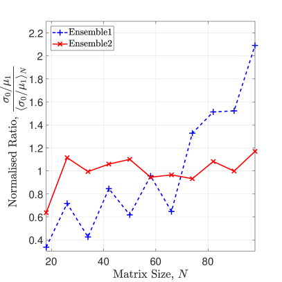
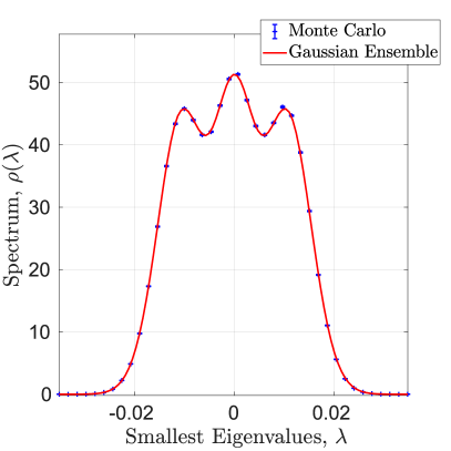
Figure 1: (a) Identification of former topological modes: A comparison of the ratio between the width of the smallest eigenvalue and the position of the second smallest eigenvalue as a function of the matrix size $N$ for Ensemble 1 ($\nu=1$) and Ensemble 2 ($\nu=0$) in Section V.2. We have normalised the mean of each curve. The coupling constant is set to $\alpha=0.01\sqrt{{\rm Tr}A^{-2}}||S||_{\rm op}/\sqrt{N}$ according to (III.15). The ensemble size is $10^{5}$. (b) The density of the smallest eigenvalues for Ensemble 4 with $n=33$ and $\nu=3$ from Section V.2. The Monte Carlo simulation (blue error bars, $10^{6}$ matrices generated) and the theoretical distribution of the GUE of size $3\times 3$ (red solid curve) are compared, see (V.52).

V.1 Application to Experiments

We wish to relate the scaling with $N$ to physical quantities. We here use a result from the $\epsilon$-regime of effective field theory, namely that the size of the matrix scales linearly with the volume of the system. We refer to RMT_2_EFT-1 ; RMT_2_EFT-2 for the full derivation, but the general idea is to calculate the non-linear $\sigma$-model (or chiral Lagrangian) of the random matrix model, which for all classes has the form

$$S = \int d^{4}x\left[{\rm Tr}\left(\partial_{\mu}U\partial^{\mu}U^{-1}\right)+{\rm Tr}M(U+U^{-1})\right].$$ (V.47)

The exact nature of the Goldstone field $U$ will depend on the class. As we consider the low-energy modes around the origin, where dynamics are frozen out DOTV ; GasserLeutwylerThermo ; GasserLeutwylerSym , the potential term becomes the most important. Constructing the Lagrangian directly from the matrix model leads to the identification $V\sim N$. This means that under the above assumptions, the width of the broadened modes scale as $\sqrt{V}$.

The proposed identifier is therefore the ratio $\sigma_{0}/\mu_{1}$, where $\sigma_{0}$ is the width of the ground state distribution, and $\mu_{1}$ is the mean position of the first excited state. If this scales significantly different from 1, it is safe to conclude a system with a broadened zero mode. This scaling is also found in the literature of lattice QCD and has helped to explain the unusual behaviour observed in lattice simulations DSV ; ADSV .

V.2 Example Ensembles

For the numerical checks, we compare the following four ensembles. We first draw a fixed $A^{(N)}$ and $S^{(N)}$ and then we average over $U$ for the Hamiltonian $K^{(N)}=A^{(N)}+\alpha US^{(N)}U^{\dagger}$.

Ensemble 1: To illustrate a particular condensed matter application we consider a direct sum of two antisymmetric matrices that are the same up to a sign, corresponding to particle-hole-symmetry Chiu ; BeenakkerRMT ; Neven . This ensemble is perturbed by off-diagonal blocks in order to model topological superconductors carrying Majorana modes. The ensemble has the form

$$K^{(N)} = \left(\begin{matrix}iM&0\\ 0&-iM\end{matrix}\right)+\alpha O\left(\begin{matrix}0&iW\\ -iW^{T}&0\end{matrix}\right)O^{T}\ ,\ M=-M^{T}\ .$$ (V.48)

The matrices $M$ and $W$ are real and of dimension $2n+\nu$, and $M$ is antisymmetric. So for $\alpha=0$ and $\nu=1$ the model exhibits two generic zero modes. The matrices are generated once via i.i.d. entries uniform on the interval $[-1,1]$ and then kept fixed. The ensemble average is only done via the orthogonal matrix $O$. The full matrix $K^{(N)}$ is of size $N=4n+2\nu$ and imaginary antisymmetric, and for $\alpha>0$ no exact modes are present. For $\nu=1$ the two zero modes are broadened by the coupling. They form a $2\times 2$ imaginary antisymmetric Gaussian ensemble.

Ensemble 2: To illustrate the different scalings of broadened zero eigenvalues and bulk eigenvalues, we also consider an ensemble for comparison of the form

$$K^{(N)}=iA^{(N)}+i\alpha OS^{(N)}O^{T}\ ,\ K^{(N)}={K^{(N)}}^{\dagger}=-{K^{(N)}}^{T}$$ (V.49)

with matrix size $N=2n$ and no further substructure. This ensemble never has exact zero modes in contrast to the models covered by our discussion. We again draw all matrix entries of $A$ and $S$ i.i.d. once, uniformly from the interval $[-1,1]$. Afterwards we keep them fixed and average over the orthogonal matrices $O$ only.

(a)                                                               (b)

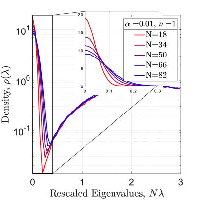
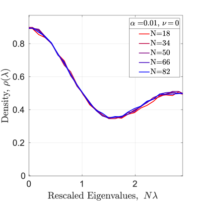
Figure 2: The microscopic density for Monte Carlo simulations of an ensemble with a single topological mode and one without (see V.48 and V.49) for different matrix sizes. Here we have also averaged over the spectrum for visual clarity. The eigenvalues have been rescaled according to (V.46) to keep the distance between the smallest eigenvalues of the order $1$. We compare the difference between a topological and a non-topological mode. We see the former topological mode broaden with $N$. The ensemble size is $10^{5}$ and the bin size is roughly $0.2$ for (a) plot and $0.1$ for (b). The density in (a) is shown on logarithmic scale to keep both peaks visible in the same plot, but a zoom-in is provided.

In Figure 2 we compare the microscopic densities about the origin for both Ensembles 1 and 2. In both plots we have rescaled the eigenvalues according to (V.46) to keep the mean inter-eigenvalue distance of order 1. We have also averaged over the spectrum of $A$ and $S$, which was not the case in Figure 1 (a). This is done to increase the contrast of the scaling of the eigenvalues with the volume $V$ represented by $N$. As predicted in Section V.1, the perturbed zero mode in Ensemble 1 changes with the volume in the rescaled variables, whereas the same does not happen for the smallest eigenvalue in Ensemble 2.

However, averaging over the spectrum is not necessary as we show in Figure 1 (a), where we plot the ratio $\sigma_{0}/\mu_{1}$ as a function of the matrix size $N$. We suggest this quantity as an identifier for topological or other system specific zero modes. We rescale $\alpha||S||_{\rm op}\sqrt{{\rm Tr}A^{-2}}/\sqrt{N}\to\alpha$ to keep the coupling constant on the same scale for all matrix sizes, see (III.15). As we do not average over the spectrum, the variance of the individual modes partially obscures the scaling, but it is still visible. If an average over the spectrum is also performed, the difference becomes even clearer, cf. Figure 2.

Ensemble 3: To illustrate that degeneracy of the perturbation is irrelevant as long as it satisfies the conditions (III.13-III.15), we consider an ensemble very similar to Ensemble 1, except that the perturbation is proportional to the second Pauli matrix. That is,

$$K^{(N)} = \left(\begin{matrix}iM_{1}&0\\ 0&iM_{2}\end{matrix}\right)+i\alpha O\left(\begin{matrix}0&\leavevmode\hbox{\small 1\kern-3.8pt\normalsize 1}\\ -\leavevmode\hbox{\small 1\kern-3.8pt\normalsize 1}&0\end{matrix}\right)O^{T}\ ,$$

$$M_{1}=-{M_{1}}^{T}\ ,\ M_{2}=-{M_{2}}^{T}\ .$$

$M_{1}$ and $M_{2}$ are real antisymmetric, but independent as the eigenvalues would otherwise be shifted rather than perturbed. These are chosen fixed with i.i.d. entries on the interval $[-1,1]$ while the average is over the orthogonal matrix $O$. With this ensemble we would like to emphasise the generality of the conditions (III.13-III.15). That is, the matrix Central Limit Theorem stated above describes the limit for a broad class of ensembles. This similarity is illustrated in Figure 3 where we compare Monte Carlo simulations to the corresponding theoretical curves derived in Section IV.

(a)                                                               (b)

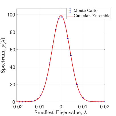
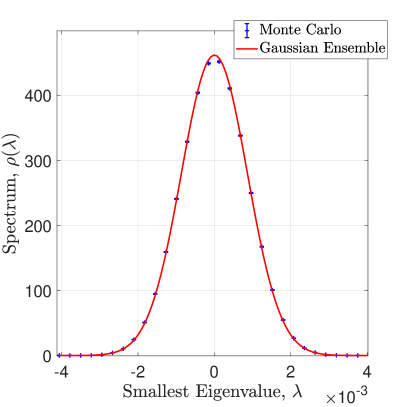
Figure 3: Distribution of the two smallest eigenvalues of Ensemble 1 (a) and Ensemble 3 (b) in Section V.2. In both ensembles the unperturbed Hamiltonian $A$ is imaginary, antisymmetric and block-diagonal of dimension $N=134$ so that it has two zero eigenvalues. The perturbation $S$ is a full generic imaginary matrix $i\alpha W$ (Ensemble 1) on the off-diagonal block and a constant matrix $i\alpha\leavevmode\hbox{\small 1\kern-3.8pt\normalsize 1}$ (Ensemble 3) with $\alpha=0.01$. The Monte Carlo simulations (blue error bars, $10^{6}$ matrices generated) are compared with our theoretical RMT predictions that are Gaussian distributions with the correct variances derived in Section IV (red solid curves).

Ensemble 4: As an application to QCD, more precisely lattice QCD, where chirality is broken by a perturbation DWW2011 ; DHS2012 ; KieburgWilson ; DSV ; ADSV ; MarioJacWilson , we consider the following model

$$K^{(N)} = \left(\begin{matrix}0&M\\ M^{\dagger}&0\end{matrix}\right)+\alpha USU^{\dagger}\ .$$ (V.51)

$M$ is a complex $(n+\nu)\times n$ matrix with no further symmetries, $S$ is a complex hermitian matrix, and $U$ is unitary and Haar-distributed. As before the only average we perform is over $U$. The index $\nu$ determines the number of exact zero modes, which allows us to have any number of broadened modes, unlike the antisymmetric ensembles. The $\nu$ zero modes from the chiral ensemble are all broadened by the perturbation, which is hermitian and has no further symmetry. This means that the former zero modes are distributed according to a Gaussian unitary ensemble of size $\nu\times\nu$ Mehta

$$\rho^{\nu}_{\rm GUE}(\lambda) = \frac{1}{2\sigma}\sum_{j=0}^{\nu-1}\varphi_{j}\left(\frac{\lambda}{\sigma}\right)^{2}\ ,$$ (V.52)

$$\varphi_{j}(\lambda) = \frac{1}{\sqrt{2^{j}j!\sqrt{\pi}}}e^{-\lambda^{2}/2}H_{j}(\lambda)$$

with $\sigma=\alpha\sqrt{{\rm Tr}(S^{(N)})^{2}/(\gamma N^{2})}$ the Hermite polynomials corresponding to the weight $e^{-\lambda^{2}}$. In Figure 1 (b) we compare the broadening of this ensemble to the theoretical prediction with the width found in Section IV.1.

VI Conclusion

We have presented a general mechanism explaining the observation of the universal broadening of degenerate eigenvalues inside a spectral gap when a generic perturbation is switched on. This universality states that the broadening follows the statistics of a finite-dimensional Gaussian random matrix ensemble. Exactly the finite dimensionality is surprising because one usually expects that spectral universality only holds in the limit of large matrix dimensions. This new universality relies on a self-average of the change of basis $U_{2}=\{\langle\psi_{j}|\phi_{l}\rangle\}_{j,l=N-\nu+1,\dots,N}$ between the unperturbed operator $A$ and the perturbation $S$ associated with the zero modes of $A$. In the present work, we have averaged over all bases transformations $U_{2}$ drawn from the Haar measure of the group associated to the respective symmetry class. Yet lattice simulations in QCD DelDebbio:2005qa ; DWW2011 ; DHS2012 ; CGRSZ strongly suggest that the measure can be relaxed to something non-uniform. As a further study it is natural to investigate what happens if the assumption of an average over the full Haar measure is loosened.

In our analysis, we quantified the conditions under which this universal broadening holds. The three conditions (III.13-III.15) are rather mild and have very natural physical interpretations like the relation between closing of the spectral gap and the coupling strength $\alpha$. Especially, we recover the critical scaling of $\alpha$ found in lattice QCD with Wilson fermions DelDebbio:2005qa ; DWW2011 ; DHS2012 ; CGRSZ and in the RMT-models for Majorana modes in disordered quantum wires AKMV ; KimAdam .

As a possible application we have suggested that our results may be used to distinguish topological modes in the bulk from modes in the bulk. The scaling behaviour in the system size and the coupling parameter $\alpha$ of the broadening for the eigenvalues of the two kind of modes is completely different. Consequently, this scaling might provide an ideal indicator of experiments.

Acknowledgements:

We would like to thank J. J. M. Verbaarschot and G. Akemann for interesting discussions on the subject. The first idea for the symmetry breaking in topological superconductors was conceived in collaboration with P. H. Damgaard, K. Flensberg, and E. B. Hansen. K. S. would like to thank A. Altland for discussions. Support by the German research council (DFG) through CRC 1283: “Taming uncertainty and profiting from randomness and low regularity in analysis, stochastics and their applications” (M. K.) and International Research Training Group 2235 Bielefeld-Seoul ”Searching for the regular in the irregular: Analysis of singular and random systems” (A. M.) is kindly acknowledged. A. M. would also like to thank Stony Brook University for their hospitality in October 2017 and ”Bielefeld Graduate School in Theoretical Sciences Mobility Grant” for funding the stay.

E-mail address:

M. Kieburg: mkieburg@physik.uni-bielefeld.de
A. Mielke: amielke@math.uni-bielefeld.de
K. Splittorff: split@nbi.ku.dk

References

• (1) M. L. Mehta, Random Matrices, (Third Edition, Academic Press, 2004).
• (2) T. Guhr, A. Müller-Groeling, and H. A. Weidenmüller, Random Matrix Theories in Quantum Physics: Common Concepts, Phys. Rept. 299, 189 (1998) [arXiv:cond-mat/9707301].
• (3) G. Akemann, J. Baik, and P. Di Francesco (eds.), The Oxford Handbook of Random Matrix Theory, (First Edition, Oxford University Press, 2015).
• (4) J. J. M. Verbaarschot and I. Zahed, Spectral density of the QCD Dirac operator near zero virtuality, Phys. Rev. Lett.  70, 3852 (1993) [arXiv:hep-th/9303012].
• (5) J. J. M. Verbaarschot, The Spectrum of the QCD Dirac operator and chiral random matrix theory: The Threefold way, Phys. Rev. Lett.  72, 2531 (1994) [arXiv:hep-th/9401059].
• (6) J. J. M. Verbaarschot, The Spectrum of the Dirac operator near zero virtuality for N(c) = 2 and chiral random matrix theory, Nucl. Phys. B 426, 559 (1994) [arXiv:hep-th/9401092].
• (7) P. H. Damgaard, J. C. Osborn, D. Toublan and J. J. M. Verbaarschot, The microscopic spectral density of the QCD Dirac operator, Nucl. Phys. B 547, 305 (1999) [arXiv:hep-th/9811212].
• (8) F. J. Dyson, The Threefold Way. Algebraic Structure of Symmetry Groups and Ensembles in Quantum Mechanics, J. Math. Phys. 3, 1199 (1962).
• (9) M. R. Zirnbauer, Riemannian Symmetric Superspaces and their Origin in Random Matrix Theory, J. Math. Phys. 37, 4986 (1996) [arXiv:math-ph/9808012].
• (10) M. Caselle, A New Classification Scheme for Random Matrix Theories, (1996) [arXiv:cond-mat/9610017 [cond-mat.stat-mech]].
• (11) D. Bernard and A. LeClair, A Classification of Non–Hermitian Random Matrices, Contribution to the Proceedings of the NATO Advanced Research Workshop on Statistical Field Theories, Como 18-23 June 2001 [arXiv:cond-mat/0110649 [cond-mat.dis-nn]].
• (12) U. Magnea, Random matrices beyond the Cartan classification, J. Phys. A: Math. Theor. 41, 045203 (2008) [arXiv:0707.0418 [math-ph]].
• (13) A. Hüffmann, Disordered Wires from a Geometric Viewpoint, J. Phys. A 23, 5733 (1990).
• (14) M. Caselle, A New Universality Class Describing the Insulating Regime of Disordered Wires with Strong Spin-Orbit Scattering, Mod. Phys. Lett. B 10, 681-688 (1996) [arXiv:cond-mat/9505068].
• (15) A. Altland and M. R. Zirnbauer, Random Matrix Theory of a Chaotic Andreev Quantum Dot, Phys. Rev. Lett. 76, 3420 (1996) [arXiv:cond-mat/9508026]; Novel Symmetry Classes in Mesoscopic Normal-Superconducting Hybrid Structures, Phys. Rev. B 55, 1142 (1997) [arXiv:cond-mat/9602137].
• (16) S. Ryu, A. P. Schnyder, A. Furusaki, and A. W. W. Ludwig, Topological insulators and superconductors: Tenfold way and dimensional hierarchy, New J. Phys. 12, 065010 (2010) [arXiv:0912.2157 [cond-mat.mes-hall]].
• (17) R. DeJonghe, K. Frey, and T. Imbo, Bott Periodicity and Realizations of Chiral Symmetry in Arbitrary Dimensions, Phys. Lett. B 718, 603 (2012) [arXiv:1207.6547 [hep-th]].
• (18) R. J. Slager, A. Mesaros, V. Juričić, C. L. Kane, and J. Zaanen, Topological classification of crystalline insulators through band structure combinatorics, Nature Physics 9, 98 (2013) [arXiv:1209.2610 [cond-mat.mes-hall]].
• (19) M. Kieburg, J. J. M. Verbaarschot, and S. Zafeiropoulos, A classification of 2-dim Lattice Theory, PoS LATTICE2013 337 (2014) [arXiv:1310.6948]; Dirac Spectra of 2-dimensional QCD-like theories, Phys. Rev. D 90, 085013 (2014) [arXiv:1405.0433 [hep-lat]].
• (20) C. K. Chiu, J. C. Y. Teo, A. P. Schnyder, and S. Ryu, Classification of topological quantum matter with symmetries, Rev. Mod. Phys. 88, no. 3, 035005 (2016) [arXiv:1505.03535 [cond-mat.mes-hall]].
• (21) J. Kruthoff, J. de Boer, J. van Wezel, C. L. Kane, and R. J. Slager, Topological classification of crystalline insulators through band structure combinatorics, Phys. Rev. X 7, no. 4, 041069 (2017) [arXiv:1612.02007 [cond-mat.mes-hall]].
• (22) M. Kieburg and T. R. Würfel, Shift of Symmetries of Naive Fermions in QCD-like Lattice Theories, Phys. Rev. D 96, 034502 (2017) [arXiv:1703.08083 [hep-lat]]; Global Symmetries of Naive and Staggered Fermions in Arbitrary Dimensions, EPJ Web Conf. 175, 04006 (2018) [arXiv:1710.03049].
• (23) A. Pandey and M. L. Mehta, Gaussian Ensembles Of Random Hermitian Matrices Intermediate Between Orthogonal and Unitary Ones, Commun. Math. Phys. 87, 449 (1983).
• (24) M.  L.  Mehta and A. Pandey, On Some Gaussian Ensembles of Hermitian Matrices, J. Phys. A: Math. Gen. 16, 2655 (1983).
• (25) P. J. Forrester, T. Nagao, and G. Honner, Correlations for the orthogonal-unitary and symplectic-unitary transitions at the hard and soft edges, Nucl. Phys. B 553, 601 (1999) [arXiv:cond-mat/9811142 [cond-mat.mes-hall]].
• (26) T. Nagao and P. J. Forrester, Quaternion determinant expressions for multilevel dynamical correlation functions of parametric random matrices, Nuclear Physics B 563, 547–572 (1999).
• (27) M. Katori, H. Tanemura, T. Nagao, and N. Komatsuda, Vicious walk with a wall, noncolliding meanders, and chiral and Bogoliubov-deGennes random matrices, Phys. Rev. E 68, 021112 (2003) [arXiv:cond-mat/0303573 [cond-mat.stat-mech]].
• (28) M. Katori and H. Tanemura, Infinite systems of non-colliding generalized meanders and Riemann-Liouville differintegrals, Probab. Th. Rel. Fields 138, 113 (2007) [arXiv:math/0506187 [math.PR]].
• (29) G. Akemann and T. Nagao, Random Matrix Theory for the Hermitian Wilson Dirac Operator and the chGUE-GUE Transition, JHEP 10, 060 (2011) [arXiv:1108.3035 [math-ph]].
• (30) T. Kanazawa and M. Kieburg, Symmetry Transition Preserving Chirality in QCD: A Versatile Random Matrix Model, Phys. Rev. Lett. 120, 242001 (2018) [arXiv:1803.04122 [hep-th]]; GUE-chGUE Transition preserving Chirality at finite Matrix Size, J. Phys. A: Math. Theor. 51, 345202 (2018) [arXiv:1804.03985 [math-ph]]; Symmetry Crossover Protecting Chirality in Dirac Spectra, (2018) [arXiv:1809.10602].
• (31) G. Akemann, M. Kieburg, A. Mielke, and P. Vidal, Preserving Topology while Breaking Chirality: From Chiral Orthogonal to Anti-symmetric Hermitian Ensemble [arXiv:1806.10977 [math-ph]].
• (32) P. Bougerol and J. Lacroix, Products of Random Matrices with Applications to Schrödinger Operators, (Birhäuser Basel, 1985).
• (33) R. Qiu and M. Wicks, Sums of Matrix-Valued Random Variables, Chapter 2 of Cognitive Networked Sensing and Big Data, (Springer, Berlin, 2013).
• (34) S. Kumar, Eigenvalue statistics for the sum of two complex Wishart matrices, EPL 107, 60002 (2014) [arXiv:1406.6638 [math-ph]].
• (35) G. Akemann and J. R. Ipsen, Recent exact and asymptotic results for products of independent random matrices, Acta Physica Polonica B 46, 1747–1784 (2015) [arXiv:1502.01667 [math-ph]].
• (36) G. Akemann, T. Checinski, and M. Kieburg, Spectral correlation functions of the sum of two independent complex Wishart matrices with unequal covariances, J. Phys. A: Math. Theor. 49, 315201 (2016) [arXiv:1509.03466 [math-ph]].
• (37) M. Kieburg, Additive Matrix Convolutions of Pólya Ensembles and Polynomial Ensembles, (2017) [arXiv:1710.09481 [math.PR]].
• (38) L. Del Debbio, L. Giusti, M. Luscher, R. Petronzio and N. Tantalo, Stability of Lattice QCD Simulations and the Thermodynamic Limit, JHEP 0602, 011 (2006) [arXiv:hep-lat/0512021].
• (39) A. Deuzeman, U. Wenger, and J. Wuilloud, Spectral properties of the Wilson Dirac operator in the $\varepsilon$-regime, JHEP 1112, 109 (2011) [arXiv:1110.4002 [hep-lat]]; Topology, Random Matrix Theory and the spectrum of the Wilson Dirac operator, PoS LATTICE2011, 241 (2011) [arXiv:1112.5160 [hep-lat]].
• (40) P. H. Damgaard, U. M. Heller, and K. Splittorff, Finite-Volume Scaling of the Wilson-Dirac Operator Spectrum, Phys. Rev. D 85, 014505 (2012) [arXiv:1110.2851]; New Ways to Determine Low-Energy Constants with Wilson Fermions, Phys. Rev. D 86, 094502 (2012) [arXiv:1206.4786 [hep-lat]]; Wilson chiral perturbation theory, Wilson-Dirac operator eigenvalues and clover improvement, PoS ConfinementX, 077 (2012) [arXiv:1301.3099 [hep-lat]].
• (41) M. Kieburg, J. J. M. Verbaarschot, and S. Zafeiropoulos, Spectral Properties of the Wilson Dirac Operator and random matrix theory, Phys. Rev. D 88, 094502 (2013) [ arXiv:1307.7251 [hep-lat]]; The Effect of the Low Energy Constants on the Spectral Properties of the Wilson Dirac Operator, PoS LATTICE2013, 117 (2014) [arXiv:1310.7009 [hep-lat]].
• (42) K. Cichy and S. Zafeiropoulos, Wilson chiral perturbation theory for dynamical twisted mass fermions vs lattice data—A case study, Comput. Phys. Commun.  237, 143 (2019) [arXiv:1612.01289 [hep-lat]]; K. Cichy, E. Garcia-Ramos, K. Splittorff, and S. Zafeiropoulos, The microscopic Twisted Mass Dirac spectrum and the spectral determination of the LECs of Wilson χ𝜒χ-PT, PoS LATTICE2015, 058 (2016) [arXiv:1510.09169 [hep-lat]].
• (43) H. Leutwyler and A. V. Smilga, Spectrum of Dirac operator and role of winding number in QCD, Phys. Rev. D 46, 5607 (1992).
• (44) E. V. Shuryak and J. J. M. Verbaarschot, Random matrix theory and Spectral Sum Rules for the Dirac Operator in QCD, Nucl. Phys. A 560, 306 (1993) [arXiv:hep-th/9212088].
• (45) A. M. Halasz and J. J. M. Verbaarschot, Effective Lagrangians and Chiral Random Matrix Theory, Phys. Rev. D 52, 2563 (1995) [arXiv:hep-th/9502096].
• (46) G. Akemann, P. H. Damgaard, U. Magnea and S. Nishigaki, Universality of random matrices in the microscopic limit and the Dirac operator spectrum, Nucl. Phys. B 487, 721 (1997) [arXiv:hep-th/9609174].
• (47) M. Srednicki, Quantum field theory, (Cambridge University Press, Cambridge, 2007).
• (48) D. A. Ivanov, The supersymmetric technique for random-matrix ensembles with zero eigenvalues, Journal of Mathematical Physics, Volume 43, Issue 1, 126-153 (2002) [arXiv:cond-mat/0103137].
• (49) A. Kitaev, Periodic table for topological insulators and superconductors, AIP Conf. Proc. 1134, 22 (2009) [arXiv:0901.2686 [cond-mat.mes-hall]].
• (50) M. Z. Hasan and C. L. Kane, Topological Insulators, Rev. Mod. Phys. 82, 3045 (2010) [arXiv:1002.3895 [cond-mat.mes-hall]].
• (51) D. Bagrets and A. Altland, Class $D$ Spectral Peak in Majorana Quantum Wires, Phys. Rev. Lett. 109, 227005 (2012) [arXiv:1206.0434 [cond-mat.mes-hall]].
• (52) C. W. J. Beenakker, Search for Majorana Fermions in Superconductors, Annu. Rev. Con. Mat. Phys. 4, 113 (2013) [arXiv:1407.2131 [cond-mat.mes-hall]].
• (53) F. Wilczek, Majorana and Condensed Matter Physics, [arXiv:1404.0637 [cond-mat.supr-con]].
• (54) C. W. J. Beenakker, Random-matrix theory of Majorana fermions and topological superconductors, Rev. Mod. Phys. 87, 1037 (2015) [arXiv:1407.2131 [cond-mat.mes-hall]].
• (55) S. R. Elliott and M. Franz, Colloquium: Majorana fermions in nuclear, particle, and solid-state physics Rev. Mod. Phys. 87, 137 (2015).
• (56) J. Alicea, Y. Oreg, G. Refael, F. von Oppen, and M. P. Fisher, Non-Abelian statistics and topological quantum information processing in 1D wire networks, Nature Physics volume 7, 412–417 (2011).
• (57) F. Zhang,C. L. Kane, and E. J. Mele, Time-Reversal-Invariant Topological Superconductivity and Majorana Kramers Pairs, Phys. Rev. Lett. 111, 056402 (2013) [arXiv:1212.4232 [cond-mat.supr-con]].
• (58) P. Neven, D. Bagrets, and A. Altland, Quasiclassical theory of disordered multi-channel Majorana quantum wires, New J. Phys. 15, 055019 (2013) [arXiv:1302.0747 [cond-mat.mes-hall]].
• (59) E. Dumitrescu, B. Roberts, S. Tewari, J. D. Sau, and S. Das Sarma, Majorana Fermions in Chiral Topological Ferromagnetic Nanowires, Phys. Rev. B 91, 094505 (2015) [arXiv:1410.5412 [cond-mat.supr-con]].
• (60) P. H. Damgaard, K. Splittorff and J. J. M. Verbaarschot, Microscopic Spectrum of the Wilson Dirac Operator, Phys. Rev. Lett.  105, 162002 (2010) [arXiv:1001.2937 [hep-th]].
• (61) G. Akemann, P. H. Damgaard, K. Splittorff and J. J. M. Verbaarschot, Spectrum of the Wilson Dirac Operator at Finite Lattice Spacings, Phys. Rev. D 83, 085014 (2011) [arXiv:1012.0752 [hep-lat]].
• (62) M. Kieburg, J. J. M. Verbaarschot, and S. Zafeiropoulos, Dirac Spectrum of the Wilson Dirac Operator for QCD with Two Colors, Phys. Rev. D 92, no. 4, 045026 (2015) [arXiv:1505.01784 [hep-lat]].
• (63) T. Guhr and B. Kälber, A new method to estimate the noise in financial correlation matrices, J. Phys. A: Math. Gen. 36, 3009 (2003) [arXiv:1609.04252 [hep-lat]]; M. Vyas, T. Guhr and T. H. Seligman, Multivariate analysis of short time series in terms of ensembles of correlation matrices, Sci. Rep. 8, no. 1, 14620 (2018) [arXiv:1801.07790 [physics.data-an]].
• (64) A. Mielke and K. Splittorff, Universal Distribution of Would-be Topological Zero Modes in Coupled Chiral Systems, Phys. Rev. D 95, 074516 (2017) [arXiv:1609.04252 [hep-lat]].
• (65) K. Wilson, Confinement of quarks, Phys. Rev. D 10, 2445 (1974) in New Phenomena in sub-nuclear physics, ed. A. Zichichi (Plenum, New York, 1977).
• (66) J. Gasser and H. Leutwyler, Thermodynamics of Chiral Symmetry, Phys. Lett. B 188, 477 (1987).
• (67) J. Gasser and H. Leutwyler, Spontaneously Broken Symmetries: Effective Lagrangians at Finite Volume, Nucl. Phys. B 307, 763 (1988).
• (68) M. Capitaine, C. Donati-Martin, Spectrum of deformed random matrices and free probability Advanced Topics in Random Matrices, Florent Benaych-Georges, Charles Bordenave, Mireille Capitaine, Catherine Donati-Martin, Antti Knowles (edited by F. Benaych-Georges, D. Chafaï, S. Péché, B. de Tilière) Panoramas et synthèses 53 (2018) [arXiv:1607.05560 [math.PR]].