Classifying Convex Bodies by their
Contact and Intersection Graphs

Abstract

Suppose that $A$ is a convex body in the plane and that $A_{1},\dots,A_{n}$ are translates of $A$. Such translates give rise to an intersection graph of $A$, $G=(V,E)$, with vertices $V=\{1,\dots,n\}$ and edges $E=\{uv\mid A_{u}\cap A_{v}\neq\emptyset\}$. The subgraph $G^{\prime}=(V,E^{\prime})$ satisfying that $E^{\prime}\subset E$ is the set of edges $uv$ for which the interiors of $A_{u}$ and $A_{v}$ are disjoint is a unit distance graph of $A$. If furthermore $G^{\prime}=G$, i.e., if the interiors of $A_{u}$ and $A_{v}$ are disjoint whenever $u\neq v$, then $G$ is a contact graph of $A$.

In this paper we study which pairs of convex bodies have the same contact, unit distance, or intersection graphs. We say that two convex bodies $A$ and $B$ are equivalent if there exists a linear transformation $B^{\prime}$ of $B$ such that for any slope, the longest line segments with that slope contained in $A$ and $B^{\prime}$, respectively, are equally long. For a broad class of convex bodies, including all strictly convex bodies and linear transformations of regular polygons, we show that the contact graphs of $A$ and $B$ are the same if and only if $A$ and $B$ are equivalent. We prove the same statement for unit distance and intersection graphs.

1 Introduction

Consider a convex body $A$, i.e., a convex, compact region of the plane with non-empty interior, and let $\mathcal{A}=\{A_{1},\ldots,A_{n}\}$ be a set of $n$ translates of $A$. Then $\mathcal{A}$ gives rise to an intersection graph $G=(V,E)$, where $V=\{1,\ldots,n\}$ and $E=\{uv\mid A_{u}\cap A_{v}\neq\emptyset\}$, and a unit distance graph $G^{\prime}=(V,E^{\prime})$, where $uv\in E^{\prime}$ if and only if $uv\in E$ and $A_{u}$ and $A_{v}$ have disjoint interiors. In the special case that $G=G^{\prime}$ (i.e., the convex bodies of $\mathcal{A}$ have pairwise disjoint interiors), we say that $G$ is a contact graph (also known as a touch graph or tangency graph). Thus, $A$ defines three classes of graphs, namely the intersection graphs $I(A)$, the unit distance graphs $U(A)$, and the contact graphs $C(A)$ of translates of $A$.

The study of intersection graphs has been an active research area in discrete and computational geometry for the past three decades. Numerous papers consider the problem of solving classical graph problems efficiently on various classes of geometric intersection graphs. From a practical point of view, the research is often motivated by the applicability of intersection graphs when modeling wireless communication networks and facility location problems. If a station is located at some point in the plane and is able to transmit to and receive from all other stations within some distance then the stations can be represented as disks in such a way that two stations can communicate if and only if their disks overlap.

Meanwhile, the study of contact graphs of translates of a convex body has older roots. It is closely related to the packings of such a body, which has a very long and rich history in mathematics going back (at least) to the seventeenth century, where research on the packings of circles of varying and constant radii was conducted and Kepler famously conjectured upon a 3-dimensional counterpart of such problems, the packing of spheres. An important notion in this area is that of the Hadwiger number of a body $K$, which is the maximum possible number of pairwise interior-disjoint translates $K_{i}$ of $K$ that each touch but do not overlap $K$. The Hadwiger number of $K$ is thus the maximum degree of a contact graph of translates of $K$. In the plane, the Hadwiger number is $8$ for parallelograms and $6$ for all other convex bodies. We refer the reader to the books and surveys by László and Gábor Fejes Tóth [8, 9] and Böröczky [1].

Another noteworthy result on contact graphs is the Circle Packing Theorem (also known as the Koebe–Andreev–Thurston Theorem): A graph is simple and planar if and only if it is the contact graph of some set of circular disks in the plane (the radii of which need not be equal). The result was proven by Koebe in 1935 [16] (see [10] for a streamlined, elementary proof). Schramm [21] generalized the circle packing theorem by showing that if a smooth planar convex body is assigned to each vertex in a planar graph, then the graph can be realized as a contact graph where each vertex is represented by a homothet (i.e., a scaled translation) of its assigned body.

In this paper we investigate the question of when two convex bodies $A$ and $B$ give rise to the same classes of graphs. We restrict ourselves to convex bodies $A$ that have the URTC property (unique regular triangle constructibility). This is the property that given two interior disjoint translates $A_{1},A_{2}$ of $A$ that touch, there are exactly two ways to place a third translate $A_{3}$ such that $A_{3}$ is interior disjoint from $A_{1}$ and $A_{2}$, but touches both. Convex bodies with the URTC property include all linear transformations of regular polygons except squares and all strictly convex bodies [11].

The main result of the paper is summarized in the following theorem.

Theorem 1.

Let $A$ and $B$ be convex bodies with the URTC property. Then each of the identities $I(A)=I(B)$, $U(A)=U(B)$, and $C(A)=C(B)$ holds if and only if the following condition is satisfied: there is a linear transformation $B^{\prime}$ of $B$ such that for any slope, the longest segments contained in $A$ and $B^{\prime}$, respectively, with that slope are equally long.

1.1 Other Related Work

Several papers have compared classes of intersection graphs of various geometric objects, see for instance [2, 4, 5, 12, 17]. Most of the results are inclusions between classes of intersection graphs of one-dimensional objects such as line segments and curves.

A survey by Swanepoel [22] summarizes results on minimum distance graphs and unit distance graphs in normed spaces, including bounds on the minimum/maximum degree, maximum number of edges, chromatic number, and independence number.

Perepelitsa [20] studied unit disk intersection graphs in normed planar spaces and showed that they are $\chi$-bounded in any such space. Kim et al. [13] improved Perepelitsa’s bound. For other work on intersection graphs of translates of a fixed convex body, see [6, 7, 14, 15].

In the area of computational geometry, Müller et al. [19] gave sharp upper and lower bounds on the size of an integer grid used to represent an intersection graph of translates of a convex polygon with corners at rational coordinates. Their results imply that for any convex polygon $R$ with rational corners, the problem of recognizing intersection graphs of translates of $R$ is in NP. On the contrary, it is open whether recognition of unit disk graphs in the Euclidean plane is in NP. Indeed, the problem is $\exists\mathbb{R}$-complete (and thus in PSPACE), and using integers to represent the center coordinates and radii of the disks in some graphs requires exponentially many bits [3, 18].

1.2 Preliminaries

We begin by defining some basic geometric concepts and terminology.

1.2.1 Convex Bodies and Graphs as Point Sets

For a subset $A\subset\mathbb{R}^{2}$ of the plane we denote by $A^{\circ}$ the interior of $A$. We say that $A$ is a convex body if $A$ is compact, convex, and has non-empty interior. We say that $A$ is symmetric if whenever $x\in A$, then $-x\in A$. It is well-known that if $A$ is a symmetric convex body, then the map $\left\|\cdot\right\|_{A}:\mathbb{R}^{2}\to\mathbb{R}_{\geq 0}$ defined by

$$\left\|x\right\|_{A}=\inf\{\lambda\geq 0\mid x\in\lambda A\},$$

is a norm. Moreover $A=\{x\in\mathbb{R}^{2}\mid\left\|x\right\|_{A}\leq 1\}$ and $A^{\circ}=\{x\in\mathbb{R}^{2}\mid\left\|x\right\|_{A}<1\}$.

It follows from these properties that for translates $A_{1}=A+v_{1}$ and $A_{2}=A+v_{2}$ it holds that $A_{1}\cap A_{2}\neq\emptyset$ if and only if $\left\|v_{1}-v_{2}\right\|_{A}\leq 2$ and $A_{1}^{\circ}\cap A_{2}^{\circ}\neq\emptyset$ if and only if $\left\|v_{1}-v_{2}\right\|_{A}<2$. This means that when studying contact, unit distance, and intersection graphs of a symmetric convex body $A$, we can shift viewpoint from translates of $A$ to point sets in $\mathbb{R}^{2}$ and their $\left\|\cdot\right\|_{A}$-distances: If $\mathcal{A}\subset\mathbb{R}^{2}$ is a set of points we define $I_{A}(\mathcal{A})$ and $U_{A}(\mathcal{A})$ to be the graphs with vertex set $\mathcal{A}$ and edge sets $\{(x,y)\in\mathcal{A}^{2}\mid x\neq y\text{ and }\|x-y\|_{A}\leq 2\}$ and $\{(x,y)\in\mathcal{A}^{2}\mid x\neq y\text{ and }\|x-y\|_{A}=2\}$, respectively. Moreover, if for all distinct points $x,y\in\mathcal{A}$ it holds that $\|x-y\|_{A}\geq 2$, we say that $\mathcal{A}$ is compatible with $A$ and define $C_{A}(\mathcal{A})$ to be the graph with vertex set $\mathcal{A}$ and edge set $\{(x,y)\in\mathcal{A}^{2}\mid x\neq y\text{ and }\|x-y\|_{A}=2\}$. Then $I_{A}(\mathcal{A}),U_{A}(\mathcal{A})$, and $C_{A}(\mathcal{A})$, respectively, are isomorphic to the intersection, unit distance, and contact graph of $A$ realized by the translates $(A+a)_{a\in\mathcal{A}}$. When studying contact, unit distance, and intersection graphs of a symmetric, convex body $A$ we will view them as being induced by point sets rather than by translates of $A$.

1.2.2 The URTC Property

We say that a (not necessarily symmetric) convex body $A$ in the plane has the URTC property if the following holds: For any two interior disjoint translates of $A$, call them $A_{1}$ and $A_{2}$, satisfying that $A_{1}\cap A_{2}\neq\emptyset$, there exists precisely two vectors $v\in\mathbb{R}^{2}$ such that for $i\in\{1,2\}$, $(A+v)^{\circ}\cap A_{i}^{\circ}=\emptyset$ but $(A+v)\cap A_{i}\neq\emptyset$. If $A$ is symmetric, this amounts to saying that for any two points $v_{1},v_{2}\in\mathbb{R}^{2}$ with $\left\|v_{1}-v_{2}\right\|_{A}=2$, the set $\{v\in\mathbb{R}^{2}\mid\left\|v-v_{1}\right\|_{A}=\left\|v-v_{2}\right\|_{A}=2\}$ has size two. Gehér [11] proved that a symmetric convex body $A$ has the URTC property if and only if the boundary $\partial A$ does not contain a line segment of length more than $1$ in the $\left\|\cdot\right\|_{A}$-norm.

1.2.3 Drawing of a Graph

A drawing of a graph $G\in I(A)$ as an intersection graph of a convex body $A$ is a point set $\mathcal{A}\subset\mathbb{R}^{2}$ and a set of straight line segments $\mathcal{L}$ such that $I_{A}(\mathcal{A})$ is isomorphic to $G$ and $\mathcal{L}$ is exactly the line segments between the points $u,v\in\mathcal{A}$ which are connected by an edge in $G$. We define a drawing of a graph $G$ as a contact and unit distance graph similarly.

1.2.4 Notation

For a norm $\left\|\cdot\right\|$ on $\mathbb{R}^{2}$ and a line segment $\ell$ with endpoints $a$ and $b$ we will often write $\left\|\ell\right\|=\left\|ab\right\|$ instead of $\left\|a-b\right\|$. Also, if $A$ is a symmetric convex body and $U,V\subset\mathbb{R}^{2}$, we define $d_{A}(U,V):=\inf\{\left\|uv\right\|_{A}\mid(u,v)\in U\times V\}$.

1.3 Structure of the Paper

In Section 2, we establish the sufficiency of the condition of Theorem 1, which is relatively straightforward.

In Section 3 we show how to reduce Theorem 1 to the case where the convex bodies are symmetric. For contact graphs, we then prove the following more general version of the necessity of the condition of Theorem 1 in Section 4.

Theorem 2.

Let $A$ and $B$ be symmetric convex bodies with the URTC property such that $A$ is not a linear transformation of $B$. There exists a graph $G\in C(A)$ such that for all $H\in C(B)$ and all subgraphs $H^{\prime}\subset H$, $G$ is not isomorphic to $H^{\prime}$. In particular $C(A)\setminus C(B)\neq\emptyset$.

As we will also discuss in Section 4 the same result holds if $C(X)$ is replaced by $U(X)$ for $X\in\{A,B\}$ everywhere in the theorem above. The proof is identical.

In Section 5 we prove the following result which combined with Theorem 2 yields the necessity of the condition of Theorem 1 for intersection graphs.

Theorem 3.

Let $A$ and $B$ be symmetric convex bodies. If there exists a graph $G\in C(A)$ such that for all $H\in C(B)$ and all subgraphs $H^{\prime}\subset H$, $G$ is not isomorphic to $H^{\prime}$, then $I(A)\neq I(B)$.

This result holds for general symmetric convex bodies. An improvement of Theorem 2 to general symmetric convex bodies (not necessarily having the URTC property) would thus yield a version of Theorem 1 that also holds for general convex bodies.

2 Sufficiency of the Condition of Theorem 1

This section establishes the sufficiency of the condition stated in Theorem 1 – this is the easy direction. It is worth noting that for this direction our result holds for general convex bodies.

Essentially, we show that the classes of contact, unit distance, and intersection graphs arising from a convex body $A$ are closed under linear transformations of $A$ and under operations on $A$ maintaining the signature of $A$ which we proceed to define.

Definition 4 (Profile).

Let $A\subset\mathbb{R}^{2}$ be a convex body. A profile through $A$ at angle $\theta\in[0,\pi)$ is a closed line segment $\ell_{\theta}$ of maximal length which has argument $\theta$ and is contained in $A$.

Definition 5 (Signature).

Let $A\subset\mathbb{R}^{2}$ be a convex body. The signature of $A$ is the function $\rho_{A}\colon[0,\pi)\to\mathbb{R}$ satisfying that for every $\theta\in[0,\pi)$, $\rho_{A}(\theta)=\left\lvert\ell_{\theta}\right\rvert$ is the length of a profile through $A$ at angle $\theta$.

Lemma 6.

Let $A\subset\mathbb{R}^{2}$ be a convex body and $v\in\mathbb{R}^{2}$ a vector with argument $\theta\in[0,2\pi)$ and magnitude $r$. Then

1. $(A+v)\cap A\neq\emptyset$ if and only if $r\leq\rho_{A}(\theta)$.

2. $(A+v)^{\circ}\cap A^{\circ}\neq\emptyset$ if and only if $r<\rho_{A}(\theta)$.

Proof.

First, suppose that $a\in(A+v)\cap A$. Then $a-v\in A$ and by convexity, the line segment $\ell$ from $a-v$ to $a$, which has length $r$ and argument $\theta$, is contained in $A$. It follows that $r\leq\rho_{A}(\theta)$. If further $a\in A^{\circ}$, there exists a vector $u$ of length $\epsilon>0$ and argument $\theta$ such that $a+u\in A$. It follows that $(A+v+u)\cap A\neq\emptyset$ implying that $r+\epsilon\leq\rho_{A}(\theta)$, so $r<\rho_{A}(\theta)$.

Second, suppose $r\leq\rho_{A}(\theta)$ and let $a,b$ be the endpoints of a profile, $\ell_{\rho}$, through $A$ at angle $\theta$ such that the vector from $a$ to $b$ has argument $\theta$. Then $a+v\in\ell_{\theta}$ as $r\leq\rho_{A}(\theta)=\left\lvert\ell_{\theta}\right\rvert$. It follows that $a+v\in A\cap(A+v)$ implying $A\cap(A+v)\neq\emptyset$. If further $r<\rho_{A}(\theta)$, then $a+v\neq b$. Let $c\in A$ be such that $a,b$ and $c$ are not colinear. (Such a point exists as $A$ has non-empty interior.) The interiors of the triangles with vertices $a,b,c$ and $a+v,b+v,c+v$ are contained in $A^{\circ}$ and $(A+v)^{\circ}$, respectively and their intersection is non-trivial. It follows that $A^{\circ}\cap(A+v)^{\circ}\neq\emptyset$, as desired.

∎

Second, the following lemma demonstrates closure of contact, unit distance, and intersection graphs under linear transformations.

Lemma 7.

Let $A\subset\mathbb{R}^{2}$ be a compact and connected subset of the plane and $M\colon\mathbb{R}^{2}\to\mathbb{R}^{2}$ be an invertible linear transformation. Then $C(A)=C(M(A))$, $U(A)=U(M(A))$, and $I(A)=I(M(A))$.

Proof.

Suppose that $A_{1},\dots,A_{n}$ is a realization of a graph $G$ as either a contact, unit distance, or intersection graph of $A$. Then $M(A_{1}),\dots,M(A_{n})$ is a realization of $G$ as a contact, unit distance, or intersection graph, respectively, of $M(A)$. ∎

Finally, we combine the above observations to prove our sufficient condition.

Theorem 8.

Let $A,B\subset\mathbb{R}^{2}$ be convex bodies. If there exists a linear transformation $M\colon\mathbb{R}^{2}\to\mathbb{R}^{2}$ such that the signatures of $A$ and of $M(B)$ are identical, i.e., $\rho_{A}=\rho_{M(B)}$, then $C(A)=C(B)$, $U(A)=U(B)$, and $I(A)=I(B)$.

Proof.

Having already established Lemma 7, it suffices to show that if $\rho_{A}=\rho_{B}$ then $C(A)=C(B)$, $U(A)=U(B)$, and $I(A)=I(B)$.

Let $A_{1},\dots,A_{n}\subset\mathbb{R}^{2}$ be translated copies of $A$ in the plane; let $v_{1},\dots,v_{n}\in\mathbb{R}^{2}$ be vectors satisfying $A_{i}=A+v_{i}$ for every $i\in[n]$; and let $n$ translated copies of $B$, $B_{1},\dots,B_{n}$, be defined by $B_{i}=B+v_{i}$ for $i\in[n]$. Now, consider any pair $(i,j)\in[n]^{2}$ and denote by $\theta_{i,j}$ and $r_{i,j}$ the argument and magnitude of the vector $v_{i}-v_{j}$. By Lemma 6, $A_{i}\cap A_{j}\neq\emptyset$ if and only if $r_{i,j}\leq\rho_{A}(\theta_{i,j})=\rho_{B}(\theta_{i,j})$, which is true if and only if $B_{i}\cap B_{j}\neq\emptyset$. Similarly, $A_{i}^{\circ}\cap A_{j}^{\circ}\neq\emptyset$ if and only if $B_{i}^{\circ}\cap B_{j}^{\circ}\neq\emptyset$. It follows that if $A_{1},\dots,A_{n}$ is a realization of a graph $G$ as a contact, unit distance, or intersection graph then $B_{1},\dots,B_{n}$ is a realization of $G$ as a contact, unit distance, or intersection graph, respectively.

∎

3 Reducing to Symmetric Convex Bodies

In this section we show that for proving the necessity of the condition of Theorem 1 it suffices to consider only symmetric convex bodies with the URTC property. We use the well-known trick in discrete geometry of considering the “symmetrization” of a convex body $A$, $K=\frac{1}{2}(A+(-A))$.

Lemma 9.

Let $A\subset\mathbb{R}^{2}$ be a convex body with signature $\rho_{A}$. Then $K=\frac{1}{2}(A+(-A))$ is a symmetric convex body with signature $\rho_{K}=\rho_{A}$.

Proof.

It is well-known and easy to check that $K$ is symmetric, bounded and convex. For the statement concerning the signature, let $\theta\in[0,\pi)$ be given. Consider a profile $\ell_{\theta}$ through $A$ at angle $\theta$. Then $\frac{1}{2}\left(\ell_{\theta}+(-\ell_{\theta})\right)\subset K$ is a line segment of the same length and argument as $\ell_{\theta}$ and hence, $\rho_{K}(\theta)\geq\rho_{A}(\theta)$. Conversely, consider a profile $\ell_{\theta}^{\prime}$ through $K$ at angle $\theta$ and let $\frac{1}{2}(a_{1}-a_{2})$ and $\frac{1}{2}(a_{3}-a_{4})$ be the endpoints of $\ell_{\theta}^{\prime}$ with $a_{1},\dots,a_{4}\in A$. Then the vector $v=\frac{1}{2}(a_{1}-a_{2})-\frac{1}{2}(a_{3}-a_{4})$ has argument $\theta$ and magnitude $\rho_{K}(\theta)$, but since

$$\frac{1}{2}(a_{1}-a_{2})-\frac{1}{2}(a_{3}-a_{4})=\frac{1}{2}(a_{1}+a_{4})-\frac{1}{2}(a_{2}+a_{3})$$

and $\frac{1}{2}(a_{1}+a_{4}),\frac{1}{2}(a_{2}+a_{3})\in A$ by convexity of $A$, there is a line segment from $\frac{1}{2}(a_{1}+a_{4})$ to $\frac{1}{2}(a_{2}+a_{3})$ in $A$ with the same argument and magnitude as $v$. It follows that $\rho_{K}(\theta)\leq\rho_{A}(\theta)$. ∎

Thus, for every convex body $A$ there is a symmetric convex body $K$ with the same signature and which by Theorem 8 therefore has the same contact, unit distance, and intersection graphs as $A$.

Proposition 10.

Let $A$ and $B$ be convex bodies such that $\rho_{A}=\rho_{B}$. Then $A$ has the URTC property if and only if $B$ has the URTC property. In particular this applies when $B=\frac{1}{2}(A+(-A))$ is the symmetrization of $A$.

Proof.

Suppose that $A$ has the URTC property. Let $B_{1}=B+v_{1}$ and $B_{2}=B+v_{2}$ be translates of $B$ satisfying that $B_{1}\cap B_{2}\neq\emptyset$ but $B_{1}^{\circ}\cap B_{2}^{\circ}=\emptyset$. Let $A_{1}=A+v_{1}$ and $A_{2}=A+v_{2}$. Since $\rho_{A}=\rho_{B}$,  Lemma 6 implies that $A_{1}\cap A_{2}\neq\emptyset$ but $A_{1}^{\circ}\cap A_{2}^{\circ}=\emptyset$. Again using Lemma 6 we obtain that for a vector $v_{3}$ it holds that $B+v_{3}$ intersects $B_{1}$ and $B_{2}$ but only at their boundary if and only if $A+v_{3}$ intersects $A_{1}$ and $A_{2}$ but only on at the boundary. As $A$ has the URTC property it follows that there are exactly two choices of $v_{3}$ such that $B+v_{3}$ intersect $B_{1}$ and $B_{2}$ but only at their boundary. Since $B_{1}$ and $B_{2}$ were arbitrary it follows that $B$ has the URTC property. The converse implication is identical. ∎

Combined with the work done in the main body of this paper (Section 4 and 5) Theorem 1 follows immediately:

Proof of Theorem 1.

We have already seen the sufficiency (Theorem 8) of the condition. Theorems 2 and 3 (to be proved in the following sections) give the necessity in case $A$ and $B$ are symmetric. Suppose now that $A$ and $B$ are arbitrary convex bodies with the URTC property satisfying that for any linear transformation $B^{\prime}$ of $B$, $\rho_{A}\neq\rho_{B^{\prime}}$. For $X\in\{A,B\}$ let $K_{X}=\frac{1}{2}(X+(-X))$. If there exists a linear transformation $T$ satisfying that $\rho_{K_{A}}=\rho_{T(K_{B})}$ then symmetri yields that $K_{A}=T(K_{B})=K_{T(B)}$. Applying Lemma 9 we obtain the contradiction that $\rho_{A}=\rho_{T(B)}$ and we conclude that for no linear transformation $T$ is $\rho_{K_{A}}=\rho_{T(K_{B})}$. Since $K_{A}$ and $K_{B}$ are symmetric and by Proposition 10 both have the URTC property, we conclude that $C(K_{A})\neq C(K_{B})$, $U(K_{A})\neq U(K_{B})$, and $I(K_{A})\neq I(K_{B})$. But $C(K_{X})=C(X)$, $U(K_{X})=U(X)$, and $I(K_{X})=I(X)$ for $X\in\{A,B\}$ by Theorem 8, so the result follows. ∎

4 Necessity for Contact and Unit Distance Graphs

In this section we prove the necessity of the condition of Theorem 1 in the case of contact graphs in the setting where $A$ and $B$ are symmetric. The proof for unit distance graphs is completely identical so we will merely provide a remark justifying this claim by the end of the section. The main result of the section is slightly more general than required since we will use it in the classification of intersection graphs.

4.1 Properties of the Signature

Towards proving the main theorem of the section, we prove three lemmas regarding the behaviour of the signature of a symmetric convex body. The content of the concluding lemma is as follows: If $A$ and $B$, are symmetric convex bodies satisfying that no linear map transforms $A$ into $B$, then there exists a finite set of angles, $\theta_{1},\dots,\theta_{n}$ and an $\varepsilon>0$, such that the signature of no linear transform of $B$ is $\varepsilon$-close to the signature of $A$ at every angle $\theta_{i}$. This observation motivates the constructions of the section to follow.

Lemma 11.

For a symmetric convex body $A\subset\mathbb{R}^{2}$ the signature $\rho_{A}\colon[0,\pi)\to\mathbb{R}$ is continuous.

Proof.

For $\theta\in[0,\pi)$ we define the rotation matrix $M_{\theta}=\begin{pmatrix}\cos\theta&-\sin\theta\\ \sin\theta&\cos\theta\end{pmatrix}$. We further let $e_{1}=(1,0)\in\mathbb{R}^{2}$. It is easy to check that the mapping $\theta\mapsto M_{\theta}e_{1}$ is a continuous map $[0,\pi)\to\mathbb{R}^{2}$. Furthermore, since any norm on $\mathbb{R}^{2}$ induces the same topology as that of the Euclidian norm, the map $\left\|\cdot\right\|_{A}:\mathbb{R}^{2}\to\mathbb{R}_{\geq 0}$ is continuous with respect to the standard topology on $\mathbb{R}^{2}$. Thus, the map $\varphi\colon[0,\pi)\to\mathbb{R}^{2}$ defined by $\varphi(\theta)=\frac{M_{\theta}e_{1}}{\|M_{\theta}e_{1}\|_{A}},$ is continuous. The conclusion follows as $\rho_{A}(\theta)=2\|\varphi(\theta)\|_{2}$. ∎

Lemma 12.

Let $A$ be a symmetric convex body. Let $K$ be the set of all non-singular linear maps $\mathbb{R}^{2}\to\mathbb{R}^{2}$ with topology induced by the operator norm. For each $\theta\in[0,\pi)$ the map $f_{\theta}\colon K\to\mathbb{R}_{\geq 0}$ defined by $f_{\theta}(T)=\rho_{T(A)}(\theta)$ is continuous.

Proof.

If $T$ is non-singular, $T(A)$ is also symmetric with non-empty interior and thus induces a norm $\left\|\cdot\right\|_{T(A)}$ on $\mathbb{R}^{2}$. Let $M_{\theta}$ be as in the proof of Lemma 11 and $v_{\theta}=M_{\theta}e_{1}$. Then

$$\rho_{T(A)}(\theta)=\frac{2\|v_{\theta}\|_{2}}{\|v_{\theta}\|_{T(A)}}.$$

Note that

$$\|v_{\theta}\|_{T(A)}=\inf\{\lambda\geq 0\mid v_{\theta}\in\lambda T(A)\}=\inf\{\lambda\geq 0\mid T^{-1}v_{\theta}\in\lambda A\}=\|T^{-1}v_{\theta}\|_{A},$$

and so it suffices to show that the mapping $T\mapsto T^{-1}v_{\theta}$ is a continuous map $K\to\mathbb{R}^{2}$. Now, for $T_{1},T_{2}\in K$,

$$\|T_{1}^{-1}v_{\theta}-T_{2}^{-1}v_{\theta}\|_{2}\leq\|T_{1}^{-1}-T_{2}^{-1}\|_{op}\|v_{\theta}\|_{2},$$

where $\|\cdot\|_{op}$ is the operator norm, so it suffices to show that the inversion $T\mapsto T^{-1}$ is a continuous map $K\to K$. It is a standard result from the literature that on the set of invertible elements of a unital Banach algebra, $\mathcal{A}$, the operation of inversion, $x\mapsto x^{-1}$, is continuous. Since $K$ is exactly the invertible elements of the Banach algebra of linear maps $\mathbb{R}^{2}\to\mathbb{R}^{2}$, the conclusion follows. ∎

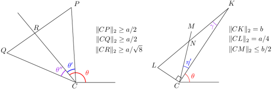
Figure 1: The two steps of the proof of Lemma 13

Lemma 13.

Let $A$ be a symmetric convex body and $a,b\in\mathbb{R}_{>0}$ constants. Consider some $\eta>0$ and suppose that for every $\theta\in[0,\pi)$ there exists $\theta^{\prime}\in[\theta,\theta+\eta)$ (with coordinates modulo $\pi$) such that $a\leq\rho(\theta^{\prime})\leq b$. If $\eta$ is sufficiently small as a function of $a$ and $b$, $\rho_{A}(\theta)<2b$ for every $\theta\in[0,\pi)$.

Proof.

We compute all coordinates modulo $\pi$. Also let $C$ be the center of $A$.

For the first part of the argument, see the left-hand side of Figure 1. We start by letting $\eta<\pi/4$. Then for arbitrary $\theta\in[0,\pi)$ there exists $\theta^{\prime},\theta^{\prime\prime}\in[0,\pi/4)$ and points $P,Q\in A$ such that the line segments $CP$ and $CQ$ have arguments $\theta-\theta^{\prime}$ and $\theta+\theta^{\prime\prime}$, respectively, and satisfy $\left\|CP\right\|_{2},\left\|CQ\right\|_{2}\geq\frac{a}{2}$. By convexity, the line segment $PQ$ is contained in $A$ and furthermore, it is easy to verify that every point on $PQ$ has distance at least $\frac{a}{\sqrt{8}}$ to $C$. Since the profile of $A$ at angle $\theta$ which passes through $C$ intersects $PQ$, it follows that $\rho_{A}(\theta)\geq\frac{a}{\sqrt{2}}$. Thus, for all $\theta\in[0,\pi)$, $\rho_{A}(\theta)\geq\frac{a}{\sqrt{2}}$.

For the remaining argument, see the right-hand side of Figure 1. Towards our main conclusion, suppose for contradiction that there is a line segment $CK$ of length $b$ and argument $\theta$ contained in $A$. Let $CL$ be the line segment of argument $\theta+\pi/2$ and length $a/4$ and note that it is contained in $A$. By assumption there exists a boundary point $M$ of $A$ such that $\left\|CM\right\|_{2}\leq b/2$ and $CM$ has argument $\theta+\eta^{\prime}$ where $0<\eta^{\prime}<\eta$. By convexity, $CM$ intersects $LK$ at a point $N$. Denote by $\gamma$ the angle $\angle CKL$ and note that it is a constant depending only on $a$ and $b$. Now, by the law of sines in $\triangle CKN$,

$$\left\|CN\right\|_{2}=\frac{b\sin(\gamma)}{\sin(\pi-\gamma-\eta^{\prime})}=b\cdot\frac{\sin(\gamma)}{\sin(\gamma+\eta^{\prime})},$$

so for $\eta$ sufficiently small as a function of $a$ and $b$, $\left\|CN\right\|_{2}>b/2$, which contradicts $\left\|CM\right\|_{2}\leq b/2$. ∎

Lemma 14.

Let $A$ and $B$ be symmetric convex bodies in $\mathbb{R}^{2}$. Suppose that for every finite set $\Theta\subset[0,\pi)$ and for every $\varepsilon>0$, there exists a linear map $T\colon\mathbb{R}^{2}\to\mathbb{R}^{2}$ satisfying that $|\rho_{T(B)}(\theta)-\rho_{A}(\theta)|<\varepsilon$ for all $\theta\in\Theta$. Then there exists a linear map $T\colon\mathbb{R}^{2}\to\mathbb{R}^{2}$ with $T(B)=A$.

Proof.

We may clearly assume that $A$ and $B$ are centered at the origin. For $n\in\mathbb{N}$, let $\Theta_{n}=\{i\pi/2^{n}\mid i\in[2^{n}]\}$; let $\varepsilon_{n}=1/n$; and let $T_{n}:\mathbb{R}^{2}\to\mathbb{R}^{2}$ be a linear map satisfying that $|\rho_{T_{n}(B)}(\theta)-\rho_{A}(\theta)|<\varepsilon_{n}$ for all $\theta\in\Theta_{n}$.

For $x\in\mathbb{R}^{2}$ and $r>0$ denote by $B_{r}(x)=\{y\in\mathbb{R}^{2}\mid\|x-y\|_{2}<r\}$ the open ball in the Euclidian norm with center $x$ and radius $r$. We begin by proving that $\{T_{n}\mid n\in\mathbb{N}\}$ is uniformly bounded in the operator norm by showing that there exists a constant $R>0$ such that $T_{n}(B)\subset B_{R}(0)$ when $n$ is sufficiently large. To this end, let $a=\inf_{\theta\in[0,\pi)}\rho_{A}(\theta)$ and $b=\sup_{\theta\in[0,\pi)}\rho_{A}(\theta)$ and note that $0<a,b<\infty$. There exists $N_{0}\in\mathbb{N}$ and constants $a^{\prime},b^{\prime}>0$ such that for every $n\geq N_{0}$, $a-\varepsilon_{n}\geq a^{\prime}$ and $b+\varepsilon_{n}\leq b^{\prime}$. This implies that for every $n\geq N_{0}$ and $\theta\in\Theta_{n}$, $a^{\prime}\leq\rho_{T_{n}(B)}(\theta)\leq b^{\prime}$. Applying Lemma 13, we find that there exists an $N_{1}\in\mathbb{N}$ such that for every $n\geq N_{1}$, $\rho_{T_{n}(B)}<2b^{\prime}$. Thus, $T_{n}(B)\subset B_{b^{\prime}}(0)$ for $n\geq N_{1}$ so $\{T_{n}\mid n\in\mathbb{N}\}$ is uniformly bounded. As it moreover holds for $n\geq N_{1}$ and $\theta\in\Theta_{n}(\theta)$ that $\rho_{T_{n}(B)}\geq a^{\prime}$, convexity of $T_{n}(B)$ gives that $\rho_{T_{n}(B)}\geq\frac{a^{\prime}}{\sqrt{2}}$ for $n\geq N_{1}$. In particular $T_{n}(B)\supset B_{a^{\prime}/\sqrt{8}}(0)$.

Since $(T_{n})_{n>0}$ is uniformly bounded we may by compactness assume that $(T_{n})_{n>0}$ converges in operator norm to some linear map $T:\mathbb{R}^{2}\to\mathbb{R}^{2}$ by passing to an appropriate subsequence. As moreover $T_{n}(B)\supset B_{a^{\prime}/\sqrt{8}}(0)$, it is easy to check that $T(B)\supset B_{a^{\prime}/\sqrt{8}}(0)$ so in particular $T$ is non-singular. We claim that $T(B)=A$. As $A$ and $T(B)$ are symmetric it suffices to show that $\rho_{A}=\rho_{T(B)}$. Moreover, $\rho_{A}$ and $\rho_{T(B)}$ are both continuous by Lemma 11 so since $\bigcup_{n\in\mathbb{N}}\Theta_{n}$ is dense in $[0,\pi)$ it suffices to show that $\rho_{A}|_{\Theta_{n}}=\rho_{T(B)}|_{\Theta_{n}}$ for each $n\in\mathbb{N}$. To see this let $\theta\in\bigcup_{n\in\mathbb{N}}\Theta_{n}$ and let $f_{\theta}$ be defined as in Lemma 12. Then $f_{\theta}$ is continuous so $f_{\theta}(T_{n})\to f_{\theta}(T)$ as $n\to\infty$ (here we use that $T$ is non-singular). It follows that

$$\rho_{T(B)}(\theta)=\lim_{n\to\infty}\rho_{T_{n}(B)}(\theta)=\rho_{A}(\theta),$$

as desired. This completes the proof. ∎

4.2 Establishing Necessity

Before proving the part of Theorem 1 concerning contact graphs we describe certain lattices which gives rise to contact graphs that can be realised in an essentially unique way. We start with the following definition.

Definition 15.

Let $A\subset\mathbb{R}^{2}$ be a symmetric convex body with the URTC property, and $\left\|\cdot\right\|_{A}$ the associated norm. Let $e_{1},e_{2}\in\mathbb{R}^{2}$ be such that $\left\|e_{1}\right\|_{A}=\left\|e_{2}\right\|_{A}=\left\|e_{1}-e_{2}\right\|_{A}=2$. We define the lattice $\mathcal{L}_{A}(e_{1},e_{2})=\{a_{1}e_{1}+a_{2}e_{2}\mid(a_{1},a_{2})\in\mathbb{Z}^{2}\}$.

Note that if $e_{1}$ has been chosen with $\|e_{1}\|_{A}=2$, then using the URTC property there are precisely two vectors $v$ with $\|v\|_{A}=\|v-e_{1}\|_{A}=2$. If one is $v_{2}$ the second is $e_{1}-v_{2}$ so regardless how we choose $e_{2}$ we obtain the same lattice. Let us describe a few properties of the lattice $\mathcal{L}_{A}(e_{1},e_{2})$. Using the triangle inequality and the URTC property of $A$ it is easily verified that for distinct $x,y\in\mathcal{L}_{A}(e_{1},e_{2})$, $\|x-y\|_{A}\geq 2$ with equality holding exactly if $x-y\in\mathcal{S}_{A}:=\{e_{1},e_{2},-e_{1},-e_{2},e_{1}-e_{2},e_{2}-e_{1}\}$. Another useful fact is the following:

Lemma 16.

With $\mathcal{S}_{A}$ as above it holds that $\frac{1}{2}\mathop{\mathrm{conv}}(\mathcal{S}_{A})\subset A\subset\mathop{\mathrm{conv}}(\mathcal{S}_{A})$. Here $\mathop{\mathrm{conv}}(\mathcal{S}_{A})$ is the convex hull of $\mathcal{S}_{A}$. If in particular $B$ is another symmetric convex body for which $\left\|e_{1}\right\|_{B}=\left\|e_{2}\right\|_{B}=\left\|e_{1}-e_{2}\right\|_{B}=2$, then for all $x\in\mathbb{R}^{2}$ it holds that $\frac{1}{2}\left\|x\right\|_{A}\leq\left\|x\right\|_{B}\leq 2\left\|x\right\|_{A}$.

Proof.

As $\frac{1}{2}\mathcal{S}_{A}\subset A$ and $A$ is convex the first inclusion is clear. For the second inclusion we note that all points $y$ on the hexagon connecting the points $e_{1},e_{2},e_{2}-e_{1},-e_{1},-e_{2},e_{1}-e_{2}$ of $\mathcal{S}_{A}$ in this order has $\|y\|_{A}\geq 1$ by the triangle inequality and so $A\subset\mathop{\mathrm{conv}}(\mathcal{S}_{A})$.

For the last statement of the lemma note that if $x\in\mathbb{R}^{2}$ then

$$\left\|x\right\|_{B} =\inf_{\lambda\geq 0}\{x\in\lambda B\}\geq\inf_{\lambda\geq 0}\{x\in\lambda\mathop{\mathrm{conv}}(\mathcal{S}_{B})\}$$

$$=\inf_{\lambda\geq 0}\{x\in\lambda\mathop{\mathrm{conv}}(\mathcal{S}_{A})\}\geq\inf_{\lambda\geq 0}\{x\in 2\lambda A\}=\frac{1}{2}\left\|x\right\|_{A},$$

and similarly $\|x\|_{A}\geq\frac{1}{2}\|x\|_{B}$. ∎

Definition 17.

We say that a graph $G=(V,E)$ is lattice unique if $|V|=n\geq 3$ and there exists an enumeration of its vertices $v_{1},\dots,v_{n}$ such that

• The vertex induced subgraph $G[v_{1},v_{2},v_{3}]\simeq K_{3}$ is a triangle.

• For $i>3$ there exists distinct $j,k,l<i$ such that $G[v_{j},v_{k},v_{l}]\simeq K_{3}$ and both $(v_{i},v_{j})$ and $(v_{i},v_{k})$ are edges of $G$.

Suppose that $A$ is a symmetric convex body with the URTC property, that $\mathcal{A}\subset\mathbb{R}^{2}$ is compatible with $A$, and that $G=C_{A}(\mathcal{A})$ is lattice unique. Enumerate the points of $\mathcal{A}=\{v_{1},\dots,v_{n}\}$ according to the definition of lattice uniqueness. Without loss of generality assume that $v_{1}=0$. Then the URTC property of $A$ combined with the lattice uniqueness of $G$ gives that $v_{4},\dots,v_{n}$ are uniquely determined from $v_{2}$ and $v_{3}$ and all contained in $\mathcal{L}_{A}(v_{2},v_{3})$. If moreover $B$ is another convex body with the URTC property, $\mathcal{B}=\{v_{1}^{\prime},\dots,v_{n}^{\prime}\}\subset\mathbb{R}^{2}$ has $v_{1}^{\prime}=0$ and is compatible with $B$, and $C_{B}(\mathcal{B})\simeq C_{A}(\mathcal{A})$ via the graph isomorphism $\varphi:v_{i}^{\prime}\mapsto v_{i}$, then the linear map $T:\mathbb{R}^{2}\to\mathbb{R}^{2}$ defined by $T:a_{1}v_{2}^{\prime}+a_{2}v_{3}^{\prime}\mapsto a_{1}v_{2}+a_{2}v_{3}$ satisfies that $T|_{\mathcal{B}}=\varphi$.

Before commencing the proof of Theorem 2 let us highlight the main ideas. The most important tool is Lemma 14 according to which there exist $\varepsilon>0$ and a finite set of directions $\Theta$ such that for any linear tranformation $B^{\prime}$ of $B$ there is a direction $\theta\in\Theta$ such that $\rho_{A}(\theta)$ and $\rho_{B^{\prime}}(\theta)$ differ by at least $\varepsilon$. We will construct $G$ by describing a finite set $\mathcal{A}\subset\mathbb{R}^{2}$ compatible with $A$, and defining $G=C_{A}(\mathcal{A})$. Now, $\mathcal{A}$ will be a disjoint union of two sets of points, $\mathcal{A}=\mathcal{U}\cup\mathcal{W}$, where $\mathcal{U}$ and $\mathcal{W}$ will play complementary roles. The construction will be such that $\mathcal{U}$ is a subset of a lattice $\mathcal{L}=\mathcal{L}_{A}(e_{1},e_{2})$ and such that the corresponding induced subgraph $G[\mathcal{U}]$ of $G$ is lattice unique. More precisely $\mathcal{U}$ will consist of $|\Theta|$ large hexagons connected along their edges. When attempting to realize $G$ as a contact graph of $B$ the lattice uniqueness enforces that $G[\mathcal{U}]$ is realized as a subgraph of a lattice $\mathcal{L}_{B}(e_{1}^{\prime},e_{2}^{\prime})$ in essentially the same way. The remaining points of $\mathcal{W}$ do not lie in the lattice $\mathcal{L}$. They constitute rigid beams in the directions from $\Theta$ “connecting” diagonally opposite points of the $|\Theta|$ hexagons of $\mathcal{U}$. The construction of $\mathcal{A}$ is depicted in the left-hand side of Figure 2 and in Figure 3. When trying to reconstruct the same contact graph (or a supergraph) with beams connecting the corresponding points of $\mathcal{U}^{\prime}$, we will find that in at least one direction the beam becomes too long or too short.

Proof of Theorem 2.

We let $e_{1},e_{2}\in\mathbb{R}^{2}$ be such that $\|e_{1}\|_{A}=\|e_{2}\|_{A}=\|e_{1}-e_{2}\|_{A}=2$ and define the lattice $\mathcal{L}:=\mathcal{L}_{A}(e_{1},e_{2})$. We also define the infinite graph $G_{0}:=C_{A}(\mathcal{L})$. Without loss of generality we can assume that $e_{1}$ and $e_{2}$ satisfy that $\|e_{1}\|_{2}=\|e_{2}\|_{2}=\|e_{1}-e_{2}\|_{2}=2$, since there exists a non-singular linear transformation $T$ such that $\|T(e_{1})\|_{2}=\|T(e_{2})\|_{2}=\|T(e_{1})-T(e_{2})\|_{2}=2$, and $C(A)=C(T(A))$. Note that in this setting we can use Lemma 16 to compare $A$ to the circle of radius 1 and obtain $\frac{1}{2}\|x\|_{2}\leq\|x\|_{A}\leq 2\|x\|_{2}$ for every $x\in\mathbb{R}^{2}$.

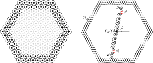
Figure 2: Left: The points of $\mathcal{H}_{6}$ along with the corresponding lattice unique subgraph $G_{0}[\mathcal{H}_{6}]$. Right: The attachment of the beam $\mathcal{B}_{\theta}(\ell)$.

As already mentioned we will construct $G$ by specifying a finite point set $\mathcal{A}\subset\mathbb{R}^{2}$ compatible with $A$ and define $G=C_{A}(\mathcal{A})$. The construction of $\mathcal{A}$ can be divided into several sub-constructions. We start out by describing a hexagon of points $\mathcal{H}_{k}$ for $k\in\mathbb{N}$ which satisfies that $C_{A}(\mathcal{H}_{k})$ is lattice unique.

Construction 18 ($\mathcal{H}_{k}$).

For an illustration of the construction see the left-hand side of Figure 2. For $x,y\in\mathcal{L}$ we write $d(x,y)$ for the distance between $x$ and $y$ in the graph $G_{0}$, and for $k\in\mathbb{N}$ we define $\mathcal{H}_{k}=\{x\in\mathcal{L}\mid d(x,0)\in\{k,k+1\}\}$. Clearly $G_{0}[\mathcal{H}_{k}]$ is a lattice unique graph. Moreover, using that $e_{1}$ and $e_{2}$ satisfy $\|e_{1}\|_{2}=\|e_{2}\|_{2}=\|e_{1}-e_{2}\|_{2}=2$ it is easy to check that the points $\{x\in\mathcal{L}\mid d(x,0)=k\}\subset\mathcal{H}_{k}$ lie on a regular hexagon $H_{k}$ whose corners have distance exactly $2k$ to the origin in the Euclidian norm. In particular the points $p\in\mathcal{H}_{k}$ has $\|p\|_{2}\geq\sqrt{3}k$, and thus $\|p\|_{A}\geq\frac{\sqrt{3}}{2}k$ by Lemma 16.

For a given $\theta\in[0,\pi)$ and $\ell\in\mathbb{N}$ we will construct a set of points $\mathcal{B}_{\theta}(\ell)\subset\mathbb{R}^{2}$ compatible with $A$ which constitute a “beam” of argument $\theta$:

Construction 19 ($\mathcal{B}_{\theta}{(\ell)}$).

Let $e_{\theta}\in\mathbb{R}^{2}$ be the vector of argument $\theta$ with $\|e_{\theta}\|_{A}=2$, and let $f_{\theta}\in\mathbb{R}^{2}$ be such that $\|f_{\theta}\|_{A}=\|f_{\theta}-e_{\theta}\|_{A}=2$ (by the URTC property we have two choices for $f_{\theta}$). For a given $\ell\in\mathbb{N}$ we define

$$\mathcal{B}_{\theta}(\ell)=\{ae_{\theta}\mid a\in\{-\ell,\dots,\ell\}\}\cup\{ae_{\theta}+f_{\theta}\mid a\in\{-\ell,\dots,\ell-1\}\}$$

Note that $\mathcal{B}_{\theta}(\ell)$ is compatible with $A$ and that $C(\mathcal{B}_{\theta}(\ell))$ is lattice unique.

For a given $k$ we want to choose $\ell$ as large as possible such that $\mathcal{B}_{\theta}(\ell)$ “fits inside” $G_{0}[\mathcal{H}_{k}]$. We then wish to “attach” $\mathcal{B}_{\theta}(\ell)$ to $G_{0}[\mathcal{H}_{k}]$ with extra points $\mathcal{S}$, the number of which does neither depend on $k$ nor on $\theta$. We wish to do it in such a way that $\mathcal{A}_{1}^{k}(\theta):=\mathcal{B}_{\theta}(\ell)\cup G_{0}[\mathcal{H}_{k}]\cup\mathcal{S}$ is compatible with $A$. The precise construction is as follows:

Figure 3: The final point set $\mathcal{A}$ where the point sets $\mathcal{C}_{k}(\theta)$ are “glued” together by translating them such that the contact graph realized by the union of the subsets $\mathcal{H}_{k}\subset\mathcal{C}_{k}(\theta)$ is lattice unique.

Construction 20 ($\mathcal{C}_{k}(\theta)$).

See Figure 2 (right). Consider the open line segment $L_{\theta}=\{re_{\theta}\mid r\in(-r_{\max},r_{\max})\}$ where $r_{\max}$ is maximal with the property that for all points $x\in L_{\theta}$ and all $y\in H_{k}$ it holds that $\|x-y\|_{A}>4$. Also let $\ell\in\mathbb{N}$ be maximal such that $\{ae_{\theta}\mid a\in\{-\ell,\dots,\ell\}\}\subset L_{\theta}$. Note that $\ell\geq\frac{\sqrt{3}}{4}k-3$ as the points $p\in H_{k}$ has $\|p\|_{A}\geq\frac{\sqrt{3}}{2}k$. If in particular $k>\frac{12}{\sqrt{3}-1}$ it holds that $\ell>\frac{k}{4}$.

When $\ell$ is chosen in this fashion, we have that $\mathcal{B}_{\theta}(\ell)$ is contained in the interior of $H_{k}$. Further, for all points $x\in\mathcal{B}_{\theta}(\ell)$ and all $y\in H_{k}$, it holds by the triangle inequality that $\|x-y\|_{A}>2$ since by construction every point of $\mathcal{B}_{\theta}(\ell)$ has distance at most 2 to $L_{\theta}$ in the norm $\left\|\cdot\right\|_{A}$. Now, $\mathcal{B}_{\theta}(\ell)$ will constitute our beam in direction $\theta$ and we will proceed to show that we can attach it to $\mathcal{H}_{k}$, as illustrated, using only a constant number of extra points. That this can be done is conceptually unsurprising but requires a somewhat technical proof.

For this we let $s>0$ be minimal with the property that there exists and $y\in\mathcal{H}_{k}$ such that $\|se_{\theta}-y\|_{A}=2$. As $d_{A}(L_{\theta},\mathcal{H}_{k})>4$ it holds that $s>\ell+1$. Define $\mathcal{S}_{1}(\theta)=\{se_{\theta},(s-1)e_{\theta},\dots,(s-s^{\prime})e_{\theta}\}$ where $s^{\prime}$ is chosen maximal such that $\mathcal{S}_{1}\cup\mathcal{B}_{\theta}(\ell)$ is compatible with $A$. In other words $s-s^{\prime}-1<1+\ell\leq s-s^{\prime}$. As $2\leq\|(s-s^{\prime})e_{\theta}-\ell e_{\theta}\|_{A}<4$ we can find at least one point $z_{1}^{\theta}\in\mathbb{R}^{2}$ such that $\|z_{1}^{\theta}-(s-s^{\prime})e_{\theta}\|_{A}=\|z_{1}^{\theta}-\ell e_{\theta}\|_{A}=2$ (this is one of the red copies of $A$ in Figure 2). It is easy to check that $\mathcal{B}_{\theta}(\ell)\cup\mathcal{S}_{1}(\theta)\cup\left\{z_{1}^{\theta}\right\}$ is compatible with $A$. To see that $\left\{z_{1}^{\theta}\right\}\cup\mathcal{H}_{k}$ is also compatible with $A$ we note that for any point $x\in\mathcal{H}_{k}$,

$$\|x-z_{1}^{\theta}\|_{A}\geq\|x-\ell e_{\theta}\|_{A}-\|\ell e_{\theta}-z_{1}^{\theta}\|_{A}\geq 4-2=2.$$

Finally, we need to argue that $\left\lvert\mathcal{S}_{1}(\theta)\right\rvert$ is bounded by a constant independent of $\theta$ and $k$. To this end let $P=\ell e_{\theta}$, $Q$ a point on $H_{k}$ of minimal Euclidian distance to $P$, and $R$ the intersection between $H_{k}$ and the line $\{re_{\theta}\mid r\in\mathbb{R}\}$. It is easy to check that the points $Q$ and $R$ lie on the same edge of $H_{k}$ and that the angle $\angle QPR\leq\pi/6$. It follows that $\left\|PR\right\|_{2}=\left\|PQ\right\|_{2}/\cos(\angle QPR)\leq\frac{2}{\sqrt{3}}\left\|PQ\right\|_{2}$. Combining this with the fact that $\left\|PQ\right\|_{2}\leq 2\left\|PQ\right\|_{A}\leq 2d_{A}(\{\ell e_{\theta}\},H_{k})\leq 12$ we obtain

$$\|se_{\theta}-\ell e_{\theta}\|_{A}\leq\left\|PR\right\|_{A}\leq 2\left\|PR\right\|_{2}\leq 16\sqrt{3}<28,$$

and so $\mathcal{S}_{1}(\theta)$ consists of at most $13$ points.

We may similarly define $\mathcal{S}_{2}(\theta)$ and $z_{2}^{\theta}$ to attach the other end of the beam, $\mathcal{B}_{\theta}(\ell)$. Letting $\mathcal{C}_{k}(\theta)=\mathcal{H}_{k}\cup\mathcal{B}_{\theta}(\ell)\cup\mathcal{S}_{1}(\theta)\cup\mathcal{S}_{2}\cup\left\{z_{1}^{\theta},z_{2}^{\theta}\right\}$ be the combination of the components completes the construction.

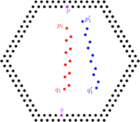
Figure 4: Situation from the argument that no graph in $C(B)$ has a subgraph isomorphic to $G$.

We are now ready to construct $\mathcal{A}$ which will consist of several translated copies $\mathcal{C}_{k}(\theta)$.

Construction 21 ($\mathcal{A}$).

By Lemma 14 we can find an $\varepsilon\in(0,1)$ and a finite set of directions $\Theta\subset[0,\pi)$ such that for all linear maps $T:\mathbb{R}^{2}\to\mathbb{R}^{2}$ there exists $\theta\in\Theta$ such that

$$\left|\frac{\rho_{A}(\theta)}{\rho_{T(B)}(\theta)}-1\right|\geq\varepsilon.$$

That we can scale the deviation to be multiplicative rather than additive is possible because $0<\inf_{\theta\in[0,\pi)}\rho_{A}(\theta)\leq\sup_{\theta\in[0,\pi)}\rho_{A}(\theta)<\infty$.

For each $\theta\in\Theta$ we construct a copy of $\mathcal{C}_{k}(\theta)=\mathcal{H}_{k}\cup\mathcal{B}_{\theta}(\ell)\cup\mathcal{S}_{1}(\theta)\cup\mathcal{S}_{2}(\theta)\cup\{z_{1}^{\theta},z_{2}^{\theta}\}$. We then choose translations $t_{\theta}\in\mathbb{R}^{2}$ for each $\theta\in\Theta$ such that $\bigcup_{\theta\in\Theta}(\mathcal{H}_{k}+t_{\theta})\subset\mathbb{R}^{2}$ is compatible with $A$ and induces a lattice unique contact graph. We can choose $(t_{\theta})_{\theta\in\Theta}$ in numerous ways to satisfy this. One is depicted in Figure 3. Another is obtained by enumerating $\Theta=\{\theta_{1},\dots,\theta_{q}\}$ and defining $t_{\theta_{i}}=((2k+3)e_{1}-(k+1)e_{2})\times(i-1)$. The exact choice is not important and picking one, we define $\mathcal{A}(k)=\bigcup_{\theta\in\Theta}(\mathcal{C}_{k}(\theta)+t_{\theta})$ which is a point set compatible with $A$. Lastly, we set $\mathcal{A}=\mathcal{A}\left(\left\lceil\frac{180}{\varepsilon}\right\rceil\right)$.

We are now ready for the final step of the proof:

Proving that no graph in $C(B)$ contains a subgraph isomorphic to $G=C_{A}(\mathcal{A})$.

Suppose for contradiction that there exists a set of points $\mathcal{B}\subset\mathbb{R}^{2}$ such that $G$ is isomorphic to a subgraph of $C_{B}(\mathcal{B})$. We may clearly assume that $|\mathcal{A}|=|\mathcal{B}|$ and we let $\varphi:\mathcal{A}\to\mathcal{B}$ be a bijection which is also a graph homomorphism when considered as a map $C_{A}(\mathcal{A})\to C_{B}(\mathcal{B})$. The points $\bigcup_{\theta\in\Theta}(\mathcal{H}_{k}+t_{\theta})$ induce a lattice unique contact graph of $A$. Thus, we may write $\bigcup_{\theta\in\Theta}(\mathcal{H}_{k}+t_{\theta})=\{p_{1},\dots,p_{n}\}$ such that $p_{1},p_{2}$ and $p_{3}$ induce a triangle of $G$ and such that for $i>3$ there exist distinct $j,k,l<i$ such that $p_{j},p_{k}$ and $p_{l}$ induce a triangle and such that $(p_{i},p_{k})$ and $(p_{i},p_{l})$ are edges of $G$. By translating the point sets $\mathcal{A}$ and $\mathcal{B}$ we may assume that $\varphi(p_{1})=p_{1}=0$. Then applying an appropriate linear transformation $T$, thus replacing $B$ by $T(B)$, we may assume that $\varphi(p_{2})=p_{2}$ and $\varphi(p_{3})=p_{3}$. Finally, the discussion succeeding Definition 17 implies that in fact $\varphi|_{\bigcup_{\theta\in\Theta}(\mathcal{H}_{k}+t_{\theta})}$ is the identity.

As noted in Construction 21, there exists $\theta\in\Theta$ such that $\left|\frac{\rho_{A}(\theta)}{\rho_{T(B)}(\theta)}-1\right|\geq\varepsilon$. The outline of the remaining argument is as follows: The Euclidian length of the beam $\mathcal{B}_{\theta}(\ell)$ is $2\ell\rho_{A}(\theta)$, but we will see that rigidity of $\bigcup_{\theta\in\Theta}(\mathcal{H}_{k}+t_{\theta})$ means that it is also $2\ell\rho_{T(B)}(\theta)+O(1)$. When $k$ (and hence $\ell$) is large enough, this will contradict the inequality above.

Formally, assume $t_{\theta}=0$ without loss of generality. Let $p,q\in\mathcal{H}_{k}$ be such that for some $x\in\mathcal{S}_{1}(\theta)$, $\|p-x\|_{A}=2$, and for some $y\in\mathcal{S}_{2}(\theta)$, $\|q-y\|_{A}=2$. Note that $\varphi(p)=p$ and $\varphi(q)=q$. Also define $p_{1}=\ell e_{\theta}$, $q_{1}=-\ell e_{\theta},p_{1}^{\prime}=\varphi(p_{1})$ and $q_{1}^{\prime}=\varphi(q_{1})$ (see Figure 4). Then

$$\left|\|p_{1}q_{1}\|_{T(B)}-\|p_{1}q_{1}\|_{A}\right|=\left|\|p_{1}q_{1}\|_{T(B)}-\|p_{1}^{\prime}q_{1}^{\prime}\|_{T(B)}\right|$$

$$\leq \left|\|p_{1}q_{1}\|_{T(B)}-\|p_{1}^{\prime}q_{1}\|_{T(B)}\right|+\left|\|p_{1}^{\prime}q_{1}\|_{T(B)}-\|p_{1}^{\prime}q_{1}^{\prime}\|_{T(B)}\right|\leq\|p_{1}p_{1}^{\prime}\|_{T(B)}+\|q_{1}q_{1}^{\prime}\|_{T(B)}.$$

Next, there is a path of length $\left\lvert\mathcal{S}_{1}(\theta)\right\rvert+2$ from $p$ to $p_{1}$ in $\mathcal{C}_{k}(\theta)$ with intermediate vertices $\left\{z_{1}(\theta)\right\}\cup\mathcal{S}_{1}(\theta)$. Combining this with Lemma 16 and the fact that $\varphi(p_{1})=p_{1}^{\prime}$, we find

$$\|p_{1}-p_{1}^{\prime}\|_{T(B)}\leq\|p_{1}-p\|_{T(B)}+\|p-p_{1}^{\prime}\|_{T(B)}\leq 2\|p_{1}-p\|_{A}+\|p_{1}-p\|_{A}\leq 6(|\mathcal{S}_{1}|+2)\leq 90.$$

Similarly, $\|q_{1}q_{1}^{\prime}\|_{T(B)}\leq 90$, so $\left|\|p_{1}q_{1}\|_{T(B)}-\|p_{1}q_{1}\|_{A}\right|\leq 180$. But on the other hand we have that $\ell>k/4$, and so arrive at the contradiction

$$\left|\|p_{1}q_{1}\|_{T(B)}-\|p_{1}q_{1}\|_{A}\right|=4\ell\left|\frac{\rho_{A}(\theta)}{\rho_{T(B)}(\theta)}-1\right|\geq 4\ell\varepsilon>k\varepsilon=\left\lceil\frac{180}{\varepsilon}\right\rceil\cdot\varepsilon\geq 180.\qed$$

Remark 22.

We claimed that the proof of the part of Theorem 1 concerning unit distance graphs is identical to the proof above. In fact, if we replace $C(X)$ by $U(X)$ for $X\in\{A,B\}$ in the statement of Theorem 2, the result remains valid. To prove it we would construct $\mathcal{A}$ in precisely the same manner. The important point is then that the comments immediately prior to Theorem 1 concerning the rigidity of the realization of lattice unique graphs remains valid. If in particular $\mathcal{B}\subset\mathbb{R}^{2}$ satisfies that $U_{A}(\mathcal{A})\simeq U_{A}(B)$ via the isomorphism $\varphi:\mathcal{A}\to\mathcal{B}$, we may assume that $\varphi|_{\bigcup_{\theta\in\Theta}(\mathcal{H}_{k}+t_{\theta})}$ is the identity as in the proof above. The remaining part of the argument comparing the lengths of the beams then carries through unchanged. In conclusion, we are only left with the task of proving Theorem 1 for intersection graphs.

5 Intersection Graphs

In this section we prove Theorem 3. Our proof strategy is as follows: Consider two convex bodies $A$ and $B$ as in the statement of the theorem. We construct an intersection graph $Q^{k}_{A}\in I(A)$ containing a cycle $\alpha_{k}$ such that in any drawing of $Q^{k}_{A}$ as an intersection graph, $\alpha_{k}$ is contained in a translation of the annulus $kA\setminus(k-1)A$. This allows us to view $\alpha_{k}$ as an upscaled copy of the boundary of $A$ with a precision error decreasing in $k$. Similarly, in any drawing of $Q^{k}_{A}$ as an intersection graph of $B$, the cycle $\alpha_{k}$ is an upscaled copy of the boundary of $B$. The idea is then to build contact graphs using $\alpha_{k}$ from distinct copies of $Q^{k}_{A}$. Since we know that $C(A)\neq C(B)$, it follows that $I(A)\neq I(B)$.

However, $\alpha_{k}$ is not a completely fixed figure since there are many drawings of $Q^{k}_{A}$ as an intersection graph. To capture this uncertainty, we introduce the concept of $\varepsilon$-overlap graphs.

Definition 23 ($\varepsilon$-overlap Graph).

Let $\varepsilon>0$ and $K\subset\mathbb{R}^{2}$ be a symmetric convex body, and let $v_{0},\ldots,v_{n-1}\subset\mathbb{R}^{2}$ be $n$ points in the plane. Suppose that for any $i,j\in[n]$, $\left\|v_{i}v_{j}\right\|_{K}\geq 2-\varepsilon$. A graph $G$ with vertex set $[n]$ and edge set satisfying

$$E(G)\subseteq\left\{(i,j)\in[n]^{2}\;\middle|\;\left\|v_{i}v_{j}\right\|_{K}\leq 2\right\}$$

is called an $\varepsilon$-overlap graph of $K$. We say that $\{v_{0},\ldots,v_{n-1}\}$ realize the graph $G$ as an $\varepsilon$-overlap graph of $K$. Further, we denote by $C_{\varepsilon}(K)$ the set of graphs that can be realized as $\varepsilon$-overlap graphs of $K$.

We will use $\alpha_{k}$ to build an $\varepsilon$-overlap graph where $\varepsilon=O\left(\frac{1}{k}\right)$. We place copies of $Q^{k}_{A}$ centered at every point $v_{0},\ldots,v_{n-1}\in\mathbb{R}^{2}$, which are the vertices of the graph, and say that there is an edge between two points $v$, $v^{\prime}$ if the corresponding cycles $\alpha_{k}$, $\alpha_{k}^{\prime}$ intersect. Then using the following reduction from $\varepsilon$-overlap graphs to contact graphs finishes our proof.

Lemma 24.

Consider a graph $G^{\prime}=(V,E^{\prime})$ with $V=[n]$ and a convex body $A$. If for every $\varepsilon>0$, $G^{\prime}\in C_{\varepsilon}(A)$, then there is a graph $G=(V,E)\in C(A)$ such that $E^{\prime}\subseteq E$.

Proof.

Let $\varepsilon_{m}$ be a positive sequence such that $\varepsilon_{m}\longrightarrow 0$ as $m\longrightarrow\infty$ and suppose that $\mathcal{A}^{m}=\{v^{m}_{1},\ldots,v^{m}_{n}\}\subset\mathbb{R}^{2}$ realize $G^{\prime}$ as an $\varepsilon_{m}$-overlap graph. We may clearly assume that the values $\|v^{m}_{i}\|_{A}$ are bounded. By passing from $\mathcal{A}^{m}$ to a subsequence, we may therefore assume that for each $i\in V$, $v^{m}_{i}$ converges to some point $v_{i}$ as $m\longrightarrow\infty$. Clearly, $\|v_{i}v_{j}\|_{A}\geq 2$, so $\{v_{1},\ldots,v_{n}\}$ are compatible with $A$ and define a contact graph $G=(V,E)=C_{A}(\{v_{1},\ldots,v_{n}\})$. Furthermore, if $ij\in E^{\prime}$, then $\|v_{i}v_{j}\|_{A}\leq 2$, so $E^{\prime}\subseteq E$. ∎

Combining this with Theorem 2 will exactly give us our result. So the rest of this section will be dedicated to showing that the graph $Q^{k}_{A}$ exists and describe how to build $\varepsilon$-overlap graphs using it.

In the construction of $Q^{k}_{A}$ we have a designated vertex $s_{0}$ with the property that for every drawing of $Q^{k}_{A}$ as an intersection graph and every vertex $v\in\alpha_{k}$, we have $\left\|s_{0}v\right\|_{A}=\Omega(k)$. To obtain this property, we first construct another graph $P^{k}_{A}$ (which will be contained in $Q^{k}_{A}$) with a vertex $s_{0}$ such that in every drawing of $P^{k}_{A}$ as an intersection graph, $s_{0}$ is contained in $k$ nested disjoint cycles. A priori, it is not clear what it means for $s_{0}$ to be contained in a cycle of the graph in every drawing, since the drawing is not necessarily a plane embedding of the graph. However, as the following lemma shows, it is well-defined if $P^{k}_{A}$ is triangle-free.

Lemma 25.

If $G$ is a triangle-free graph then every drawing of $G$ as an intersection graph is a plane embedding.

Proof.

The proof will be by contraposition so assume that $A\subset\mathbb{R}^{2}$ is a convex body and that $G=(V,E)$ is a drawing as an intersection graph. Then there exists $x,y,z,w\in V$ with $xy,zw\in E$ and where the edges $xy$ and $zw$ intersect. Call this intersection point $p\in\mathbb{R}^{2}$. We know that $\left\|xy\right\|_{A}\leq 2$ and $\left\|zw\right\|_{A}\leq 2$. Using the triangle inequality we get that

$$\left\|xw\right\|_{A} \leq\left\|xp\right\|_{A}+\left\|wp\right\|_{A}$$

$$\left\|yz\right\|_{A} \leq\left\|yp\right\|_{A}+\left\|zp\right\|_{A}$$

combining this we get that

$$\left\|xw\right\|_{A}+\left\|yz\right\|_{A}\leq\left\|xy\right\|_{A}+\left\|zw\right\|_{A}\leq 4$$

since $p$ lies on the lines $xy$ and $zw$. This implies that either $\left\|xw\right\|_{A}\leq 2$ or $\left\|yz\right\|_{A}\leq 2$ so either $xw\in E(G)$ or $yz\in E(G)$. An analogous argument shows that either $xz\in E(G)$ or $yw\in E(G)$. This shows that $G$ contains a triangle which finishes the proof. ∎

We are now ready to define $P^{k}_{A}\in I(A)$ for any $k>0$. Besides being triangle-free, our aim is that $P^{k}_{A}$ should have the following properties:

1. There is a vertex $s_{0}$ such that in any drawing of $P_{A}^{k}$ as an intersection graph of $A$ and $B$, $s_{0}$ is contained in $k$ nested disjoint, simple cycles $\sigma_{1},\ldots,\sigma_{k}$.

2. There is a path $\kappa_{k}$ from a vertex $s_{k}$ to a leaf $t_{k}$ such that in any drawing of $P_{A}^{k}$ as an intersection graph of $A$ and $B$, the path $\kappa_{k}$ is on the boundary of the outer face.

Construction 26 ($P_{A}^{k}$.).

As in the previous section choose $e_{1},e_{2}\in\mathbb{R}^{2}$ such that $\left\|e_{1}\right\|_{A}=\left\|e_{2}\right\|_{A}=\left\|e_{1}-e_{2}\right\|_{A}=2$, let $\mathcal{L}:=\mathcal{L}(e_{1},e_{2})$, and put $G_{0}=I_{A}(\mathcal{L})$. We will define $P_{A}^{k}$ to be of the form $G_{0}[\mathcal{A}_{k}]$ for some $\mathcal{A}_{k}\subset\mathcal{L}$ to be defined inductively. Let first $s_{0}=0$, $t_{0}=e_{1}$, and $\mathcal{A}_{0}=\{s_{0},t_{0}\}$. Define $\kappa_{0}$ to be the length-one path between $s_{0}$ and $t_{0}$ in $G_{0}$. Suppose inductively that $\mathcal{A}_{k-1}$ has been defined. Write $t_{k-1}=(r-1)e_{1}$ for some positive integer $r$ and define $\mathcal{R}_{r}=\{x\in\mathcal{L}\mid d_{G_{0}}(x,0)=r\}$ and $\mathcal{K}_{r}=\{x\in G_{0}\mid d_{G_{0}}(re_{1},x)=1\}$. Define $\tau_{k}$ and $\sigma_{k}$ to be the cycles of $G_{0}$ through the points of $\mathcal{K}_{r}$ and $(\mathcal{R}_{r}\setminus\{re_{1}\})\cup(\mathcal{K}_{r}\setminus\{t_{k-1}\})$, respectively. Finally define $\mathcal{T}_{r}=\{t_{r-1}+ie_{1}\mid i=3,\dots,\ell\}$ where $\ell$ is chosen so large that the path $\kappa_{k}$ on the vertices of $\mathcal{T}_{r}$ is so long that it cannot be contained in the cycle $\sigma_{k}$ in any drawing of $P^{k}_{A}$ as an intersection graph of $A$ and $B$. Let $t_{k}=\ell e_{1}$ and $\mathcal{A}_{k}=\mathcal{A}_{k-1}\cup(\mathcal{R}_{r}\setminus\{re_{1}\})\cup\mathcal{K}_{r}\cup\mathcal{T}_{r}$. See Figure 5.

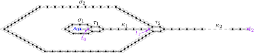
Figure 5: The construction of $P_{A}^{2}$.

Lemma 27.

The graph $P_{A}^{k}$ has properties 1–2.

Proof.

The graph $P_{A}^{0}$ trivially has the properties. Suppose inductively that the $P_{A}^{k-1}$ has the properties and consider any drawing of $P^{k}_{A}$ as an intersection graph of $A$ or $B$. Note that $\kappa_{k}$ is attached to two cycles: $\tau_{k}$ and $\sigma_{k}$. By construction, $\kappa_{k}$ is so long that it cannot be contained in any of them. Hence, $\kappa_{k}$ is in the exterior of both. It follows that either $\sigma_{k}$ is contained in $\tau_{k}$ or $\tau_{k}$ is contained in $\sigma_{k}$. Clearly, $\tau_{k}$ is too short for the first to be the case. We therefore get that all of $P_{A}^{k-1}$ is contained in $\sigma_{k}$ and that $\kappa_{k}$ is on the boundary of the outer face. Furthermore, the induction hypothesis implies that $s_{0}$ is contained in the $k$ nested, disjoint cycles $\sigma_{1},\ldots,\sigma_{k}$. ∎

The most important property of $P^{k}_{A}$ is that every vertex $u\in\sigma_{k}$ has distance $\Omega(k)$ to $s_{0}$ in any drawing of $P^{k}_{A}$ as intersection graph of $A$ and $B$. This is exactly what we will use when constructing $Q^{k}_{A}$.

Lemma 28.

Let $X\in\{A,B\}$. Consider any drawing of $P_{A}^{k}$ as an intersection graph of $X$. For any vertex $u\in\sigma_{k}$, we have $\left\|s_{0}u\right\|_{X}>2(k/9-1)$.

Proof.

Note that each cycle $\sigma_{1},\ldots,\sigma_{k}$ has an edge that intersects the segment $s_{0}u$, and that the intersection point has distance at most $1$ to a vertex of the cycle. We claim that each subsegment $r$ of $s_{0}u$ of length at most $2$ is intersected by at most $9$ cycles. Otherwise, the midpoint $x$ of $r$ would have distance at most $2$ to at least $10$ independent vertices. The translates of $X$ centered at these vertices are pairwise disjoint and contained in a ball $D$ centered at $x$ with radius $3$. But the area of $D$ is only $3^{2}=9$ times larger than that of $X$, a contradiction.

Let now $\ell=\left\|s_{0}u\right\|_{X}$, and divide $s_{0}u$ into $\lceil\ell/2\rceil$ equally long pieces, each of length at most $2$. As each piece is intersected by at most $9$ cycles, the total number of cycles intersecting $s_{0}u$ is $9\lceil\ell/2\rceil$. We get that $k\leq 9\lceil\ell/2\rceil<9(\ell/2+1)$ so that $\ell>2(k/9-1)$. ∎

Having defined $P^{k}_{A}$ we are now ready to the main part of this section: Constructing $Q^{k}_{A}$ and prove that it has the necessary properties for building $\varepsilon$-overlap graphs.

Construction 29 ($Q_{A}^{k}$).

We here define a graph $Q_{A}^{k}\in I(A)$ by specifying a drawing of $Q_{A}^{k}$ as an intersection graph of $A$. Let $k^{\prime}:=18(k+1)$. We start with $P_{A}^{k^{\prime}}$ and explain what to add to obtain $Q_{A}^{k}$. Let $u_{0},\ldots,u_{n-1}$ be the vertices of $\sigma_{k^{\prime}}$ in cyclic, counter-clockwise order. Consider an arbitrary drawing of $P_{A}^{k^{\prime}}$ as an intersection graph of $A$ and a vertex $u_{i}$. Note that $d:=\left\lceil\frac{\left\|s_{0}u_{i}\right\|_{A}-2}{2}\right\rceil$ is the number of vertices needed to add in order to create a path from $s_{0}$ to $u_{i}$. It follows from Lemma 28 that $d\geq 2k$.

We want to minimize the vector of these values $d$ with respect to each vertex $u_{i}\in\sigma_{k^{\prime}}$. To be precise, we define

$$(d_{0},\ldots,d_{n-1}):=\min\left(\left\lceil\frac{\left\|s_{0}u_{0}\right\|_{A}-2}{2}\right\rceil,\ldots,\left\lceil\frac{\left\|s_{0}u_{n-1}\right\|_{A}-2}{2}\right\rceil\right),$$

where the minimum is with respect to the lexicographical order and taken over all drawings of $P_{Q}^{k^{\prime}}$ as an intersection graph. Consider an drawing of $P_{A}^{k^{\prime}}$ as an intersection graph realizing the minimum and let $\mathcal{P}$ be the set of vertices in the drawing. For each vertex $u_{i}$, we create a path $\pi_{i}$ from $s_{0}$ to $u_{i}$ as follows. Let $\mathbf{v}_{i}$ be the unit-vector in direction $u_{i}-s_{0}$. We add new vertices placed at the points $v_{i}(j):=s_{0}+2j\mathbf{v}_{i}$ for $j\in\{1,\ldots,d_{i}\}$. We now define the vertices of $Q_{A}^{k}$ as $\mathcal{Q}:=\mathcal{P}\cup\bigcup_{i=0}^{n-1}\{v_{i}(1),\ldots,v_{i}(d_{i})\}$ and define $Q_{A}^{k}=I_{A}(\mathcal{Q})$. See Figure 6.

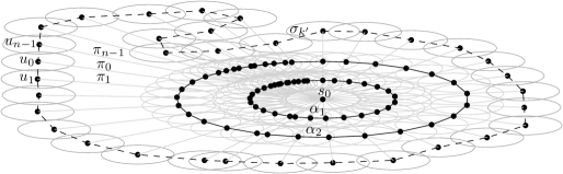
Figure 6: A part of a graph $Q_{A}^{k}$. The vertices $v_{i}(j)$ are only shown for $j\in\{1,2\}$, and only edges on paths $\pi_{i}$ and cycles $\alpha_{1},\alpha_{2},\sigma_{k^{\prime}}$ are shown.

Remark 30.

By construction, there exists a drawing of $Q_{A}^{k}$ as an intersection graph of $A$. If there does not exist one with respect to $B$, we are done, since we then clearly have that $I(A)\neq I(B)$. Now suppose that there exists a drawing of $P_{A}^{k^{\prime}}$ as an intersection graph of $B$ such that

$$\left(\left\lceil\frac{\left\|s_{0}u_{0}\right\|_{B}-2}{2}\right\rceil,\ldots,\left\lceil\frac{\left\|s_{0}u_{n-1}\right\|_{B}-2}{2}\right\rceil\right)\prec(d_{0},\ldots,d_{n-1}),$$ (1)

where $\prec$ denotes the lexicographical order. We can now define a graph $Q_{B}^{k}\in I(B)$ in a similar way as we defined $Q_{A}^{k}$ by adding $\left\lceil\frac{\left\|s_{0}u_{i}\right\|_{B}-2}{2}\right\rceil$ vertices to form a path from $s_{0}$ to each $u_{i}$. It then follows from (1) that $Q_{B}^{k}\notin I(A)$, so in this case we have likewise succeeded in proving $I(A)\neq I(B)$. In the following, we therefore assume that $Q_{A}^{k}\in I(B)$ for any $k$ and that no drawing of $P_{A}^{k^{\prime}}$ as an intersection graph of $B$ satisfying (1) exists.

First we need to show that $Q^{k}_{A}$ does contain a cycle $\alpha_{k}$ as described in the beginning of this section.

Lemma 31.

The set of edges of $Q_{A}^{k}$ contain the pairs $v_{i}(j)v_{i+1}(j)$ for any $i\in[n]$ and $j\in\{1,\ldots,k\}$, and for each $j\in\{1,\ldots,k\}$, these edges thus form a cycle $\alpha_{j}$. In the specific drawing of $Q^{k}_{A}$ as an intersection graph defined in Construction 29, the cycle $\alpha_{j}$ is contained in the annulus $\left\{x\in\mathbb{R}^{2}\;\middle|\;\left\|s_{0}x\right\|_{A}\in[2j-1,2j]\right\}$.

Proof.

Consider the pair $v_{i}(j)v_{i+1}(j)$. Note that $\left\|u_{i}u_{i+1}\right\|_{A}\leq 2$ as $u_{i}u_{i+1}$ is an edge of $\sigma_{k^{\prime}}$. Assume without loss of generality that $\left\|s_{0}u_{i}\right\|_{A}\leq\left\|s_{0}u_{i+1}\right\|_{A}$, and let $u^{\prime}_{i+1}$ be the point on $s_{0}u_{i+1}$ such that $\left\|s_{0}u^{\prime}_{i+1}\right\|_{A}=\left\|s_{0}u_{i}\right\|_{A}$. Note that

$$\left\|s_{0}u^{\prime}_{i+1}\right\|_{A}+\left\|u^{\prime}_{i+1}u_{i+1}\right\|_{A}=\left\|s_{0}u_{i+1}\right\|_{A}\leq\left\|s_{0}u_{i}\right\|_{A}+\left\|u_{i}u_{i+1}\right\|_{A},$$

so $\left\|u^{\prime}_{i+1}u_{i+1}\right\|_{A}\leq\left\|u_{i}u_{i+1}\right\|_{A}\leq 2$. Hence,

$$\left\|u_{i}u^{\prime}_{i+1}\right\|_{A}\leq\left\|u_{i}u_{i+1}\right\|_{A}+\left\|u_{i+1}u^{\prime}_{i+1}\right\|_{A}\leq 4.$$

It follows from Lemma 28 that $\left\|s_{0}u_{i}\right\|_{A}\geq 4k$, and thus $\left\|s_{0}v_{i}(j)\right\|_{A}\leq 2k\leq\left\|s_{0}u_{i}\right\|_{A}/2$. As the triangles $s_{0}u_{i}u^{\prime}_{i+1}$ and $s_{0}v_{i}(j)v_{i+1}(j)$ are similar, we get

$$\left\|v_{i}(j)v_{i+1}(j)\right\|_{A}\leq\left\|u_{i}u^{\prime}_{i+1}\right\|_{A}/2\leq 2.$$

For the second part, note that the edge $v_{i}(j)v_{i+1}(j)$ is in the ball $s_{0}+2jA$. As any point on $v_{0}(j)v_{i+1}(j)$ is within distance $1$ from $v_{i}(j)$ or $v_{i+1}(j)$, the statement follows. ∎

This shows that the cycle $\alpha_{k}$ behaves nicely in one particular drawing of $Q^{k}_{A}$ as an intersection graph. We now show that something similar holds for every drawing.

Lemma 32.

Let $X\in\{A,B\}$. In any drawing of $Q^{k}_{A}$ as an intersection graph with respect to $X$, any $i\in[n]$, and any $j\in\{1,\ldots,k\}$, the vertex $v_{i}(j)$ is contained in the annulus $\left\{x\in\mathbb{R}^{2}\;\middle|\;\left\|s_{0}x\right\|_{A}\in(2j-2,2j]\right\}$. Therefore, the cycle $\alpha_{j}$ is contained in the annulus $\left\{x\in\mathbb{R}^{2}\;\middle|\;\left\|s_{0}x\right\|_{A}\in(2j-3,2j]\right\}$.

Proof.

The upper bound on $\left\|s_{0}v_{i}(j)\right\|_{X}$ holds as there is a path from $s_{0}$ to $v_{i}(j)$ consisting of only $j+1$ vertices. For the lower bound, assume for contradiction that for some values of $i$ and $j$, there exists a drawing of $Q^{k}_{A}$ as an intersection graph where $\left\|s_{0}v_{i}(j)\right\|_{X}\leq 2j-2$. We now claim that (i): $\left\lceil\frac{\left\|s_{0}u_{j}\right\|_{X}-2}{2}\right\rceil\leq d_{j}$ for all $j\in\{1,\ldots,k\}$ and (ii): $\left\lceil\frac{\left\|s_{0}u_{i}\right\|_{X}-2}{2}\right\rceil<d_{i}$. Together, (i) and (ii) contradict either the minimality of $(d_{0},\ldots,d_{n-1})$ (if $X=A$) or the assumption from Remark 30 (if $X=B$).

For part (i), note that since $\pi_{j}$ consists of $d_{j}+2$ vertices, we have $\left\|s_{0}u_{j}\right\|_{X}\leq 2(d_{j}+1)$, and it follows that $\left\lceil\frac{\left\|s_{0}u_{j}\right\|_{X}-2}{2}\right\rceil\leq\left\lceil d_{j}\right\rceil=d_{j}$.

For part (ii), note that since there is a path from $v_{i}(j)$ to $u_{i}$ consisting of $d_{i}-j+2$ vertices, we have $\left\|v_{i}(j)u_{i}\right\|_{X}\leq 2(d_{i}-j+1)$. By the triangle inequality we now get $\left\|s_{0}u_{i}\right\|_{X}\leq\left\|s_{0}v_{i}(j)\right\|_{X}+\left\|v_{i}(j)u_{i}\right\|_{X}\leq 2j-2+2(d_{i}-j+1)=2d_{i}$. It now follows that $\left\lceil\frac{\left\|s_{0}u_{i}\right\|_{X}-2}{2}\right\rceil\leq\left\lceil\frac{2d_{i}-2}{2}\right\rceil=d_{i}-1<d_{i}$. ∎

We want to be able to conclude that two cycles $\alpha_{k},\alpha^{\prime}_{k}$ intersect if the two annuli containing the cycles cross each other. This will be an easy consequence of the following lemma which shows that the cycle $\alpha_{k}$ goes all the way around $s_{0}$ inside the annulus in any drawing of $Q^{k}_{A}$ as an intersection graph.

Lemma 33.

Let $X\in\{A,B\}$. Consider any drawing of $Q_{A}^{k}$ as an intersection graph with respect to $X$ and any $j\in\{3,\ldots,k\}$, and consider $\alpha_{j}$ as a parameterized, closed curve $\alpha_{j}\colon[0,1]\longrightarrow\mathbb{R}^{2}$, such that for any $i\in[n]$, $\alpha_{j}$ interpolates linearly from $v_{i}(j)$ to $v_{i+1}(j)$ on the interval $[\frac{i}{n},\frac{i+1}{n}]$, where indices are taken modulo $n$. We may then define a continuous argument function $\theta_{\alpha}\colon[0,1]\longrightarrow\mathbb{R}$ such that $\theta_{\alpha}(t)$ is an argument of the vector $\alpha_{j}(t)-s_{0}$ for all $t\in[0,1]$. Then the argument variation of $\alpha_{j}$ around $s_{0}$ is $\theta_{\alpha}(1)-\theta_{\alpha}(0)=\pm 2\pi$.

Proof.

Just as $\alpha_{j}$ is considered as a parameterized curve in the lemma, we may in a similar way consider $\sigma_{k^{\prime}}$ as a parameterized closed curve $\mathcal{\sigma}_{k^{\prime}}\colon[0,1]\longrightarrow\mathbb{R}^{2}$ such that $\sigma_{k^{\prime}}$ interpolates linearly from $u_{i}$ to $u_{i+1}$ on the interval $[\frac{i}{n},\frac{i+1}{n}]$. We also define $\theta_{\sigma}\colon[0,1]\longrightarrow\mathbb{R}$ to be a continuous argument function for $\sigma_{k^{\prime}}$. Since $\sigma_{k^{\prime}}$ is a simple closed curve containing $s_{0}$ in the interior by Lemma 27, we get that the argument variation of $\sigma_{k^{\prime}}$ around $s_{0}$ is $\theta_{\sigma}(1)-\theta_{\sigma}(0)=2\pi$.

For any $\lambda\in[0,1]$, we now define the curve $\varphi_{\lambda}\colon[0,1]\longrightarrow\mathbb{R}^{2}$ such that $\varphi_{\lambda}(t)=(1-\lambda)\alpha_{j}(t)+\lambda\sigma_{k^{\prime}}(t)$. Thus, $\varphi_{\lambda}$ is a continuous interpolation between $\alpha_{j}$ (when $\lambda=0$) and $\sigma_{k^{\prime}}$ (when $\lambda=1$).

We claim that for all $t,\lambda\in[0,1]$, we have $s_{0}\neq\varphi_{\lambda}(t)$. To this end, we prove that the segment $\alpha_{j}(t)\sigma_{k^{\prime}}(t)=\varphi_{0}(t)\varphi_{1}(t)$ is contained in the ball $D:=\left\{x\in\mathbb{R}^{2}\;\middle|\;\left\|xu_{i}\right\|_{X}\leq\left\|\alpha_{j}(t)u_{i}\right\|_{X}\right\}$, whereas $s_{0}\notin D$.

Suppose that $t=i/n+t^{\prime}$, where $t^{\prime}\in[0,\frac{1}{2n})$. The case where $t^{\prime}\in[\frac{1}{2n},\frac{1}{n})$ is similar. We now have that

$$\left\|\alpha_{j}(t)u_{i}\right\|_{X}\leq\left\|\alpha_{j}(t)v_{i}(j)\right\|_{X}+\left\|v_{i}(j)u_{i}\right\|_{X}\leq 1+2(d_{i}-j+1)<2(d_{i}-1)+1<\left\|s_{0}u_{i}\right\|_{X},$$

so $s_{0}\notin D$. Obviously, $\alpha_{j}(t)\in D$ by definition. Since also $\left\|\sigma_{k^{\prime}}(t)u_{i}\right\|_{X}\leq 1<\left\|s_{0}u_{i}\right\|_{X}$, the claim follows.

It now follows that for all $\lambda\in[0,1]$, the curve $\varphi_{\lambda}$ has the same argument variation around $s_{0}$ as $\sigma_{k^{\prime}}$. In particular, $\theta_{\alpha}(1)-\theta_{\alpha}(0)=\pm 2\pi$ as stated. ∎

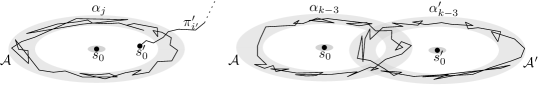
Figure 7: Two cases from the proof of Lemma 36.

We will now use use copies of $Q^{k}_{A}$ to construct $\varepsilon$-overlap graphs which will finish the proof.

Construction 34 ($H_{A}^{k}(G)$).

For any $G\in C(A)$, consider a fixed drawing of $G$ as a contact graph of $A$. For each vertex $w$ of $G$, we make a copy of the drawing of $Q_{A}^{k}$ as an intersection graph as defined in Construction 29 which we translate so that $s_{0}$ is placed at $s_{0}^{w}:=(2k-2)w$. We then add all edges induced by the vertices, and the result is denoted as $H_{A}^{k}(G)$.

To show that $H^{k}_{A}(G)$ does in fact construct $G$ as a $\varepsilon$-overlap graph, we need to show that if $ww^{\prime}$ is an edge of $G$, then the corresponding cycles $\alpha_{k}$ and $\alpha^{\prime}_{k}$ intersect each other. That implies the existence of vertices $v_{i}(k)$ and $v^{\prime}_{i^{\prime}}(k)$ of $\alpha_{k}$ and $\alpha^{\prime}_{k}$, respectively, such that $v_{i}(k)v^{\prime}_{i^{\prime}}(k)$ is an edge of $H_{A}^{k}(G)$.

Lemma 35.

Consider two vertices $w,w^{\prime}$ of a drawing of a graph $G$ as a contact graph. Denote by $Q$ and $Q^{\prime}$ the copies of $Q_{A}^{k}$ in $H_{A}^{k}(G)$ corresponding to $w$ and $w^{\prime}$, respectively, such that $s_{0},\pi_{i},\alpha_{j},v_{i}(j)$ denote objects in $Q$ and $s^{\prime}_{0},\pi^{\prime}_{i},\alpha^{\prime}_{j},v^{\prime}_{i}(j)$ denote objects in $Q^{\prime}$. If $v_{i}(j)v^{\prime}_{i^{\prime}}(j^{\prime})$ is an edge of $H_{A}^{k}(G)$, then $j+j^{\prime}\geq 2k-4$.

If $ww^{\prime}$ is an edge of $G$, then there is an edge $v_{i}(k)v_{i^{\prime}}^{\prime}(k)$ in $H_{A}^{k}(G)$.

Proof.

Assume that $j+j^{\prime}\leq 2k-3$. In the drawing of $H^{k}_{A}(G)$ as an intersection graph defined by Construction 34, we have

$$\left\|v_{i}(j)v^{\prime}_{i^{\prime}}(j^{\prime})\right\|_{A}\geq\left\|s_{0}s^{\prime}_{0}\right\|_{A}-\left\|s_{0}v_{i}(j)\right\|_{A}-\left\|s^{\prime}_{0}v^{\prime}_{i^{\prime}}(j^{\prime})\right\|_{A}=4k-4-2j-2j^{\prime}\geq 4>2,$$

so $v_{i}(j)v^{\prime}_{i^{\prime}}(j^{\prime})$ is not an edge of $H_{A}^{k}(G)$.

Suppose now that $ww^{\prime}$ is an edge of $G$. Let $\mathcal{A}:=\left\{x\in\mathbb{R}^{2}\;\middle|\;\left\|s_{0}x\right\|_{A}\in[2k-1,2k]\right\}$ be the annulus containing $\alpha_{k}$ (by Lemma 31) and $\mathcal{A}^{\prime}:=\left\{x\in\mathbb{R}^{2}\;\middle|\;\left\|s^{\prime}_{0}x\right\|_{A}\in[2k-1,2k]\right\}$ be that containing $\alpha^{\prime}_{k}$. The annuli $\mathcal{A}$ and $\mathcal{A}^{\prime}$ cross over each other as two Olympic rings (i.e., the difference $\mathcal{A}\setminus\mathcal{A}^{\prime}$ has two connected components). Lemma 33 then shows the intuitive fact that $\alpha_{k}$ and $\alpha^{\prime}_{k}$ must intersect. Therefore, there is an edge $v_{i}(k)v^{\prime}_{i^{\prime}}(k)$. ∎

We need one last fact before concluding that $H^{k}_{A}(G)$ constructs $G$ as an $\varepsilon$-overlap graph: for $X\in\{A,B\}$ and any two centers $s_{0},s^{\prime}_{0}$ of copies of $Q^{k}_{A}$, we have $\left\|s_{0}s^{\prime}_{0}\right\|_{X}=\Omega(k)$, and if the corresponding vertices $w,w^{\prime}$ share an edge in $G$, then $\left\|s_{0}s^{\prime}_{0}\right\|_{X}=O(k)$, as made precise in the following lemma.

Lemma 36.

Let $X\in\{A,B\}$ and $k\geq 7$. In the setting of Lemma 35, consider an arbitrary drawing of $H_{A}^{k}(G)$ as in intersection graph of $X$. Then $\left\|s_{0}s^{\prime}_{0}\right\|_{X}\geq 4k-18$ and if $ww^{\prime}$ is an edge of $G$, then $\left\|s_{0}s^{\prime}_{0}\right\|_{X}\leq 4k+2$.

Proof.

To prove the lower bound on $\left\|s_{0}s^{\prime}_{0}\right\|_{X}$, we show that $\left\|s_{0}s^{\prime}_{0}\right\|_{X}$ is neither in the interval $[0,k-7)$ nor in $[k-7,4k-18)$. The cases are depicted in Figure 7.

1. Suppose that $\left\|s_{0}s^{\prime}_{0}\right\|_{X}\in[0,k-7)$. Let $j:=\lceil\frac{k}{2}-2\rceil$. Then $s^{\prime}_{0}$ is in the ball $s_{0}+(2j-3)X$. By Lemma 32, $\alpha_{j}$ is contained in the annulus $\mathcal{A}:=\left\{x\in\mathbb{R}^{2}\;\middle|\;\left\|s_{0}x\right\|_{X}\in(2j-3,2j]\right\}$. Note that $\mathcal{A}$ has diameter $4j<2k-3$. It follows from Lemma 32 that any of the subpaths of $\pi^{\prime}_{i^{\prime}}$ from $s^{\prime}_{0}$ to $v^{\prime}_{i^{\prime}}(k)$ connects the inner and outer boundary of $\mathcal{A}$. Therefore, Lemma 33 gives that $\pi^{\prime}_{i^{\prime}}$ crosses $\alpha_{j}$. Thus, there is also an edge $v_{i}(j)v^{\prime}_{i^{\prime}}(j^{\prime})$ of $H_{A}^{k}(G)$, where $j+j^{\prime}\leq\lceil\frac{k}{2}-2\rceil+k<2k-4$, contradicting Lemma 35.

2. Suppose now that $\left\|s_{0}s^{\prime}_{0}\right\|_{X}\in[k-7,4k-18)$. By an argument similar to the one used in the proof of Lemma 35, one can show that $\alpha_{k-3}$ crosses $\alpha^{\prime}_{k-3}$. Hence, there is an edge $v_{i}(k-3)v^{\prime}_{i^{\prime}}(k-3)$, contradicting Lemma 35.

Consider now the case that $ww^{\prime}$ is an edge of $G$. By Lemma 35, we know that there is an edge $v_{i}(k)v^{\prime}_{i^{\prime}}(k)$. Then $\left\|s_{0}s^{\prime}_{0}\right\|_{X}\leq\left\|s_{0}v_{i}(k)\right\|_{X}+\left\|v_{i}(k)v^{\prime}_{i^{\prime}}(k)\right\|_{X}+\left\|v^{\prime}_{i^{\prime}}(k)s^{\prime}_{0}\right\|_{X}\leq 4k+2$. ∎

We are now ready to show that $H^{k}_{A}(G)$ does in fact construct $G$ as a $\varepsilon$-overlap graph.

Lemma 37.

For a graph $G=(V,E)\in C(A)$, if $H_{A}^{k}(G)\in I(B)$ for $k\geq 7$, then $G\in C_{10/k}(B)$.

Proof.

Suppose that $H_{A}^{k}(G)\in I(B)$ and consider a drawing of $H_{A}^{k}(G)$ as an intersection graph of $B$, and define $\mathcal{A}:=\left\{\frac{s_{0}^{u}}{2k+1}\;\middle|\;u\in V\right\}$. It follows directly from Lemma 36 that $I_{B}(\mathcal{A})$ is a drawing of $G$ as a $\left(2-\frac{4k-18}{2k+1}\right)$-overlap graph of $B$. Since $\frac{4k-18}{2k+1}\geq 2-10/k$, the statement follows. ∎

Theorem 3 is an easy consequence of Lemma 37 and Lemma 24:

Proof of Theorem 3.

Let $G=(V,E^{\prime})$ have the property from the theorem and suppose that $I(A)=I(B)$. Then in particular, $H_{A}^{k}(G)\in I(B)$ for all $k>0$. By Lemma 37 and 24, there is a graph $H=(V,E)\in C(B)$ such that $E^{\prime}\subseteq E$, which is a contradiction. ∎

References

- [1] Károly Böröczky Jr. Finite packing and covering, volume 154 of Cambridge Tracts in Mathematics. 2004.
- [2] Sergio Cabello and Miha Jejčič. Refining the hierarchies of classes of geometric intersection graphs. The Electronic Journal of Combinatorics, 24(1):1–19, 2017.
- [3] Jean Cardinal. Computational geometry column 62. SIGACT News, 46(4):69–78, 2015.
- [4] Jean Cardinal, Stefan Felsner, Tillmann Miltzow, Casey Tompkins, and Birgit Vogtenhuber. Intersection graphs of rays and grounded segments. In 43rd International Workshop on Graph-Theoretic Concepts in Computer Science (WG 2017), pages 153–166.
- [5] Steven Chaplick, Stefan Felsner, Udo Hoffmann, and Veit Wiechert. Grid intersection graphs and order dimension. Order, 35:363–391, 2018.
- [6] Adrian Dumitrescu and Minghui Jiang. Piercing translates and homothets of a convex body. Algorithmica, 61(1):94–115, 2011.
- [7] Adrian Dumitrescu and Minghui Jiang. Coloring translates and homothets of a convex body. Beiträge zur Algebra und Geometrie/Contributions to Algebra and Geometry, 53(2):365–377, 2012.
- [8] Gábor Fejes Tóth. New results in the theory of packing and covering. In Convexity and its Applications, pages 318–359. 1983.
- [9] László Fejes Tóth. Lagerungen in der Ebene auf der Kugel und im Raum, volume 65 of Die Grundlehren der mathematischen Wissenschaften. Second edition, 1972.
- [10] Stefan Felsner and Günter Rote. On primal-dual circle representations. In 34th European Workshop on Computational Geometry (EuroCG 2018), pages 72:1–72:6.
- [11] György Pál Gehér. A contribution to the aleksandrov conservative distance problem in two dimensions. Linear Algebra and its Applications, 481:280–287, 2015.
- [12] Svante Janson and Jan Kratochvíl. Thresholds for classes of intersection graphs. Discrete Mathematics, 108:307–326, 1992.
- [13] Seog-Jin Kim, Alexandr Kostochka, and Kittikorn Nakprasit. On the chromatic number of intersection graphs of convex sets in the plane. the electronic journal of combinatorics, 11(1):52, 2004.
- [14] Seog-Jin Kim and Kittikorn Nakprasit. Coloring the complements of intersection graphs of geometric figures. Discrete Mathematics, 308(20):4589–4594, 2008.
- [15] Seog-Jin Kim, Kittikorn Nakprasit, Michael J. Pelsmajer, and Jozef Skokan. Transversal numbers of translates of a convex body. Discrete Mathematics, 306(18):2166–2173, 2006.
- [16] P. Koebe. Kontaktprobleme der konformen Abbildung. Berichte über die Verhandlungen der Sächsische Akademie der Wissenschaften zu Leipzig, Mathematisch–Physische Klasse, 88:141–164, 1936.
- [17] Jan Kratochivíl and Jiří Matoušek. Intersection graphs of segments. Journal of Combinatorial Theory Series B, 62(2):289–315, 1994.
- [18] Colin McDiarmid and Tobias Müller. Integer realizations of disk and segment graphs. Journal of Combinatorial Theory, Series B, 103(1):114–143, 2013.
- [19] Tobias Müller, Erik Jan van Leeuwen, and Jan van Leeuwen. Integer representations of convex polygon intersection graphs. SIAM Journal on Discrete Mathematics, 27(1):205–231, 2013.
- [20] Irina G. Perepelitsa. Bounds on the chromatic number of intersection graphs of sets in the plane. Discrete Mathematics, 262:221–227, 2003.
- [21] Oded Schramm. Combinatorically prescribed packings and applications to conformal and quasiconformal maps. Preprint, \urlhttps://arxiv.org/abs/0709.0710, 2007.
- [22] Konrad Swanepoel. Combinatorial distance geometry in normed spaces. In Gergely Ambrus, Imre Bárány, Károly J. Böröczky, Gábor Fejes Tóth, and János Pach, editors, New Trends in Intuitive Geometry, volume 27 of Bolyai Society Mathematical Studies.