6D Object Pose Estimation without PnP

Abstract

In this paper, we propose an efficient end-to-end algorithm to tackle the problem of estimating the 6D pose of objects from a single RGB image. Our system trains a fully convolutional network to regress the 3D rotation and the 3D translation in region layer. On this basis, a special layer, Collinear Equation Layer, is added next to region layer to output the 2D projections of the 3D bounding boxs corners. In the back propagation stage, the 6D pose network are adjusted according to the error of the 2D projections. In the detection phase, we directly output the position and pose through the region layer. Besides, we introduce a novel and concise representation of 3D rotation to make the regression more precise and easier. Experiments show that our method outperforms base-line and state of the art methods both at accuracy and efficiency. In the LineMod dataset, our algorithm achieves less than 18 ms/object on a GeForce GTX 1080Ti GPU, while the translational error and rotational error are less than 1.67 cm and 2.5 degree.

1 Introduction

Object detection and localization has always been a hot topic of computer vision. Traditional methods, like YOLO[1], SSD[2] and Mask R-CNN[3], have experienced a tremendous success in 2D domain. However, those methods cant achieve accurate semantic understanding of the objective three-dimensional world. The ultimate goal of computer vision is to study the nature of the objective threedimensional world through images. To tackle this, more and more attention has been paid to object 6D pose estimation. Real-time 6D pose estimation is crucial for augmented reality, virtual reality and robotics.

Currently, feature-based methods[4,5,6], template-based methods[7,8] and RGB-D methods[9,10,11,12,13] have achieved robust results to some extent. Feature-based methods tackled this task by matching feature points between 3D models and images. However, only when there are rich textures on the objects that those methods work. As a result, they are unable to handle texture-less objects[14]. Template-based methods use a rigid template to match different locations in the input image. Such methods are likely to be affected by occlusions. RGB-D methods use depth data as additional information, which simplifies the task. However, active depth sensors are power hungry, which makes 6D objective detection methods for passive RGB images more attractive for mobile and wearable cameras[15]. Besides, acquiring depth data needs additional hardware costs.

Deep learning techniques have recently become mainstream to estimate 6D object pose, among which [15] and [21] are two typical examples. In [15, 21], CNNs are used to predict 2D projections of 3D bounding boxs corners (for the sake of simplification, we call the 2D projections pts), then 6D pose are obtained by PnP algorithm. The deficiency of the two methods is that PnP costs extra time, decreasing the efficiency. In this paper, we propose a generic framework which overcomes the shortcomings of existing methods to estimate 6D object pose. We extend YOLO V2[26] to perform 6D pose estimation from single RGB images. In the training phase, we feed images to the fully convolutional channels to output the 3D translation parameters (tu, tv, tw) and 3D rotation parameters (a, b, c). The special layer, Collinear Equation Layer, follows the meta-architecture of YOLO with architecture adaptation and tuning to predict the pts. Then we adjust the network with the pts error. Unlike [15] and [21], in the testing phase, we discard Collinear Equation Layer and directly predict 6D pose parameters.

Our work has the following advantages and contributions:

a) We propose a novel method for 6D pose estimation in a really end-to-end manner. We bring in Collinear Equation Layer to regress 2D projections of 3D bounding boxs corners to train our network. In the testing stage, we discard the last layer and directly obtain 6D pose, avoiding PnP algorithm, which makes the estimation fast and accurate.

b) We introduce a brand new representation for 3D rotation. This representation is easy to regression.

c) Extending YOLO V2 to directly predict 6D pose.

The remainder of the paper is organized as follows. After the overview of related work, we introduce our method.Then we display the experimental results, followed by the final conclusion.

2 Related Work

The literature on 6D pose estimation is very large and we have mentioned some in the previous section, thus we will focus only on recent works based on deep learning. Most of recent works use CNN to solve 6D pose problems, including camera pose[16, 17] and object pose[15,18,19,20,21,22,23,24].

In [16,17], the authors train CNNs to directly regress 6D camera pose from a single RGB image. The camera pose estimation is much easier than the object pose estimation, for there is no need to detect any object.

In [18,19], the authors use CNNs to regress 3D object pose directly, their works focus only on 3D rotation estimation while 3D translation is not included. In [20], SSD detection framework is extended to 6D pose estimation. The authors transform pose detection into two-stage classification tasks, view angle classification and in-plane rotation classification. However, wrong classification in either stage could cause an incorrect pose estimation. In [22], the authors first use a CNN to regress 3D object orientation, then combines these estimates with geometric constraints provided by a 2D object bounding box to produce a complete 3D bounding box. However, in general, this method needs to solve 4096 linear equations. In special circumstances, such as the KITTI dataset[25], object pitch and roll angles are both zero, there are still 64 equations to be solve, which makes the method computational costly. In [23], the pose parameters are decoupled into translation and rotation, then the rotation is regressed via a Lie algebra representation. This method assumes that the 2D projection of the objects origin is in the 2D boxs center, which makes the estimation of translation inaccuracy. In [24], a feedback loop consisting of deep networks are developed for 6D pose estimation. In this method, the inaccurate pose data is re-projected and compared with the original image for accurate correction. However, the preparation of sample is intricate.

BB8[21] provides a precise method to estimation 6D pose. the authors firstly use a segmentation network to localize objects. Then another CNN is used to predict the 2D projections of the 3D bounding boxs corners around the object. The 6D pose is estimated through a PnP algorithm. Finally, a CNN is trained to refine the pose. The method is multi-stage, which increases their running time. Similar to BB8, [15] detects the 2D projections of the corners, too. But the authors use a direct way by propose a singleshot deep CNN architecture, then employ PnP algorithm to get the 6D pose. Both [21] and [15] achieve high accuracy. However, the two method employ PnP algorithm to attain 6D pose, which is not really end-to-end, and the PnP algorithm will cost extra time. Besides, the regression of each corner is independent and no constraint exists. This may result in that some corners are inaccurately predicted, which will have bad impact on the PnP algorithm. Compared to them, our method regresses the corners with constraint produced by Collinearity Equation Layer in the training stage, but directly predict 6D pose while testing. In this way, we avoid the shortcomings raised by PnP.

3 Method

3.1 Position parameter

According to the small hole imaging equation we have the following formula:

$$\begin{split}{{t}}&={{z}}{K^{-1}}\left[{\begin{array}[]{*{20}{c}}u\\ v\\ 1\end{array}}\right]\\ &={\rm{z}}{K^{-1}}\left[{\begin{array}[]{*{20}{c}}{W({c_{0}}+0.5+\Delta u)/w}\\ {H\left({{r_{0}}+0.5+\Delta v}\right)/h}\\ 1\end{array}}\right]\end{split}$$ (1)

considering

$${K^{-1}}=\left[{\begin{array}[]{*{20}{c}}{\frac{1}{{{f_{x}}}}}&0&{-\frac{{{c_{x}}}}{{{f_{x}}}}}\\ 0&{\frac{1}{{{f_{y}}}}}&{-\frac{{{c_{y}}}}{{{f_{y}}}}}\\ 0&0&1\end{array}}\right]$$ (2)

we get

$${\bf{t}}={\bf{b}}{{\bf{e}}^{tw}}\left[{\begin{array}[]{*{20}{c}}{\frac{1}{{{{\bf{f}}_{x}}}}\left({\frac{{W({c_{0}}+0.5+s\sigma\left({{t_{u}}}\right))}}{w}-{c_{x}}}\right)}\\ {\frac{1}{{{{\bf{f}}_{y}}}}\left({\frac{{H({r_{0}}+0.5+s\sigma\left({{t_{v}}}\right))}}{h}-{c_{y}}}\right)}\\ 1\end{array}}\right]$$ (3)

where $\sigma(.)$ is the loggy excitation function and s is an adjustable parameter. Considering that the object may be distributed over a large range, we take s=4.0. The neural network outputs three translation variables tu, tv, tw $\rightarrow$ [$\Delta$u, $\Delta$v, z]$\rightarrow$[X Y Z]=t.

3.2 Pose parameter

The rotation matrix R in the collinear equation can perfectly express the rotation of the camera relative to the object. However, the R matrix is not suitable for direct prediction using neural networks. Because R is a unit orthogonal matrix, there are too many redundancy, so we use abc conversion:

$$\begin{split}R&=\frac{1}{{1+{a^{2}}+{b^{2}}+{c^{2}}}}\\ &\left[\!\!\!\!{\begin{array}[]{*{20}{c}}{1+{a^{2}}-{b^{2}}-{c^{2}}}&{2ab-2c}&{2ac+2b}\\ {2ab+2c}&{1-{a^{2}}+{b^{2}}-{c^{2}}}&{2bc-2a}\\ {2ac-2b}&{2bc+2a}&{1-{a^{2}}-{b^{2}}+{c^{2}}}\end{array}}\!\!\!\!\right]\end{split}$$ (4)

The abc can be predicted by the neural network and then the (4) equation can be used to obtain the pose matrix. The abc transform does not need to worry about the angle loop problem, and there is no redundancy without worrying about the unitized constraint problem. Therefore, the abc is selected for network pose prediction.

3.3 Overall pipeline

The main idea of this paper is to propose a full convolution network that implements 6DPose. This idea is to add a collinear equation layer after the region layer of the deep network. In the training phase, the region layer predicts the position and rotation parameters R and t. The coordinates u, v are backpropagated by regression 2D pts to correct R and t. In the prediction phase, R and t are directly obtained by the region layer. Figure 1 shows the pipeline.

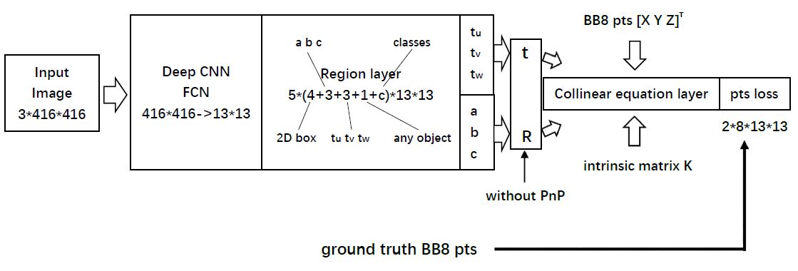
Figure 1: Overall pipeline.

The input of the neural network is a 3*416*416 color image, which are converted into a 13*13 array through a full convolutional network, and output 5*(4+3+3+1+c) channels through a 13x13 arrays region layer, in which 4 channels record 2D box coordinate information, three channels abc record rotation data, three channels tu,tv,tw are responsible for 3d translation. one channel is responsible for whether the object is near the cell, c channel softmax outputs the target category.

In order to improve the detection accuracy, we have designed five anchors with reference to yolov2, which are used to extract objects of different scales.

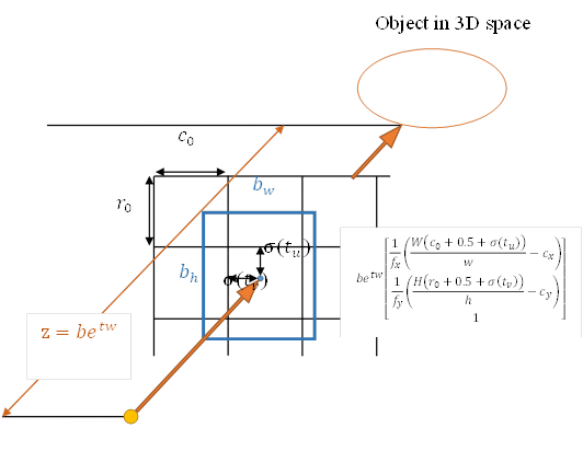
Figure 2: Schematic diagram of the 3D position prediction of the region layer.

4 Collinear Equation Layer

As shown in Fig.1, The Collinear Equation Layer is responsible for adjusting the position and rotation parameters by pts error back propagation.

4.1 Forward propagation

$$z\left[{\begin{array}[]{*{20}{c}}u\\ v\\ 1\end{array}}\right]=KR\left({X-T}\right)=K\left({RX+t}\right)$$ (5)

The last layer in Figure 1 is a mapping operation that implements small hole imaging. Divide the first line of equation (5) by the third line, and divide the second line by the third line to get the collinear equation as follows:

$$\left\{\begin{array}[]{l}u={c_{x}}+{f_{x}}\frac{X}{Z}={c_{x}}+{f_{x}}\frac{{{r_{11}}{X_{x}}+{r_{12}}{X_{y}}+{r_{13}}{X_{z}}+{{\rm{t}}_{x}}}}{{{r_{31}}{X_{x}}+{r_{32}}{X_{y}}+{r_{33}}{X_{z}}+{t_{z}}}}\\ v={c_{y}}+{f_{y}}\frac{Y}{Z}={c_{y}}+{f_{y}}\frac{{{r_{21}}{X_{x}}+{r_{22}}{X_{y}}+{r_{23}}{X_{z}}+{t_{y}}}}{{{r_{31}}{X_{x}}+{r_{32}}{X_{y}}+{r_{33}}{X_{z}}+{t_{z}}}}\end{array}\right\}$$ (6)

Among them, $\text{r}_{11}$-$\text{r}_{33}$ are the 9 elements of the unit orthogonal matrix R, which can be expressed by abc in Eq.(4).The formula (6) can be regarded as the forward propagation formula of the collinear equation layer. Where R is obtained by abc output from the neural network region layer through the formula (4), and t is obtained by the formula (3).

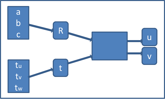
Figure 3: Forward propagation calculation process

4.2 Backward propagation

The collinear equation layer is only used during the training phase in order to pass the error of the pts to the 6D pose parameters in region layer error, so that the error weights of the R and t parameters can be reasonably allocated. Defined according to the definition of error:

$$loss{\rm{}}={\rm{}}{\rm{|pt}}{{\rm{s}}_{predict}}-(\overline{pts}){|_{2}}$$ (7)

$$\frac{{\partial E_{qt}^{2}}}{{\partial u}}=\mathop{\sum}\limits_{i=1}^{n}{\left({{\rm{ui}}-\overline{{\rm{ui}}}}\right)^{2}}$$ (8)

$$\frac{{\partial E_{qt}^{2}}}{{\partial v}}=\mathop{\sum}\limits_{i=1}^{n}{\left({{\rm{vi}}-\overline{{\rm{vi}}}}\right)^{2}}$$ (9)

Where n is the number of pts points. The figure below shows the backward propagation process.

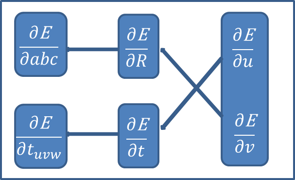
Figure 4: Collinear equation layer backward propagation process

5 Overall network structure

5.1 Network Design

In Figure 1, DeepCNN is a mapping from 3*416*416 to 13*13*5*(4+3+3+1+c). We designed two fully convolutional networks for 6DPose prediction. Network 6D Pose-linemod-13c for 3D mesh ply dataset for LineMod[7]. Network 6D Pose-voc-8c for 8 typical objects in the VOC2007+VOC2012 dataset.

In network 6DPose-linemode-13c, we design a c=13 category object for linemode 3DMesh, conv layer29 output 5*(11+13)=120 channels.

layer	filters	size	input	output
0 conv	32	3*3/1	416*416*3	416*416*32
1 max		2*2/2	416*416*32	208*208*32
2 conv	64	3*3/1	208*208*32	208*208*64
3 max		2*2/2	208*208*64	104*104*64
4 conv	128	3*3/1	104*104*64	104*104*128
5 conv	64	1*1/1	104*104*128	104*104*64
6 conv	128	3*3/1	104*104*64	104*104*128
7 max		2*2/2	104*104*128	52*52*128
8 conv	256	3*3/1	52*52*128	52*52*256
9 conv	128	1*1/1	52*52*256	52*52*128
10 conv	256	3*3/1	52*52*128	52*52*256
11 max		2*2/2	52*52*256	26*26*256
12 conv	512	3*3/1	26*26*256	26*26*512
13 conv	256	1*1/1	26*26*512	26*26*256
14 conv	512	3*3/1	26*26*256	26*26*512
15 conv	256	1*1/1	26*26*512	26*26*256
16 conv	512	3*3/1	26*26*256	26*26*512
17 max		2*2/2	26*26*512	13*13*512
18 conv	1024	3*3/1	13*13*512	13*13*1024
19 conv	512	1*1/1	13*13*1024	13*13*512
20 conv	1024	3*3/1	13*13*512	13*13*1024
21 conv	512	1*1/1	13*13*1024	13*13*512
22 conv	1024	3*3/1	13*13*512	13*13*1024
23 conv	1024	3*3/1	13*13*1024	13*13*1024
24 conv	1024	3*3/1	13*13*1024	13*13*1024
25 route	16
26 reorg		/2	26*26*512	13*13*2048
27 route	26	24
28 conv	1024	3*3/1	13*13*3072	13*13*1024
29 conv	220	1*1/1	13*13*1024	13*13*120
30 region				13*13*5*(4+3+3+1+13)

Table 1: Structure of network 6DPose-linemode-13c

5.2 3D mesh sample training and augmentation

3D augmentation is implemented using the document and the OpenGL rendering algorithm described in [20].

5.3 VOC 2D image sample training and augmentation

We have built a VOC3D dataset. In order to improve the labeling speed, we use the mouse to pull out the XYZ three axes on the image to determine the target’s posture R=r11,…,r33. Suppose the user uses the mouse to mark the axis vector dx, dy, dz direction of the object on the image, and the linear equation au+bv+c=0 on the corresponding image satisfies the equation below:

$$\left[{\begin{array}[]{*{20}{c}}a&b&c\end{array}}\right]KR\left[{\begin{array}[]{*{20}{c}}{{d_{x}}}\\ {{d_{y}}}\\ {{d_{z}}}\end{array}}\right]=0$$ (10)

That is, the rotation R is the solution of equation (10). The rotation data R can be solved by using the LM algorithm. Translation T is the solution to the equation below:

$$\begin{split}&\left[{\tiny\begin{array}[]{*{20}{c}}{{u_{KiL}}{r_{31}}-{r_{11}}}&{{u_{KiL}}{r_{32}}-{r_{12}}}&{{u_{KiL}}{r_{33}}-{r_{13}}}\\ {{u_{KiR}}{r_{31}}-{r_{11}}}&{{u_{KiR}}{r_{32}}-{r_{12}}}&{{u_{KiR}}{r_{33}}-{r_{13}}}\\ {{v_{KiT}}{r_{31}}-{r_{21}}}&{{v_{KiT}}{r_{32}}-{r_{22}}}&{{v_{KiT}}{r_{33}}-{r_{23}}}\\ {{v_{KiB}}{r_{31}}-{r_{21}}}&{{u_{KiB}}{r_{32}}-{r_{22}}}&{{v_{KiB}}{r_{33}}-{r_{23}}}\end{array}}\right]{\small\rm{T}}\!\!=\!\!\\ \ &\begin{bmatrix}\!\!\!\!\!\!\!\!\begin{smallmatrix}\begin{smallmatrix}\begin{smallmatrix}\begin{smallmatrix}{\tiny\begin{array}[]{*{20}{c}}{\left({{u_{KiL}}{r_{31}}-{r_{11}}}\right){x_{iL}}+\left({{u_{KiL}}{r_{32}}-{r_{12}}}\right){y_{iL}}+\left({{u_{KiL}}{r_{33}}-{r_{13}}}\right){z_{iL}}}\\ {\left({{u_{KiR}}{r_{31}}-{r_{11}}}\right){x_{iR}}+\left({{u_{KiR}}{r_{32}}-{r_{12}}}\right){y_{iR}}+\left({{u_{KiR}}{r_{33}}-{r_{13}}}\right){z_{iR}}}\\ {\left({{v_{KiT}}{r_{31}}-{r_{21}}}\right){x_{iT}}+\left({{u_{KiT}}{r_{32}}-{r_{22}}}\right){y_{iT}}+\left({{u_{KiT}}{r_{33}}-{r_{23}}}\right){z_{iT}}}\\ {\left({{v_{KiB}}{r_{31}}-{r_{21}}}\right){x_{iB}}+\left({{u_{KiB}}{r_{32}}-{r_{22}}}\right){y_{iB}}+\left({{u_{KiB}}{r_{33}}-{r_{23}}}\right){z_{iB}}}\end{array}}\end{smallmatrix}\end{smallmatrix}\end{smallmatrix}\end{smallmatrix}\!\!\!\!\!\!\!\!\end{bmatrix}\!\!\!\!\end{split}$$ (11)

Thus, we can obtain the displacement data t of the labeled data only by solving only one linear equation. According to the pose data and the three values of the length, width and height of the target, 8 virtual feature point coordinates of the target can be obtained as the training data of our algorithm. The 2DImage data augmentation uses the affine transformation to perform a proportional translation, scaling and rotation transformation of the image and the virtual feature point coordinate synchronization.

We selected 8 types of objects suitable for 6DPose from 20 categories of objects in VOC2007 and VOC2012 to create a small VOC3d data set as follows: aero plane, boat, bus, car, chair, motorbike, person, tv monitor.

According to the discussion in Sec.5.1, the output of the last layer of the fully convolutional network is 13*13, 5*(11+c) channel data, where c=8, and the region layer accesses 95 from the 29 conv layer.

From the VOC tag image, 500 image samples were taken for testing, and the remaining 6538 images were used for training. 6D Pose prediction is shown in next section.

6 Experiments

As described in Sec.5.1, we constructed two networks to train 3D mesh file recognition for linemode and 2D image data for VOC2007 and VOC2012, and then predict 6D Pose for the trained model. We then evaluated the accuracy and speed of 6DPose prediction.

6.1 Evaluation for LineMod dataset

Firstly, we use the object.xyz file in linemode to train the linemode-6DPose-c13 model. The linemode gives the rot file and the tra file corresponding to the target’s pose and translation GroundTruth values. The 6DPose prediction projection cube and the GroundTruth projection cube are overlapping displayed as follows:

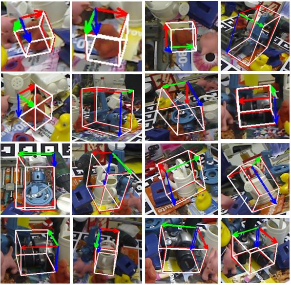
Figure 5: LineMod object 6D pose prediction demo, overlapping displayed.

The white box in Figure 5 is the GroundTruth object cube, and the red+green+blue cube is the projection corresponding to the network predicted R-t, and the two Cubes can basically overlap. The direction of the red arrow is the positive X-axis of the object itself, the direction of the green arrow is the positive direction of the Y-axis, and the direction of the blue arrow is the positive direction of the Z-axis. To evaluate our method and compare it with state of the art method, we use two metrics, 2D projection error[30] and rotational and translational error[31].

Object	Average pixel projection error	5 pixels accuracy	5 pixels accuracy	5 pixels accuracy
	Our method	Ours	SS6D[27]	BB8[21]
ape	1.98	0.9894	0.9210	0.9530
cam	2.64	0.9658	0.9324	0.809
glue	2.67	0.9680	0.9653	0.890
box	2.54	0.9457	0.9033	0.879
can	3.17	0.9130	0.9744	0.841
lamp	2.50	0.9347	0.7687	0.744
bench	4.25	0.7152	0.9506	0.800
cat	2.53	0.9826	0.9741	0.970
hole	2.61	0.9352	0.9286	0.905
duck	2.58	0.9534	0.9465	0.812
iron	2.52	0.9015	0.8294	0.789
driller	2.60	0.8985	0.7941	0.7941
phone	2.69	0.9458	0.8607	0.776
average	2.71	0.9268	0.9037	0.839
bowl	2.67	0.9562
cup	2.98	0.9325

Table 2: State of the art comparison of our method against SS6D and BB8 using 2D projection error.As in [28], we use the percentage of correctly predicted poses for each object. A pose is considered correct if the 2D projection pixel error is less than 5 pixels. The second column is the average pixel porjection error of our method. The last three columns are the comparison of our method against the state of art methods in 5 pixels manner.

Object	ours($\text{e}_{TE}$)	BB8($\text{e}_{TE}$)	ours($\text{e}_{RE}$)	BB8($\text{e}_{RE}$)
ape	1.88	1.85	2.45	2.54
cam	1.85	1.89	2.43	2.55
glue	1.67	1.98	2.51	2.38
box	1.54	1.78	2.10	2.40
can	1.80	1.97	2.38	2.13
lamp	1.50	1.67	2.26	2.10
bench	1.82	1.78	3.03	2.83
cat	1.53	1.56	2.25	2.43
hole	1.61	1.65	2.31	2.76
duck	1.58	1.72	2.65	2.53
iron	1.52	1.55	2.59	2.94
driller	1.60	1.66	2.34	2.39
phone	1.69	1.70	2.29	2.41
average	1.66	1.75	2.43	2.49

Table 3: State of the art comparison of our method against BB8 using rotational and translational error. The unit of $\text{e}_{TE}$ and $\text{e}_{RE}$ are cm and degree.

From the above two tables, the performance of our method is better than that of BB8 and SS6D on both 2D project and 6D pose accuracy evaluation criteria.

Experiments have found that for the BB8 algorithm, each pts is completely independent, and the error is determined by the max pts error of pts. For our Direct 6D Pose, pts is preceded by collinear equations, and the algorithm error depends on the overall error of pts. Therefore, Direct 6DPose is very suitable for stereo vision position and rotation prediction.

6.2 Evaluation for VOC3D 2D images

The prediction effect of the 6D pose-voc-8c network designed by Sec.5.3 for predicting 8 typical VOC targets is shown in Figure 6. The average pixel projection error (pixels) for 6D pose-voc-8c prediction is shown in Table 4.

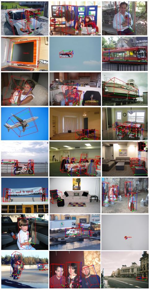
Figure 6: 6D pose predicted by the 6D pose-voc-c8 network.

Object	error(8pts)	error(27pts)
airplane	8.38	6.26
boat	9.89	8.65
bus	11.10	7.67
car	9.45	8.54
chair	8.47	6.35
motorbike	6.50	5.18
person	9.25	8.93
tv monitor	9.53	8.78

Table 4: Average pixel projection error (pixels) for 6D pose-voc-8c prediction

The cause of the error: 1. The internal parameters of the camera are not accurate; 2. Without accurate point cloud data, the length, width and height of the object are not always accurate, but if the length, width and height ratio are correct, the projected coordinates of the object on the image can still be correct.

The 6D pose R-t predicted by the network is used to draw the effect of the 3D object Cube on the image. The red arrow is the target’s own X axis, and the green arrow is the target Y axis, the blue arrow is the target’s Z axis. This 6Dose 2DProject error predicted by 6DPose-voc-8c is within the acceptable range of visual inspection.

6.3 Computation times

Our implementation takes 16-17ms for one object 6D pose prediction, on an Intel Core i7-5820K 3.30 GHz desktop with a GeForce 1080Ti. The table below shows the computation times comparsions between our method and other methods.

Method	computation time (ms)
SSD-6D	20
BB8	130
Brachmann et al.	500
Rad and Lepetit	333
6D pose-linemode-13c	18
6D pose-voc-8c	17

Table 5: Computation time comparison.

7 Conclusion

We designed an end-to-end 6D pose network which used the advantages of BB8 pts regression, but propagated the pts error back to the position and attitude error through the collinear equation layer, thus avoiding the post-processing pnp processing. In this way, the implementation consumption and additional errors caused by the Pnp algorithm are avoided. This algorithm can achieve 55 fps, the average 6dpose 5-pixel projection error is 0.928, the average translation error is less than 1.7cm, and the average rotation error is lessthan 2.5 degree. The algorithm does not require refinement or other post-processing post-processing. In the future, we will further extend the training data set from VOC data to COCO to achieve 6D pose prediction of large-scale 2D image data, so that 6D pose technology can be more practical for outdoor large-scale natural scenes.

8 Acknowledgement

This research was supported by Wuhan Xiongchugaojing Tech Company. We gratefully acknowledge the support of Wuhan Xiongchugaojing Tech Company with the donation of the GTX 1080Ti GPU used for this research.

References

- [1] Redmon J, Divvala S, Girshick R, et al. You Only Look Once: Unified, Real-Time Object Detection. In CVPR, 2016.
- [2] W. Liu, D. Anguelov, D. Erhan, C. Szegedy, S. Reed, C. Fu, and A. C. Berg. SSD: Single Shot MultiBox Detector. In ECCV, 2016.
- [3] K. He, G. Gkioxari , P. Dollar, et al. Mask R-CNN. In TPAMI, 2017.
- [4] A. Collet, M. Martinez, and S. S. Srinivasa. The MOPED framework: Object recognition and pose estimation for manipulation. In IJRR, 2011.
- [5] D. G. Lowe. Object recognition from local scaleinvariant features. In ICCV, 1999.
- [6] F. Rothganger, S. Lazebnik, C. Schmid,and J. Ponce. 3D object modeling and recognition using local affine-invariant image descriptors and multiview spatial constraints. In IJCV, 2006.
- [7] S. Hinterstoisser, C. Cagniart, S. Ilic, P. Sturm, N. Navab, P. Fua, and V. Lepetit. Gradient Response Maps for Real-Time Detection of Texture-less Objects. In TPAMI, 2012.
- [8] S. Hinterstoisser, V. Lepetit, S. Ilic, S. Holzer, G. Bradski, K. Konolige, and N. Navab. Model Based Training, Detection and Pose Estimation of Texture-Less 3D Objects in Heavily Cluttered Scenes. In ACCV, 2012.
- [9] E. Brachmann, A. Krull, F. Michel, S. Gumhold, J. Shotton, and C. Rother. Learning 6D Object Pose Estimation Using 3D Object Coordinates. In ECCV, 2014.
- [10] C. Choi and H. I. Christensen. 3D Textureless Object Detection and Tracking: An Edge-Based Approach. In IROS, 2012.
- [11] C. Choi and H. I. Christensen. RGB-D Object Pose Estimation in Unstructured Environments. In Robotics and Autonomous Systems, 2016.
- [12] W. Kehl, F. Milletari, F. Tombari, S. Ilic, and N. Navab. Deep Learning of Local RGB-D Patches for 3D Object Detection and 6D Pose Estimation. In ECCV, 2016.
- [13] K. Lai, L. Bo, X. Ren, and D. Fox. A Large-Scale Hierarchical Multi-View RGB-D Object Dataset. In ICRA, 2011.
- [14] Y. Xiang, T. Schmidt, V. Narayanan and D. Fox. PoseCNN: A Convolutional Neural Network for 6D Object Pose Estimation in Cluttered Scenes. arXiv preprint arXiv:1711.00199,, 2017.
- [15] B. Tekin, S. Sinha, and P. Fua. Real-Time Seamless Single Shot 6D Object Pose Prediction. arXiv preprint arXiv:1711.08848, 2017.
- [16] A. Kendall, M. Grimes, and R. Cipolla. PoseNet: A convolutional network for real-time 6-dof camera relocalization. In ICCV, 2015.
- [17] A. Kendall and R. Cipolla. Geometric loss functions for camera pose regression with deep learning. In CVPR, 2017.
- [18] S. Mahendran, H. Ali, and R. Vidal. 3D Pose Regression using Convolutional Neural Networks. In CVPR, 2017.
- [19] A. Doumanoglou, V. Balntas, R. Kouskouridas, and T. K. Kim. Siamese Regression Networks with Efficient mid-level Feature Extraction for 3D Object Pose Estimation. In NIPS, 2016.
- [20] Wadim Kehl, Fabian Manhardt, Federico Tombari, Slobodan Ilic, and Nassir Navab. SSD-6D: making rgbbased 3D detection and 6D pose estimation great again. In ICCV, 2017.
- [21] M. Rad and V. Lepetit. BB8: A scalable, accurate, robust to partial occlusion method for predicting the 3D poses of challenging objects without using depth. In ICCV, 2017.
- [22] A. Mousavian, D. Anguelov, J. Flynn, and J. Košecká. 3D Bounding Box Estimation using Deep Learning and Geometry. In CVPR, 2017.
- [23] T T. Do, M. Cai, T. Pham. Deep-6DPose: Recovering 6D Object Pose from a Single RGB Image. arXiv preprint arXiv:1802.10367, 2018.
- [24] M. Oberweger , P. Wohlhart , and V. Lepetit. Training a Feedback Loop for Hand Pose Estimation. In ICCV, 2015.
- [25] A. Geiger, P. Lenz, C. Stiller, and R. Urtasun. Vision meets robotics: The KITTI dataset. In IJRR, 2013.
- [26] S. Mahendran, H. Ali, and R. Vidal. 3D Pose Regression using Convolutional Neural Networks. In CVPR, 2017.
- [27] W. Kehl, F. Manhardt, F. Tombari, et al. SSD-6D: making rgbbased 3D detection and 6D pose estimation great again. In ICCV, 2017.
- [28] E. Brachmann, F. Michel, A. Krull, M. M. Yang,S. Gumhold, and C. Rother. Uncertainty-Driven 6D Pose Estimation of Objects and Scenes from a Single RGB Image. In CVPR, 2016.