Discovering bursts revisited:
guaranteed optimization of the model parameters

Abstract

One of the classic data mining tasks is to discover bursts, time intervals, where events occur at abnormally high rate. In this paper we revisit Kleinberg’s seminal work, where bursts are discovered by using exponential distribution with a varying rate parameter: the regions where it is more advantageous to set the rate higher are deemed bursty. The model depends on two parameters, the initial rate and the change rate. The initial rate, that is, the rate that is used when there are no burstiness was set to the average rate over the whole sequence. The change rate is provided by the user.

We argue that these choices are suboptimal: it leads to worse likelihood, and may lead to missing some existing bursts. We propose an alternative problem setting, where the model parameters are selected by optimizing the likelihood of the model. While this tweak is trivial from the problem definition point of view, this changes the optimization problem greatly. To solve the problem in practice, we propose efficient ($1+\epsilon$) approximation schemes. Finally, we demonstrate empirically that with this setting we are able to discover bursts that would have otherwise be undetected.

1 Introduction

Many natural phenomena occur unevenly over time, and one of the classic data mining tasks is to discover bursts, time intervals, where events occur at abnormally high rate. In this paper we revisit a seminal work by Kleinberg [13] that has been used, for example, in discovering trends in citation literature [3], analyzing topics [17], recommending citations [10], analyzing disasters [4], and analyzing social networks [1] and blogs [15].

Kleinberg [13] discovers bursts by modelling the time between events with an exponential model with varying rate parameter. The rate starts at the base level $\beta$ and can be raised (multiple times) by a change parameter $\alpha$, but it cannot descend $\beta$. Every time we raise the parameter, we need to pay a penalty. In the original approach, the change rate $\alpha$ is given as a parameter and the base rate is selected to be $\beta=1/\mu$, where $\mu$ is the average of the sequence.

We argue that this choice of $\beta$ is suboptimal: (i) it does not maximize the likelihood of the model, and, more importantly, (ii) a more optimized $\beta$ may reveal bursts that would have gone undetected.

We propose a variant of the original burstiness problem, where we are no longer given the base parameter $\beta$ but instead we are asked to optimize it along with discovering bursts. We also consider variants where we optimize $\alpha$ as well. These tweaks are rather mundane from the problem definition point of view but it leads to a surprisingly difficult optimization problem.

We consider two different models for the delays: exponential and geometric. First, we will show that we can solve our problem for exponential model in polynomial time, when $\alpha$ is given. Unfortunately, this algorithm requires $\mathit{\mathcal{O}}\mathopen{}\left(n^{3}k^{4}\right)$ time,​ thus being impractical. Even worse, we cannot apply the same approach for geometric model. This is a stark contrast to the original approach, where the computational complexity is $\mathit{\mathcal{O}}\mathopen{}\left(nk\right)$.

Fortunately, we can estimate burst discovery in quasi-linear time w.r.t. the sequence length; see Table 1 for a summary of the algorithms. We obtain $(1+\epsilon)$ approximation guarantee for the geometric model. We also obtain, under some mild conditions, $(1+\epsilon)$ approximation guarantee for the exponential model.

In all four cases, the algorithm is simple: we test multiple values of $\beta$ (and $\alpha$), and use the same efficient dynamic program that is used to solve the original problem. Among the tested sequences we select the best one. The main technical challenge is to test the multiple values of $\alpha$ and $\beta$ such that we obtain the needed guarantee while still maintaining a quasi-linear running time with respect to sequence length.

The remainder of the paper is as follows. We review the original burstiness problem in Section 2, and define our variant in Section 3. We introduce the exact algorithm in Section 4, and present the approximation algorithms in Section 5–6. In Section 7, we present the related work. In Section 8, we compare demonstrate empirically that our approach discovers busts that may go unnoticed. We conclude with discussion in Section 9. The proofs are given in Appendix, available in the full version of this paper.

Table 1: Summary of algorithms discussed in this paper. Here $k$ is the number of allowed levels, $n$ is the length of the sequence, $\mu$ is the arithmetic mean, and $g$ is the geometric mean, $\Omega$ is the maximum of the sequence, and $\omega$ is the minimum of the sequence. We assume that $\omega>0$. $\textsc{Exp}(\alpha,\beta)$ is the original problem considered by Kleinberg [13], and $\textsc{Geo}(\alpha,\beta)$ is a minor variation of the problem. The remaining results are the main contribution of this paper.

Problem	guarantee	running time
$\textsc{Exp}(\alpha,\beta)$	exact	$\mathit{\mathcal{O}}\mathopen{}\left(nk\right)$
$\textsc{Exp}(\alpha)$	exact	$\mathit{\mathcal{O}}\mathopen{}\left(n^{3}k^{4}\right)$
$\textsc{Exp}(\alpha)$	$\mathit{SOL}-n\log g\leq(1+\epsilon)(\mathit{OPT}-n\log g)$	$\mathit{\mathcal{O}}\mathopen{}\left(\epsilon^{-1}nk^{2}\log\alpha\right)$
Exp	$\mathit{SOL}-n\log g\leq(1+\epsilon)(\mathit{OPT}-n\log g)$	$\mathit{\mathcal{O}}\mathopen{}\left(\epsilon^{-2}nk^{3}\log^{2}(\Omega/\omega)\right)$
$\textsc{Geo}(\alpha,\beta)$	exact	$\mathit{\mathcal{O}}\mathopen{}\left(nk\right)$
$\textsc{Geo}(\alpha)$	$\mathit{SOL}\leq(1+\epsilon)\mathit{OPT}$	$\mathit{\mathcal{O}}\mathopen{}\left(\epsilon^{-1}nk\log\log n\right)$
Geo	$\mathit{SOL}\leq(1+\epsilon)\mathit{OPT}$	$\mathit{\mathcal{O}}\mathopen{}\left(\epsilon^{-2}nk\log(n\mu k/\epsilon)\log\log n\right)$

2 Preliminaries

In this section, we review the setting proposed by Kleinberg [13], as well as the dynamic program used to solve this setting.

Assume that we observe an event at different time points, say $t_{0},\ldots,t_{n}$. The main idea behind discovering bursts is to model the delays between the events, $s_{i}=t_{i}-t_{i-1}$: if the events occur at higher pace, then we expect $s_{i}$ to be relatively small.

Assume that we are given a sequence of delays $S=s_{1},\ldots,s_{n}$. In order to measure the burstiness of the sequence, we will model it with an exponential distribution, $\mathit{p_{exp}}\mathopen{}\left(s;\lambda\right)=\lambda\exp\mathopen{}\left(-\lambda s\right)$. Larger $\lambda$ dictates that the delays should be shorter, that is, the events should occur at faster pace.

The idea behind modelling burstiness is to allow the parameter $\lambda$ fluctuate to a certain degree: We start with $\lambda=\beta$, where $\beta$ is a parameter. At any point we can increase the parameter by multiplying with another parameter $\alpha$. We can also decrease the parameter by dividing by $\alpha$. We can have multiple increases and decreases, however, we cannot decrease the parameter below $\beta$. Every time we change the rate from $x$ to $y$, we have to pay a penalty, $\mathit{\tau}\mathopen{}\left(x,y;\gamma\right)$, controlled by a parameter $\gamma$.

More formally, assume that we have assigned the burstiness levels for each delays $L=\ell_{1},\ldots,\ell_{n}$, where each $\ell_{i}$ is a non-negative integer. We will refer to this sequence as the level sequence. For convenience, let us write $\ell_{0}=0$. Then the score of burstiness $\mathit{q_{exp}}\mathopen{}\left(L,S;\alpha,\beta,\gamma\right)$ is equal to

$$\sum_{i=1}^{n}-\log\mathit{p_{exp}}\mathopen{}\left(s_{i};\beta\alpha^{\ell_{i}}\right)+\mathit{\tau}\mathopen{}\left(\ell_{i-1},\ell_{i};\gamma\right)\quad.$$

The first term—negative log-likelihood of the data—measures how well the burstiness model fits the sequence, while the second term penalizes the erratic behavior in $L$. Ideally, we wish to have both terms as small as possible. To reduce clutter we will often ignore $\gamma$ in notation, as this parameter is given, and is kept constant.

We will use the penalty function given in [13],

$$\mathit{\tau}\mathopen{}\left(x,y\right)=\max(y-x,0)\gamma\log n,$$

where $n$ is the length of the input sequence. Note that $\mathit{\tau}$ depends on $\gamma$ and $n$ but we have suppressed this from the notation to avoid clutter.

We can now state the burstiness problem.

Problem 2.1 ($\textsc{Exp}(\alpha,\beta)$).

Given a delay sequence $S$, parameters $\alpha$, $\beta$, $\gamma$, and a maximum number of levels $k$, find a level sequence $L=\ell_{1},\ldots,\ell_{n}$, where $\ell_{i}$ is an integer $0\leq\ell_{i}\leq k$, minimizing $\mathit{q_{exp}}\mathopen{}\left(L,S;\alpha,\beta,\gamma\right)$.

Two remarks are in order: First of all, the original problem definition given by Kleinberg [13] does not directly use $k$, instead the levels are only limited implicitly due to $\mathit{\tau}$. However, in practice, $k$ is needed by the dynamic program, but it is possible to select a large enough $k$ such that enforcing $k$ does not change the optimal sequence [13]. Since our complexity analysis will use $k$, we made this constraint explicit. Secondly, the parameter $\beta$ is typically set to $1/\mu$, where $\mu=\frac{1}{n}\sum s_{i}$ is the average delay.

We also study an altenative objective. Exponential distribution is meant primarily for real-valued delays. If the delays are integers, then the natural counterpart of the distribution is the geometric distribution $\mathit{p_{geo}}\mathopen{}\left(s;\lambda\right)=(1-\lambda)\lambda^{s}$. Here, low values of $\lambda$ dictate that the delays should occur faster. We can now define

$$\mathit{q_{geo}}\mathopen{}\left(L,S;\alpha,\beta,\gamma\right)=\sum_{i=1}^{n}-\log p_{\mathit{geo}}(s_{i};\beta\alpha^{\ell_{i}})+\mathit{\tau}\mathopen{}\left(\ell_{i-1},\ell_{i}\right)\,.$$

Note that in $\mathit{q_{exp}}$ we use $\alpha>1$ while here we use $\alpha<1$. We can now define a similar optimization problem.

Problem 2.2 ($\textsc{Geo}(\alpha,\beta)$).

Given an integer delay sequence $S$, parameters $\alpha$, $\beta$, $\gamma$, and a maximum number of levels $k$, find a level sequence $L=\ell_{1},\ldots,\ell_{n}$, where $\ell_{i}$ is an integer $0\leq\ell_{i}\leq k$, minimizing $\mathit{q_{geo}}\mathopen{}\left(L,S;\alpha,\beta,\gamma\right)$.

We can solve Problem 2.1 or Problem 2.2 using the standard dynamic programming algorithm by Viterbi [18]. Off-the-shelf version of this algorithm requires $\mathit{\mathcal{O}}\mathopen{}\left(nk^{2}\right)$ time. However, we can easily speed-up the algorithm to $\mathit{\mathcal{O}}\mathopen{}\left(nk\right)$; for completeness we present this speed-up in Appendix A.

3 Problem definition

We are now ready to state our problem. The difference between our setting and Problem 2.1 is that here we are asked to optimize $\beta$, and possibly $\alpha$, along with the levels, while in the original setting $\beta$ was given as a parameter.

We consider two problem variants. In the first variant, we optimize $\beta$ while we are given $\alpha$.

Problem 3.1 ($\textsc{Exp}(\alpha)$).

Given a delay sequence $S$, parameters $\alpha$, $\gamma$, and a maximum number of levels $k$, find a level sequence $L=\ell_{1},\ldots,\ell_{n}$, where $\ell_{i}$ is an integer $0\leq\ell_{i}\leq k$, and a parameter $\beta$, minimizing $\mathit{q_{exp}}\mathopen{}\left(L,S;\alpha,\beta,\gamma\right)$.

In the second variant, we optimize both $\alpha$ and $\beta$.

Problem 3.2 (Exp).

Given a delay sequence $S$, a parameter $\gamma$, and a maximum number of levels $k$, find a level sequence $L=\ell_{1},\ldots,\ell_{n}$, where $\ell_{i}$ is an integer $0\leq\ell_{i}\leq k$, and parameters $\alpha$ and $\beta$, minimizing $\mathit{q_{exp}}\mathopen{}\left(L,S;\alpha,\beta,\gamma\right)$.

While this modification is trivial and mundane from the problem definition point of view, it carries several crucial consequences. First of all, optimizing $\beta$ may discover bursts that would otherwise be undetected.

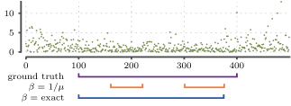
Figure 1: A toy data set $S$ with a burst between 100 and 400. Low values indicate short delays, bursts. The indicated regions are (i) the ground truth, (ii) bursts discovered with $\beta=1/\mu$, where $\mu$ is the average delay, and (iii) bursts discovered with $\beta$ set to the exact value of the generative model.

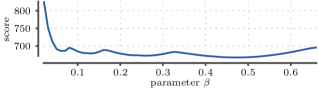
Figure 2: Score $\mathit{p_{exp}}\mathopen{}\left(S,L^{*};\alpha,\beta,k\right)$ as a function of $\beta$, where $\alpha=2$, $k=4$, and $L^{*}$ is the optimal level sequence for the given parameters. Low values are better.

Example 3.1.

Consider a sequence given in Figure 1, which shows a sequence of $500$ delays. The burst between 100 and 400 is generated using exponential model with $\lambda=1/2$, the remaining delays are generated using $\lambda=1$. We applied Viterbi with $\beta^{-1}$ equal to the average of the sequence, the value used by Kleinberg [13], and compare it to $\beta=1/2$, which is the correct ground level of the generative model. The remaining parameters were set to $\alpha=2$, $\gamma=1$, and $k=1$. We see that in the latter case we discover a burst that is much closer to the ground truth.∎

Our second remark is that if $\alpha$ and $\beta$ are given, one can easily discover the optimal bursts using Viterbi. The optimization becomes non-trivial when we need to optimize $\alpha$ and $\beta$ as well. To make matters worse, the score as a function of $\beta$ is non-convex, as demonstrated in Figure 2. Hence, we can easily get stuck in local minima.

Next, we introduce discrete variants of $\textsc{Exp}(\alpha)$ and Exp.

Problem 3.3 ($\textsc{Geo}(\alpha)$).

Given an integer delay sequence $S$, parameters $\alpha$, $\gamma$, and a maximum number of levels $k$, find a level sequence $L=\ell_{1},\ldots,\ell_{n}$, where $\ell_{i}$ is an integer $0\leq\ell_{i}\leq k$, and a parameter $\beta$, minimizing $\mathit{q_{geo}}\mathopen{}\left(L,S;\alpha,\beta,\gamma\right)$.

Problem 3.4 (Geo).

Given an integer delay sequence $S$, a parameter $\alpha$, and a maximum number of levels $k$, find a level sequence $L=\ell_{1},\ldots,\ell_{n}$, where $\ell_{i}$ is an integer $0\leq\ell_{i}\leq k$, and parameters $\alpha$ and $\beta$, minimizing $\mathit{q_{geo}}\mathopen{}\left(L,S;\alpha,\beta,\gamma\right)$.

Despite being very similar problems, we need to analyze these problems individually. We will show that $\textsc{Exp}(\alpha)$ can be solved exactly in polynomial time, although, the algorithm is too slow for practice. This approach does not work for other problems but we will show that all four problems can be $(1+\epsilon)$-approximated efficiently.

Before we continue, we need to address a pathological case when solving Exp: the problem of Exp is illdefined if the delay sequence $S$ contains a zero. To see this, assume that $s_{i}=0$. Then a level sequence $\ell_{i}=1$, and $\ell_{j}=0$, for $j\neq i$, with $\alpha=\infty$ and $\beta=1$ leads to a score of $-\infty$. This is because $\mathit{p_{exp}}\mathopen{}\left(s_{i};\beta\alpha\right)=\infty$ and the remaining terms are finite. This is why we assume that whenever we deal with Exp, we have $s_{i}>0$. If we have $s_{i}=0$, then we can either set $\alpha$ manually by using $\textsc{Exp}(\alpha)$ or shift the delays by a small amount.

4 Exact algorithm for $\textsc{Exp}(\alpha)$

In this section we present an exact polynomial algorithm for solving $\textsc{Exp}(\alpha)$. Unfortunately, this algorithm is impractically slow for large sequences: the time complexity is $\mathit{\mathcal{O}}\mathopen{}\left(n^{3}k^{4}\right)$ and the space complexity is $\mathit{\mathcal{O}}\mathopen{}\left(n^{3}k^{3}\right)$. Thus, it only serves as a theoretical result. More practical algorithms are given in the next sections.

In order to solve Exp we introduce a more complicated optimization problem.

Problem 4.1 (BndBurst).

Given a delay sequence $S=s_{1},\ldots,s_{n}$, a parameter $\alpha$, budget parameters $d$ and $m$, and a maximum number of levels $k$, find a level sequence $L=\ell_{1},\ldots,\ell_{n}$, with $0\leq l_{i}\leq k$, minimizing

$$\begin{split}&\sum_{i=1}^{n}\alpha^{l_{i}}s_{i}\quad\text{such that}\\ &\sum_{i}\max\left(\ell_{i}-\ell_{i-1},0\right)=d\quad\text{and}\quad\sum_{i}\ell_{i}=m\quad.\end{split}$$

We will show that this problem can be solved in polynomial time. But before, let us first show that Exp and BndBurst are intimately connected. See Appendix B for the proof.

Proposition 4.1.

Assume a delay sequence $S$, and parameters $\alpha$ and $\gamma$, and an upper bound for levels $k$. There are budget parameters $d\leq k(n+1)/2$ and $m\leq kn$ for which the level sequence $L$ solving BndBurst also solves $\textsc{Exp}(\alpha)$ along with

$$\beta=\frac{n}{\sum_{i}s_{i}\alpha^{\ell_{i}}}\quad.$$

We can solve BndBurst with a dynamic program. In order to do this, let us define a table $o$, where an entry $o[i,j,a,b]$ is the optimal score of the first $i$ symbols of the input sequence such that

$$\ell_{i}=j,\ \sum_{x=1}^{i}\max\left(\ell_{x}-\ell_{x-1},0\right)=a,\ \text{and}\ \sum_{x=1}^{i}\ell_{x}=b\quad.$$

In case, there is no level sequence satisfying the constraints, we set $o[i,j,a,b]=\infty$. Due to Proposition 4.1, we can limit $a\leq k(n+1)/2$ and $b\leq kn$. Consequently, $o$ contains $\mathit{\mathcal{O}}\mathopen{}\left(n^{3}k^{3}\right)$ entries. We can compute a single entry with

(4.1) $$\begin{split}&o[i,j,a,b]\\ &\quad=\alpha^{j}s_{i}+\min_{j^{\prime}}o[i-1,j^{\prime},a-\max(0,j-j^{\prime}),b-j]\quad.\end{split}$$

The computation of a single value thus requires $\mathit{\mathcal{O}}\mathopen{}\left(k\right)$ time. So computing the whole table can be done in $\mathit{\mathcal{O}}\mathopen{}\left(n^{3}k^{4}\right)$. Moreover, if we also store the optimal $j^{\prime}$ as given in Equation 4.1, for each cell, we can recover the level sequence responsible for every $o[i,j,a,b]$.

Proposition 4.1 now guarantees that we can solve Exp by comparing the level sequences responsible for $o[n,j,a,b]$, where $j=0,\ldots,k$, $a=0,\ldots,(k+1)n/2$, and $b=0,\ldots,kn$.

5 Approximating discrete burstiness

In this section we will provide a $(1+\epsilon)$-approximation algorithms for $\textsc{Geo}(\alpha)$ and Geo. The time complexities are stated in Table 1.

5.1 Approximating $\textsc{Geo}(\alpha)$

Note that if we knew the optimal $\beta$, then $\textsc{Geo}(\alpha)$ reduces to Problem 2.2, which we can solve in $\mathit{\mathcal{O}}\mathopen{}\left(nk\right)$ time by applying Viterbi. The idea behind our approximation is to test several values of $\beta$, and select the best solution among the tested values. The trick is to select values densely enough so that we can obtain $(1+\epsilon)$ guarantee while keeping the number of tests low, namely $\mathit{\mathcal{O}}\mathopen{}\left(\epsilon^{-1}\log\log n\right)$. The pseudo-code of the algorithm is given in Algorithm 1.

1 $\mu\leftarrow\frac{1}{n}\sum_{i}s_{i}$;

2 if $\mu=0$ then  return $L=\left(0,\ldots,0\right)$ ;

3 $\eta\leftarrow\mu/(\mu+1)$;

4 $c\leftarrow 1$;

5 while $\eta^{c}\leq\mu/(\mu+1/n)$ do

6       $\beta\leftarrow\eta^{c}$;

7       $L\leftarrow\textit{Viterbi}(S,\alpha,\beta,\gamma,k,\mathit{p_{geo}})$;

8       $c\leftarrow c/(1+\epsilon)$;

9      

10return the best observed $L$;

Algorithm 1 $\textit{GeoAlpha}(S,\alpha,\gamma,k,\epsilon)$

Next we state that the algorithm indeed yields an $(1+\epsilon)$-approximation ratio, and can be executed in $\mathit{\mathcal{O}}\mathopen{}\left(\epsilon^{-1}nk\log\log n\right)$ time. The proofs are given in Appendix C–D.

Proposition 5.1.

Let $S$ be an integer delay sequence, and let $\alpha$, $\gamma$, and $k$ be the parameters. Let $L^{*}$, $\beta^{*}$ be the solution to $\textsc{Geo}(\alpha)$. Assume $\epsilon>0$. Let $L$, $\beta$ be the solution returned by $\textit{GeoAlpha}(S,\alpha,\gamma,k,\epsilon)$. Then

$$\mathit{q_{geo}}\mathopen{}\left(S,L;\beta\right)\leq(1+\epsilon)\mathit{q_{geo}}\mathopen{}\left(S,L^{*};\beta^{*}\right)\quad.$$

Proposition 5.2.

The computational complexity of GeoAlpha is $\mathit{\mathcal{O}}\mathopen{}\left(\epsilon^{-1}nk\log\log n\right)$.

5.2 Approximating Geo

We now turn to approximating Geo. The approach here is similar to the previous approach: we test multiple values of $\alpha$ and invoke GeoAlpha. The pseudo-code for the algorithm is given in Algorithm 2.

1 $L\leftarrow\textit{GeoAlpha}(S,0,\gamma,k,\epsilon)$;

2 $\mu\leftarrow\frac{1}{n}\sum_{i}s_{i}$;

3 $\eta\leftarrow 1/(1+nk)$;

4 $\sigma\leftarrow\mu/(\mu+1/n)$;

5 $c\leftarrow 1$;

6 while $\eta^{c}\leq\sigma^{\epsilon/k}$ do

7       $\alpha\leftarrow\eta^{c}$;

8       $L\leftarrow\textit{GeoAlpha}(S,\alpha,\gamma,k,\epsilon)$;

9       $c\leftarrow c/(1+\epsilon)$;

10      

11return the best observed $L$;

Algorithm 2 $\textit{ApproxGeo}(S,\gamma,k,\epsilon)$

Next we establish the correctness of the method as well as the running time. The proofs are given in Appendix E–F.

Proposition 5.3.

Let $L^{*}$, $\alpha^{*}$, $\beta^{*}$ be the solution to Geo. Assume $\epsilon>0$. Let $L$, $\alpha$, $\beta$ be the solution returned by $\textit{ApproxGeo}(S,\gamma,k,\epsilon)$. Then

$$\mathit{q_{geo}}\mathopen{}\left(S,L;\alpha,\beta\right)\leq(1+\epsilon)\mathit{q_{geo}}\mathopen{}\left(S,L^{*};\alpha^{*},\beta^{*}\right)\quad.$$

Proposition 5.4.

The computational complexity of ApproxGeo is

$$\mathit{\mathcal{O}}\mathopen{}\left(nk\log\log n(\log n+\log\mu+\log k-\log\epsilon)\epsilon^{-2}\right)\quad.$$

6 Approximating continuous burstiness

In this section we will provide a $(1+\epsilon)$-approximation algorithms for $\textsc{Exp}(\alpha)$ and Exp. The time complexities are stated in Table 1.

6.1 Approximating $\textsc{Exp}(\alpha)$

In this section we introduce an approximation algorithm for $\textsc{Exp}(\alpha)$. The general approach of this algorithm is the same as in GeoAlpha: we test several values of $\beta$, solve the resulting subproblem with Viterbi, and select the best one. The pseudo-code is given in Algorithm 3.

1 $\mu\leftarrow\frac{1}{n}\sum_{i}s_{i}$;

2 $\beta\leftarrow 1/\mu$;

3 while $\beta\geq 1/(\alpha^{k}\mu)$ do

4       $L\leftarrow\textit{Viterbi}(S,\alpha,\beta,\gamma,k,\mathit{p_{exp}})$;

5       $\beta\leftarrow\beta/(1+\epsilon)$;

6      

7return the best observed $L$ and $\beta$;

Algorithm 3 $\textit{ExpAlpha}(S,\alpha,\gamma,k,\epsilon)$

Unlike with GeoAlpha, ExpAlpha does not yield an unconditional $(1+\epsilon)$-approximation guarantee. The key problem is that since exponential distribution is continuous, the term $\mathit{p_{exp}}\mathopen{}\left(s;\lambda\right)$ may be larger than $1$. Consequently, $-\log\mathit{p_{exp}}\mathopen{}\left(s;\lambda\right)$, as well as the actual score $\mathit{q_{exp}}$, can be negative. However, if the delay sequence has a geometric mean larger or equal than 1, we can guarantee the approximation ratio.

The proofs for the next two propositions are given in Appendix G–H.

Proposition 6.1.

Assume a delay sequence $S$, and parameters $\alpha$ and $\gamma$, and an upper bound for levels $k$. Let $\beta^{*}$ and $L^{*}$ be the solution to $\textsc{Exp}(\alpha(\alpha))$. Let $g=\left[\prod_{i}s_{i}\right]^{1/n}$ be the geometric mean. Assume $\epsilon>0$. Let $L$, $\beta$ be the solution returned by ExpAlpha. Then

$$\mathit{q_{exp}}\mathopen{}\left(S,L;\beta\right)-n\log g\leq(1+\epsilon)(\mathit{q_{exp}}\mathopen{}\left(S,L^{*};\beta^{*}\right)-n\log g)\quad.$$

Moreover, if $g\geq 1$, then

$$\mathit{q_{exp}}\mathopen{}\left(S,L;\beta\right)\leq(1+\epsilon)\mathit{q_{exp}}\mathopen{}\left(S,L^{*};\beta^{*}\right)\quad.$$

Note that if the geometric mean $g$ is less than 1, then we still have a guarantee, except now we need to shift the score by a (positive) constant of $-n\log g$.

Proposition 6.2.

The computational complexity of ExpAlpha is $\mathit{\mathcal{O}}\mathopen{}\left(\epsilon^{-1}nk^{2}\log\alpha\right)$.

6.2 Approximating Exp

We now turn to approximating Exp. The approach here is similar to the previous approach: we test multiple values of $\alpha$ and invoke ExpAlpha. The pseudo-code for the algorithm is given in Algorithm 4.

1 $\alpha\leftarrow(\max s_{i})/(\min s_{i})$;

2 $c\leftarrow\sqrt[2k]{1+\epsilon}$;

3 while $\alpha\geq 1$ do

4       $L\leftarrow\textit{ExpAlpha}(S,\alpha,\gamma,k,\epsilon/2)$;

5       $\alpha\leftarrow\alpha/c$;

6      

7return the best observed $L$;

Algorithm 4 $\textit{ApproxExp}(S,\gamma,k,\epsilon)$

Next we establish the correctness of the method as well as the running time. The proofs given in Appendix I–J.

Proposition 6.3.

Assume a delay sequence $S$, a parameter $\gamma$, and an upper bound for levels $k$. Let $\alpha^{*}$, $\beta^{*}$ and $L^{*}$ be the solution to Exp. Let $g=\left[\prod_{i}s_{i}\right]^{1/n}$ be the geometric mean, and let $\psi=n\log g$. Assume $\epsilon>0$. Let $L$, $\alpha$, $\beta$ the solution returned by ApproxExp. Then

$$\mathit{q_{exp}}\mathopen{}\left(S,L;\alpha,\beta\right)-\psi\leq(1+\epsilon)(\mathit{q_{exp}}\mathopen{}\left(S,L^{*};\alpha^{*},\beta^{*}\right)-\psi)\quad.$$

Moreover, if $g\geq 1$, then

$$\mathit{q_{exp}}\mathopen{}\left(S,L;\alpha,\beta\right)\leq(1+\epsilon)\mathit{q_{exp}}\mathopen{}\left(S,L^{*};\alpha,\beta^{*}\right)\quad.$$

Proposition 6.4.

Let $\Omega=\max s_{i}$ and let $\omega=\min s_{i}$. The computational complexity of ApproxExp is $\mathit{\mathcal{O}}\mathopen{}\left(\epsilon^{-2}nk^{3}\log^{2}(\Omega/\omega)\right)$.

6.3 Speeding up $\textsc{Exp}(\alpha)$

Our final step is to describe how can we speed-up the computation of $\textsc{Exp}(\alpha)$ in practice. The following proposition allows us to ignore a significant amount of tests.

Proposition 6.5.

Assume a delay sequence $S$, and parameters $\alpha$ and $\gamma$. Let $\beta$ be a parameter, and let $L$ be the optimal solution for $\textsc{Exp}(\alpha,\beta)$. Define

$$\beta^{\prime}=\frac{n}{\sum_{i}s_{i}\alpha^{\ell_{i}}}\quad.$$

Let $\beta^{*}$ be the optimal parameter to $\textsc{Exp}(\alpha)$. Then either

$$\beta^{*}\leq\min(\beta,\beta^{\prime})\quad\text{or}\quad\beta^{*}\geq\max(\beta,\beta^{\prime})\quad.$$

Proposition 6.5 allows us to ignore some tests: Let $\beta_{i}$ be the parameters tested by ExpAlpha, that is, $\beta_{i}=\mu^{-1}(1+\epsilon)^{-i}$. Assume that we test $\beta_{i}$, and compute $\beta^{\prime}$ as given in Proposition 6.5. If $\beta^{\prime}>\beta_{i}$, we can safely ignore testing any $\beta_{j}$ such that $\beta_{i}<\beta_{j}<\beta^{\prime}$. Similarly, if $\beta^{\prime}<\beta_{i}$, we can safely ignore testing any $\beta_{j}$ such that $\beta^{\prime}<\beta_{j}<\beta_{i}$.

The testing order of $\beta_{i}$ matters since we want to use both cases $\beta^{\prime}<\beta_{i}$ and $\beta^{\prime}>\beta_{i}$ efficiently. We propose the following order which worked well in our experimental evaluation: Let $t$ be the number of different $\beta_{i}$, and let $m$ be the largest integer for which $2^{m}\leq t$. Test the parameters in the order

$$0,2^{m},2^{m-1},2^{3(m-1)},\ldots,1,3,5,7,\ldots,$$

that is, we start with $0$ and increment by $2^{m}$ until we reach the end of the list. Then we decrease $m$ by 1, and repeat. During the traverse, we ignore the parameters that were already tested, as well as the redundant parameters.

Interestingly enough, this approach cannot be applied directly to the discrete version of the problem. First of all, the technique for proving Proposition 6.5 cannot be applied directly to the score function for the geometric distribution. Secondly, there is no closed formula for computing the discrete analogue of $\beta^{\prime}$ given in Proposition 6.5.

7 Related work

Discovering bursts Modelling and discovering bursts is a very well-studied topic in data mining. We will highlight some existing techniques. We are modelling delays between events, but we can alternatively model event counts in some predetermined window: high count indicate burst. Ihler et al. [11] proposed modelling such a statistic with Poisson process, while Fung et al. [5] used Binomial distribution. If the events at hand are documents, we can model burstiness with time-sensitive topic models [20, 14, 12]. As an alternative methods to discover bursts, Zhu and Shasha [21] used wavelet analysis, Vlachos et al. [19] applied Fourier analysis, and He and Parker [9] adopted concepts from Mechanics. Lappas et al. [16] propose discovering maximal bursts with large discrepancy.

Segmentation A sister problem of burstiness is a classic segmentation problem. Here instead of penalizing transitions, we limit the number of segments to $k$. If the overall score is additive w.r.t. the segments, then this problem can be solved in $\mathit{\mathcal{O}}\mathopen{}\left(n^{2}k\right)$ time [2]. For certain cases, this problem has a linear time solution [6]. Moreover, under some mild assumptions we can obtain a $(1+\epsilon)$ approximation in linear time [8].

Concept drift detection in data streams: A related problem setting to burstiness is concept drift detection. Here, a typical goal is to have an online algorithm that can perform update quickly and preferably does not use significant amount of memory. For an overview of existing techniques see an excellent survey by Gama et al. [7]. The algorithms introduced in this paper along with the original approach are not strictly online because in every case we need to know the mean of the sequence. However, if the mean is known, then we can run Viterbi in online fashion, and, if we are only interested in the burstiness of a current symbol, we need to maintain only $\mathit{\mathcal{O}}\mathopen{}\left(k\right)$ elements, per $\beta$.

8 Experimental evaluation

In this section we present our experiments. As a baseline we use method by Kleinberg [13], that is, we derive the parameter $\beta$ from $\mu$, the mean of the sequence. For exponential model, $\beta=\mu^{-1}$; we refer to this model as ExpMean. For geometrical model, $\beta=\mu/(\mu+1)$; we refer to this approach as GeoMean. Throughout the experiments, we used $\epsilon=0.05$ and $\gamma=1$ for our algorithms.

Experiments with synthetic data: We first focus on demonstrating when optimizing $\beta$ is more advantageous than the baseline approach.

For our first experiment we generated a sequence of $500$ data points. We planted a single burst with a varying length $50$–$250$. The burst was generated with $\mathit{p_{exp}}\mathopen{}\left(\cdot;1\right)$, while the remaining sequence was generated with $\mathit{p_{exp}}\mathopen{}\left(\cdot;2\right)$. We computed bursts with ExpMean and ExpAlpha, the parameters were set to $k=1$, $\alpha=2$. The obtained level sequence was evaluated by computing the hamming distance, $\sum_{i}{\left|\ell_{i}-\ell^{*}_{i}\right|}$, where $\ell^{*}_{i}$ is the ground truth level sequence. We repeated each experiment $100$ times.

We see from the results given in Figure 3 that the bursts discovered by ExpAlpha are closer to the ground truth, on average, than the baseline. This is especially the case when burst becomes larger. The main reason for this is that short bursts do not affect significantly the average of the sequence, $\mu$, so consequently, $\mu$ is close to the base activity level. As the burst increases, so does $\mu$, which leads to underestimating of $\beta$.

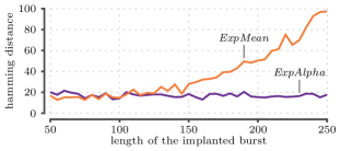
Figure 3: Hamming distance between the ground truth and the discovered level sequence as a function of the length of the planted burst. Low values are better.

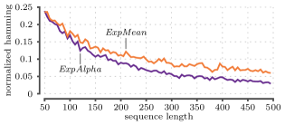
Figure 4: Hamming distance, normalized by the sequence length, between the ground truth level sequence and the discovered level sequence as a function of the sequence length. Low values are better.

Our next experiment is similar, expect now we vary the sequence length, $n$, (50–500) and set the burst length to be $n/3$. We generated the sequence as before, and we use the same parameters. In Figure 4 we report, $\frac{1}{n}\sum_{i}{\left|\ell_{i}-\ell^{*}_{i}\right|}$, the number of disagreements compared with the ground truth, normalized by $n$. Each experiment was repeated 300 times.

We see that for the shortest sequences, the number of disagreement is same for both algorithm, around $0.2$–$0.25$. This is due that we do not have enough samples to override the transition penalty $\mathit{\tau}$. Once the sequence becomes longer, we have more evidence of a burst, and here ExpAlpha starts to beat the baseline, due to a better model fit.

Experiments with real-world data: We considered two datasets: The first dataset, Crimes, consists of 17 033 crimes related to narcotics in Chicago between January and October, 2015. The second dataset, Mine, consists of 909 fatalities in U.S. mining industry dating from 2000, January.​ This data is visualized in Figure 6. In both datasets, each event has a time stamp: in Crimes we use minutes as granularity, whereas in Mine the time stamp is by the date. Using these time stamps, we created a delay sequence.

We applied ApproxExp, ExpAlpha, and ExpMean to Crimes. We set $k=4$, and for ExpAlpha and ExpMean we used $\alpha=2$. Since Crimes contains events with 0 delay, we added 1 minute to each delay to avoid the pathological case described in Section 3. The obtained bursts are presented in Figure 5. We also applied ApproxGeo, GeoAlpha, and GeoMean to Mine. Here we set $\alpha=1/2$ and $k=4$, however the algorithm used only 3 levels. The obtained bursts are presented in Figure 7.

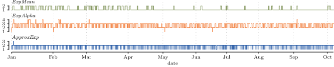
Figure 5: Discovered bursts in Crimes dataset.

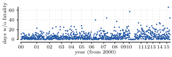
Figure 6: The delay sequence Mine, as well as the discovered bursts.

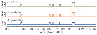
Figure 7: The delay sequence Mine, as well as the discovered bursts.

In Mine, the results by GeoAlpha and GeoMean are the same. However, we noticed that the results differ if we use different $\alpha$. The biggest difference between ApproxGeo and GeoAlpha is the last burst: GeoAlpha (and GeoMean) set the last burst to be on level 2, while ApproxGeo uses level 1. The reason for this is that ApproxGeo selects $\alpha$ to be very close to $0$, that is, much smaller than $1/2$, the parameter used by the other algoritms. This implies that when going one level up, the model expects the events to be much closer to each other.

In Crimes, ApproxExp and ExpAlpha discover burstier structure than ExpMean. ExpAlpha uses 4 different levels. Interestingly enough, in this level sequence, we spent most of the time at level 1, and we descended to level 0 for 3 short bursts. In other words, in addition to finding crime streaks, ExpAlpha also found three short periods when narcotics related crime rate was lower than usual. ApproxExp also spends most of its time on level 1 but often descends on level 0, while also highlighting one burst in early January.

Number of Viterbi calls: Next, we study relative efficiency when compared Viterbi. Since all 4 approximation schemes use Viterbi as a subroutine, a natural way of measuring the efficiency is to study the number of Viterbi calls. We report the number of calls as a function of $\epsilon$ for datasets Mine and Crimes in Figure 8. Here, we did not use the speed-up version of ExpAlpha.

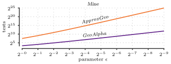
Figure 8: Number of Viterbi calls as a function of $\epsilon$. Both $x$ and $y$-axis are logarithmic. We set $k=4$, $\alpha=0.5$ for ExpAlpha, and $\alpha=2$ for ExpAlpha. Here, we did not use the speed-up version of ExpAlpha.

We see that the behaviour depends heavily on the accuracy parameter $\epsilon$: for example, if we use $\epsilon=0.5$, then GeoAlpha uses 17 calls while ApproxGeo uses 561 calls; if we set $\epsilon=2^{-9}$, then GeoAlpha needs 3453 calls while ApproxGeo needs 32 810 406 calls. This implies that we should not use extremely small $\epsilon$, especially if we also wish to optimize $\alpha$. Nevertheless, the algorithms are fast when we use moderately small $\epsilon$.

Effect of a speed-up: Finally, we compare the effect of a speed-up for ExpAlpha described in Section 6. Here we used both datasets Mine and Crimes to which we apply ExpAlpha with $k=5$ and $\alpha=2$. We vary $\epsilon$ from $2^{-13}$ to $1/2$ and compare the plain version vs. speed-up in Figure 9.

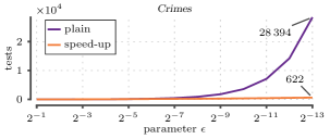
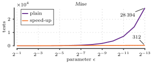
Figure 9: Number of tests needed as a function of $\epsilon$. Speed-up (see, Section 6) vs. vanilla version.

We see in Figure 9 that the we gain significant speed-up as we decrease $\epsilon$: At best, we improve by two orders of magnitude.

9 Concluding remarks

In this paper we presented variants of [13] for discovering bursts: instead of deriving the base rate from $\mu$, the average delay time between the events, we optimize this parameter along with the actual burst discovery. We showed that this leads to better burst discovery, especially if the bursts are long. We also propose variants, where we optimize the change parameter $\alpha$, instead of having it as a parameter.

Despite being a minor tweak, the resulting optimization problems are significantly harder. To solve the problems, we introduce efficient algorithms yielding $(1+\epsilon)$ approximation guarantee. These methods are based on testing multiple values for the base rate, and selecting the burst sequence with the best score. Despite being similar problems, discrete and continuous versions of the problem required their own algorithms. In addition, we were able significantly speed-up the exponential model variant by safely ignoring some candidate values for the base rate.

The approximation algorithms are quasi-linear with respect to sequence length. However, especially when we optimize $\alpha$, the algorithms depend also on the actual values of the sequence, see Table 1. A potential future work is to improve the algorithms, and develop polynomially strong approximation schemes. The other fruitful direction is to develop heuristics that allow us to ignore large parts of the parameters, similar to the speed-up we propose for the exponential model variant of the problem.

A Viterbi algorithm for solving Problem 2.1 or Problem 2.2

We can solve Problem 2.1 or Problem 2.2 using the standard dynamic programming algorithm by Viterbi [18]. Off-the-shelf version of this algorithm requires $\mathit{\mathcal{O}}\mathopen{}\left(nk^{2}\right)$ time. However, we can easily speed-up the algorithm to $\mathit{\mathcal{O}}\mathopen{}\left(nk\right)$.

To see this, let us first write $o[i,j]$ to express the optimal score for the $i$th first symbols such that the last level $\ell_{i}=j$. The Viterbi algorithm uses the fact that

$$o[i,j]=-\log p(s_{j},\beta\alpha^{j})+\min_{j^{\prime}}o[i-1,j^{\prime}]+\mathit{\tau}\mathopen{}\left(j^{\prime},j\right)$$

to solve the optimal sequence. Define two arrays

$$\begin{split}a[j]&=\min_{x\geq j}o[i-1,x]+\mathit{\tau}\mathopen{}\left(x,j\right)=\min_{j^{\prime}\geq j}o[i-1,x]\quad\text{and}\\ b[j]&=\min_{x\leq j}o[i-1,x]+\mathit{\tau}\mathopen{}\left(x,j\right)\quad.\end{split}$$

By definition, we have

$$o[i,j]=-\log p(s_{j},\beta\alpha^{j})+\min_{j^{\prime}\in\left\{a[j],b[j]\right\}}o[i-1,j^{\prime}]+\mathit{\tau}\mathopen{}\left(j^{\prime},j\right),$$

that is, we can compute $o[i,j]$ in constant time as long as we have $a[j]$ and $b[j]$. To compute $a[j]$ fast, note that either $a[j]=j$ or $a[j]=a[j+1]$, whichever produces better score. Similarly, due to linearity of $\mathit{\tau}$, we have $b[j]=j$ or $b[j]=b[j-1]$, whichever produces better score. This leads to a simple dynamic program given in Algorithm 5 that performs in $\mathit{\mathcal{O}}\mathopen{}\left(nk\right)$ time.

1 foreach $i=1,\ldots,n$ do

2       compute $a$ and $b$ in $\mathit{\mathcal{O}}\mathopen{}\left(k\right)$ time;

3       foreach $j=0,\ldots,k$ do

4             $c_{1}\leftarrow o[i-1,a[j]]$;

5             $c_{2}\leftarrow o[i-1,b[j]]+\mathit{\tau}\mathopen{}\left(b[j],j\right)$;

6             $o[i,j]\leftarrow\min(c_{1},c_{2})-\log p(s_{i};\beta\alpha^{j})$;

7            

8      

Algorithm 5 $\textit{Viterbi}(S,\alpha,\beta,\gamma,k,p)$, a dynamic program in order to discover burstiness

B Proof of Proposition 4.1

Proof.

Let $L$ and $\beta$ be the solution to $\textsc{Exp}(\alpha)$. Since

$$-\log\mathit{p_{exp}}\mathopen{}\left(s;\lambda\right)=s\lambda-\log\lambda,$$

we can decompose the score $\mathit{q_{exp}}\mathopen{}\left(L,S;\alpha,\beta,\gamma\right)$ as

$$\sum_{i=1}^{n}\beta\alpha^{\ell_{i}}s_{i}-\log\beta-\ell_{i}\log\alpha+\mathit{\tau}\mathopen{}\left(\ell_{i-1},\ell_{i}\right)\quad.$$

Define $d=\sum_{i}\max\left(\ell_{i}-\ell_{i-1},0\right)$ and $m=\sum_{i}\ell_{i}$. Let us also write $f(L)=\sum_{i}\alpha^{\ell_{i}}s_{i}$. Then the score becomes

(B.1) $$\beta f(L)-n\log\beta-m\log\alpha+d\gamma\log n\quad.$$

Obviously, $L$ satisfies the constraints posed in BndBurst. Moreover, $L$ minimizes $f(L)$ (within the constraints); otherwise we could replace $L$ with $L^{\prime}$, making the first term in Eq. B.1 genuinely smaller and keeping the remaining terms constant. This contradicts the optimality of $L$. Consequently, $L$ solves BndBurst.

To prove the remaining claims, first note that $\beta$ optimizing Eq. B.1 must satisfy

$$\frac{\partial\mathit{q_{exp}}}{\partial\beta}=f(L)-n/\beta=0,$$

proving the claim regarding $\beta$.

Since $\ell_{i}\leq k$, we have $m\leq nk$. To bound $d$, let us write $e=\sum_{i}\max\left(\ell_{i-1}-\ell_{i},0\right)$. We have

$$d-e=\sum_{i=1}^{n}\ell_{i}-\ell_{i-1}=\ell_{n}\leq k$$

and

$$d+e=\sum_{i=1}^{n}{\left|\ell_{i}-\ell_{i-1}\right|}\leq nk\quad.$$

Summing the inequalities leads to $2d\leq(n+1)k$, which proves the proposition. ∎

C Proof of Proposition 5.1

To prove the proposition we need several lemmas. Throughout this section, we assume that we are given an integer delay sequence $S$, and parameters $\alpha$, $\gamma$, $k$, and $\epsilon>0$. We will write $\mu=\frac{1}{n}\sum_{i}s_{i}$ and $c=1+\epsilon$.

The first lemma states that the optimal $\beta$ will be between the range that GeoAlpha tests.

Lemma C.1.

Let $L$ and $\beta$ be the solution of $\textsc{Geo}(\alpha)$. Then $\frac{\mu}{1+\mu}\leq\beta\leq\frac{\mu}{1/n+\mu}$.

Proof.

Since $\beta$ is optimal we must have $\partial\mathit{q_{geo}}\mathopen{}\left(S,L;\beta\right)/\partial\beta=0$. This implies that

$$\sum_{i=1}^{n}\frac{s_{i}}{\beta}=\sum_{i=1}^{n}\frac{1}{1-\beta\alpha^{\ell_{i}}}\quad\text{or}\quad\mu=\frac{1}{n}\sum_{i=1}^{n}\frac{\beta}{1-\beta\alpha^{\ell_{i}}}\quad.$$

Since $\alpha^{\ell_{i}}\leq 1$ we must have

$$\mu=\frac{1}{n}\sum_{i=1}^{n}\frac{\beta}{1-\beta\alpha^{\ell_{i}}}\leq\frac{\beta}{1-\beta},$$

which can be rewritten as $\mu/(1+\mu)\leq\beta$. This gives us the lower bound of the lemma.

To prove the other bound, note that we must have at least one $\ell_{i}=0$. This leads to

$$\mu=\frac{1}{n}\sum_{i=1}^{n}\frac{\beta}{1-\beta\alpha^{\ell_{i}}}\geq\frac{1}{n}\frac{\beta}{1-\beta},$$

which can be rewritten as $\mu/(n^{-1}+\mu)\geq\beta$. This proves the upper bound of the lemma. ∎

Next we show that if we vary $\alpha$ and $\beta$ by little, while keeping $L$ constant, the score will not change a lot.

Lemma C.2.

Let $\alpha^{\prime}$ such that $\alpha^{1+\epsilon}\leq\alpha^{\prime}\leq\alpha$ and let $\beta^{\prime}$ such that $\beta^{1+\epsilon}\leq\beta^{\prime}\leq\beta$. Then

$$\mathit{q_{geo}}\mathopen{}\left(L;\alpha^{\prime},\beta^{\prime}\right)\leq(1+\epsilon)\mathit{q_{geo}}\mathopen{}\left(L;\alpha,\beta\right)\quad.$$

Proof.

We can decompose the score $\mathit{q_{geo}}\mathopen{}\left(L;\alpha,\beta\right)$ as

$$\begin{split}&\sum_{i=1}^{n}-s_{i}\log\beta-s_{i}\ell_{i}\log\alpha-\log(1-\beta\alpha^{\ell_{i}})+\mathit{\tau}\mathopen{}\left(\ell_{i-1},\ell_{i}\right)\\ &\qquad=D\log\beta+E\log\alpha+C(\alpha,\beta),\\ \end{split}$$

where $C(\alpha,\beta)$ is the sum of the last two terms, $D=-\sum_{i=1}^{n}s_{i}$, and $E=-\sum_{i=1}^{n}\ell_{i}s_{i}$. Note that $C(\alpha,\beta)\geq 0$ and $C(\alpha,\beta)$ increases as a function of $\alpha$ and $\beta$. We can now upper bound the score

$$\begin{split}\mathit{q_{geo}}\mathopen{}\left(L;\alpha^{\prime},\beta^{\prime}\right)&=D\log\beta^{\prime}+E\log\alpha^{\prime}+C(\alpha^{\prime},\beta^{\prime})\\ &\leq D\log\beta^{c}+E\log\alpha^{c}+C(\alpha^{\prime},\beta^{\prime})\\ &=cD\log\beta+cE\log\alpha+C(\alpha^{\prime},\beta^{\prime})\\ &\leq cD\log\beta+cE\log\alpha+cC(\alpha,\beta)\\ &=c\mathit{q_{geo}}\mathopen{}\left(L;\alpha,\beta\right)\quad.\end{split}$$

Since $c=1+\epsilon$, this completes the proof. ∎

We can now prove the main result.

Proof of Prop. 5.1.

Lemma C.1 guarantees that GeoAlpha tests $\beta^{\prime}$ such that $(\beta^{*})^{1+\epsilon}\leq\beta^{\prime}\leq\beta^{*}$. Let $L^{\prime}$ be the optimal solution for $\beta^{\prime}$.

Lemma C.2 guarantees that $\mathit{q_{geo}}\mathopen{}\left(S,L^{*};\beta^{\prime}\right)\leq(1+\epsilon)\mathit{q_{geo}}\mathopen{}\left(S,L^{*};\beta^{*}\right)$. Since $\mathit{q_{geo}}\mathopen{}\left(S,L;\beta\right)\leq\mathit{q_{geo}}\mathopen{}\left(S,L^{\prime};\beta^{\prime}\right)\leq\mathit{q_{geo}}\mathopen{}\left(S,L^{*};\beta^{\prime}\right)$, the result follows. ∎

D Proof of Proposition 5.2

In order to prove the proposition we need two lemmas. The first lemma is a technical result that is needed to prove the second lemma.

Lemma D.1.

Define

$$h(x,y)=\log\log\frac{y+x}{x}\quad.$$

Then

$$h(x_{1},y_{2})-h(x_{1},y_{1})\geq h(x_{2},y_{2})-h(x_{2},y_{1})$$

for $x_{1}\leq x_{2}$ and $y_{1}\leq y_{2}$.

Proof.

The partial derivative of $h$ is equal to

$$\frac{\partial h(x,y)}{\partial x}=\left[\frac{1}{y+x}-\frac{1}{x}\right]\frac{1}{\log(y+x)-\log x},$$

and it is decreasing as a function of $y$. This implies that

$$\frac{\partial h(x,y_{2})}{\partial x}-\frac{\partial h(x,y_{1})}{\partial x}\leq 0,$$

that is $h(x,y_{2})-h(x,y_{1})$ is decreasing as a function of $x$, which proves the lemma. ∎

Our second lemma essentially shows that GeoAlpha does not test too many values.

Lemma D.2.

Let $n$ be an integer, and let $\mu\geq 1/n$ be a real number. Assume $\epsilon>0$ and let $c=1+\epsilon$. Let $r$ be such that

$$\beta^{(c^{r})}\geq\frac{\mu}{1+\mu},\quad{where}\quad\beta=\frac{\mu}{1/n+\mu}\quad.$$

Then

$$r\leq\frac{\log\log(n+1)-\log\log 2}{\log c}\in\mathit{\mathcal{O}}\mathopen{}\left(\frac{\log\log n}{\epsilon}\right)\quad.$$

Proof.

We begin by applying $-\log$ to the inequality $\beta^{(c^{r})}\geq\frac{\mu}{1+\mu}$ and obtain

$$c^{r}\log\frac{1/n+\mu}{\mu}\leq\log\frac{1+\mu}{\mu}\quad.$$

Another application of $\log$ and using $h$, as defined in Lemma D.1, leads us to

$$r\log c\leq h(\mu,1)-h(\mu,1/n)\quad.$$

Since $\mu\geq 1/n$, Lemma D.1 implies

$$\begin{split}r\log c&\leq h(\mu,1)-h(\mu,1/n)\\ &\leq h(1/n,1)-h(1/n,1/n)\\ &=\log\log\frac{1+1/n}{1/n}-\log\log\frac{2/n}{1/n}\\ &=\log\log(n+1)-\log\log 2,\\ \end{split}$$

which gives us the needed inequality. Since $1/\log c\leq\frac{1+\epsilon}{\epsilon}\in\mathit{\mathcal{O}}\mathopen{}\left(1/\epsilon\right)$, the result follows. ∎

We can now prove the main result.

Proof of Prop. 5.2.

Lemma D.2 guarantees that we only test $\mathit{\mathcal{O}}\mathopen{}\left(\epsilon^{-1}\log\log n\right)$ values of $\beta$. Each test requires $\mathit{\mathcal{O}}\mathopen{}\left(nk\right)$ time, which proves the result. ∎

E Proof of Proposition 5.3

Assume a delay sequence $S$, parameter $\gamma$, and an upper bound for levels $k$. Let $\alpha$, $\beta$ and $L$ be the solution to Geo. Let $\mu$ be the average of the $S$. Write $\Delta_{i}=\mathit{\tau}\mathopen{}\left(\ell_{i-1},\ell_{i}\right)$. Assume that we are given $\epsilon>0$ and let $c=1+\epsilon$.

First, we upper-bound the search space for $\alpha$.

Lemma E.1.

Let $\sigma=\frac{\mu}{1/n+\mu}$ and $\alpha^{\prime}=\sigma^{\epsilon/k}$. If $\alpha\geq\alpha^{\prime}$, then $\mathit{q_{geo}}\mathopen{}\left(L;\alpha^{\prime},\beta\right)\leq(1+\epsilon)\mathit{q_{geo}}\mathopen{}\left(L;\alpha,\beta\right)$

Proof.

Decompose the score $\mathit{q_{geo}}\mathopen{}\left(L\right)$ to

$$\sum_{i=1}^{n}-s_{i}\log\beta-s_{i}\ell_{i}\log\alpha-\log(1-\beta\alpha^{\ell_{i}})+\Delta_{i}\quad.$$

Let $C(\alpha)$ be the sum of the last two terms. Since $C(\alpha)\geq C(\alpha^{\prime})\geq 0$, we only need to show that

$$-s_{i}\log\beta-s_{i}\ell_{i}\log\alpha^{\prime}\leq-cs_{i}\log\beta-cs_{i}\ell_{i}\log\alpha\quad.$$

To show this, note that Lemma C.1 implies that $\beta\leq\sigma$. We can now bound the first two terms by

$$\begin{split}-s_{i}\log\beta-s_{i}\ell_{i}\log\alpha^{\prime}&=-s_{i}\log\beta-\epsilon s_{i}\frac{\ell_{i}}{k}\log\sigma\\ &\leq-s_{i}\log\beta-\epsilon s_{i}\frac{\ell_{i}}{k}\log\beta\\ &\leq-s_{i}\log\beta-\epsilon s_{i}\log\beta\\ &=-cs_{i}\log\beta\\ &\leq-cs_{i}\log\beta-cs_{i}\ell_{i}\log\alpha\quad.\\ \end{split}$$

This proves the lemma. ∎

Next, we lower-bound the search space for $\alpha$.

Lemma E.2.

If there is an index $j$ such that $s_{j}l_{j}\neq 0$, then $\alpha\geq\frac{1}{1+nk}$.

Proof.

In order for $\alpha$ to be optimal, $\frac{\partial\mathit{q_{geo}}}{\partial\alpha}=0$, or

$$\sum_{i=1}^{n}s_{i}\ell_{i}=\sum_{i=1}^{n}\frac{\beta\ell_{i}\alpha^{\ell_{i}}}{1-\beta\alpha^{\ell_{i}}}=\sum_{i=1}^{n}f(\alpha,\beta,l_{i}),$$

We can upper bound the right-hand side. If $\ell_{i}=0$, then

$$\frac{\beta\ell_{i}\alpha^{\ell_{i}}}{1-\beta\alpha^{\ell_{i}}}=0\leq\frac{k\alpha}{1-\alpha}\quad.$$

If $\ell_{i}\geq 1$, then

$$\frac{\beta\ell_{i}\alpha^{\ell_{i}}}{1-\beta\alpha^{\ell_{i}}}\leq\ell_{i}\frac{\beta\alpha}{1-\beta\alpha}\leq k\frac{\beta\alpha}{1-\beta\alpha}\leq k\frac{\alpha}{1-\alpha}\quad.$$

This leads to

$$\sum_{i=1}^{n}s_{i}\ell_{i}\leq kn\frac{\alpha}{1-\alpha}.$$

Since $s_{j}l_{j}\geq 1$, we have

$$\frac{\alpha}{1-\alpha}\geq\frac{1}{nk}\sum_{i=1}^{n}s_{i}\ell_{i}\geq\frac{1}{nk},$$

which can be rewritten as $\alpha\geq\frac{1}{1+nk}$. ∎

The next lemma addressed the case when the condition of the previous lemma fails.

Lemma E.3.

If $s_{i}l_{i}=0$ for all $i$, then $\alpha=0$.

Proof.

We can decompose the score $\mathit{q_{geo}}\mathopen{}\left(L\right)$ as

$$\sum_{i=1}^{n}-s_{i}\log\beta-\log(1-\beta\alpha^{\ell_{i}})+\Delta_{i}\quad.$$

This score decreases as a function of $\alpha$, and is minimized when $\alpha=0$. ∎

We can now prove the main result.

Proof of Prop. 5.3.

If the condition in Lemma E.3 is triggered, then $\alpha=0$, which is tested by ApproxGeo, and Proposition 5.1 guarantees the result.

Otherwise, Lemmas C.1, E.1 and E.2 guarantee that ApproxGeo tests $\alpha^{\prime}$ and $\beta^{\prime}$ such that $(\beta^{*})^{1+\epsilon}\leq\beta^{\prime}\leq\beta^{*}$ and $(\alpha^{*})^{1+\epsilon}\leq\alpha^{\prime}\leq\alpha^{*}$. Let $L^{\prime}$ be the optimal solution for $\alpha^{\prime}$, $\beta^{\prime}$.

The proposition follows since

$$\mathit{q_{geo}}\mathopen{}\left(L^{\prime};\alpha^{\prime},\beta^{\prime}\right)\leq\mathit{q_{geo}}\mathopen{}\left(L^{*};\alpha^{\prime},\beta^{\prime}\right)\leq c\mathit{q_{geo}}\mathopen{}\left(L^{*};\alpha^{*},\beta^{*}\right),$$

where the second inequality is due to Lemma C.2. ∎

F Proof of Proposition 5.4

Proof.

Let $\sigma=\mu/(1/n+\mu)$. Let $m$ be the number of tests for different $\alpha$s. The stopping condition now guarantees

$$\left(\frac{1}{1+nk}\right)^{c^{-m}}\leq\sigma^{\epsilon/k},$$

which can be rewritten as

$$-c^{-m}\log(1+nk)\leq\frac{\epsilon}{k}\log\sigma\leq\frac{\epsilon}{k}(\sigma-1)=\frac{-\epsilon}{k(1+n\mu)}$$

Reversing the sign, and taking logarithm leads to

$$-m\log c\geq\log(\epsilon)-\log(k)-\log(1+n\mu)-\log\log(1+nk)$$

which leads to

$$\begin{split}m&\leq\frac{\log(k)+\log(1+n\mu)-\log(\epsilon)+\log\log(1+nk)}{\log c}\\ &\in\mathit{\mathcal{O}}\mathopen{}\left(\frac{\log n+\log\mu+\log k-\log\epsilon}{\epsilon}\right)\quad.\end{split}$$

∎

G Proof of Proposition 6.1

To prove the proposition we need several lemmas. Throughout this section, we assume that we are given a delay sequence $S$, and parameters $\alpha$, $\gamma$ and $k$. We will write $\mu=\frac{1}{n}\sum_{i}s_{i}$.

First, we need to show that the optimal $\beta$ stays within the bounds used by ApproxExp.

Lemma G.1.

Let $\beta$ and $L$ be the solution to $\textsc{Exp}(\alpha)$. Then $\frac{1}{\alpha^{k}\mu}\leq\beta\leq\frac{1}{\mu}$.

Proof.

Write $\Delta_{i}=\mathit{\tau}\mathopen{}\left(\ell_{i-1},\ell_{i}\right)$. We can decompose the score $\mathit{q_{exp}}\mathopen{}\left(L;\beta\right)$ as

$$\sum_{i=1}^{n}\beta\alpha^{\ell_{i}}s_{i}-\log\beta-\ell_{i}\log\alpha+\Delta_{i}\quad.$$

Let $g=\frac{1}{n}\sum_{i}\alpha^{\ell_{i}}s_{i}$. Due to optimality of $\beta$ we must have

$$\frac{\partial\mathit{q_{exp}}}{\partial\beta}=ng-\frac{n}{\beta}=0,$$

that is, $\beta=1/g$. As $0\leq\ell_{i}\leq k$, we have $\mu\leq g\leq\alpha^{k}\mu$. This proves the lemma. ∎

Our next result is a technical lemma that is needed to control the possible negative terms in the score.

Lemma G.2.

Let $\beta$ and $L$ be the solution to Exp. Let $g=\left[\prod_{i}s_{i}\right]^{1/n}$ be the geometric mean. Then

$$\sum_{i=1}^{n}-\log\beta-\ell_{i}\log\alpha\geq n\log g\quad.$$

Proof.

Let $f=\frac{1}{n}\sum_{i}\alpha^{\ell_{i}}s_{i}$ and $h=\left[\prod_{i}\alpha^{\ell_{i}}\right]^{1/n}$. The arithmetic-geometric mean inequality states that $hg\leq f$. By definition, we must have $\beta=1/f$. This leads to

$$\begin{split}\sum_{i=1}^{n}-\log\beta-\ell_{i}\log\alpha&=n\log f-\sum_{i=1}^{n}\ell_{i}\log\alpha\\ &\geq n\log gh-\sum_{i=1}^{n}\ell_{i}\log\alpha\\ &=n\log g+n\log h-\sum_{i=1}^{n}\ell_{i}\log\alpha\\ &=n\log g\quad.\\ \end{split}$$

This proves the lemma. ∎

The next lemma shows that if we vary $\beta$ by little while keeping $L$ constant, the score of the solution will not change a lot.

Lemma G.3.

Let $\beta$ and $L$ be the solution to Exp. Let $g=\left[\prod_{i}s_{i}\right]^{1/n}$ be the geometric mean, and let $\psi=n\log g$. Let $\epsilon_{1},\epsilon_{2}>0$ and assume $\alpha^{\prime}$, $\beta^{\prime}$ such that $\beta\leq\beta^{\prime}\leq\beta(1+\epsilon_{1})$ and $\alpha\leq\alpha^{\prime}\leq\alpha(1+\epsilon_{2})$. Then

$$\mathit{q_{exp}}\mathopen{}\left(L;\alpha^{\prime},\beta^{\prime}\right)-\psi\leq c(\mathit{q_{exp}}\mathopen{}\left(L;\alpha,\beta\right)-\psi),$$

where $c=(1+\epsilon_{1})(1+\epsilon_{2})^{k}$.

Proof.

Write $\Delta_{i}=\mathit{\tau}\mathopen{}\left(\ell_{i-1},\ell_{i}\right)$. Decompose the score $\mathit{q_{exp}}\mathopen{}\left(L;\alpha,\beta\right)$ to

$$\sum_{i=1}^{n}\beta\alpha^{\ell_{i}}s_{i}-\log\beta-\ell_{i}\log\alpha+\Delta_{i},$$

and let $C(\alpha,\beta)$ be the sum of last three terms. Note that $C(\alpha^{\prime},\beta^{\prime})\leq C(\alpha,\beta)$, and due to Lemma G.2 $C(\alpha,\beta)\geq\psi$. Also let $F(\alpha)=\sum_{i=1}^{n}\alpha^{\ell_{i}}s_{i}$ be the sum of the first term without $\beta$. We can now write

$$\begin{split}\mathit{q_{exp}}\mathopen{}\left(L;\alpha^{\prime},\beta^{\prime}\right)-\psi&=\beta^{\prime}F(\alpha^{\prime})+C(\alpha^{\prime},\beta^{\prime})-\psi\\ &\leq c\beta F(\alpha)+C(\alpha,\beta)-\psi\\ &\leq c\beta F(\alpha)+c(C(\alpha,\beta)-\psi)\\ &=c(\mathit{q_{exp}}\mathopen{}\left(L;\alpha,\beta\right)-\psi),\\ \end{split}$$

which proves the lemma. ∎

We can now prove the main result.

Proof of Prop. 6.1.

Lemma G.1 guarantees that ApproxExp tests $\beta^{\prime}$ such that $\beta^{*}\leq\beta^{\prime}\leq\beta^{*}(1+\epsilon)$. Let $L^{\prime}$ be the optimal solution for $\beta^{\prime}$.

Lemma G.3 guarantees that $\mathit{q_{exp}}\mathopen{}\left(L^{*};\beta^{\prime}\right)-n\log g\leq(1+\epsilon)(\mathit{q_{exp}}\mathopen{}\left(L^{*};\beta^{*}\right)-n\log g)$. Since $\mathit{q_{exp}}\mathopen{}\left(L;\beta\right)\leq\mathit{q_{exp}}\mathopen{}\left(L^{\prime};\beta^{\prime}\right)\leq\mathit{q_{exp}}\mathopen{}\left(L^{*};\beta^{\prime}\right)$, the result follows. ∎

H Proof of Proposition 6.2

Proof.

Assume that $(1+\epsilon)^{-r}/\mu\geq 1/(\alpha^{k}\mu)$. Solving for $r$ gives us

$$r\leq\frac{k\log\alpha}{\log(1+\epsilon)}\in\mathit{\mathcal{O}}\mathopen{}\left(\epsilon^{-1}k\log\alpha\right)\quad.$$

Consequently, ApproxExp has at most $\mathit{\mathcal{O}}\mathopen{}\left(\epsilon^{-1}k\log\alpha\right)$ iterations. Since a single iteration costs $\mathit{\mathcal{O}}\mathopen{}\left(nk\right)$ time, the result follows. ∎

I Proof of Proposition 6.3

We first upper-bound the optimal $\alpha$.

Lemma I.1.

Let $\Omega=\max S$ and $\omega=\min S$. Then $\alpha\leq\Omega/\omega$.

Proof.

Assume that $\alpha>\Omega/\omega$. To prove the result we use the fact that

(I.2) $$s_{i}\lambda^{\prime}-\log\lambda^{\prime}\leq s_{i}\lambda-\log\lambda,$$

when $s_{i}\geq\lambda^{\prime}\geq\lambda$ or $s_{i}\leq\lambda^{\prime}\leq\lambda$.

We claim that $\beta\alpha\geq\omega$. Assume otherwise. Consider an alternative level sequence $\ell^{\prime}_{i}=\max(\ell_{i}-1,0)$ and $\beta^{\prime}=\beta\alpha$. Under this transformation, the only modelling terms in $\mathit{p_{exp}}$ that change are the original levels for which $\ell_{i}=0$, equal to

$$(\beta^{\prime}s_{i}-\log\beta^{\prime})-(\beta s_{i}-\log\beta)\quad.$$

Eq. I.2 guarantees that this change is always negative. In addition, $\Delta_{i}$ can only decrease. We can repeat this argument until $\beta\alpha\geq\omega$.

We now split in two separate cases.

Case (i): Assume $\beta\alpha\geq\Omega$. We must have $\beta\alpha=\Omega$. Otherwise, since $\beta\alpha>s_{i}$, Eq. I.2 now guarantees that we can safely decrease $\alpha$ at least until $\beta\alpha=\Omega$. The assumption $\alpha>\Omega/\omega$ implies that $\beta\leq\omega$. Similarly, we must have $\beta=\omega$. Otherwise, if we increase $\beta$ and decrease $\alpha$ such that $\beta\alpha$ remains constant, then Eq. I.2 implies that the score decreases until $\beta=\omega$. Consequently, $\alpha=\Omega/\omega$ which contradicts the assumption $\alpha>\Omega/\omega$.

Case (ii): Assume $\beta\alpha\leq\Omega$. In other words we have $\beta\leq\omega\leq\beta\alpha\leq\Omega\leq\beta\alpha^{2}$. We claim that $\beta=\omega$ or $\Omega=\beta\alpha^{2}$. Otherwise, increase $\beta$ and decrease $\alpha$ such that $\beta\alpha$ remains constant; Eq. I.2 states that we can only decrease the score at least until $\beta=\omega$ or $\Omega=\beta\alpha^{2}$. This immediately implies $\alpha\leq\Omega/\omega$, which is a contradiction. ∎

Proof of Prop. 6.3.

Lemma I.1 guarantees that ApproxExp tests $\alpha^{\prime}$ such that $\alpha\leq\alpha^{\prime}\leq\alpha\sqrt[2k]{1+\epsilon}$. Lemma G.3 now guarantees the approximation ratio of

$$(1+\epsilon/2)\sqrt[2k]{1+\epsilon}^{k}\leq(1+\epsilon),$$

which proves the result. ∎

J Proof of Proposition 6.4

Proof.

The number of iterations done by ApproxExp is $\mathit{\mathcal{O}}\mathopen{}\left(\epsilon^{-1}k(\log\Omega-\log\omega)\right)$. A single iteration requires $\mathit{\mathcal{O}}\mathopen{}\left(\epsilon^{-1}nk^{2}\log\alpha\right)\in\mathit{\mathcal{O}}\mathopen{}\left(\epsilon^{-1}nk^{2}\log(\Omega/\omega)\right)$ time. ∎

K Proof of Proposition 6.5

Let us write $\lambda(\beta)$ to be an optimal solution using $\beta$ as a parameter. Define

$$f(L)=\sum_{i=1}^{n}s_{i}\alpha^{\ell_{i}},$$

and let $h(\beta)=n/f(\lambda(\beta))$. Note that we may have several optimal solutions for $\lambda(\beta)$ and they may yield different values of $f(L)$. We break the ties with a lexicographical order.

We will first prove that $h$ is monotonic.

Lemma K.1.

$h(\beta_{1})\geq h(\beta_{2})$ for $\beta_{1}\leq\beta_{2}$.

Proof.

Similar to Eq. B.1, we can decompose the score $\mathit{q_{exp}}\mathopen{}\left(L,S;\alpha,\beta,\gamma\right)=\beta f(L)-n\log\beta+C(L)$, where

$$C(L)=\sum_{i=1}^{n}-\ell_{i}\log\alpha+\mathit{\tau}\mathopen{}\left(\ell_{i-1},\ell_{i}\right)\quad.$$

We will suppress $S$, $\alpha$, and $\gamma$ from the notation since they are constant.

Assume that we have two level sequences $L_{1}$ and $L_{2}$. Note that if

$$\beta f(L_{1})-n\log\beta+C(L_{1})=\beta f(L_{2})-n\log\beta+C(L_{2})$$

then

$$\beta f(L_{1})+C(L_{1})=\beta f(L_{2})+C(L_{2})\quad.$$

This implies that there are three possible cases: (i) $L_{1}$ and $L_{2}$ yield exact same cost for every $\beta$, (ii) the cost for $L_{1}$ is always smaller than the cost for $L_{2}$, or vice versa, or (iii) there is exactly one parameter, say $\beta^{\prime}$, where $\mathit{q_{exp}}\mathopen{}\left(L_{1};\beta^{\prime}\right)=\mathit{q_{exp}}\mathopen{}\left(L_{2};\beta^{\prime}\right)$. In the first case, we must have $f(L_{1})=f(L_{2})$. In the last case, we must have $f(L_{1})\neq f(L_{2})$. Assume that $f(L_{1})<f(L_{2})$. Then for every $\beta\leq\beta^{\prime}$,

$$\begin{split}&\mathit{q_{exp}}\mathopen{}\left(L_{1};\beta\right)-\mathit{q_{exp}}\mathopen{}\left(L_{2};\beta\right)\\ &=\beta(f(L_{1})-f(L_{2}))+C(L_{1})-C(L_{2})\\ &\geq\beta^{\prime}(f(L_{1})-f(L_{2}))+C(L_{1})-C(L_{2})\\ &=\mathit{q_{exp}}\mathopen{}\left(L_{1};\beta^{\prime}\right)-\mathit{q_{exp}}\mathopen{}\left(L_{2};\beta^{\prime}\right)=0,\\ \end{split}$$

and similarly $\mathit{q_{exp}}\mathopen{}\left(L_{1};\beta\right)\leq\mathit{q_{exp}}\mathopen{}\left(L_{2};\beta\right)$, for every $\beta\geq\beta^{\prime}$.

Let $\beta_{1}<\beta_{2}$, and let $L_{1}=\lambda(\beta_{1})$ and $L_{2}=\lambda(\beta_{2})$. There are four possible cases.

Case (a): If $\mathit{q_{exp}}\mathopen{}\left(L_{1};\beta_{1}\right)=\mathit{q_{exp}}\mathopen{}\left(L_{2};\beta_{1}\right)$ and $\mathit{q_{exp}}\mathopen{}\left(L_{1};\beta_{2}\right)=\mathit{q_{exp}}\mathopen{}\left(L_{2};\beta_{2}\right)$, then Case (i) guarantees that $f(L_{1})=f(L_{2})$.

Case (b): If $\mathit{q_{exp}}\mathopen{}\left(L_{1};\beta_{1}\right)=\mathit{q_{exp}}\mathopen{}\left(L_{2};\beta_{1}\right)$ and $\mathit{q_{exp}}\mathopen{}\left(L_{1};\beta_{2}\right)>\mathit{q_{exp}}\mathopen{}\left(L_{2};\beta_{2}\right)$, then Case (iii) guarantees that $\beta_{1}=\beta^{\prime}$ and $f(L_{1})\geq f(L_{2})$.

Case (c): If $\mathit{q_{exp}}\mathopen{}\left(L_{1};\beta_{1}\right)<\mathit{q_{exp}}\mathopen{}\left(L_{2};\beta_{1}\right)$ and $\mathit{q_{exp}}\mathopen{}\left(L_{1};\beta_{2}\right)=\mathit{q_{exp}}\mathopen{}\left(L_{2};\beta_{2}\right)$, then Case (iii) guarantees that $\beta_{2}=\beta^{\prime}$ and $f(L_{1})\geq f(L_{2})$.

Case (d): If $\mathit{q_{exp}}\mathopen{}\left(L_{1};\beta_{1}\right)<\mathit{q_{exp}}\mathopen{}\left(L_{2};\beta_{1}\right)$ and $\mathit{q_{exp}}\mathopen{}\left(L_{1};\beta_{2}\right)>\mathit{q_{exp}}\mathopen{}\left(L_{2};\beta_{2}\right)$, then Case (iii) guarantees that $\beta_{1}<\beta^{\prime}<\beta_{2}$ and $f(L_{1})\geq f(L_{2})$.

These cases immediately guarantee that $h(\beta_{1})=n/f(L_{1})\leq n/f(L_{2})=h(\beta_{2}).$ ∎

Proof of Proposition 6.5.

Since $\beta^{*}$ is optimal we must have $\beta^{*}=h(\beta^{*})$. Assume that $\beta\leq\beta^{*}$. Then Lemma K.1 states that $\beta^{\prime}=h(\beta)\leq h(\beta^{*})=\beta^{*}$. Assume that $\beta^{*}\leq\beta$. Then Lemma K.1 states that $\beta^{*}=h(\beta^{*})\leq h(\beta)=\beta^{\prime}$. ∎

References

• Backstrom et al. [2006] L. Backstrom, D. Huttenlocher, J. Kleinberg, and X. Lan. Group formation in large social networks: Membership, growth, and evolution. In KDD, pages 44–54, 2006.
• Bellman [1961] R. Bellman. On the approximation of curves by line segments using dynamic programming. Communications of the ACM, 4(6), 1961.
• Chen [2006] C. Chen. Citespace II: Detecting and visualizing emerging trends and transient patterns in scientific literature. J. Am. Soc. Inf. Sci. Technol., 57(3):359–377, 2006.
• Fontugne et al. [2011] R. Fontugne, K. Cho, Y. Won, and K. Fukuda. Disasters seen through flickr cameras. In SWID, 2011.
• Fung et al. [2005] G. P. C. Fung, J. X. Yu, P. S. Yu, and H. Lu. Parameter free bursty events detection in text streams. In VLDB, pages 181–192, 2005.
• Galil and Park [1990] Z. Galil and K. Park. A linear-time algorithm for concave one-dimensional dynamic programming. Inf. Process. Lett., 33(6):309–311, 1990.
• Gama et al. [2014] J. Gama, I. Zliobaite, A. Bifet, M. Pechenizkiy, and A. Bouchachia. A survey on concept drift adaptation. ACM Comput. Surv., 46(4):44:1–44:37, 2014.
• Guha et al. [2006] S. Guha, N. Koudas, and K. Shim. Approximation and streaming algorithms for histogram construction problems. TODS, 31(1):396–438, 2006.
• He and Parker [2010] D. He and D. S. Parker. Topic dynamics: An alternative model of bursts in streams of topics. In KDD, 2010.
• He et al. [2011] Q. He, D. Kifer, J. Pei, P. Mitra, and C. L. Giles. Citation recommendation without author supervision. In WSDM, pages 755–764, 2011.
• Ihler et al. [2006] A. Ihler, J. Hutchins, and P. Smyth. Adaptive event detection with time-varying poisson processes. In KDD, pages 207–216, 2006.
• Kawamae [2011] N. Kawamae. Trend analysis model: Trend consists of temporal words, topics, and timestamps. In WSDM, pages 317–326, 2011.
• Kleinberg [2003] J. Kleinberg. Bursty and hierarchical structure in streams. DMKD, 7(4):373–397, 2003.
• Krause et al. [2006] A. Krause, J. Leskovec, and C. Guestrin. Data association for topic intensity tracking. In ICML, pages 497–504, 2006.
• Kumar et al. [2003] R. Kumar, J. Novak, P. Raghavan, and A. Tomkins. On the bursty evolution of blogspace. In WWW, pages 568–576, 2003.
• Lappas et al. [2009] T. Lappas, B. Arai, M. Platakis, D. Kotsakos, and D. Gunopulos. On burstiness-aware search for document sequences. In KDD, pages 477–486, 2009.
• Mane and Börner [2004] K. K. Mane and K. Börner. Mapping topics and topic bursts in PNAS. PNAS, 101(suppl 1):5287–5290, 2004.
• Viterbi [1967] A. Viterbi. Error bounds for convolutional codes and an asymptotically optimum decoding algorithm. IEEE IT, 13(2):260–269, 1967.
• Vlachos et al. [2004] M. Vlachos, C. Meek, Z. Vagena, and D. Gunopulos. Identifying similarities, periodicities and bursts for online search queries. In SIGMOD, pages 131–142, 2004.
• Wang and McCallum [2006] X. Wang and A. McCallum. Topics over time: A non-markov continuous-time model of topical trends. In KDD, pages 424–433, 2006.
• Zhu and Shasha [2003] Y. Zhu and D. Shasha. Efficient elastic burst detection in data streams. In KDD, pages 336–345, 2003.