Abstract

$SO(5)\times U(1)\times SU(3)$ gauge-Higgs unification model inspired by $SO(11)$ gauge-Higgs grand unification is constructed in the Randall-Sundrum warped space. The 4D Higgs boson is identified with the Aharonov-Bohm phase in the fifth dimension. Fermion multiplets are introduced in the bulk in the spinor, vector and singlet representations of $SO(5)$ such that they are implemented in the spinor and vector representations of $SO(11)$. The mass spectrum of quarks and leptons in three generations is reproduced except for the down quark mass. The small neutrino masses are explained by the gauge-Higgs seesaw mechanism which takes the same form as in the inverse seesaw mechanism in grand unified theories in four dimensions.

1 Introduction

The existence of the Higgs boson of a mass 125 GeV has been firmly established at LHC.[1] It supports the unification scenario of electromagnetic and weak forces. So far almost all of the experimental results and observations have been consistent with the standard model (SM) based on the gauge group ${\cal G}_{\rm SM}=SU(3)_{C}\times SU(2)_{L}\times U(1)_{Y}$. Yet it is not clear whether or not the observed Higgs boson is precisely what the SM assumes. All of the Higgs couplings to other fields and to itself need to be determined with better accuracy. Furthermore, the SM is afflicted with the gauge hierarchy problem which becomes apparent when the model is generalized to incorporate grand unification. The fundamental problem is the lack of a principle which regulates the Higgs sector, in quite contrast to the gauge sector which is controlled by the gauge principle.

There are several attempts to overcome these difficulties. Supersymmetric theory is one of them which has been extensively investigated. An alternative approach is gauge-Higgs unification in which the Higgs boson is identified with the zero mode of the fifth dimensional component of the gauge potential. It appears as a fluctuation mode of the Aharonov-Bohm (AB) phase $\theta_{H}$ in the fifth dimension.[2]-[7] Already a realistic gauge-Higgs unification (GHU) model has been constructed. It is the $SO(5)\times U(1)_{X}$ gauge theory in the Randall-Sundrum (RS) warped space with quark and lepton multiplets in the vector representation of $SO(5)$.[8]-[16] It has been shown that the $SO(5)\times U(1)_{X}$ GHU yields nearly the same phenomenology at low energies as the SM. Deviations of the gauge couplings of quarks and leptons from the SM values are less than $10^{-3}$ for $\theta_{H}\sim 0.1$. Higgs couplings of quarks, leptons, $W$ and $Z$ are approximately the SM values times $\cos\theta_{H}$, the deviation being about 1%. The Kaluza-Klein (KK) mass scale is about $m_{\rm KK}\sim 8\,$TeV for $\theta_{H}\sim 0.1$. Implications of GHU to dark matter and Majorana neutrino masses are also under intensive study.[17]-[21]

The model predicts $Z^{\prime}$ bosons, which are the first KK modes of $\gamma$, $Z$, and $Z_{R}$ ($SU(2)_{R}$ gauge boson), in the $7\sim 9\,$TeV range for $\theta_{H}=0.1\sim 0.07$. They have broad widths and can be produced at 14 TeV LHC.[12, 13] The current non-observation of $Z^{\prime}$ signals puts the limit $\theta_{H}<0.11$. Right-handed quarks and charged leptons have rather large couplings to $Z^{\prime}$. It has been pointed out recently that the interference effects of $Z^{\prime}$ bosons can be clearly observed at 250 GeV $e^{+}e^{-}$ linear collider (ILC).[14, 16] For instance, in the process $e^{+}e^{-}\rightarrow\mu^{+}\mu^{-}$ the deviation from the SM amounts to $-4$% with the electron beam polarized in the right-handed mode by 80% $(P_{e^{-}}=0.8)$ for $\theta_{H}\sim 0.09$, whereas there appears negligible deviation with the electron beam polarized in the left-handed mode by 80% $(P_{e^{-}}=-0.8)$. In the forward-backward asymmetry $A_{FB}(\mu^{+}\mu^{-})$ the deviation from the SM becomes $-2$% for $P_{e^{-}}=0.8$. These deviations can be seen at 250 GeV ILC with 250 fb^-1 data, namely in the early stage of the ILC project.[22, 23, 24]

At this point one may pause to ask a question. Is there an alternative way of introducing quark-lepton multiplets in the $SO(5)\times U(1)_{X}\times SU(3)_{C}$ GHU? A different choice may lead to different predictions for the $Z^{\prime}$ couplings.

In this paper we present an alternative way of introducing fermions in the $SO(5)\times U(1)_{X}\times SU(3)_{C}$ GHU based on the compatibility with grand unification of forces. Many gauge-Higgs grand unification models have been proposed.[25]-[30] Among them the $SO(11)$ GHU generalizes the gauge structure of the previous $SO(5)\times U(1)_{X}\times SU(3)_{C}$ model, yielding the 4D Higgs boson as an AB phase.[31]-[36] Fermions are introduced in the spinor and vector representations of $SO(11)$. The current $SO(11)$ GHU models in either 5D or 6D warped space are not completely satisfactory, however. The models yield exotic light fermions in addition to quarks and leptons at low energies.

In the framework of grand unification, the representation in $SO(5)$ and $U(1)_{X}$ charge are not independent. Only certain combinations are allowed. For instance, fields with quantum numbers of up-type quarks are contained in an $SO(11)$ spinor, but not in an $SO(11)$ vector. This fact immediately implies that the fermion content in the previous $SO(5)\times U(1)_{X}\times SU(3)_{C}$ model, in which all quark multiplets are introduced in the vector representation of $SO(5)$, need to be modified to be consistent with the $SO(11)$ unification. The purpose of the present paper is to formulate an $SO(5)\times U(1)_{X}\times SU(3)_{C}$ GHU which is compatible with the $SO(11)$ GHU scheme. Models must yield phenomenology of the SM at low energies. In particular, the mass spectrum and gauge-couplings of quarks and leptons need to be reproduced within experimental errors.

In Section 2 we review the general structure of the group $SO(11)$ which is necessary to construct a model compatible with gauge-Higgs grand unification. A new model of $SO(5)\times U(1)_{X}\times SU(3)_{C}$ GHU is introduced in Section 3. In Section 4 the mass spectrum of gauge fields is determined. In Section 5 the mass spectra of various fermion fields are determined. Brane interactions become important for down-type quarks and neutral leptons. $W$ couplings of quarks and leptons are also evaluated. Section 6 is devoted to summary and discussions. Appendix A summarizes generators of $SO(5)$. Basis mode functions in the RS space are summarized in Appendix B. In subsection B.3 modes functions for massive fermion fields are given. In Appendix C notation for Majorana fermions is summarized. In Appendix D the mass spectra and wave functions of additional dark fermion fields are derived.

2 Structure of $SO(11)$

We would like to formulate $SO(5)\times U(1)_{X}\times SU(3)_{C}$ GHU inspired from $SO(11)$ GHU. For that purpose it is useful to review branching rules of $SO(11)$ to its subgroups. We check them for $SO(11)$ singlet, vector, spinor, and adjoint representations ${\bf 1}$, ${\bf 11}$, ${\bf 32}$, ${\bf 55}$. All the necessary information is found in Ref. [37]. First we note

$$SO(11) \supset SO(6)_{C}\times SO(5)_{W}\simeq SU(4)_{C}\times USp(4)_{W}$$ (2.1)

$$\supset SU(3)_{C}\times U(1)_{X}\ \times\ SU(2)_{L}\times SU(2)_{R}$$ (2.2)

$$\supset SU(3)_{C}\times SU(2)_{L}\times U(1)_{Y}\times U(1)_{Z}~{}.$$ (2.3)

Here $U(1)_{X}$ represents $U(1)$ in $SO(6)_{C}\simeq SU(4)_{C}\supset SU(3)_{C}\times U(1)_{X}$, whereas $U(1)_{Z}$ represents $U(1)$ in $SO(10)\supset SU(5)\times U(1)_{Z}$.

The branching rules of $SO(11)\supset SO(6)_{C}\times SO(5)_{W}(\simeq SU(4)_{C}\times USp(4)_{W})$ are given by

$${\bf 1} =({\bf 1,1}),$$

$${\bf 11} =({\bf 6,1})\oplus({\bf 1,5}),$$

$${\bf 32} =({\bf 4,4})\oplus({\bf\overline{4},4}),$$

$${\bf 55} =({\bf 15,1})\oplus({\bf 6,5})\oplus({\bf 1,10}).$$ (2.4)

The branching rules of $SO(6)_{C}\simeq SU(4)_{C}\supset SU(3)_{C}\times U(1)_{X}$ are given by

$${\bf 1} =({\bf 1})_{0}~{},$$

$${\bf 4} =({\bf 3})_{\frac{1}{6}}\oplus({\bf 1})_{-\frac{1}{2}}~{},$$

$${\bf\overline{4}} =({\bf\overline{3}})_{-\frac{1}{6}}\oplus({\bf 1})_{\frac{1}{2}}~{},$$

$${\bf 6} =({\bf 3})_{-\frac{1}{3}}\oplus({\bf\overline{3}})_{\frac{1}{3}}~{},$$

$${\bf 15} =({\bf 8})_{0}\oplus({\bf 3})_{\frac{2}{3}}\oplus({\bf\overline{3}})_{-\frac{2}{3}}\oplus({\bf 1})_{0}~{}.$$ (2.5)

Here the subscript represents the $U(1)_{X}$ charge $Q_{X}$. For later use $Q_{X}$ has been normalized such that the electric charge $Q_{\rm EM}$ is given by $Q_{\rm EM}=T^{L}_{3}+T^{R}_{3}+Q_{X}$ where $T^{L}_{a}$ and $T^{R}_{a}$ ($a=1,2,3$) are generators of $SU(2)_{L}$ and $SU(2)_{R}$. From the branching rules (2.4) and (2.5), one obtains the branching rules of $SO(11)\supset SU(3)_{C}\times SO(5)_{W}\times U(1)_{X}$ as

$${\bf 1} =({\bf 1,1})_{0}~{},$$

$${\bf 11} =({\bf 3,1})_{-\frac{1}{3}}\oplus({\bf\overline{3},1})_{\frac{1}{3}}\oplus({\bf 1,5})_{0}~{},$$

$${\bf 32} =({\bf 3,4})_{\frac{1}{6}}\oplus({\bf 1,4})_{-\frac{1}{2}}\oplus({\bf\overline{3},4})_{-\frac{1}{6}}\oplus({\bf 1,4})_{\frac{1}{2}}~{},$$

$${\bf 55} =({\bf 8,1})_{0}\oplus({\bf 3,1})_{\frac{2}{3}}\oplus({\bf\overline{3},1})_{-\frac{2}{3}}\oplus({\bf 1,1})_{0}\oplus({\bf 3,5})_{-\frac{1}{3}}\oplus({\bf\overline{3},5})_{\frac{1}{3}}\oplus({\bf 1,10})_{0}~{}.$$ (2.6)

The branching rules of $SO(5)_{W}\simeq USp(4)\supset SU(2)_{L}\times SU(2)_{R}$ are given by

$${\bf 1} =({\bf 1,1}),$$

$${\bf 4} =({\bf 2,1})\oplus({\bf 1,2}),$$

$${\bf 5} =({\bf 2,2})\oplus({\bf 1,1}),$$

$${\bf 10} =({\bf 3,1})\oplus({\bf 2,2})\oplus({\bf 1,3}).$$ (2.7)

(For more information, see Table 471 in Ref. [37].)

It has been shown [35, 36] that in 6D $SO(11)$ gauge-Higgs grand unification in the hybrid warped space 4D SM chiral fermions and other vectorlike fermions can be extracted from 6D Weyl fermions without 6D and 4D gauge anomalies. With appropriate boundary conditions imposed, only $({\bf 3,4})_{\frac{1}{6}}\oplus({\bf 1,4})_{-\frac{1}{2}}$ of $SU(3)_{C}\times SO(5)_{W}\times U(1)_{X}$ have zero modes of 6D $SO(11)$ ${\bf 32}$ Weyl fermions. Also, only either ${\bf(1,5)}_{0}$ or $({\bf 3,1})_{-\frac{1}{3}}\oplus({\bf\overline{3},1})_{\frac{1}{3}}$ have zero modes of 6D $SO(11)$ ${\bf 11}$ Weyl fermions.

The gauge symmetry breaking takes place in three steps;

$$SU(3)_{C}\times SO(5)_{W}\times U(1)_{X}$$ (2.8)

$$\underset{\rm BCs}{\longrightarrow}\hskip 17.07182pt SU(3)_{C}\times SU(2)_{L}\times SU(2)_{R}\times U(1)_{X}$$ (2.9)

$$\underset{\langle\Phi_{({\bf 1,4})_{1/2}}\rangle\not=0}{\longrightarrow} SU(3)_{C}\times SU(2)_{L}\times U(1)_{Y}=G_{\rm SM}$$ (2.10)

$$\underset{\theta_{H}\not=0}{\longrightarrow}\hskip 14.22636pt SU(3)_{C}\times U(1)_{\rm EM}~{}.$$ (2.11)

In the first step $SO(5)_{W}$ is broken to $SO(4)\simeq SU(2)_{L}\times SU(2)_{R}$ by orbifold boundary conditions. In the second step $SU(2)_{R}\times U(1)_{X}$ is spontaneously broken to $U(1)_{Y}$ by nonvanishing vacuum expectation value (VEV) of a brane scalar field $\Phi_{({\bf 1,4})_{1/2}}$. In the third step $SU(2)_{L}\times U(1)_{Y}$ is broken to $U(1)_{\rm EM}$ by the Hosotani mechanism $\theta_{H}\not=0$. At the moment we need to introduce an elementary brane scalar field $\Phi_{({\bf 1,4})_{1/2}}$ on the UV brane, which is not completely in harmony with the philosophy of gauge-Higgs unification. The $\Phi_{({\bf 1,4})_{1/2}}$ field not only reduces the gauge symmetry to $G_{\rm SM}$ in the second step in (2.11), but also plays a crucial role in realizing the mass spectrum of quarks and leptons through brane interactions. The origin of the brane scalar field remains to be clarified.

3 $SU(3)_{C}\times SO(5)_{W}\times U(1)_{X}$ GHU — new model

A new model of $SU(3)_{C}\times SO(5)_{W}\times U(1)_{X}$ GHU is defined in the Randall-Sundrum warped space. The construction is guided by the $SO(11)$ gauge-Higgs grand unified model[31]-[36] The metric $g_{MN}$ of the Randall-Sundrum (RS) warped space [38] is given by

$$ds^{2}=g_{MN}dx^{M}dx^{N}=e^{-2\sigma(y)}\eta_{\mu\nu}dx^{\mu}dx^{\nu}+dy^{2},$$ (3.1)

where $M,N=0,1,2,3,5$, $\mu,\nu=0,1,2,3$, $y=x^{5}$, $\eta_{\mu\nu}=\mbox{diag}(-1,+1,+1,+1)$, $\sigma(y)=\sigma(y+2L)=\sigma(-y)$, and $\sigma(y)=ky$ for $0\leq y\leq L$. The topological structure of the RS space is $S_{1}/\mathbb{Z}_{2}$. In terms of the conformal coordinate $z=e^{ky}$ ($1\leq z\leq z_{L}=e^{kL}$) in the region $0\leq y\leq L$

$$ds^{2}=\frac{1}{z^{2}}\bigg{(}\eta_{\mu\nu}dx^{\mu}dx^{\nu}+\frac{dz^{2}}{k^{2}}\bigg{)}.$$ (3.2)

The bulk region $0<y<L$ ($1<z<z_{L}$) is anti-de Sitter (AdS) spacetime with a cosmological constant $\Lambda=-6k^{2}$, which is sandwiched by the UV brane at $y=0$ ($z=1$) and the IR brane at $y=L$ ($z=z_{L}$). The KK mass scale is $m_{\rm KK}=\pi k/(z_{L}-1)\simeq\pi kz_{L}^{-1}$ for $z_{L}\gg 1$.

Parity transformations around the two fixed points $(y_{0},y_{1})=(0,L)$ are defined as $(x^{\mu},y_{j}+y)\to(x^{\mu},y_{j}-y)$. We choose orbifold boundary conditions (BCs) such that they break $SO(5)_{W}$ to $SO(4)\simeq SU(2)_{L}\times SU(2)_{R}$ as described below.

3.1 Gauge fields and orbifold boundary conditions

The structure of the gauge field part is the same as in the previous $SU(3)_{C}\times SO(5)_{W}\times U(1)_{X}$ GHU model. We have $SU(3)_{C}\times SO(5)_{W}\times U(1)_{X}$ $({\bf 8,1})_{0}$, $({\bf 1,10})_{0}$, and $({\bf 1,1})_{0}$ gauge bosons denoted by $A_{M}^{SU(3)_{C}}$, $A_{M}^{SO(5)_{W}}$, and $A_{M}^{U(1)_{X}}$. The orbifold BCs are given by

$$\begin{pmatrix}A_{\mu}\cr A_{y}\end{pmatrix}(x,y_{j}-y)=P_{j}\begin{pmatrix}A_{\mu}\cr-A_{y}\end{pmatrix}(x,y_{j}+y)P_{j}^{-1}$$ (3.3)

for each gauge field. In terms of

$$P_{\bf 3}^{SU(3)} =I_{3},$$

$$P_{\bf 4}^{SO(5)} =\mbox{diag}\left(I_{2},-I_{2}\right),$$

$$P_{\bf 5}^{SO(5)} =\mbox{diag}\left(I_{4},-I_{1}\right),$$ (3.4)

$P_{0}=P_{1}=P_{\bf 3}^{SU(3)}$ for $A_{M}^{SU(3)_{C}}$ and $P_{0}=P_{1}=1$ for $A_{M}^{U(1)_{X}}$. $P_{0}=P_{1}=P_{\bf 5}^{SO(5)}$ for $A_{M}^{SO(5)_{W}}$ in the vector representation and $P_{\bf 4}^{SO(5)}$ in the spinor representation, respectively. $P_{\bf 4}^{SO(5)}$ and $P_{\bf 5}^{SO(5)}$ break $SO(5)_{W}$ to $SO(4)$. The parity assignments of $A_{\mu}$ and $A_{y}$ are summarized in Table 1. Note that the 4D Higgs field is contained in the $({\bf 1,2,2})_{0}$ part of $A_{y}$.

Table 1: Parity assignment $P_{0}=P_{1}$ of $A_{\mu}$ and $A_{y}$ in $SU(3)_{C}\times SU(2)_{L}\times SU(2)_{R}\times U(1)_{X}$. $G_{3221}:=SU(3)_{C}\times SU(2)_{L}\times SU(2)_{R}\times U(1)_{X}$.

$G_{3221}$	$A_{\mu}$	$A_{y}$
$({\bf 8,1,1})_{0}$	$(+,+)$	$(-,-)$
$({\bf 1,3,1})_{0}$	$(+,+)$	$(-,-)$
$({\bf 1,1,3})_{0}$	$(+,+)$	$(-,-)$
$({\bf 1,2,2})_{0}$	$(-,-)$	$(+,+)$
$({\bf 1,1,1})_{0}$	$(+,+)$	$(-,-)$

3.2 Matter fields and orbifold boundary conditions

Matter fields are introduced both in 5D bulk and on the UV brane. They are listed in Table 2. Quark multiplets $({\bf 3},{\bf 4})_{\frac{1}{6}}$ and $({\bf 3},{\bf 1})_{-\frac{1}{3}}^{\pm}$ are introduced in the 5D bulk in three generations. They are denoted as $\Psi_{({\bf 3,4})}^{\alpha}(x,y)$ and $\Psi_{({\bf 3,1})}^{\pm\alpha}(x,y)$ $(\alpha=1,2,3)$. All $\Psi_{({\bf 3,4})}^{\alpha}$ and $\Psi_{({\bf 3,1})}^{\pm\alpha}$ intertwine with each other. Lepton multiplets in the bulk are introduced in $({\bf 1},{\bf 4})_{-\frac{1}{2}}$, being denoted as $\Psi_{({\bf 1,4})}^{\alpha}(x,y)$. In addition brane fermions $\chi_{({\bf 1},{\bf 1})}^{\alpha}(x)$ in the singlet $({\bf 1},{\bf 1})_{0}$ are introduced on the UV brane, which satisfy the Majorana condition $\chi(x)^{c}=\chi(x)$. $\chi_{({\bf 1},{\bf 1})}^{\alpha}$ and $\Psi_{({\bf 1,4})}^{\alpha}$ intertwine with each other to induce the seesaw mechanism for neutrino masses. Two types of dark fermion multiplets, $\Psi_{({\bf 3,4})}^{\alpha=4}(x,y)$ in $({\bf 3},{\bf 4})_{\frac{1}{6}}$ and $\Psi^{\pm\beta}_{({\bf 1},{\bf 5})}(x,y)$ ($\beta=1,\cdots,n_{F}$) in $({\bf 1},{\bf 5})_{0}^{\pm}$, are introduced in the bulk, which is necessary to have desired electroweak (EW) symmetry breaking with $0<\theta_{H}<\hbox{$\frac{1}{2}$}\pi$. $\Psi_{({\bf 3,4})}^{\alpha=4}$ obeys orbifold boundary conditions such that no zero modes arise. Zero modes of $\Psi^{\pm\beta}_{({\bf 1},{\bf 5})}$ appear, but $\Psi^{+\beta}_{({\bf 1},{\bf 5})}$ and $\Psi^{-\beta}_{({\bf 1},{\bf 5})}$ intertwine to have large Dirac masses. The brane scalar field $\Phi_{({\bf 1},{\bf 4})}(x)$ is introduced in $({\bf 1},{\bf 4})_{\frac{1}{2}}$ on the UV brane. All of these fields can be implemented in the representations 1, 11, and 32 of $SO(11)$ as seen from (2.6). $SU(3)_{C}\times SO(5)\times U(1)_{X}$ gauge symmetry is preserved on the UV brane, which should be contrasted to the previous model in which only $SU(3)_{C}\times SO(4)\times U(1)_{X}$ symmetry is preserved on the UV brane. $(\bar{\bf 3},{\bf 1})_{+\frac{1}{3}}^{\pm}$ fermion fields accompany with $({\bf 3},{\bf 1})_{-\frac{1}{3}}^{\pm}$ fermion fields when they are implemented in the 11 representation in $SO(11)$ GHU. Zero modes of $(\bar{\bf 3},{\bf 1})_{+\frac{1}{3}}^{+}$ and $(\bar{\bf 3},{\bf 1})_{+\frac{1}{3}}^{-}$ couple to have large Dirac masses so that they may be ignored here. One can confirm that anomalies are cancelled in the present model.

Table 2: Matter fields. $SU(3)_{C}\times SO(5)\times U(1)_{X}$ content is shown. For comparison the matter content in the previous model is listed in the last column. In the previous model only $SU(3)_{C}\times SO(4)\times U(1)_{X}$ symmetry is preserved on the UV brane so that the $SU(2)_{L}\times SU(2)_{R}$ content is shown for brane fields.

	$\begin{matrix}\hbox{Present model}\cr\hbox{Type B}\end{matrix}$	$\begin{matrix}\hbox{Previous model}\cr\hbox{Type A}\end{matrix}$
quark	$({\bf 3},{\bf 4})_{\frac{1}{6}}~{}({\bf 3},{\bf 1})_{-\frac{1}{3}}^{+}~{}({\bf 3},{\bf 1})_{-\frac{1}{3}}^{-}$	$({\bf 3},{\bf 5})_{\frac{2}{3}}~{}({\bf 3},{\bf 5})_{-\frac{1}{3}}$
lepton	$({\bf 1},{\bf 4})_{-\frac{1}{2}}$	$({\bf 1},{\bf 5})_{0}~{}({\bf 1},{\bf 5})_{-1}$
dark fermion	$({\bf 3},{\bf 4})_{\frac{1}{6}}~{}({\bf 1},{\bf 5})_{0}^{+}~{}({\bf 1},{\bf 5})_{0}^{-}$	$({\bf 1},{\bf 4})_{\frac{1}{2}}$
brane fermion	$({\bf 1},{\bf 1})_{0}$	$\begin{matrix}({\bf 3},[{\bf 2,1}])_{\frac{7}{6},\frac{1}{6},-\frac{5}{6}}\cr({\bf 1},[{\bf 2,1}])_{\frac{1}{2},-\frac{1}{2},-\frac{3}{2}}\end{matrix}$
brane scalar	$({\bf 1},{\bf 4})_{\frac{1}{2}}$	$({\bf 1},[{\bf 1,2}])_{\frac{1}{2}}$
$\begin{matrix}{\rm symmetry~{}of}\cr{\rm brane~{}interactions}\end{matrix}$	$SU(3)_{C}\times SO(5)\times U(1)_{X}$	$SU(3)_{C}\times SO(4)\times U(1)_{X}$

Orbifold boundary conditions for bulk fermions are specified in the following manner.

(i) Quark multiplets: $\Psi_{({\bf 3,4})}^{\alpha}$, $\Psi_{({\bf 3,1})}^{\pm\alpha}$

$$\Psi_{({\bf 3,4})}^{\alpha}(x,y_{j}-y)=-P_{\bf 4}^{SO(5)}\gamma^{5}\Psi_{({\bf 3,4})}^{\alpha}(x,y_{j}+y)~{},$$ (3.5)

$$\Psi_{({\bf 3,1})}^{\pm\alpha}(x,y_{j}-y)=\mp\gamma^{5}\Psi_{({\bf 3,1})}^{\pm\alpha}(x,y_{j}+y)~{}.$$ (3.6)

Here 5D Dirac matrices $\gamma^{a}$ $(a=0,1,2,3,5)$ satisfy $\{\gamma^{a},\gamma^{b}\}=2\eta^{ab}$ $(\eta^{ab}=\mbox{diag}(-I_{1},I_{4}))$, and $\gamma^{5}=\mbox{diag}(1,1,-1,-1)$.

(ii) Lepton multiplets: $\Psi_{({\bf 1,4})}^{\alpha}$

$$\Psi_{({\bf 1,4})}^{\alpha}(x,y_{j}-y)=-P_{\bf 4}^{SO(5)}\gamma^{5}\Psi_{({\bf 1,4})}^{\alpha}(x,y_{j}+y)~{}.$$ (3.7)

(iii) Dark fermions: $\Psi_{({\bf 1,5})}^{\pm\beta}$

$$\Psi_{({\bf 1,5})}^{\pm\beta}(x,y_{j}-y)=\pm P_{\bf 5}^{SO(5)}\gamma^{5}\Psi_{({\bf 1,5})}^{\pm\beta}(x,y_{j}+y)~{}.$$ (3.8)

Alternatively one may adopt the parity assignment $\pm(-1)^{j}P_{\bf 5}^{SO(5)}$ instead of $\pm P_{\bf 5}^{SO(5)}$ in (3.8).

(iv) Dark fermion: $\Psi_{({\bf 3,4})}\equiv\Psi_{F}$

$$\Psi_{F}(x,y_{j}-y)=(-1)^{j}P_{\bf 4}^{SO(5)}\gamma^{5}\Psi_{F}(x,y_{j}+y)~{}.$$ (3.9)

The parity assignment of 4D left- and right-handed component of each fermion field is summarized in Table 3. $\Psi_{({\bf 3,4})}^{\alpha}$ and $\Psi_{({\bf 1,4})}^{\alpha}$ $(\alpha=1,2,3)$ has zero modes, corresponding to one generation of quarks and leptons for each $\alpha$.

Table 3: Parity assignment $(P_{0},P_{1})$ of fermion fields in the bulk. The corresponding names adopted in Ref. [33] are listed in the last column for the first generation. Brane fermion and scalar fields are listed at the bottom for convenience.

Field	$G_{3221}$	Left	Right	Name
$\Psi_{({\bf 3,4})}^{\alpha}$	$({\bf 3,2,1})_{\frac{1}{6}}$	$(+,+)$	$(-,-)$	$\begin{matrix}u_{j}\cr d_{j}\end{matrix}$
	$({\bf 3,1,2})_{\frac{1}{6}}$	$(-,-)$	$(+,+)$	$\begin{matrix}u_{j}^{\prime}\cr d_{j}^{\prime}\end{matrix}$
$\Psi_{({\bf 3,1})}^{\pm\alpha}$	$({\bf 3,1,1})_{-\frac{1}{3}}$	$(\pm,\pm)$	$(\mp,\mp)$	$D^{\pm}_{j}$
$\Psi_{({\bf 1,4})}^{\alpha}$	$({\bf 1,2,1})_{-\frac{1}{2}}$	$(+,+)$	$(-,-)$	$\begin{matrix}\nu_{e}\cr e\end{matrix}$
	$({\bf 1,1,2})_{-\frac{1}{2}}$	$(-,-)$	$(+,+)$	$\begin{matrix}\nu_{e}^{\prime}\cr e^{\prime}\end{matrix}$
$\Psi_{F}$	$({\bf 3,2,1})_{\frac{1}{6}}$	$(-,+)$	$(+,-)$	$\begin{matrix}F_{1j}\cr F_{2j}\end{matrix}$
	$({\bf 3,1,2})_{\frac{1}{6}}$	$(+,-)$	$(-,+)$	$\begin{matrix}F_{1j}^{\prime}\cr F_{2j}^{\prime}\end{matrix}$
$\Psi_{({\bf 1,5})}^{\pm\beta}$	$({\bf 1,2,2})_{0}$	$(\pm,\pm)$	$(\mp,\mp)$	$\begin{matrix}N^{\pm}&\hat{E}^{\pm}\cr E^{\pm}&\hat{N}^{\pm}\end{matrix}$
	$({\bf 1,1,1})_{0}$	$(\mp,\mp)$	$(\pm,\pm)$	$S^{\pm}$
$\chi^{\alpha}$	$({\bf 1,1,1})_{0}$	—	—	$\chi$
$\Phi_{({\bf 1},{\bf 4})}$	$({\bf 1,2,1})_{\frac{1}{2}}$	—	—	$\Phi_{[{\bf 2},{\bf 1}]}$
	$({\bf 1,1,2})_{\frac{1}{2}}$	—	—	$\Phi_{[{\bf 1},{\bf 2}]}$

3.3 Action

The action consists of the 5D bulk action and 4D brane action.

3.3.1 Bulk action

The bulk part of the action is given by

$$S_{\rm bulk} =S_{\rm bulk}^{\rm gauge}+S_{\rm bulk}^{\rm fermion},$$ (3.10)

where $S_{\rm bulk}^{\rm gauge}$ and $S_{\rm bulk}^{\rm fermion}$ are bulk actions of gauge and fermion fields, respectively. The action of each gauge field, $A_{M}^{SU(3)_{C}}$, $A_{M}^{SO(5)_{W}}$, or $A_{M}^{U(1)_{X}}$, is given in the form

$$S_{\rm bulk}^{\rm gauge} =\int d^{5}x\sqrt{-\det G}\,\bigg{[}-\mbox{tr}\left(\frac{1}{4}F^{MN}F_{MN}+\frac{1}{2\xi}(f_{\rm gf})^{2}+{\cal L}_{\rm gh}\right)\bigg{]},$$ (3.11)

where $\sqrt{-\det G}=1/kz^{5}$, $z=e^{ky}$, $M,N=0,1,2,3,5$, tr is a trace over all group generators for each group. Field strength $F_{MN}$ is defined by

$$F_{MN} :=\partial_{M}A_{N}-\partial_{N}A_{M}-ig[A_{M},A_{N}]$$ (3.12)

with each 5D gauge coupling constant $g$. For the gauge fixing and ghost terms we take

$$f_{\rm gf} =z^{2}\left\{\eta^{\mu\nu}{\cal D}^{\rm c}_{\mu}A^{\rm q}_{\nu}+\xi k^{2}z{\cal D}^{\rm c}_{z}\Big{(}\frac{1}{z}A^{\rm q}_{z}\Big{)}\right\},$$ (3.13)

$${\cal L}_{\rm gh} =\bar{c}\bigg{\{}\eta^{\mu\nu}{\cal D}_{\mu}^{\rm c}{\cal D}_{\nu}+\xi k^{2}z{\cal D}_{z}^{\rm c}\frac{1}{z}{\cal D}_{z}\bigg{\}}c,$$ (3.14)

where $\mu,\nu=0,1,2,3$, $\eta^{\mu\nu}=\eta_{\mu\nu}=\mbox{diag}(-1,1,1,1)$, and $A_{M}=A_{M}^{c}+A_{M}^{q}$. ${\cal D}_{M}^{c}B=\partial_{M}B-ig[A_{M}^{c},B]$ and ${\cal D}_{M}^{c+q}B=\partial_{M}B-ig[A_{M},B]$ where $B=A_{\mu}^{q}$, ${A_{z}^{q}/z}$ and $c$. In the present paper only $A_{z}$ component of $A_{M}^{SO(5)}$ has non-vanishing classical background $A_{z}^{c}$.

Each fermion multiplet $\Psi(x,y)$ in the bulk has its own bulk-mass parameter $c$. The covariant derivative is given by

$${\cal D}(c)=\gamma^{A}{e_{A}}^{M}\bigg{(}D_{M}+\frac{1}{8}\omega_{MBC}[\gamma^{B},\gamma^{C}]\bigg{)}-c\sigma^{\prime}(y)~{},$$ (3.15)

$$D_{M}=\partial_{M}-ig_{S}A_{M}^{SU(3)}-ig_{A}A_{M}^{SO(5)}-ig_{B}Q_{X}A_{M}^{U(1)}~{}.$$ (3.16)

Here $\sigma^{\prime}(y):=d\sigma(y)/dy$ and $\sigma^{\prime}(y)=k$ for $0<y<L$. $g_{S}$, $g_{A}$, $g_{B}$ are $SU(3)_{C}$, $SO(5)_{W}$, $U(1)_{X}$ gauge coupling constants. Let $\Psi^{J}$ collectively denote all fermion fields in the bulk. Then the action in the bulk becomes

$$S_{\rm bulk}^{\rm fermion}=\int d^{5}x\sqrt{-\det G}\,\bigg{\{}\sum_{J}\overline{\Psi^{J}}{\cal D}(c_{J})\Psi^{J}$$ (3.17)

$$\quad-\sum_{\alpha}\Big{(}m_{D}^{\alpha}\overline{\Psi}{}_{({\bf 3},{\bf 1})}^{+\alpha}\Psi_{({\bf 3},{\bf 1})}^{-\alpha}+\mbox{h.c.}\Big{)}-\sum_{\beta}\Big{(}m_{V}^{\beta}\overline{\Psi}{}_{({\bf 1},{\bf 5})}^{+\beta}\Psi_{({\bf 1},{\bf 5})}^{-\beta}+\mbox{h.c.}\Big{)}\bigg{\}},$$ (3.18)

where $\overline{\Psi}=i\Psi^{\dagger}\gamma^{0}$. $m_{D}^{\alpha}$ and $m_{V}^{\beta}$ are “pseudo-Dirac” bulk mass terms.

In terms of $\check{\Psi}$ defined by

$$\check{\Psi}:=\frac{1}{z^{2}}\Psi~{},~{}~{}\Big{(}\partial_{z}-\frac{2}{z}\Big{)}\Psi=z^{2}\partial_{z}\check{\Psi}~{},$$ (3.19)

the bulk part of the fermion action becomes

$$S_{\rm bulk}^{\rm fermion}=\int d^{4}x\int_{1}^{z_{L}}\frac{dz}{k}\,\bigg{\{}\sum_{J}\overline{\check{\Psi}}{}^{J}\Big{[}\gamma^{\mu}D_{\mu}+k\Big{(}\gamma^{5}D_{z}-\frac{c_{J}}{z}\Big{)}\Big{]}\check{\Psi}^{J}$$ (3.20)

$$-\sum_{\alpha}\Big{(}\frac{m_{D}^{\alpha}}{z}\overline{\check{\Psi}}{}_{({\bf 3},{\bf 1})}^{+\alpha}\check{\Psi}_{({\bf 3},{\bf 1})}^{-\alpha}+\mbox{h.c.}\Big{)}-\sum_{\beta}\Big{(}\frac{m_{V}^{\beta}}{z}\overline{\check{\Psi}}{}_{({\bf 1},{\bf 5})}^{+\beta}\check{\Psi}_{({\bf 1},{\bf 5})}^{-\beta}+\mbox{h.c.}\Big{)}\bigg{\}}.$$ (3.21)

3.3.2 Action for the brane scalar $\Phi_{({\bf 1,4})}$

The action for the brane scalar field $\Phi_{({\bf 1,4})}(x)$ in $({\bf 1,4})_{\frac{1}{2}}$ is given by

$$S_{\rm brane}^{\Phi} =\int d^{5}x\sqrt{-\det G}\,\delta(y)$$ (3.22)

$$\times\Big{\{}-(D_{\mu}\Phi_{({\bf 1,4})})^{{\dagger}}D^{\mu}\Phi_{({\bf 1,4})}-\lambda_{\Phi_{({\bf 1,4})}}\big{(}\Phi_{({\bf 1,4})}^{\dagger}\Phi_{({\bf 1,4})}-|w|^{2}\big{)}^{2}\Big{\}},$$ (3.23)

where

$$D_{\mu}\Phi_{({\bf 1,4})} =\bigg{\{}\partial_{\mu}-ig_{A}\sum_{\alpha=1}^{10}A_{\mu}^{\alpha}T^{\alpha}-ig_{B}Q_{X}B_{\mu}\bigg{\}}\Phi_{({\bf 1,4})}~{}.$$ (3.24)

Here $SO(5)_{W}$ generators $\{T^{\alpha}\}$ consist of $SU(2)_{L}$, $SU(2)_{R}$ generators $\{T^{a_{L}},T^{a_{R}}\}$ ($a=1,2,3$) and $SO(5)/SO(4)$ generators $\{T^{\hat{p}}=T^{p5}/\sqrt{2}\}$ ($p=1\sim 4$). The corresponding canonically normalized gauge fields are

$$A_{M}^{a_{L}} =\frac{1}{\sqrt{2}}\Big{(}\frac{1}{2}\epsilon^{abc}A_{M}^{bc}+A_{M}^{a4}\Big{)}~{},$$ (3.25)

$$A_{M}^{a_{R}} =\frac{1}{\sqrt{2}}\Big{(}\frac{1}{2}\epsilon^{abc}A_{M}^{bc}-A_{M}^{a4}\Big{)}~{},$$ (3.26)

$$A_{M}^{\hat{p}} =A_{M}^{p5}~{}.$$ (3.27)

$B_{M}$ represents the $U(1)_{X}$ gauge field.

The brane scalar field $\Phi_{({\bf 1,4})}$ is decomposed as

$$\Phi_{({\bf 1,4})}=\begin{pmatrix}\Phi_{[{\bf 2,1}]}\cr\Phi_{[{\bf 1,2}]}\end{pmatrix}$$ (3.28)

where $[{\bf 2,1}]$ and $[{\bf 1,2}]$ represent $SU(2)_{L}\times SU(2)_{R}$ content. $\Phi_{({\bf 1,4})}$ develops a nonvanishing VEV

$$\langle\Phi_{({\bf 1,4})}\rangle=\begin{pmatrix}0_{2}\cr v_{2}\end{pmatrix},~{}~{}v_{2}=\begin{pmatrix}0\cr w\end{pmatrix}~{}.$$ (3.29)

The nonvanishing VEV breaks $SU(3)_{C}\times SO(5)\times U(1)_{X}$ to $SU(3)_{C}\times SU(2)_{L}\times U(1)_{Y}$. As shown in Appendix A, one can define the conjugate scalar field $\widetilde{\Phi}_{({\bf 1,4})}$ in $({\bf 1,4})_{-\frac{1}{2}}$ by

$$\widetilde{\Phi}_{({\bf 1,4})}=\begin{pmatrix}i\sigma^{2}\Phi_{[{\bf 2,1}]}^{*}\cr\kern 5.0pt\cr-i\sigma^{2}\Phi_{[{\bf 1,2}]}^{*}\end{pmatrix}.$$ (3.30)

Its VEV is given by

$$\langle\widetilde{\Phi}_{({\bf 1,4})}\rangle=\begin{pmatrix}0_{2}\cr\tilde{v}_{2}\end{pmatrix},~{}~{}\tilde{v}_{2}=\begin{pmatrix}-w^{*}\cr 0\end{pmatrix}~{}.$$ (3.31)

The combination of the nonvanishing VEV $\langle\Phi_{({\bf 4,1})(3)}\rangle$ on the UV brane (at $y=0$) and the orbifold BCs $P_{j}(j=0,1)$ reduces $SU(3)_{C}\times SO(5)\times U(1)_{X}$ to the SM gauge group $G_{\rm SM}=SU(3)_{C}\times SU(2)_{L}\times U(1)_{Y}$.

3.3.3 Action for the brane fermion $\chi^{\alpha}$

The action for the gauge-singlet brane fermion $\chi^{\alpha}(x)$ is

$$S_{\rm brane}^{\chi}= \int d^{5}x\sqrt{-\det G}\,\delta(y)\bigg{\{}\frac{1}{2}\overline{\chi}^{\alpha}\gamma^{\mu}\partial_{\mu}\chi^{\alpha}-\frac{1}{2}M^{\alpha\beta}\overline{\chi}^{\alpha}\chi^{\beta}\bigg{\}}~{}.$$ (3.32)

$\chi^{\alpha}(x)$ satisfies the Majorana condition $\chi^{c}=\chi$;

$$\chi=\begin{pmatrix}\xi\cr\eta\end{pmatrix},~{}~{}\chi^{c}=\begin{pmatrix}+\eta^{c}\cr-\xi^{c}\end{pmatrix}=e^{i\delta_{C}}\begin{pmatrix}+\sigma^{2}\eta^{*}\cr-\sigma^{2}\xi^{*}\end{pmatrix}.$$ (3.33)

3.3.4 Brane interactions and mass terms for fermions

On the UV brane there can be $SU(3)_{C}\times SO(5)\times U(1)_{X}$-invariant brane interactions among the bulk fermion, brane fermion, and brane scalar fields. We consider

$$S_{\rm brane}^{\rm int}=\int d^{5}x\sqrt{-\det G}\,\delta(y)\big{(}{\cal L}_{1}+{\cal L}_{2}+{\cal L}_{3}\big{)}~{},$$ (3.34)

$${\cal L}_{1}=-\Big{\{}\kappa^{\alpha\beta}\,\overline{\Psi}{}_{({\bf 3,4})}^{\alpha}\Phi_{({\bf 1,4})}\cdot\Psi_{({\bf 3,1})}^{+\beta}+{\rm h.c.}\Big{\}}~{},$$ (3.35)

$${\cal L}_{2}=-\Big{\{}\widetilde{\kappa}^{\prime\alpha\beta}\,\overline{\Psi}{}_{({\bf 1,4})}^{\alpha}\,\Gamma^{a}\,\widetilde{\Phi}_{({\bf 1,4})}\cdot\big{(}\Psi_{({\bf 1,5})}^{-\beta}\big{)}_{a}+{\rm h.c.}\Big{\}}~{},$$ (3.36)

$${\cal L}_{3}=-\Big{\{}\widetilde{\kappa}_{\bf 1}^{\alpha\beta}\,\overline{\chi}^{\beta}\widetilde{\Phi}_{({\bf 1,4})}^{\dagger}\Psi_{({\bf 1,4})}^{\alpha}+{\rm h.c.}\Big{\}}~{},$$ (3.37)

where $\kappa$’s are coupling constants.

$\langle\Phi_{({\bf 1,4})}\rangle\not=0$ generates mass terms on the UV brane from the interaction in (3.37). Together with the inherent Majorana masses in (3.32) brane fermion masses are given by

$$S_{\rm brane\ mass}^{\rm fermion}=\int d^{5}x\sqrt{-\det G}\,\delta(y)\Big{(}{\cal L}_{1}^{m}+{\cal L}_{2}^{m}+{\cal L}_{3}^{m}+{\cal L}_{\chi}^{m}\Big{)}~{},$$ (3.38)

$${\cal L}_{1}^{m}=2\mu_{1}^{\alpha\beta}\,\overline{\check{d}\,}{}_{R}^{\prime\alpha}\check{D}_{L}^{+\beta}+\mbox{h.c.}~{},$$ (3.39)

$${\cal L}_{2}^{m}=-\widetilde{\mu}_{2}^{\alpha\beta}\left\{i2(\overline{\check{e}_{L}^{\alpha}}\check{E}_{R}^{-\beta}+\overline{\check{\nu}_{L}^{\alpha}}\check{N}_{R}^{-\beta})+\sqrt{2}\ \overline{\check{\nu}_{R}^{\prime\alpha}}\check{S}_{L}^{-\beta}\right\}+\mbox{h.c.}~{},$$ (3.40)

$${\cal L}_{3}^{m}=-\frac{m_{B}^{\alpha\beta}}{\sqrt{k}}\,(\overline{\chi}^{\beta}\check{\nu}_{R}^{\prime\alpha}+\overline{\check{\nu}}{}_{R}^{\prime\alpha}\chi^{\beta})~{},$$ (3.41)

$${\cal L}_{\chi_{\bf 1}}^{m}=-\frac{1}{2}M^{\alpha\beta}\overline{\chi}^{\alpha}\chi^{\beta}.$$ (3.42)

Here $2\mu_{1}^{\alpha\beta}=\sqrt{2}\kappa^{\alpha\beta}w$, $2\widetilde{\mu}_{2}^{\alpha\beta}=\sqrt{2}\widetilde{\kappa}^{\prime\alpha\beta}w$, and $m_{B}^{\alpha\beta}=\widetilde{\kappa}_{\bf 1}^{\alpha\beta}w\sqrt{k}$. $\mu_{1}^{\alpha\beta}$ and $\widetilde{\mu}_{2}^{\alpha\beta}$ are dimensionless, whereas $m_{B}^{\alpha\beta}$ and $M^{\alpha\beta}$ have dimension of mass.

3.3.5 Brane mass terms for gauge bosons

$\langle\Phi_{({\bf 1,4})}\rangle\not=0$ also yields additional brane mass terms for the 4D components of the $SO(5)\times U(1)_{X}$ gauge fields. It follows from (3.23) that

$$S_{\rm brane}^{\rm gauge}=\int d^{5}x\sqrt{-\det G}\,\delta(y)\,$$ (3.43)

$$\times\bigg{\{}-\frac{g_{A}^{2}|w|^{2}}{4}\big{(}A_{\mu}^{1_{R}}A^{1_{R}\mu}+A_{\mu}^{2_{R}}A^{2_{R}\mu}\big{)}-\frac{(g_{A}^{2}+g_{B}^{2})|w|^{2}}{4}A_{\mu}^{3_{R}^{\prime}}A^{3_{R}^{\prime}\mu}\bigg{\}},$$ (3.44)

where

$$\begin{pmatrix}A_{M}^{3_{R}^{\prime}}\cr\kern 3.0pt\cr B_{M}^{Y}\end{pmatrix}=\begin{pmatrix}c_{\phi}&-s_{\phi}\cr\kern 3.0pt\cr s_{\phi}&c_{\phi}\end{pmatrix}\begin{pmatrix}A_{M}^{3_{R}}\cr\kern 3.0pt\cr B_{M}\end{pmatrix},$$ (3.45)

$$c_{\phi}=\cos\phi=\frac{g_{A}}{\sqrt{g_{A}^{2}+g_{B}^{2}}}~{},~{}~{}s_{\phi}=\sin\phi=\frac{g_{B}}{\sqrt{g_{A}^{2}+g_{B}^{2}}}~{}.$$ (3.46)

The 5D gauge coupling $g_{Y}^{\rm 5D}$ of $U(1)_{Y}$ is given by

$$g_{Y}^{\rm 5D}=\frac{g_{A}g_{B}}{\sqrt{g_{A}^{2}+g_{B}^{2}}}=g_{A}s_{\phi}~{}.$$ (3.47)

$A_{\mu}^{1_{R}},A_{\mu}^{2_{R}}$ and $A_{\mu}^{3_{R}^{\prime}}$ obtain large brane masses, which effectively change the BCs on the UV brane for the corresponding fields.

Note that the 4D $SU(2)_{L}$ gauge coupling constant is related to $g_{A}$ by

$$g_{w}=\frac{g_{A}}{\sqrt{L}}~{}.$$ (3.48)

The three 4D SM gauge coupling constants $g_{s},g_{w},g_{Y}$ of $SU(3)_{C}$, $SU(2)_{L}$, $U(1)_{Y}$ at the $m_{Z}$ scale are $\alpha_{s}=g_{s}^{2}/4\pi=0.1184\pm 0.0007$, $\alpha_{w}=g_{s}^{2}/4\pi=\alpha_{\rm EM}/\sin^{2}\theta_{W}$, and $\alpha_{Y}=g_{Y}^{2}/4\pi=\alpha_{\rm EM}/\cos^{2}\theta_{W}$ where $\alpha_{\rm EM}^{-1}=127.916\pm 0.015$ and $\sin^{2}\theta_{W}=0.23116\pm 0.00013$.[39] In the $SU(3)_{C}\times SO(5)\times U(1)_{X}$ GHU, the $SU(2)_{R}$ gauge coupling constants are the same as the SM $SU(2)_{L}$ gauge coupling constants. With the relation (3.47) one finds that

$$\frac{4\pi L}{g_{A}^{2}}=\alpha_{w}^{-1}\simeq 29.56~{},$$ (3.49)

$$\frac{4\pi L}{g_{B}^{2}}=\alpha_{Y}^{-1}-\alpha_{w}^{-1}\simeq 68.78~{},$$ (3.50)

at the $m_{Z}$ scale.

3.4 Higgs boson and the twisted gauge

4D Higgs boson is contained in the (1,2,2) component of $A_{y}^{SO(5)}$ as tabulated in Table 1. In the $z$ coordinate $A_{z}=(kz)^{-1}A_{y}$ ($1\leq z\leq z_{L}$), and

$$A_{z}^{(j5)}(x,z) =\frac{1}{\sqrt{k}}\,\phi_{j}(x)u_{H}(z)+\cdots,$$ (3.51)

$$u_{H}(z) =\sqrt{\frac{2}{z_{L}^{2}-1}}\,z~{},$$ (3.52)

$$\Phi(x) =\frac{1}{\sqrt{2}}\begin{pmatrix}\phi_{2}+i\phi_{1}\cr\phi_{4}-i\phi_{3}\end{pmatrix}.$$ (3.53)

$\Phi(x)$ corresponds to the doublet Higgs field in the SM.

At the quantum level $\Phi$ develops a nonvanishing expectation value. Without loss of generality we assume $\langle\phi_{1}\rangle,\langle\phi_{2}\rangle,\langle\phi_{3}\rangle=0$ and $\langle\phi_{4}\rangle\not=0$, which is related to the Aharonov-Bohm (AB) phase $\theta_{H}$ in the fifth dimension. Eigenvalues of

$$\hat{W} =P\exp\bigg{\{}ig_{A}\int_{-L}^{L}dy\,A_{y}\bigg{\}}\cdot P_{1}P_{0}$$ (3.54)

are gauge invariant. For $A_{y}=(2k)^{-1/2}\phi_{4}(x)v_{H}(y)T^{(45)}$, where $v_{H}(y)=ke^{ky}u_{H}(z)$ for $0\leq y\leq L$ and $v_{H}(-y)=v_{H}(y)=v_{H}(y+2L)$, one finds

$$\hat{W}=\exp\Big{\{}i\hat{\theta}_{H}(x)\cdot 2T^{(45)}\Big{\}}~{},$$ (3.55)

$$\hat{\theta}_{H}(x)=\frac{g_{A}}{2}\sqrt{\frac{z_{L}^{2}-1}{k}}\,\phi_{4}(x)~{}.$$ (3.56)

The eigenvalues of $2T^{(45)}$ in the spinor representation are $\pm 1$, and $\hat{\theta}_{H}(x)$ is the AB phase. We denote $\langle\hat{\theta}_{H}\rangle=\theta_{H}$. 4D neutral Higgs field $H(x)$ is the fluctuation mode of $\phi_{4}(x)$ around $\langle\phi_{4}\rangle$. Hence one finds

$$A_{z}^{(45)}(x,z)=\frac{1}{\sqrt{k}}\big{\{}\theta_{H}f_{H}+H(x)\big{\}}\,u_{H}(z)+\cdots,$$ (3.57)

$$f_{H}=\frac{2}{g_{A}}\sqrt{\frac{k}{z_{L}^{2}-1}}=\frac{2}{g_{w}}\sqrt{\frac{k}{L(z_{L}^{2}-1)}}~{}.$$ (3.58)

Under an $SO(5)$ gauge transformation

$$\Omega(y;\alpha)=\exp\bigg{\{}-i\frac{g_{A}\alpha}{\sqrt{2k}}\int_{y}^{L}dy\,v_{H}(y)T^{(45)}\bigg{\}}~{},$$ (3.59)

orbifold boundary conditions $\{P_{0},P_{1}\}$ are changed to

$$P_{0}^{\prime}=\Omega(0;2\alpha)P_{0}=\exp\bigg{\{}-i\frac{\alpha}{f_{H}}\cdot 2T^{(45)}\bigg{\}}\cdot P_{0}~{},$$ (3.60)

$$P_{1}^{\prime}=P_{1}~{},$$ (3.61)

and $\hat{\theta}_{H}(x)$ is transformed to $\hat{\theta}_{H}^{\prime}(x)=\hat{\theta}_{H}(x)+(\alpha/f_{H})$. For $\alpha/f_{H}=2\pi n$ ($n$: an integer), the boundary conditions remain unchanged whereas $\theta_{H}$ changes to $\theta_{H}^{\prime}=\theta_{H}+2\pi n$. This property reflects the gauge-invariant nature of the AB phase $e^{i\theta_{H}}$.

Now we go to a new gauge by adopting $\alpha=-\theta_{H}f_{H}$ so that $\langle\hat{\theta}_{H}^{\prime}\rangle=\theta_{H}^{\prime}=0$, which is called the twisted gauge. It is most convenient to evaluate various physical quantities in this gauge. The twisted gauge was originally introduced in Refs. [40, 41], and has been extensively employed in the analysis of GHU. (See, e.g. Refs. [10, 33].) Note that the gauge transformation in (3.59) becomes, for $0\leq y\leq L$,

$$\Omega(z) =\Omega(y;-\theta_{H}f_{H})=\exp\big{\{}i\theta(z)T^{(45)}\big{\}}~{},$$ (3.62)

$$\theta(z) =\theta_{H}\,\frac{z_{L}^{2}-z^{2}}{z_{L}^{2}-1}~{}.$$ (3.63)

Quantities in the twisted gauge are denoted with tildes below. In the twisted gauge the background field vanishes ($\tilde{\theta}_{H}=0$), whereas the boundary conditions change as (3.61). For the $SO(5)$ vector representation ${\bf 5}$, the boundary condition matrices $\tilde{P}_{j}^{\rm vec}$ $(j=0,1)$ are

$$\tilde{P}_{0}^{SO(5)}=\Omega(0)^{2}P_{0}^{SO(5)}=e^{2i\theta_{H}T^{(45)}}P_{0}^{SO(5)},\ \ \tilde{P}_{1}^{SO(5)}=P_{1}^{SO(5)}.$$ (3.64)

For the $SO(5)$ vector representation ${\bf 5}$, the boundary condition matrices $\tilde{P}_{j}^{\rm vec}$ $(j=0,1)$ become

$$\tilde{P}_{0}^{\rm vec}=\begin{pmatrix}I_{3}&&\cr&\cos 2\theta_{H}&-\sin 2\theta_{H}\cr&-\sin 2\theta_{H}&-\cos 2\theta_{H}\end{pmatrix},~{}~{}\tilde{P}_{1}^{\rm vec}=\begin{pmatrix}I_{4}&\cr&-1\end{pmatrix},$$ (3.65)

and for the $SO(5)$ spinor representation ${\bf 4}$

$$\tilde{P}_{0}^{\rm sp} =\sigma^{0}\otimes\begin{pmatrix}\cos\theta_{H}&-i\sin\theta_{H}\cr i\sin\theta_{H}&-\cos\theta_{H}\end{pmatrix},~{}~{}\tilde{P}_{1}^{\rm sp}=\begin{pmatrix}I_{2}&\cr&-I_{2}\end{pmatrix}.$$ (3.66)

Here $T^{(45)}_{\rm sp}=\hbox{$\frac{1}{2}$}\sigma^{0}\otimes\sigma^{1}$ has been used.

4 Spectrum of gauge fields

The spectrum of gauge fields in the present model (Type B) is the same as the spectrum in the previous model (Type A). We here quote the result for completeness. The bilinear part of the action of gauge fields in (3.11) takes the form

$$S^{\prime}=\int d^{4}x\frac{dz}{kz}\sum_{j<k}\bigg{[}\frac{1}{2}A_{\mu}^{(jk)}\Big{\{}\eta^{\mu\nu}\big{(}\Box+k^{2}{\cal P}_{4}\big{)}-(1-\xi^{-1})\partial^{\mu}\partial^{\nu}\Big{\}}A_{\nu}^{(jk)}$$ (4.1)

$$\hskip 56.9055pt+\frac{1}{2}k^{2}A_{z}^{(jk)}\big{(}\Box+\xi k^{2}{\cal P}_{z}\big{)}A_{z}^{(jk)}+\bar{c}^{(jk)}\big{(}\Box+\xi k^{2}{\cal P}_{4}\big{)}c^{(jk)}\bigg{]},$$ (4.2)

$$\quad\Box=\eta^{\mu\nu}\partial_{\mu}\partial_{\nu}~{},~{}~{}{\cal P}_{4}=z\frac{\partial}{\partial z}\frac{1}{z}\frac{\partial}{\partial z}~{},~{}~{}{\cal P}_{z}=\frac{\partial}{\partial z}z\frac{\partial}{\partial z}\frac{1}{z}~{}.$$ (4.3)

Additional brane mass terms in (3.44) arise for the $A_{\mu}$ components of $(SU(2)_{R}\times U(1)_{X})/U(1)_{Y}$.

Boundary conditions in the original gauge are given, in the absence of brane interactions, by

$$\begin{cases}N:~{}\frac{\displaystyle\partial}{\displaystyle\partial z}A_{\mu}=0&\mbox{for parity }+\cr\kern 5.0pt\cr D:~{}A_{\mu}=0&\mbox{for parity }-\end{cases}$$ (4.4)

$$\begin{cases}N:~{}\frac{\displaystyle\partial}{\displaystyle\partial z}\Big{(}\frac{\displaystyle 1}{\displaystyle z}A_{z}\Big{)}=0&\mbox{for parity }+\cr\kern 5.0pt\cr D:~{}A_{z}=0&\mbox{for parity }-\end{cases}$$ (4.5)

at $z=1$ ($y=0$) and $z=z_{L}$ ($y=L$). Parity of each field is summarized in Table 1. Because of the brane interaction (3.44) boundary conditions of $A_{\mu}^{1_{R},2_{R},3_{R}^{\prime}}$ at $z=1$ become

$$D_{\rm eff}(\omega) :~{}\Big{(}\frac{\partial}{\partial z}-\omega\Big{)}A_{\mu}^{1_{R},2_{R}}=0~{},~{}~{}\omega=\frac{g_{A}^{2}w^{2}}{4k}~{},$$ (4.6)

$$D_{\rm eff}(\omega^{\prime}) :~{}\Big{(}\frac{\partial}{\partial z}-\omega^{\prime}\Big{)}A_{\mu}^{3_{R}^{\prime}}=0~{},~{}~{}\omega^{\prime}=\frac{(g_{A}^{2}+g_{B}^{2})w^{2}}{4k}~{}.$$ (4.7)

For sufficiently large $w$, boundary conditions of $A_{\mu}^{1_{R},2_{R},3_{R}^{\prime}}$ at $z=1$ are modified from the Neunmann condition to the Dirichlet condition for low-lying modes in their KK towers. Boundary conditions of gauge fields are summarized in Table 4.

Table 4: The boundary conditions for the gauge fields at $z=1,z_{L}$ are summarized. $N$ and $D$ stand for Neumann and Dirichlet conditions, respectively. $D_{\rm eff}$ stands for the effective Dirichlet condition specified in (4.7).

		$\begin{matrix}{\rm No.~{}of}\\ {\rm generators}\end{matrix}$	$A_{\mu}$	$A_{z}$
(1)	$SU(3)_{C}$	8	$(N,N)$	$(D,D)$
(2)	$SU(2)_{L}$	3	$(N,N)$	$(D,D)$
(3)	$U(1)_{Y}$	1	$(N,N)$	$(D,D)$
(4)	$(SU(2)_{R}\cup U(1)_{X})/U(1)_{Y}$	3	$(D_{\rm eff},N)$	$(D,D)$
(5)	$SO(5)_{W}/(SU(2)_{L}\cup SU(2)_{R})$	4	$(D,D)$	$(N,N)$

In the twisted gauge all fields obey free equations in the bulk $1<z<z_{L}$, whereas boundary conditions at $z=1$ become $\theta_{H}$-dependent and nontrivial. $SO(5)$ gauge fields in the twisted gauge are given by $\tilde{A}_{M}=\Omega(z)A_{M}\Omega(z)^{-1}+(i/g_{A})\Omega(z)\partial_{M}\Omega(z)^{-1}$ where $\Omega(z)$ is given by (3.63). In particular one finds that

$$A_{M}^{a4} =\cos\theta(z)\tilde{A}_{M}^{a4}-\sin\theta(z)\tilde{A}_{M}^{a5}~{},~{}(a=1,2,3),$$ (4.8)

$$A_{M}^{a5} =\sin\theta(z)\tilde{A}_{M}^{a4}+\cos\theta(z)\tilde{A}_{M}^{a5}~{},$$ (4.9)

$$A_{z}^{45} =\tilde{A}_{z}^{45}-\frac{\sqrt{2}}{g_{A}}\theta^{\prime}(z)=\tilde{A}_{z}^{45}+\frac{2\sqrt{2}}{g_{A}}\,\theta_{H}\,\frac{z}{z_{L}^{2}-1}~{},$$ (4.10)

while the other components are unchanged.

At $z=z_{L}$, $\theta(z_{L})=0$, and $\tilde{A}_{M}$ satisfies the same boundary condition as $A_{M}$ at $z=z_{L}$. Consequently wave functions for $\tilde{A}_{\mu}$ and $\tilde{A}_{z}$ are given by the functions tabulated in Table 5. The basis functions $C(z;\lambda)$ and $S(z;\lambda)$ there are defined in e.g., Refs. [10] and [33], and are listed in Appendix B.

Table 5: Wave functions of the gauge fields in the twisted gauge. $N$ and $D$ stand for Neumann and Dirichlet conditions at $z=z_{L}$. The basis functions $C(z;\lambda)$ and $S(z;\lambda)$ are given in Appendix B.

BC at $z=z_{L}$	$N$	$D$
$\tilde{A}_{\mu}$	$C(z;\lambda)$	$S(z;\lambda)$
$\tilde{A}_{z}$	$S^{\prime}(z;\lambda)$	$C^{\prime}(z;\lambda)$

4.1 $A_{\mu}$ components

The mass spectra of $A_{\mu}$ components are the following.

(i) $(\tilde{A}_{\mu}^{a_{L}},\ \tilde{A}_{\mu}^{a_{R}},\ \tilde{A}_{\mu}^{\hat{a}})$ $(a=1,2)$: $W$ and $W_{R}$ towers

The boundary conditions at $z=1$ are

$$\frac{\partial}{\partial z}A_{\mu}^{a_{L}}=0~{},~{}~{}\Big{(}\frac{\partial}{\partial z}-\omega\Big{)}A_{\mu}^{a_{R}}=0~{},~{}~{}A_{\mu}^{\hat{a}}=0~{}.$$ (4.11)

$\partial A_{\mu}^{a_{R}}/\partial z$ is evaluated at $z=1^{+}$. These conditions with (4.10) lead to the equation which determine the mass spectrum $\{m_{n}=k\lambda_{n}\}$:

$$2C^{\prime}(SC^{\prime}+\lambda\sin^{2}\theta_{H})-\omega C(2SC^{\prime}+\lambda\sin^{2}\theta_{H})=0~{}.$$ (4.12)

Here $C=C(1;\lambda)$, $S=S(1;\lambda)$, $C^{\prime}=C^{\prime}(1;\lambda)$, and $S^{\prime}=S^{\prime}(1;\lambda)$.

For sufficiently large $\omega$, the second term in Eq. (4.12) approximately determines the spectra of low-lying KK modes. This approximation is justified for $w\gg m_{\rm KK}$. In this approximation the spectra of $W$ and $W_{R}$ towers are determined by

$$W\ \mbox{tower:}\ 2S(1;\lambda)C^{\prime}(1;\lambda)+\lambda\sin^{2}\theta_{H}=0~{},$$ (4.13)

$$W_{R}\ \mbox{tower:}\ C(1;\lambda)=0~{}.$$ (4.14)

It follows that the mass of $W$ boson $m_{W}=m_{W^{(0)}}$ is given by

$$m_{W}\simeq\sqrt{\frac{k}{L}}\,z_{L}^{-1}\sin\theta_{H}\simeq\frac{\sin\theta_{H}}{\pi\sqrt{kL}}\,m_{\rm KK},$$ (4.15)

where $m_{\rm KK}=\pi k/(z_{L}-1)\simeq\pi kz_{L}^{-1}$.

(ii) $(\tilde{A}_{\mu}^{3_{L}},\tilde{A}_{\mu}^{3_{R}^{\prime}},\tilde{A}_{\mu}^{\hat{3}},{B}_{\mu}^{Y})$: $\gamma$, $Z$ and $Z_{R}$ towers

The boundary conditions at $z=1$ are

$$\frac{\partial}{\partial z}A_{\mu}^{3_{L}}=0~{},~{}~{}\Big{(}\frac{\partial}{\partial z}-\omega^{\prime}\Big{)}A_{\mu}^{3_{R}^{\prime}}=0~{},~{}~{}A_{\mu}^{\hat{3}}=0~{},~{}~{}\frac{\partial}{\partial z}B_{\mu}^{Y}=0~{}.$$ (4.16)

The spectrum is determined by

$$C^{\prime}\left[2C^{\prime}(SC^{\prime}+\lambda\sin^{2}\theta_{H})-\omega^{\prime}C\left\{2SC^{\prime}+(1+s_{\phi}^{2})\lambda\sin^{2}\theta_{H}\right\}\right]=0~{}.$$ (4.17)

For sufficiently large $\omega^{\prime}$, the spectrum of low-lying KK modes is approximately determined by the second term. One finds that

$$\gamma\ \mbox{tower:}\ C^{\prime}(1;\lambda)=0~{},$$ (4.18)

$$Z\ \mbox{tower:}\ 2S(1;\lambda)C^{\prime}(1;\lambda)+(1+s_{\phi}^{2})\lambda\sin^{2}\theta_{H}=0~{},$$ (4.19)

$$Z_{R}\ \mbox{tower:}\ C(1;\lambda)=0~{}.$$ (4.20)

The mass of the$Z$ boson $m_{Z}=m_{Z^{(0)}}$ is given by

$$m_{Z}\simeq\sqrt{1+s_{\phi}^{2}}\sqrt{\frac{k}{L}}z_{L}^{-1}\sin\theta_{H}\simeq\sqrt{1+s_{\phi}^{2}}\,\frac{\sin\theta_{H}}{\pi\sqrt{kL}}\,m_{\rm KK}~{}.$$ (4.21)

We recall the relation[12]

$$\frac{1}{\sqrt{1+s_{\phi}^{2}}}\simeq\cos\theta_{W}~{},~{}~{}\sin\theta_{W}\simeq\frac{g_{B}^{\prime}}{\sqrt{g_{A}^{2}+2g_{B}^{\prime 2}}}~{}.$$ (4.22)

It follows from (4.15) and (4.21) that

$$m_{Z}\simeq\frac{m_{W}}{\cos\theta_{W}}~{},$$ (4.23)

which coincides with the relation in the SM.

(iii) $\tilde{A}_{\mu}^{\hat{4}}$: $A^{\hat{4}}$ tower

$A_{\mu}^{\hat{4}}$ obeys $(D,D)$ boundary condition and there is no zero mode. Its spectrum is determined by

$$\hat{A}^{4}\ \mbox{tower:}\ \ S(1;\lambda)=0.$$ (4.24)

(iv) $SU(3)_{C}$ gluons

The boundary condition is $(N,N)$ so that

$$\mbox{gluon tower:}\ \ C^{\prime}(1;\lambda)=0.$$ (4.25)

4.2 $A_{z}$ components

The mass spectra of $A_{z}$ components are the following. Except for the zero modes, masses are given by $\{m_{n}=\xi k\lambda_{n}\}$.

(i) $A_{z}^{ab}(1\leq a<b\leq 3),B_{z}$

These components satisfy boundary conditions $(D,D)$ so that

$$C^{\prime}(1;\lambda)=0.$$ (4.26)

(ii) $A_{z}^{a4},A_{z}^{a5}(a=1,2,3)$

The boundary conditions at $z=1$ are

$$A_{z}^{a4}=0~{},~{}~{}\frac{\partial}{\partial z}\Big{(}\frac{1}{z}A_{z}^{a5}\Big{)}=0~{}.$$ (4.27)

The spectrum is determined by

$$S(1;\lambda)C^{\prime}(1;\lambda)+\lambda\sin^{2}\theta_{H}=0~{}.$$ (4.28)

(iii) $A_{z}^{45}$: Higgs tower

The boundary conditions of $A_{z}^{45}$ is $(N,N)$ and the spectrum is determined by

$$\mbox{Higgs tower:}\ \ S(1;\lambda)=0.$$ (4.29)

There is a zero mode, which will acquire a mass at the 1-loop level.

(iv) $SU(3)_{C}~{}A_{z}$

There are no zero modes. Their components satisfy boundary conditions $(D,D)$. The mass spectrum is determined by

$$C^{\prime}(1;\lambda)=0.$$ (4.30)

5 Spectrum of fermion fields

We determine the mass spectra of fermion fields. It will be seen that the mass spectrum of quarks and leptons in three generations is reproduced except for the down quark mass which turns out smaller than the up quark mass ($m_{d}<m_{u}$). To evaluate the effective potential $V_{\rm eff}(\theta_{H})$ for the AB phase $\theta_{H}$ one needs to know the mass spectra of the dark fermion fields in (3.8) and (3.9) as well. We summarize the result for dark fermions in Appendix D for completeness.

In the original gauge the background gauge field in $SO(5)$ is

$$gA_{z}^{cl}=\frac{g_{A}}{\sqrt{2}}A_{z}^{(45)}T^{45}=-\theta^{\prime}(z)T^{45}$$ (5.1)

where $\theta(z)$ is defined in (3.63). We introduce the following derivatives

$$D_{\pm}(c)=\pm\frac{\partial}{\partial z}+\frac{c}{z}~{},~{}~{}\hat{D}_{\pm}(c)=D_{\pm}(c)\pm i\theta^{\prime}(z)T^{45}~{}.$$ (5.2)

To simplify the notation the bulk mass parameters of various fields are denoted as

$$c_{Q}=c_{\Psi_{({\bf 3,4})}^{\alpha}}~{},~{}~{}c_{L}=c_{\Psi_{({\bf 1,4})}^{\alpha}}~{},~{}~{}c_{D^{\pm}}=c_{\Psi_{({\bf 3,1})}^{\pm\alpha}}~{},~{}~{}c_{V^{\pm}}=c_{\Psi_{({\bf 1,5})}^{\pm\beta}}~{}.$$ (5.3)

We have suppressed generation indices $\alpha,\beta$. In this paper we consider the cases ${c_{D^{+}}=\pm c_{D^{-}}}$ and $c_{V^{+}}=\pm c_{V^{-}}$, for which exact solutions are available.

The components of $SO(5)$ spinor fermions $\Psi_{({\bf 3,4})}$ and $\Psi_{({\bf 1,4})}$ in the original and twisted gauges are related to each other by

$$\chi=\begin{pmatrix}\cos\hbox{$\frac{1}{2}$}\theta(z)&-i\sin\hbox{$\frac{1}{2}$}\theta(z)\cr\kern 5.0pt\cr-i\sin\hbox{$\frac{1}{2}$}\theta(z)&\cos\hbox{$\frac{1}{2}$}\theta(z)\end{pmatrix}\tilde{\chi}~{},$$ (5.4)

where $\chi$ is given by

$$\chi=\begin{pmatrix}u\cr u^{\prime}\end{pmatrix},~{}\begin{pmatrix}d\cr d^{\prime}\end{pmatrix},~{}\begin{pmatrix}e\cr e^{\prime}\end{pmatrix},~{}\begin{pmatrix}\nu\cr\nu^{\prime}\end{pmatrix}.$$ (5.5)

$T^{45}=\hbox{$\frac{1}{2}$}\sigma^{1}$ for these $\chi$’s.

5.1 Up-type quarks

$Q_{\rm EM}=+\frac{2}{3}$: $u,u^{\prime}$ $(\Psi_{({\bf 3,4})})$

There are no brane mass terms. The boundary conditions are given by $D_{+}\check{u}_{L}=0$, $\check{u}_{R}=0$, $\check{u}_{L}^{\prime}=0$, and $D_{-}\check{u}_{R}^{\prime}=0$ at $z=1,z_{L}$. The equations of motion in the twisted gauge are

$$-i\delta\begin{pmatrix}u_{L}^{{\dagger}}\cr u_{L}^{\prime{\dagger}}\end{pmatrix}: -kD_{-}(c_{Q})\begin{pmatrix}\tilde{\check{u}}{}_{R}\cr\tilde{\check{u}}{}_{R}^{\prime}\end{pmatrix}+\sigma^{\mu}\partial_{\mu}\begin{pmatrix}\tilde{\check{u}}{}_{L}\cr\tilde{\check{u}}{}_{L}^{\prime}\end{pmatrix}=0~{},$$ (5.6)

$$i\delta\begin{pmatrix}u_{R}^{{\dagger}}\cr u_{R}^{\prime{\dagger}}\end{pmatrix}: -kD_{+}(c_{Q})\begin{pmatrix}\tilde{\check{u}}{}_{L}\cr\tilde{\check{u}}{}_{L}^{\prime}\end{pmatrix}+\bar{\sigma}^{\mu}\partial_{\mu}\begin{pmatrix}\tilde{\check{u}}{}_{R}\cr\tilde{\check{u}}{}_{R}^{\prime}\end{pmatrix}=0~{}.$$ (5.7)

$(\tilde{\check{u}},\tilde{\check{u}}^{\prime})$ satisfy the same boundary conditions at $z=z_{L}$ as $({\check{u}},{\check{u}}^{\prime})$ so that one can write, in terms of basis functions summarized in Appendix B, as

$$\begin{pmatrix}\tilde{\check{u}}{}_{R}\cr\tilde{\check{u}}{}_{R}^{\prime}\end{pmatrix}=\begin{pmatrix}\alpha_{u}S_{R}^{Q}\cr\alpha_{u^{\prime}}C_{R}^{Q}\end{pmatrix}f_{R}(x)~{},~{}~{}\begin{pmatrix}\tilde{\check{u}}{}_{L}\cr\tilde{\check{u}}{}_{L}^{\prime}\end{pmatrix}=\begin{pmatrix}\alpha_{u}C_{L}^{Q}\cr\alpha_{u^{\prime}}S_{L}^{Q}\end{pmatrix}f_{L}(x)$$ (5.8)

where $C_{L/R}^{Q}=C_{L/R}(z,\lambda,c_{Q})$, $S_{L/R}^{Q}=S_{L/R}(z,\lambda,c_{Q})$, $\bar{\sigma}\partial f_{R}(x)=k\lambda f_{L}(x)$ and $\sigma\partial f_{L}(x)=k\lambda f_{R}(x)$. Both right- and left-handed modes have the same coefficients $\alpha_{u}$ and $\alpha_{u^{\prime}}$ as a consequence of the equations (5.7).

By making use of (5.4) the boundary conditions at $z=1$ for the right-handed components $\check{u}_{R}=0$ and $D_{-}\check{u}_{R}^{\prime}=0$ become

$$K_{u}\begin{pmatrix}\alpha_{u}\cr\alpha_{u^{\prime}}\end{pmatrix}=\begin{pmatrix}\cos\hbox{$\frac{1}{2}$}\theta_{H}S_{R}^{Q}&-i\sin\hbox{$\frac{1}{2}$}\theta_{H}C_{R}^{Q}\cr-i\sin\hbox{$\frac{1}{2}$}\theta_{H}C_{L}^{Q}&\cos\hbox{$\frac{1}{2}$}\theta_{H}S_{L}^{Q}\end{pmatrix}\begin{pmatrix}\alpha_{u}\cr\alpha_{u^{\prime}}\end{pmatrix}=0~{}.$$ (5.9)

Here $S_{L/R}^{Q}=S_{L/R}(1,\lambda,c_{Q})$ etc.. $\det K_{u}=0$ leads to the equation determining the spectrum;

$$S_{L}^{Q}S_{R}^{Q}+\sin^{2}\frac{\theta_{H}}{2}=0~{}.$$ (5.10)

The mass of the lowest mode (up-type quark) $m=k\lambda$ is given by

$$m_{u}=\begin{cases}\pi^{-1}\sqrt{1-4c_{Q}^{2}}\,\sin\hbox{$\frac{1}{2}$}\theta_{H}\,m_{\rm KK}&\ \mbox{for}\ |c_{Q}|<\frac{1}{2}~{},\cr\kern 5.0pt\cr\pi^{-1}\sqrt{4c_{Q}^{2}-1}\,z_{L}^{-|c_{Q}|+0.5}\sin\hbox{$\frac{1}{2}$}\theta_{H}\,m_{\rm KK}&\ \mbox{for}\ |c_{Q}|>\frac{1}{2}~{}.\end{cases}$$ (5.11)

Note that $S_{L}(z;\lambda,-c)=-S_{R}(z;\lambda,c)$, $C_{L}(z;\lambda,-c)=C_{R}(z;\lambda,c)$. With given $m_{u}$, there are two solutions to (5.10); $c_{Q}>0$ and $c_{Q}<0$.

5.2 Down-type quarks

$Q_{\rm EM}=-\frac{1}{3}$: $d,d^{\prime},D^{\pm}$ $(\Psi_{({\bf 3,4})},\Psi_{({\bf 3,1})}^{\pm})$

As seen from Table 3, parity even modes at $y=0$ with $(P_{0},P_{1})=(+,+)$ are $d_{L}$, $d_{R}^{\prime}$, $D_{L}^{+}$, and $D_{R}^{-}$. From the action (3.21) and the ${\cal L}_{1}^{m}$ term in (3.42), the equations of motion in the original gauge are given by

$$\begin{matrix}(a)\cr(b)\end{matrix}:\ -i\delta\begin{pmatrix}d_{L}^{{\dagger}}\cr d_{L}^{\prime{\dagger}}\end{pmatrix}:\ -k\hat{D}_{-}(c_{Q})\begin{pmatrix}\check{d}_{R}\cr\check{d}_{R}^{\prime}\end{pmatrix}+\sigma^{\mu}\partial_{\mu}\begin{pmatrix}\check{d}_{L}\cr\check{d}_{L}^{\prime}\end{pmatrix}=0~{},$$ (5.12)

$$\begin{matrix}(c)\cr(d)\end{matrix}:\ \hskip 7.5pti\delta\begin{pmatrix}d_{R}^{{\dagger}}\cr d_{R}^{\prime{\dagger}}\end{pmatrix}:\ \overline{\sigma}^{\mu}\partial_{\mu}\begin{pmatrix}\check{d}_{R}\cr\check{d}_{R}^{\prime}\end{pmatrix}-k\hat{D}_{+}(c_{Q})\begin{pmatrix}\check{d}_{L}\cr\check{d}_{L}^{\prime}\end{pmatrix}=2\mu_{1}\delta(y)\begin{pmatrix}0\cr\check{D}_{L}^{+}\end{pmatrix},$$ (5.13)

$$(e):\ \hskip 10.00002pt-i\delta D_{L}^{+{\dagger}}:\ -k\hat{D}_{-}(c_{D+})\check{D}_{R}^{+}+\sigma^{\mu}\partial_{\mu}\check{D}_{L}^{+}-\frac{m_{D}^{*}}{z}\check{D}_{R}^{-}=2\mu_{1}^{*}\delta(y)\check{d}_{R}^{\prime}~{},$$ (5.14)

$$(f):\ \hskip 17.50002pti\delta D_{R}^{+{\dagger}}:\ \overline{\sigma}^{\mu}\partial_{\mu}\check{D}_{R}^{+}-k\hat{D}_{+}(c_{D+})\check{D}_{L}^{+}-\frac{m_{D}}{z}\check{D}_{L}^{-}=0~{},$$ (5.15)

$$(g):\ \hskip 10.00002pt-i\delta D_{L}^{-{\dagger}}:\ -k\hat{D}_{-}(c_{D-})\check{D}_{R}^{-}+\sigma^{\mu}\partial_{\mu}\check{D}_{L}^{-}-\frac{m_{D}^{*}}{z}\check{D}_{R}^{+}=0~{},$$ (5.16)

$$(h):\ \hskip 17.50002pti\delta D_{R}^{-{\dagger}}:\ \overline{\sigma}^{\mu}\partial_{\mu}\check{D}_{R}^{-}-k\hat{D}_{+}(c_{D-})\check{D}_{L}^{-}-\frac{m_{D}}{z}\check{D}_{L}^{+}=0~{}.$$ (5.17)

Note that the mass dimension of each coupling constant and field is e.g., $[\check{d}_{R/L}]=2$, $[k]=[m_{D}]=1$ and $[\mu_{1}]=0$.

The following arguments are parallel to those in Ref. [33]. Under the parity transformation around $y=0$, $\Psi_{+}=d_{L},d^{\prime}_{R},D^{+}_{L},D^{-}_{R}$ are parity even whereas $\Psi_{-}=d_{R},d^{\prime}_{L},D^{+}_{R},D^{-}_{L}$ are parity odd. Note that $\Psi_{-}(y)\big{|}_{-\epsilon}^{+\epsilon}=2\Psi_{-}(+\epsilon)$ and

$$D_{\pm}(c)=\frac{e^{-\sigma(y)}}{k}\bigg{\{}\pm\frac{\partial}{\partial y}+c\sigma^{\prime}(y)\bigg{\}}$$ (5.18)

in the $y$ coordinate. We integrate the equations for parity odd fields, $(a),(d),(e),(h)$ in (5.17), from $y=-{\epsilon}$ to $+{\epsilon}$ to find

$$(a)\ \Rightarrow\ \check{d}_{R}(\epsilon)=0~{},$$ (5.19)

$$(d)\ \Rightarrow\ -2\check{d}^{\prime}_{L}(\epsilon)-2\mu_{1}\check{D}^{+}_{L}(0)=0~{},$$ (5.20)

$$(e)\ \Rightarrow\ 2\check{D}^{+}_{R}(\epsilon)-2\mu_{1}^{*}\check{d}^{\prime}_{R}(0)=0~{},$$ (5.21)

$$(h)\ \Rightarrow\ \check{D}^{-}_{L}(\epsilon)=0~{}.$$ (5.22)

For parity-even fields, we evaluate the equations at $y=+\epsilon$ by using the relations (5.22).

$$(c)\ \Rightarrow\ \hat{D}_{+}(c_{Q})\check{d}_{L}=0~{},$$ (5.23)

$$(b)\ \Rightarrow\ \mu_{1}\left[\hat{D}_{-}(c_{D+})\check{D}^{+}_{R}+\tilde{m}_{D}^{*}\check{D}^{-}_{R}\right]+\hat{D}_{-}(c_{Q})\check{d}^{\prime}_{R}=0~{},$$ (5.24)

$$(f)\ \Rightarrow\ \mu_{1}^{*}\hat{D}_{+}(c_{Q})\check{d}^{\prime}_{L}-\hat{D}_{+}(c_{D+})\check{D}^{+}_{L}=0~{},$$ (5.25)

$$(g)\ \Rightarrow\ \hat{D}_{-}(c_{D-})\check{D}^{-}_{R}+\tilde{m}_{D}^{*}\mu_{1}^{*}\check{d}^{\prime}_{R}=0~{},$$ (5.26)

where the equations of motion $(e)$ and $(d)$ at $y=+\epsilon$ have been made use of. Relations (5.22) and (5.26) specify the boundary conditions at $z=1^{+}$. We examine the spectrum in two cases, $c_{D^{+}}=c_{D^{-}}$ and $c_{D^{+}}=-c_{D^{-}}$ below.

Case I: $c_{D^{+}}=c_{D^{-}}=c_{D}$

The BCs at $z=z_{L}$ are given by

$$\left\{\begin{array}[]{l}d_{R}=0,\\ D_{+}(c_{Q})d_{L}=0,\\ D_{-}(c_{Q})d_{R}^{\prime}=0,\\ d_{L}^{\prime}=0,\\ \end{array}\right.\ \ \ \left\{\begin{array}[]{l}D_{R}^{+}=0,\\ D_{+}(c_{D})D_{L}^{+}=0,\\ D_{-}(c_{D})D_{R}^{-}=0,\\ D_{L}^{-}=0.\\ \end{array}\right.$$ (5.35)

In the twisted gauge, the BCs in (5.35) are satisfied by mode functions in (B.13) and (B.52) so that one can write as

$$\begin{pmatrix}\widetilde{\check{d}}_{R}\cr\widetilde{\check{d^{\prime}}}_{R}\cr\widetilde{\check{D}}{}_{R}^{+}\cr\widetilde{\check{D}}{}_{R}^{-}\end{pmatrix} =\begin{pmatrix}\alpha_{d}S_{R}(z;\lambda,c_{Q})\cr\kern 4.0pt\cr\alpha_{d^{\prime}}C_{R}(z;\lambda,c_{Q})\cr\kern 4.0pt\cr a_{d}{\cal S}_{R2}(z;\lambda,c_{D},\tilde{m}_{D})+b_{d}{\cal S}_{R1}(z;\lambda,c_{D},\tilde{m}_{D})\cr\kern 4.0pt\cr a_{d}{\cal C}_{R1}(z;\lambda,c_{D},\tilde{m}_{D})+b_{d}{\cal C}_{R2}(z;\lambda,c_{D},\tilde{m}_{D})\cr\end{pmatrix},$$ (5.36)

$$\begin{pmatrix}\widetilde{\check{d}}_{L}\cr\widetilde{\check{d^{\prime}}}_{L}\cr\widetilde{\check{D}}{}_{L}^{+}\cr\widetilde{\check{D}}{}_{L}^{-}\end{pmatrix} =\begin{pmatrix}\alpha_{d}C_{L}(z;\lambda,c_{Q})\cr\kern 4.0pt\cr\alpha_{d^{\prime}}S_{L}(z;\lambda,c_{Q})\cr\kern 4.0pt\cr a_{d}{\cal C}_{L2}(z;\lambda,c_{D},\tilde{m}_{D})+b_{d}{\cal C}_{L1}(z;\lambda,c_{D},\tilde{m}_{D})\cr\kern 4.0pt\cr a_{d}{\cal S}_{L1}(z;\lambda,c_{D},\tilde{m}_{D})+b_{d}{\cal S}_{L2}(z;\lambda,c_{D},\tilde{m}_{D})\cr\end{pmatrix},$$ (5.37)

where $\alpha_{d}$, $\alpha_{d^{\prime}}$, $a_{d}$, $b_{d}$ are parameters.

Boundary conditions at $z=1^{+}$ for the left-handed fields $\check{d}_{L},\check{d}^{\prime}_{L},\check{D}^{+}_{L},\check{D}^{-}_{L}$ are found from Eqs. (5.22) and (5.26) to be

$$(c):~{} \lambda\Big{(}\cos\frac{\theta_{H}}{2}\alpha_{d}S_{R}^{Q}-i\sin\frac{\theta_{H}}{2}\alpha_{d^{\prime}}C_{R}^{Q}\Big{)}=0~{},$$ (5.38)

$$(d):~{} -i\sin\frac{\theta}{2}\alpha_{d}C_{L}^{Q}+\cos\frac{\theta}{2}\alpha_{d^{\prime}}S_{L}^{Q}+\mu_{1}\Big{(}a_{d}{\cal C}_{L2}^{D}+b_{d}{\cal C}_{L1}^{D}\Big{)}=0~{},$$ (5.39)

$$(f):~{} \lambda\mu_{1}^{*}\Big{(}-i\sin\frac{\theta_{H}}{2}\alpha_{d}S_{R}^{Q}+\cos\frac{\theta_{H}}{2}\alpha_{d^{\prime}}C_{R}^{Q}\Big{)}$$ (5.40)

$$\hskip 56.9055pt-\lambda\left(a_{d}{\cal S}_{R2}^{D}+b_{d}{\cal S}_{R1}^{D}\right)+\tilde{m}_{D}\left(a_{d}{\cal S}_{L1}^{D}+b_{d}{\cal S}_{L2}^{D}\right)=0~{},$$ (5.41)

$$(h):~{} a_{d}{\cal S}_{L1}^{D}+b_{d}{\cal S}_{L2}^{D}=0~{},$$ (5.42)

where $S_{L/R}^{Q}:=S_{L/R}(z=1;\lambda,c_{Q})$, ${\cal S}_{L/Rj}^{D}:={\cal S}_{L/Rj}(z=1;\lambda,c_{D},\tilde{m}_{D})$ etc.. Conditions in (5.42) are summarized as

$${\cal M}_{L}^{D}V^{D}=\begin{pmatrix}\cos\frac{\theta_{H}}{2}S_{R}^{Q}&-i\sin\frac{\theta_{H}}{2}C_{R}^{Q}&0&0\\ -i\sin\frac{\theta_{H}}{2}C_{L}^{Q}&\cos\frac{\theta_{H}}{2}S_{L}^{Q}&\mu_{1}{\cal C}_{L2}^{D}&\mu_{1}{\cal C}_{L1}^{D}\\ -i\mu_{1}^{*}\sin\frac{\theta_{H}}{2}S_{R}^{Q}&\mu_{1}^{*}\cos\frac{\theta_{H}}{2}C_{R}^{Q}&-{\cal S}_{R2}^{D}&-{\cal S}_{R1}^{D}\\ 0&0&{\cal S}_{L1}^{D}&{\cal S}_{L2}^{D}\\ \end{pmatrix}\begin{pmatrix}\alpha_{d}\\ \alpha_{d^{\prime}}\\ a_{d}\\ b_{d}\\ \end{pmatrix}=0~{}.$$ (5.43)

The mass spectrum is determined by

$$\det{\cal M}_{L}^{D}=\Big{(}S_{L}^{Q}S_{R}^{Q}+\sin^{2}\frac{\theta_{H}}{2}\Big{)}\big{(}{\cal S}_{L1}^{D}{\cal S}_{R1}^{D}-{\cal S}_{L2}^{D}{\cal S}_{R2}^{D}\big{)}$$ (5.44)

$$\hskip 85.35826pt+|\mu_{1}|^{2}C_{R}^{Q}S_{R}^{Q}\left({\cal S}_{L1}^{D}{\cal C}_{L1}^{D}-{\cal S}_{L2}^{D}{\cal C}_{L2}^{D}\right)=0~{}.$$ (5.45)

Note the relations (B.49).

To lift the degeneracy between the up-type and down-type quark masses, the $\mu_{1}$ term in (5.45) is necessary. Its coefficient contains the factor $C_{R}^{Q}=C_{R}(1;\lambda,c_{Q})$. For the first and second generations $|c_{Q}|=|c_{u}|,|c_{c}|>\hbox{$\frac{1}{2}$}$. For $\lambda z_{L}\ll 1$, $C_{R}(1;\lambda,c)\sim z_{L}^{-c}\ll 1$ for $c>\hbox{$\frac{1}{2}$}$ and $C_{R}(1;\lambda,c)\gg 1$ for $c<-\hbox{$\frac{1}{2}$}$. The detailed study shows that with $c>\hbox{$\frac{1}{2}$}$ Eq. (5.45) necesarrily yields the first KK mode with a mass much less than $m_{\rm KK}$, which contradicts with observation. One needs to take $c_{u},c_{c}<0$. For the third generation $|c_{t}|<\hbox{$\frac{1}{2}$}$, and this problem does not show up.

Consider Case I, $c_{D^{+}}=c_{D^{-}}=c_{D}>0$, with $\tilde{m}_{D}>1/2$ and $c_{D}-\tilde{m}_{D}>1/2$. The up-type quark mass $m_{u}$ for $|c_{Q}|>\hbox{$\frac{1}{2}$}$ is approximately given by

$$m_{u}=\lambda_{u}z_{L}\simeq\sqrt{4c_{Q}^{2}-1}z_{L}^{-|c_{Q}|+\frac{1}{2}}\sin\frac{\theta_{H}}{2}$$ (5.46)

from Eq. (5.10). Substituting

$$S_{L}^{Q}S_{R}^{Q}+\sin^{2}\frac{\theta_{H}}{2} \simeq-\frac{\lambda^{2}z_{L}^{2|c_{Q}|+1}}{4c_{Q}^{2}-1}+\sin^{2}\frac{\theta_{H}}{2}\simeq-\frac{(\lambda^{2}-\lambda_{u}^{2})z_{L}^{2|c_{Q}|+1}}{4c_{Q}^{2}-1},$$

$${\cal S}_{L1}^{Q}{\cal S}_{R1}^{Q}-{\cal S}_{L2}^{Q}{\cal S}_{R2}^{Q} \simeq z_{L}^{2\tilde{m}_{D}}-\lambda^{2}z_{L}^{2c_{D}+1}\left(\frac{1}{4c_{D}^{2}-(2\tilde{m}_{D}+1)^{2}}+\frac{1}{4c_{D}^{2}-(2\tilde{m}_{D}-1)^{2}}\right),$$

$$C_{R}^{Q}S_{R}^{Q} \simeq\left\{\begin{array}[]{cc}\frac{\displaystyle\lambda}{\displaystyle 2c_{Q}-1}&\ \mbox{for}\ c_{Q}>0,\\ \kern 5.0pt\cr\frac{\displaystyle\lambda z_{L}^{2|c_{Q}|+1}}{\displaystyle 2|c_{Q}|+1}&\ \mbox{for}\ c_{Q}<0,\\ \end{array}\right.$$ (5.49)

$${\cal S}_{L1}^{Q}{\cal C}_{L1}^{Q}-{\cal S}_{L2}^{Q}{\cal C}_{L2}^{Q} \simeq-2\lambda z_{L}^{2c_{D}+1}\left(\frac{1}{2(c_{D}+\tilde{m}_{D})+1}+\frac{1}{2(c_{D}-\tilde{m}_{D})+1}\right),$$ (5.50)

into ${\cal M}_{L}^{D}$ in Eq. (5.45), we find

$$\det{\cal M}_{L}^{D}= -\frac{(\lambda^{2}-\lambda_{u}^{2})z_{L}^{2|c_{Q}|+1}}{4c_{Q}^{2}-1}\left(z_{L}^{2\tilde{m}_{D}}-\lambda^{2}z_{L}^{2c_{D}+1}A\right)$$

$$+|\mu_{1}|^{2}\left\{\begin{array}[]{c}\displaystyle\frac{1}{2c_{Q}-1}\\ \kern 5.0pt\cr\displaystyle\frac{z_{L}^{2|c_{Q}|+1}}{2|c_{Q}|+1}\\ \end{array}\right\}\left(-2\lambda^{2}z_{L}^{2c_{D}+1}\right)B=0\ \ \mbox{for}\ \ \left\{\begin{array}[]{cc}c_{Q}>0\\ \kern 10.0pt\cr c_{Q}<0\\ \end{array}\right.,$$ (5.55)

where

$$A =\frac{1}{4c_{D}^{2}-(2\tilde{m}_{D}+1)^{2}}+\frac{1}{4c_{D}^{2}-(2\tilde{m}_{D}-1)^{2}}>0~{},$$ (5.56)

$$B =\frac{1}{2(c_{D}+\tilde{m}_{D})+1}+\frac{1}{2(c_{D}-\tilde{m}_{D})+1}>0~{}.$$ (5.57)

Both $A$ and $B$ are $O(1)$. If $z_{L}^{2\tilde{m}_{D}}\gg\lambda^{2}z_{L}^{2c_{D}+1}$, then it follows from (5.22) that

$$\lambda^{2}\simeq\left\{\begin{array}[]{lll}\displaystyle\frac{\lambda_{u}^{2}}{1+2|\mu_{1}|^{2}(2c_{Q}+1)z_{L}^{-2c_{Q}+2c_{D}-2\tilde{m}_{D}}B}&<\lambda_{u}^{2}&\mbox{for}\ c_{Q}>\hbox{$\frac{1}{2}$}~{},\\ \kern 10.0pt\cr\displaystyle\frac{\lambda_{u}^{2}}{1+2|\mu_{1}|^{2}(2|c_{Q}|-1)z_{L}^{2c_{D}-2\tilde{m}_{D}+1}B}&<\lambda_{u}^{2}&\mbox{for}\ c_{Q}<-\hbox{$\frac{1}{2}$}~{}.\\ \end{array}\right.$$ (5.60)

In other words the spectrum for the second generation $m_{s}<m_{c}$ can be reproduced with appropriate $\mu_{1}$, $c_{Q}$ and $\tilde{m}_{D}$.

Indeed, one can show that the smallest value of $\lambda^{2}$ determined from Eq. (5.45) necessarily becomes smaller than $\lambda_{u}^{2}$ with general $\mu_{1}\not=0$, $c_{Q}$ and $\tilde{m}_{D}$. For $\lambda z_{L}\ll 1$, Eq. (5.45) reduces to the form $(\lambda^{2}-\lambda_{u}^{2})(\lambda^{2}-a)-b|\mu_{1}|^{2}\lambda^{2}=0$ where $a\gg\lambda_{u}^{2}$ and $b>0$. Consequently the two roots $\lambda^{2}=\lambda^{2}_{\pm}$ satisfy $\lambda^{2}_{-}<\lambda_{u}^{2}$ and $\lambda^{2}_{+}>a$. This implies that the spectrum $m_{d}>m_{u}$ cannot be realized at the tree level in the current scheme. It is left for future investigation to find a solution to this problem.

Typical values of the parameters reproducing the quark mass spectrum (except for $m_{d}$) are tabulated in Table 6. $\det{\cal M}_{L}^{D}$ in Eq.  (5.45) for the second generation is plotted as a function of $\lambda$ for $\tilde{m}_{D}=1.0$ and various values of $\mu_{1}$ in Figure 1.

Table 6: Parameters which reproduce the spectrum of quarks for $\theta_{H}=0.15$, $z_{L}=10^{10}$. $m_{\rm KK}=8.062\,$TeV. The masses of the 1st KK modes of up-type and down-type quarks are also shown. $c_{u},c_{c}<0$ for the reason described below Eq.  (5.45). The values $m_{u}=1.27\,$MeV, $m_{s}=55\,$MeV, $m_{c}=619\,$MeV, $m_{b}=2.89\,$GeV, and $m_{t}=171.17\,$GeV have been used. $m_{d}=0.9\,m_{u}$ has been used for the first generation.

Quarks	$c_{Q}$	$\mu_{1}$	$c_{D}$	$\tilde{m}_{D}$	$m_{d^{(1)}}$	$m_{u^{(1)}}$
					(TeV)	(TeV)
$(u,d)$	$-1.044$	$0.01$	$0.6194$	$1.0$	4.59	8.23
		$0.1$	$0.4612$	$1.0$	4.80
$(c,s)$	$-0.7546$	$0.1$	$0.6808$	$1.0$	$5.40$	7.16
		$10.$	$0.0949$	$1.0$	$5.22$
$(t,b)$	$+0.2287$	$0.1$	$0.5838$	$0.1$	2.84	7.20
		$10.$	$0.3791$	$0.1$	2.84
	$-0.2287$	$0.1$	$1.044$	$1.0$	5.06
		$10.$	$0.8352$	$1.0$	5.06

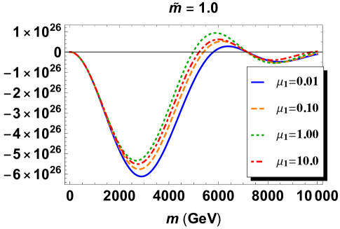
Figure 1: Spectrum of strange quark tower. $\det{\cal M}_{L}^{D}$ in Eq.  (5.45) is plotted as a function of $m=k\lambda$ for $\tilde{m}_{D}=1.0$ and various values of $\mu_{1}$. The mass spectrum $\{m_{n}=k\lambda_{n}\}$ is determined by roots of $\det{\cal M}_{L}^{D}=0$. $m_{\rm KK}=8062\,$GeV.

Case II: $c_{D^{+}}=-c_{D^{-}}=c_{D}$

The BCs at $z=z_{L}$ are given by

$$\left\{\begin{array}[]{l}d_{R}=0,\\ D_{+}(c_{Q})d_{L}=0,\\ D_{-}(c_{Q})d_{R}^{\prime}=0,\\ d_{L}^{\prime}=0,\\ \end{array}\right.\ \ \ \left\{\begin{array}[]{l}D_{R}^{+}=0,\\ D_{+}(c_{D})D_{L}^{+}=0,\\ D_{+}(c_{D})D_{R}^{-}=0,\\ D_{L}^{-}=0.\\ \end{array}\right.$$ (5.69)

In the twisted gauge, the BCs in Eq. (5.69) are satisfied by mode functions in (B.13) and (B.102) so that one can write as

$$\begin{pmatrix}\widetilde{\check{d}}_{R}\cr\widetilde{\check{d^{\prime}}}_{R}\cr\widetilde{\check{D}}{}_{R}^{+}\cr\widetilde{\check{D}}{}_{R}^{-}\end{pmatrix} =\begin{pmatrix}\alpha_{d}S_{R}(z;\lambda,c_{Q})\cr\kern 4.0pt\cr\alpha_{d^{\prime}}C_{R}(z;\lambda,c_{Q})\cr\kern 4.0pt\cr a_{d}\hat{\cal S}_{R2}(z;\lambda,c_{D},\tilde{m}_{D})+b_{d}\hat{\cal S}_{R1}(z;\lambda,c_{D},\tilde{m}_{D})\cr\kern 4.0pt\cr a_{d}\hat{\cal C}_{L1}(z;\lambda,c_{D},\tilde{m}_{D})+b_{d}\hat{\cal C}_{L2}(z;\lambda,c_{D},\tilde{m}_{D})\cr\end{pmatrix},$$ (5.70)

$$\begin{pmatrix}\widetilde{\check{d}}_{L}\cr\widetilde{\check{d^{\prime}}}_{L}\cr\widetilde{\check{D}}{}_{L}^{+}\cr\widetilde{\check{D}}{}_{L}^{-}\end{pmatrix} =\begin{pmatrix}\alpha_{d}C_{L}(z;\lambda,c_{Q})\cr\kern 4.0pt\cr\alpha_{d^{\prime}}S_{L}(z;\lambda,c_{Q})\cr\kern 4.0pt\cr a_{d}\hat{\cal C}_{L2}(z;\lambda,c_{D},\tilde{m}_{D})+b_{d}\hat{\cal C}_{L1}(z;\lambda,c_{D},\tilde{m}_{D})\cr\kern 4.0pt\cr-a_{d}\hat{\cal S}_{R1}(z;\lambda,c_{D},\tilde{m}_{D})-b_{d}\hat{\cal S}_{R2}(z;\lambda,c_{D},\tilde{m}_{D})\cr\end{pmatrix},$$ (5.71)

where $\alpha_{d}$, $\alpha_{d^{\prime}}$, $a_{d}$, $b_{d}$ are parameters.

From Eqs. (5.22) and (5.26), we find the boundary conditions at $z=1$ for the left-handed fields. The manipulation is similar to that in Case I. The difference appears only for terms involving $D_{L/R}^{-}$. It is straightforward to see

$${\cal M}_{L}^{D}\,V^{D}=\begin{pmatrix}\cos\frac{\theta_{H}}{2}S_{R}^{Q}&-i\sin\frac{\theta_{H}}{2}C_{R}^{Q}&0&0\\ -i\sin\frac{\theta_{H}}{2}C_{L}^{Q}&\cos\frac{\theta_{H}}{2}S_{L}^{Q}&\mu_{1}\hat{\cal C}_{L2}^{D}&\mu_{1}\hat{\cal C}_{L1}^{D}\\ -i\mu_{1}^{*}\sin\frac{\theta_{H}}{2}S_{R}^{Q}&\mu_{1}^{*}\cos\frac{\theta_{H}}{2}C_{R}^{Q}&-\hat{\cal S}_{R2}^{D}&-\hat{\cal S}_{R1}^{D}\\ 0&0&\hat{\cal S}_{R1}^{D}&\hat{\cal S}_{R2}^{D}\\ \end{pmatrix}\begin{pmatrix}\alpha_{d}\\ \alpha_{d^{\prime}}\\ a_{d}\\ b_{d}\\ \end{pmatrix}=0$$ (5.72)

where $S_{L/R}^{Q}:=S_{L/R}(z=1;\lambda,c_{Q})$, $\hat{\cal S}_{L/Rj}^{D}=\hat{\cal S}_{L/Rj}(z=1;\lambda,c_{D},\tilde{m}_{D})$ etc.. The spectrum is determined by

$$\det{\cal M}_{L}^{D}=\Big{(}S_{L}^{Q}S_{R}^{Q}+\sin^{2}\frac{\theta_{H}}{2}\Big{)}\Big{\{}(\hat{\cal S}_{R1}^{D})^{2}-(\hat{\cal S}_{R2}^{D})^{2}\Big{\}}$$ (5.73)

$$\hskip 85.35826pt+|\mu_{1}|^{2}C_{R}^{Q}S_{R}^{Q}(\hat{\cal S}_{R1}^{D}\hat{\cal C}_{L1}^{D}-\hat{\cal S}_{R2}^{D}\hat{\cal C}_{L2}^{D})=0~{}.$$ (5.74)

Note the relation (B.80).

For $|c_{Q}|,\hat{c}>\hbox{$\frac{1}{2}$}$ , $c_{D}>0$ and $\lambda z_{L}\ll 1$, we have

$$S_{L}^{Q}S_{R}^{Q}+\sin^{2}\frac{\theta_{H}}{2}\simeq-\frac{(\lambda^{2}-\lambda_{u}^{2})z_{L}^{2|c_{Q}|+1}}{4c_{Q}^{2}-1}~{},$$ (5.75)

$$(\hat{\cal S}_{R1}^{D})^{2}-(\hat{\cal S}_{L2}^{D})^{2}\sim-\alpha_{+}^{2}z_{L}^{2\hat{c}}~{},$$ (5.76)

$$\hat{\cal S}_{R1}^{D}{\cal C}_{L1}^{D}-\hat{\cal S}_{R2}^{D}{\cal C}_{L2}^{D}\sim(1+\alpha_{+}^{2})\,\frac{\lambda z_{L}^{2\hat{c}}}{2\hat{c}-1}~{},$$ (5.77)

so that

$$\det{\cal M}_{L}^{D}\simeq-\frac{(\lambda^{2}-\lambda_{u}^{2})z_{L}^{2|c_{Q}|+1}}{4c_{Q}^{2}-1}\cdot\left(-\alpha_{+}^{2}z_{L}^{2\hat{c}}\right)$$ (5.78)

$$\hskip 28.45274pt+|\mu_{1}|^{2}\left\{\begin{array}[]{c}\displaystyle\frac{1}{2c_{Q}-1}\\ \kern 5.0pt\cr\displaystyle\frac{z_{L}^{2|c_{Q}|+1}}{2|c_{Q}|+1}\\ \end{array}\right\}(1+\alpha_{+}^{2})\frac{\lambda^{2}z_{L}^{2\hat{c}}}{2\hat{c}+1}=0\ \ \mbox{for}\ \ \left\{\begin{array}[]{l}c_{Q}>\hbox{$\frac{1}{2}$}\\ \kern 10.0pt\cr c_{Q}<-\hbox{$\frac{1}{2}$}\\ \end{array}\right..$$ (5.83)

Thus we find

$$\lambda^{2}\left[1+\frac{|\mu_{1}|^{2}}{2\hat{c}-1}\left\{\begin{array}[]{c}\displaystyle(2c_{Q}+1)z_{L}^{-2|c_{Q}|-1}\\ \kern 5.0pt\cr\displaystyle 2|c_{Q}|-1\\ \end{array}\right\}\frac{1+\alpha_{+}^{2}}{\alpha_{+}^{2}}\right]=\lambda_{u}^{2}\ \ \mbox{for}\ \ \left\{\begin{array}[]{l}c_{Q}>\hbox{$\frac{1}{2}$}\\ \kern 5.0pt\cr c_{Q}<-\hbox{$\frac{1}{2}$}\\ \end{array}\right..$$ (5.88)

We observe that $\lambda^{2}<\lambda_{u}^{2}$ so that $m_{d}>m_{u}$ cannot be realized with this parametrization, as in Case I.

5.3 Charged lepton

$Q_{\rm EM}=-1$: $e,e^{\prime}$ $(\Psi_{({\bf 1,4})})$

In general $\Psi_{({\bf 1,4})}$ may couple with $\Psi_{({\bf 1,5})}^{\pm}$ through the brane interaction ${\cal L}_{2}^{m}$ in (3.42). We suppose that $\tilde{\mu}_{2}$ there is sufficiently small so that the effect of ${\cal L}_{2}^{m}$ can be ignored. In this case the equations and boundary conditions for $e,e^{\prime}$ take the same form as those for $u,u^{\prime}$. Mode functions and boundary conditions are summarized as

$$\begin{pmatrix}\tilde{\check{e}}{}_{R}\cr\tilde{\check{e}}{}_{R}^{\prime}\end{pmatrix}=\begin{pmatrix}\alpha_{e}S_{R}(z,\lambda,c_{L})\cr\alpha_{e^{\prime}}C_{R}(z,\lambda,c_{L})\end{pmatrix},$$ (5.89)

$$\begin{pmatrix}\tilde{\check{e}}{}_{L}\cr\tilde{\check{e}}{}_{L}^{\prime}\end{pmatrix}=\begin{pmatrix}\alpha_{e}C_{L}(z,\lambda,c_{L})\cr\alpha_{e^{\prime}}S_{L}(z,\lambda,c_{L})\end{pmatrix},$$ (5.90)

$$\begin{pmatrix}\cos\hbox{$\frac{1}{2}$}\theta_{H}S_{R}^{L}&-i\sin\hbox{$\frac{1}{2}$}\theta_{H}C_{R}^{L}\cr-i\sin\hbox{$\frac{1}{2}$}\theta_{H}C_{L}^{L}&\cos\hbox{$\frac{1}{2}$}\theta_{H}S_{L}^{L}\end{pmatrix}\begin{pmatrix}\alpha_{e}\cr\alpha_{e^{\prime}}\end{pmatrix}=0~{},$$ (5.91)

where $S_{L/R}^{L}=S_{L/R}(1,\lambda,c_{L})$ etc. in the last equation. The mass spectrum is determined by

$$S_{L}^{L}S_{R}^{L}+\sin^{2}\frac{\theta_{H}}{2}=0~{}.$$ (5.92)

The mass of the lowest mode (charged lepton) $m=k\lambda$ is given by

$$m_{e}=\pi^{-1}\sqrt{4c_{L}^{2}-1}\,z_{L}^{-|c_{L}|+0.5}\sin\hbox{$\frac{1}{2}$}\theta_{H}\,m_{\rm KK}~{}.$$ (5.93)

Note $|c_{L}|>\hbox{$\frac{1}{2}$}$.

5.4 Neutrino

$Q_{\rm EM}=0$: $\nu,\nu^{\prime},\chi$ $(\Psi_{({\bf 1,4})(-3)},\chi)$

As mentioned above, we assume that ${\cal L}_{2}^{m}$ can be ignored. The brane interaction ${\cal L}_{3}$ in (3.37) yields the coupling between $\nu^{\prime}$ and $\chi$, ${\cal L}_{3}^{m}$ in (3.42). It leads to the gauge-Higgs seesaw mechanism.[35] In the present paper we treat the case in which all brane interactions are diagonal in generations. In particular we set $M^{\alpha\beta}=-M_{\alpha}\delta^{\alpha\beta}$ in (3.42).

Equations of motion are given by

$$\begin{matrix}(a)\cr(b)\end{matrix}:\quad-i\delta\begin{pmatrix}\nu_{L}^{{\dagger}}\cr\nu_{L}^{\prime{\dagger}}\end{pmatrix}:\ -k\hat{D}_{-}(c_{L})\begin{pmatrix}\check{\nu}_{R}\cr\check{\nu}_{R}^{\prime}\end{pmatrix}+\sigma^{\mu}\partial_{\mu}\begin{pmatrix}\check{\nu}_{L}\cr\check{\nu}_{L}^{\prime}\end{pmatrix}=0~{},$$ (5.94)

$$\begin{matrix}(c)\cr(d)\end{matrix}:\quad\hskip 6.99997pti\delta\begin{pmatrix}\nu_{R}^{{\dagger}}\cr\nu_{R}^{\prime{\dagger}}\end{pmatrix}:\ \overline{\sigma}^{\mu}\partial_{\mu}\begin{pmatrix}\check{\nu}_{R}\cr\check{\nu}_{R}^{\prime}\end{pmatrix}-k\hat{D}_{+}(c_{L})\begin{pmatrix}\check{\nu}_{L}\cr\check{\nu}_{L}^{\prime}\end{pmatrix}=\frac{2m_{B}}{\sqrt{k}}\,\delta(y)\begin{pmatrix}0\cr\eta\end{pmatrix},$$ (5.95)

$$(e):\quad\hskip 18.99995pti\delta\eta^{\dagger}~{}~{}:\ \Big{\{}{\sigma}^{\mu}\partial_{\mu}\eta-\frac{m_{B}}{\sqrt{k}}\nu_{R}^{\prime}+M\eta^{c}\Big{\}}\,\delta(y)=0~{}.$$ (5.96)

$\nu_{R}$ and $\nu_{L}^{\prime}$ are parity-odd at $y=0$, whereas $\nu_{L}$ and $\nu_{R}^{\prime}$ are parity-even. We integrate the equations $(a)$, $(d)$ in the vicinity of $y=0$ and evaluate the equations $(b)$, $(c)$ at $y=+{\epsilon}$ to find boundary conditions at $y=+{\epsilon}$ as

$$(a)\ \Rightarrow\ \check{\nu}_{R}(x,\epsilon)=0~{},$$ (5.97)

$$(d)\ \Rightarrow\ -\check{\nu}_{L}^{\prime}(x,\epsilon)=+\frac{m_{B}}{\sqrt{k}}\,\eta(x)~{},$$ (5.98)

$$(b)\ \Rightarrow\ -\hat{D}_{-}(c_{L})\check{\nu}_{R}^{\prime}-\frac{m_{B}^{2}}{k^{2}}\check{\nu}_{R}^{\prime}+\frac{m_{B}M}{k^{3/2}}\eta^{c}=0~{},$$ (5.99)

$$(c)\ \Rightarrow\ \hat{D}_{+}(c_{L})\check{\nu}_{L}=0~{}.$$ (5.100)

Boundary conditions at $z=z_{L}$ are given by ${D}_{+}(c_{L})\check{\nu}_{L}=\check{\nu}_{R}=0$ and $\check{\nu}_{L}^{\prime}={D}_{-}(c_{L})\check{\nu}_{R}^{\prime}=0$.

Mode functions of these fields in the twisted gauge can be written as

$$\begin{pmatrix}\tilde{\check{\nu}}_{R}\cr\tilde{\check{\nu}}_{R}^{\prime}\cr\eta^{c}\end{pmatrix}=\begin{pmatrix}\alpha_{\nu}S_{R}^{L}\cr i\alpha_{\nu^{\prime}}C_{R}^{L}\cr\mp i\alpha_{\eta}^{*}/\sqrt{k}\end{pmatrix}f_{\pm R}(x)~{},~{}\begin{pmatrix}\tilde{\check{\nu}}_{L}\cr\tilde{\check{\nu}}_{L}^{\prime}\cr\eta\end{pmatrix}=\begin{pmatrix}\alpha_{\nu}C_{L}^{L}\cr i\alpha_{\nu^{\prime}}S_{L}^{L}\cr i\alpha_{\eta}/\sqrt{k}\end{pmatrix}f_{\pm L}(x)~{},$$ (5.101)

$$\bar{\sigma}^{\mu}\partial_{\mu}f_{\pm R}(x)=k\lambda f_{\pm L}(x)~{},~{}~{}{\sigma}^{\mu}\partial_{\mu}f_{\pm L}(x)=k\lambda f_{\pm R}(x)~{},$$ (5.102)

$$f_{\pm L}(x)^{c}=e^{i\delta_{C}}\sigma^{2}f_{\pm L}(x)^{*}=\pm f_{\pm R}(x)$$ (5.103)

where $S_{L/R}^{L}=S_{L/R}(z;\lambda,c_{L})$ and $C_{L/R}^{L}=C_{L/R}(z;\lambda,c_{L})$, and $\delta_{C}$ is defined in Eq. (3.33). Explicit forms of $f_{\pm L/R}$ are given in Appendix C. One can take $\alpha_{\nu},\alpha_{\nu^{\prime}},\alpha_{\eta}$ to be real. In this case $\sigma^{\mu}\partial_{\mu}\eta=\mp k\lambda\eta^{c}$ is satisfied so that the equation $(e)$ in Eq. (5.96) implies that

$$\frac{m_{B}}{\sqrt{k}}\,\check{\nu}_{R}^{\prime}\Big{|}_{y=0}-(M\mp k\lambda)\eta^{c}=0~{}.$$ (5.104)

With this identity the third relation in Eq. (5.100) can be rewritten as

$$\hat{D}_{-}(c_{L})\check{\nu}_{R}^{\prime}\mp\frac{m_{B}\lambda}{\sqrt{k}}\,\eta^{c}=0~{}.$$ (5.105)

Substituting (5.103) into (5.100), one finds

$$K_{\nu}\begin{pmatrix}\alpha_{\nu}\cr\alpha_{\nu^{\prime}}\cr\alpha_{\eta}\end{pmatrix}=\begin{pmatrix}\cos\frac{\theta_{H}}{2}S_{R}^{L}&\sin\frac{\theta_{H}}{2}C_{R}^{L}&0\cr\kern 5.0pt\cr-\sin\frac{\theta_{H}}{2}C_{L}^{L}&\cos\frac{\theta_{H}}{2}S_{L}^{L}&\frac{\displaystyle m_{B}}{\displaystyle k}\cr\kern 5.0pt\cr m_{B}\sin\frac{\theta_{H}}{2}S_{R}^{L}&-m_{B}\cos\frac{\theta_{H}}{2}C_{R}^{L}&k\lambda\mp M\end{pmatrix}\begin{pmatrix}\alpha_{\nu}\cr\alpha_{\nu^{\prime}}\cr\alpha_{\eta}\end{pmatrix}=0$$ (5.106)

where $S_{L/R}^{L}=S_{L/R}(1;\lambda,c_{L})$ etc.. From $\det K_{\nu}=0$, we find the mass spectrum formula for the neutrino sector:

$$\det K_{\nu}=(k\lambda\pm M)\Big{\{}S_{L}^{L}S_{R}^{L}+\sin^{2}\frac{\theta_{H}}{2}\Big{\}}+\frac{m_{B}^{2}}{k}S_{R}^{L}C_{R}^{L}=0~{}.$$ (5.107)

One of the solutions with $f_{+R/L}(x)$ or $f_{-R/L}(x)$ allows a small mass eigenvalue $m_{\nu}=k\lambda_{\nu}>0$. For $M>0$, the neutrino mode is obtained with $f_{+R/L}(x)$. Noting $\lambda z_{L}\ll 1$ and $k\lambda\ll M$, one finds the neutrino mass given by

$$m_{\nu}\simeq\begin{cases}\frac{\displaystyle m_{e}^{2}Mz_{L}^{2c_{L}+1}}{\displaystyle(2c_{L}+1)m_{B}^{2}}&{\rm for~{}}c_{L}>\hbox{$\frac{1}{2}$}~{},\cr\kern 5.0pt\cr\frac{\displaystyle m_{e}^{2}M}{\displaystyle(2|c_{L}|-1)m_{B}^{2}}&{\rm for~{}}c_{L}<-\hbox{$\frac{1}{2}$}~{}.\end{cases}$$ (5.108)

The gauge-Higgs seesaw mechanism[35, 42, 43] is characterized by a $3\times 3$ mass matrix

$$\frac{i}{2}(\nu_{0L}^{c\dagger},\nu_{0R}^{\prime\dagger},\eta^{c\dagger})\begin{pmatrix}0&m_{e}&0\cr m_{e}&0&\tilde{m}_{B}\cr 0&\tilde{m}_{B}&M\end{pmatrix}\begin{pmatrix}\nu_{0L}\cr\nu_{0R}^{\prime c}\cr\eta\end{pmatrix}+{h.c.}~{},$$ (5.109)

where $m_{e}$ is its corresponding charged lepton mass. The structure takes the same form as the inverse seesaw mechanism in Ref. [43], and yields very light neutrino mass $m_{\nu}\sim m_{e}^{2}M/\tilde{m}_{B}^{2}$. The Majorana mass $M$ may take a moderate value. In particular, for $c_{L}<-\hbox{$\frac{1}{2}$}$, $m_{\nu}\sim 1\,$meV is obtained with $m_{B}\sim 1\,$TeV and $M\sim 50\,$GeV. For $c_{L}>\hbox{$\frac{1}{2}$}$, $m_{B}$ has to take a rather large value, larger than the Planck mass.

Table 7: Parameters which reproduce the spectrum of leptons for $\theta_{H}=0.15$, $z_{L}=10^{10}$. $m_{\rm KK}=8.062\,$TeV. The masses of the 1st KK modes leptons are also shown in the unit of TeV. For $c_{L}>0$, there appear light neutrino excitation modes, $\nu_{s}$. The values $m_{e}=0.511\,$MeV, $m_{\mu}=105.7\,$MeV, $m_{\tau}=1.776\,$GeV, and $m_{\nu}=1\,$meV have been used.

Leptons	$c_{L}$	$M$	$m_{B}$	$m_{\nu_{s}}$	$m_{\nu^{(1)}}$	$m_{e^{(1)}}$
		(GeV)	(GeV)		(TeV)	(TeV)
$(\nu_{e},e)$	$1.086$	$10^{3}$	$6.6\times 10^{19}$	$6.8\,$MeV	$8.38$	$8.38$
		$1$	$2.1\times 10^{18}$	$6.8\,$MeV	$8.38$	$8.38$
	$-1.086$	$10^{3}$	$1.5\times 10^{4}$	–	$8.38$	$8.38$
		$1$	$4.7\times 10^{2}$	–	$0.51$	$8.38$
$(\nu_{\mu},\mu)$	$0.839$	$10^{3}$	$5.0\times 10^{19}$	$1.4\,$GeV	7.47	$7.47$
	$-0.839$	$10^{3}$	$1.2\times 10^{7}$	–	$7.47$	$7.47$
$(\nu_{\tau},\tau)$	$0.703$	$10^{3}$	$3.9\times 10^{19}$	$24.\,$GeV	6.96	$6.96$
	$-0.703$	$10^{3}$	$8.8\times 10^{8}$	–	6.96	$6.96$

Typical parameters in the lepton sector are summarized in Table 7. $|c_{L}|$ and $m_{e^{(1)}}$ are fixed by $m_{e}$. The value of $M$ can be varied. The spectrum does not depend on $M$ very much. As is seen in the table, very light neutrino excited mode $\nu_{s}$ appears for positive $c_{L}$. This does not necessarily mean the inconsistency with the observation. The $\nu_{s}$ mode may become a candidate for warm dark matter,[44] though more detailed investigation of gauge couplings is necessary to see the feasibility. For negative $c_{L}$ very light neutrino excited mode appears only when $M$ becomes very small. The spectrum of the neutrino towers are shown in fig. 2 for $c_{L}>0$ and in fig. 3 for $c_{L}<0$.

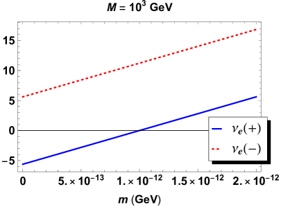
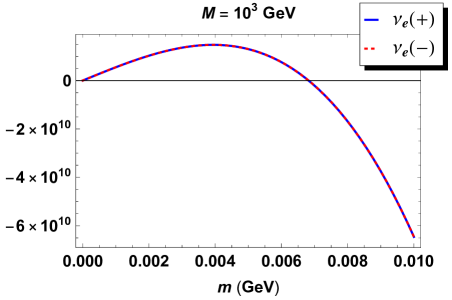
(a)                                                             (b)

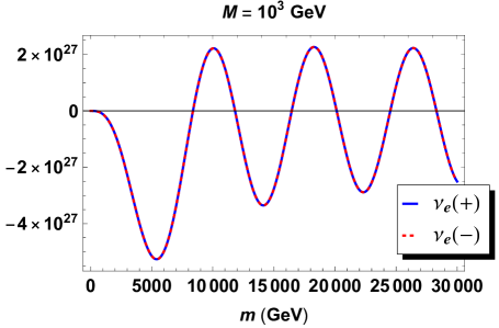
(c)

Figure 2: Spectrum of electron neutrino tower for $c_{e}>0$. $\det K_{\nu}$ in (5.107) is plotted as a function of $m=k\lambda$ in various mass ranges for $\theta_{H}=0.15$, $z_{L}=10^{10}$, $m_{\rm KK}=8.062\,$TeV and $M=1\,$TeV. The mass spectrum $\{m_{n}=k\lambda_{n}\}$ is determined by roots of $\det K_{\nu}=0$. $\nu_{e}(\pm)$ indicates the case of $f_{\pm L/R}(x)$ in (5.103). Only $\nu_{e}(+)$ has a solution corresponding to $\nu_{e}$ with $m_{\nu_{e}}=1\,$meV. In (b) and (c) the curves for $\nu_{e}(+)$ and $\nu_{e}(-)$ almost overlap with each other at this scale.

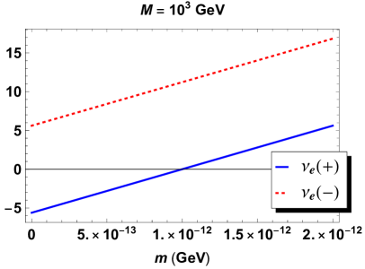
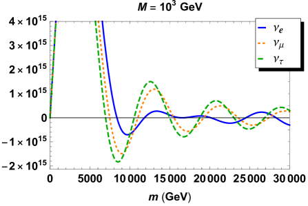
(a)                                                             (b)

Figure 3: Spectrum of neutrino towers for $c_{L}<0$. As in Fig. 2, $\det K_{\nu}$ in (5.107) is plotted as a function of $m=k\lambda$ in two mass ranges for $\theta_{H}=0.15$, $z_{L}=10^{10}$, $m_{\rm KK}=8.062\,$TeV and $M=1\,$TeV. The mass spectrum $\{m_{n}=k\lambda_{n}\}$ is determined by roots of $\det K_{\nu}=0$. (a) Only $\nu_{e}(+)$ has a solution corresponding to $\nu_{e}$ with $m_{\nu_{e}}=1\,$meV. (b) The spectrum of $\nu_{e},\nu_{\mu},\nu_{\tau}$ towers are shown. $\nu(+)$ and $\nu(-)$ towers almost overlap in this figure. For the $\nu_{e}$ tower the masses of the 3rd and 4th KK modes are 16.46 TeV and 16.67 TeV, respectively.

5.5 $W$ couplings of quarks and leptons

As have been shown above, the quark and lepton mass spectrum can be reproduced except that the down quark mass turns out lighter than the up quark mass. At this stage one might worry about the $W$ couplings of quarks and leptons in the current scheme. In the gauge-Higgs unification the $W$ boson at $\theta_{H}\not=0$ necessarily contains the original $SU(2)_{R}$ component as seen in Section 4.1. If quarks and leptons originated from only spinor representation multiplets in $SO(5)$, right-handed components of quarks and leptons also would have had non-vanishing couplings to $W$, which contradicts with the observation.

The left-handed quark and lepton doublets are mainly in the spinor representation of $SO(5)$, which have nominal $W$ couplings. The mechanism in the current model for making right-handed quarks and leptons having almost vanishing $W$ couplings is the following. The up-type quarks are contained solely in the spinor multiplets. The down-type quarks are contained in both of the spinor and singlet representations of $SO(5)$. Left-handed down-type quarks are mostly in the spinor representation multiplets, whereas right-handed down-type quarks are mostly in the singlet representation multiplets so that right-handed up-type quarks have almost vanishing $W$ couplings to right-handed down-type quarks.

The mechanism in the lepton sector is different. With the presence of brane fermions $\chi$, the gauge-Higgs seesaw mechanism functions in the neutrino sector. Right-handed neutrinos become heavy, acquiring $O(m_{\rm KK})$ masses, and decouple from right-handed charged leptons.

Indeed, one can evaluate the $W$ couplings of quarks and leptons by determining wave functions of quarks and leptons from the mass-determining matrices explained above and inserting them to the original action. The result is shown in Table 8. It is seen that the $\mu$-$e$ universality in the charged current interactions holds to high accuracy, provided the same sign of $c_{L}$ is adopted. It is also confirmed that the $W$ couplings of right-handed quarks and leptons are strongly suppressed. More detailed study of gauge couplings, including $Z$ and $Z^{\prime}$ couplings, will be given separately.

Table 8: $W$ couplings of quarks and leptons for $\theta_{H}=0.15$, $z_{L}=10^{10}$. $m_{\rm KK}=8.062\,$TeV. The couplings are defined by ${\cal L}=W_{\mu}\big{(}g_{L}^{W}\bar{u}_{L}\gamma^{\mu}d_{L}+g_{R}^{W}\bar{u}_{R}\gamma^{\mu}d_{R})$ for $(u,d)$ doublet. In the SM $g_{L}^{W}=g_{w}/\sqrt{2}$ and $g_{R}^{W}=0$. For $(u,d)$ doublet, we set $m_{d}=0.9\,m_{u}$.

Leptons	$c_{L}$	$M$	$\frac{\displaystyle g_{L}^{W}}{\displaystyle g_{w}/\sqrt{2}}-1$	$\frac{\displaystyle g_{R}^{W}}{\displaystyle g_{w}/\sqrt{2}}$
$(\nu_{e},e)$	$1.086$	$1\,$TeV	$-2.64\times 10^{-3}$	$O(10^{-11})$
	$-1.086$	$1\,$TeV	$-5.24\times 10^{-3}$	$O(10^{-23})$
$(\nu_{\mu},\mu)$	$0.839$	$1\,$TeV	$-2.64\times 10^{-3}$	$O(10^{-14})$
	$-0.839$	$1\,$TeV	$-5.25\times 10^{-3}$	$O(10^{-21})$
$(\nu_{\tau},\tau)$	$0.703$	$1\,$TeV	$-2.64\times 10^{-3}$	$O(10^{-15})$
	$-0.703$	$1\,$TeV	$-5.25\times 10^{-3}$	$O(10^{-19})$

Quarks	$c_{Q}$	$\mu_{1}$	$\tilde{m}_{D}$	$\frac{\displaystyle g_{L}^{W}}{\displaystyle g_{w}/\sqrt{2}}-1$	$\frac{\displaystyle g_{R}^{W}}{\displaystyle g_{w}/\sqrt{2}}$
$(u,d)$	$-1.044$	$0.1$	$1.0$	$-5.24\times 10^{-3}$	$O(10^{-14})$
$(c,s)$	$-0.7546$	$0.1$	$1.0$	$-5.25\times 10^{-3}$	$O(10^{-9})$
$(t,b)$	$0.2287$	$0.1$	$0.1$	$-3.43\times 10^{-3}$	$O(10^{-4})$
	$-0.2287$	$0.1$	$1.0$	$-4.41\times 10^{-3}$	$O(10^{-5})$

6 Summary and discussions

In this paper we have presented a new model of the $SO(5)\times U(1)\times SU(3)$ gauge-Higgs unification in which quark and lepton multiplets are introduced in the spinor, vector, and singlet representations of $SO(5)$ such that they can be implemented in the $SO(11)$ gauge-Higgs grand unification scheme. This should be contrasted to the previous model in which all quark and lepton multiplets are introduced in the vector representation of $SO(5)$. The up-type quarks are contained solely in the spinor representation. The right-handed down-type quarks are mainly contained in the singlet representation of $SO(5)$. $SO(5)\times U(1)\times SU(3)$ singlet brane Majorana fermions are introduced on the UV brane. The coupling of these brane fermions to bulk fermion multiplets induces the gauge-Higgs seesaw mechanism in the neutrino sector, which takes the same form as the inverse seesaw mechanism in four-dimensional GUT theories.

With $SO(5)\times U(1)\times SU(3)$ gauge-invariant brane interactions taken into account the quark-lepton mass spectrum has been reproduced with the exception that down quark mass ($m_{d}$) becomes lighter than up quark mass ($m_{u}$). A solution to this problem is yet to be found. The compatibility with grand unification severely restricts matter content and interactions in the gauge-Higgs unification. Nevertheless it is very encouraging that the model yields almost the same $W$ couplings of quarks and leptons.

The present model serves as a viable alternative to the standard model. If it is the case, phenomenological consequences of the model need to be clarified. As in the previous model $Z^{\prime}$ bosons (the first KK modes of $\gamma$, $Z$ and $Z_{R}$) are predicted around $7\,$TeV to $10\,$TeV range. We have seen in Section 5 that the bulk mass parameters ($c_{u},c_{c}$) of quark multiplets $\Psi_{({\bf 3,4})}$ in the first and second generations must be negative to avoid exotic light excitation modes of down-quark-type. The bulk mass parameters $c_{L}$ of lepton multiplets can be either positive or negative. The sign of the bulk mass parameters is critically important to determine the behavior of wave functions. For $c>+\hbox{$\frac{1}{2}$}$ ($c<-\hbox{$\frac{1}{2}$})$ left-handed quarks/leptons are localized near the UV (IR) brane, whereas right-handed ones near the IR (UV) brane. As $Z^{\prime}$ bosons are localized near the IR brane, right-handed (left-handed) quarks/leptons have larger couplings to $Z^{\prime}$ bosons for $c>+\hbox{$\frac{1}{2}$}$ ($c<-\hbox{$\frac{1}{2}$})$. The effect of the large parity violation can be seen in the $e^{+}e^{-}$ collisions through interference terms. In particular, cross sections of various fermion-pair production processes should reveal distinct dependence on the $e^{-}$ polarization.[14]

With the mass spectra of all fields having been determined, one can investigate the effective potential $V_{\rm eff}(\theta_{H})$ to show that EW symmetry is dynamically broken. The flavor mixing in the quark and lepton sectors and the dark matter are also among the problems to be solved in the gauge-Higgs unification scenario. We shall come back to these issues in the near future.

Appendix A $SO(5)$

The generators of $SO(5)$, $T_{jk}=-T_{kj}=T_{jk}^{\dagger}$ ($j,k=1,2,3,4,5$), satisfy the algebra

$$[T_{ij},T_{kl}]=i(\delta_{ik}T_{jl}-\delta_{il}T_{jk}+\delta_{jl}T_{ik}-\delta_{jk}T_{il}).$$ (A.1)

In the adjoint representation,

$$(T_{ij})_{pq}=-i(\delta_{ip}\delta_{jq}-\delta_{iq}\delta_{jp}),$$

$$\mbox{tr}(T_{jk}T_{lm})=2(\delta_{jl}\delta_{km}-\delta_{jm}\delta_{kl}),\hskip 10.00002pt\mbox{tr}(T_{jk})^{2}=2.$$ (A.2)

We take the following basis of $SO(5)$ Clifford algebra:

$$\{\Gamma_{j},\Gamma_{k}\}=2\delta_{jk}I_{4}~{},$$ (A.3)

$$\Gamma_{a}=\sigma^{a}\otimes\sigma^{1}\quad(a=1,2,3)~{},$$ (A.4)

$$\Gamma_{4}=\sigma^{0}\otimes\sigma^{2}~{},~{}~{}\Gamma_{5}=\sigma^{0}\otimes\sigma^{3}=-\Gamma_{1}\Gamma_{2}\Gamma_{3}\Gamma_{4}~{},$$ (A.5)

where $\sigma^{0}=I_{2}$ and $\{\sigma^{a}\}$ are Pauli matrices. In terms of $\Gamma_{j}$ the $SO(5)$ generators in the spinor representation are given by

$$T_{jk}=-\frac{i}{4}[\Gamma_{j},\Gamma_{k}]\hskip 8.5359pt\Big{(}=-\frac{i}{2}\Gamma_{j}\Gamma_{k}\quad\mbox{for}\ j\not=k\Big{)},$$

$$(T_{jk})^{2}=\frac{1}{4}I_{4}~{},~{}~{}\mbox{tr}(T_{jk})^{2}=1~{}.$$ (A.6)

The orbifold boundary conditions $P_{0},P_{1}$ in Eqs (3.4) break $SO(5)$ to $SO(4)\simeq SU(2)_{L}\times SU(2)_{R}$. The generators of the corresponding $SO(4)\simeq SU(2)_{L}\times SU(2)_{R}$ in the spinor representation are given by

$$\vec{T}_{L} =\frac{1}{2}\begin{pmatrix}T_{23}+T_{14}\cr T_{31}+T_{24}\cr T_{12}+T_{34}\end{pmatrix}=\frac{1}{2}\vec{\sigma}\otimes\begin{pmatrix}1&0\cr 0&0\end{pmatrix},$$ (A.7)

$$\vec{T}_{R} =\frac{1}{2}\begin{pmatrix}T_{23}-T_{14}\cr T_{31}-T_{24}\cr T_{12}-T_{34}\end{pmatrix}=\frac{1}{2}\vec{\sigma}\otimes\begin{pmatrix}0&0\cr 0&1\end{pmatrix}.$$ (A.8)

These generators become block-diagonal so that an $SO(5)$ spinor representation 4 can be decomposed into $({\bf 2,1})\oplus({\bf 1,2})$ of $SO(4)\simeq SU(2)_{L}\times SU(2)_{R}$ :

$$\Psi_{\bf 4}=\begin{pmatrix}\Psi_{({\bf 2,1})}\cr\Psi_{({\bf 1,2})}\end{pmatrix}.$$ (A.9)

In the representation (A.5) one finds that

$$\Gamma_{j}^{*}=(-1)^{j+1}\Gamma_{j},$$

$$R:=-i\Gamma_{2}\Gamma_{4}=R^{\dagger}=R^{-1}=\sigma^{2}\otimes\sigma^{3},$$

$$R\Gamma_{j}R=(-1)^{j+1}\Gamma_{j},\ \ \ R\Gamma_{j}^{*}R=\Gamma_{j},$$

$$RT_{jk}^{*}R=-T_{jk}.$$ (A.10)

It follows that for an $SO(5)$ spinor $\Psi_{\bf 4}$, the $R$-transformed one also transforms as 4.

$$\tilde{\Psi}_{\bf 4}:=iR\Psi_{\bf 4}^{*}~{},$$ (A.11)

$$\Psi_{\bf 4}^{\prime}=\bigg{(}1+\frac{i}{2}\epsilon_{jk}T_{jk}\bigg{)}\Psi_{\bf 4}\ \ \ \Rightarrow\ \ \ \tilde{\Psi}_{\bf 4}^{\prime}=\bigg{(}1+\frac{i}{2}\epsilon_{jk}T_{jk}\bigg{)}\tilde{\Psi}_{\bf 4}.$$ (A.12)

Its $SO(5)$ content is given by

$$\tilde{\Psi}_{\bf 4}=\begin{pmatrix}\tilde{\Psi}_{({\bf 2,1})}\cr\tilde{\Psi}_{({\bf 1,2})}\end{pmatrix}=\begin{pmatrix}i\sigma^{2}{\Psi}_{({\bf 2,1})}^{*}\cr-i\sigma^{2}{\Psi}_{({\bf 1,2})}^{*}\end{pmatrix}.$$ (A.13)

Appendix B Basis functions

We summarize basis functions in the RS space.

B.1 Gauge fields

We define

$$F_{\alpha,\beta}(u,v)\equiv J_{\alpha}(u)Y_{\beta}(v)-Y_{\alpha}(u)J_{\beta}(v)$$ (B.1)

where $J_{\alpha}(x)$ and $Y_{\alpha}(x)$ are Bessel functions of the 1st and 2nd kind, respectively. For gauge bosons $C=C(z;\lambda)$ and $S=S(z;\lambda)$ are defined as solutions of

$$-{\cal P}_{4}\begin{pmatrix}C\\ S\end{pmatrix}=\left(-\frac{d^{2}}{dz^{2}}+\frac{1}{z}\frac{d}{dz}\right)\begin{pmatrix}C\\ S\end{pmatrix}=\lambda^{2}\begin{pmatrix}C\\ S\end{pmatrix},$$ (B.2)

with boundary conditions $C=z_{L}$, $S=0$, $C^{\prime}=0$, and $S^{\prime}=\lambda$ at $z=z_{L}$. They are given by

$$C(z;\lambda) =+\frac{\pi}{2}\lambda zz_{L}F_{1,0}(\lambda z,\lambda z_{L}),$$ (B.3)

$$C^{\prime}(z;\lambda) =+\frac{\pi}{2}\lambda^{2}zz_{L}F_{0,0}(\lambda z,\lambda z_{L}),$$ (B.4)

$$S(z;\lambda) =-\frac{\pi}{2}\lambda zF_{1,1}(\lambda z,\lambda z_{L}),$$ (B.5)

$$S^{\prime}(z;\lambda) =-\frac{\pi}{2}\lambda^{2}zF_{0,1}(\lambda z,\lambda z_{L}).$$ (B.6)

We note that

$$-{\cal P}_{z}\begin{pmatrix}C^{\prime}\\ S^{\prime}\end{pmatrix} =\lambda^{2}\begin{pmatrix}C^{\prime}\\ S^{\prime}\end{pmatrix},$$ (B.7)

$$CS^{\prime}-SC^{\prime} =\lambda z~{}.$$ (B.8)

B.2 Massless fermion fields

For massless fermions in five dimensions we define

$$\begin{pmatrix}C_{L}\cr S_{L}\end{pmatrix}(z;\lambda,c) =\pm\frac{\pi}{2}\lambda\sqrt{zz_{L}}\,F_{c+\frac{1}{2},c\mp\frac{1}{2}}(\lambda z,\,\lambda z_{L})~{},$$ (B.9)

$$\begin{pmatrix}C_{R}\cr S_{R}\end{pmatrix}(z;\lambda,c) =\mp\frac{\pi}{2}\lambda\sqrt{zz_{L}}\,F_{c-\frac{1}{2},c\pm\frac{1}{2}}(\lambda z,\,\lambda z_{L})~{},$$ (B.10)

which satisfy

$$D_{+}\begin{pmatrix}C_{L}\\ S_{L}\end{pmatrix}=\lambda\begin{pmatrix}S_{R}\\ C_{R}\end{pmatrix},~{}~{}D_{-}\begin{pmatrix}C_{R}\\ S_{R}\end{pmatrix}=\lambda\begin{pmatrix}S_{L}\\ C_{L}\end{pmatrix},$$ (B.11)

$$C_{L}C_{R}-S_{L}S_{R}=1~{},$$ (B.12)

$$C_{R}=C_{L}=1~{},~{}~{}S_{R}=S_{L}=0~{},~{}~{}{\rm at~{}}z=z_{L}.$$ (B.13)

They also satisfy

$$C_{L}(z;\lambda,-c)=C_{R}(z;\lambda,c)~{},~{}~{}S_{L}(z;\lambda,-c)=-S_{R}(z;\lambda,c)~{}.$$ (B.14)

B.3 Massive fermion fields

As seen in (3.21), $\check{\Psi}_{({\bf 3},{\bf 1})}^{\pm\alpha}$ and $\check{\Psi}_{({\bf 1},{\bf 5})}^{\pm\beta}$ have additional pseudo-Dirac bulk mass terms in the action. To find basis functions for these massive fermions, we consider the action for $N^{\pm}$ fields given by

$$\int d^{4}x\int_{1}^{z_{L}}\frac{dz}{k}\Big{\{}\overline{\check{N}}{}^{+}{\cal D}_{0}(c_{+})\check{N}^{+}+\overline{\check{N}}{}^{-}{\cal D}_{0}(c_{-})\check{N}^{-}-\frac{k\tilde{m}}{z}\big{(}\overline{\check{N}}{}^{+}\check{N}^{-}+\overline{\check{N}}{}^{-}\check{N}^{+}\big{)}\Big{\}}$$ (B.15)

$$\hskip 56.9055pt\hbox{where~{}}{\cal D}_{0}(c)=\begin{pmatrix}-kD_{-}(c)&\sigma^{\mu}\partial_{\mu}\cr\bar{\sigma}^{\mu}\partial_{\mu}&-kD_{+}(c)\end{pmatrix}.$$ (B.16)

$\tilde{m}$ is dimensionless, and $k\tilde{m}$ corresponds to $m_{D}^{\alpha}$ and $m_{V}^{\beta}$ in (3.21).

To find eigenmodes with four-dimensional mass $k\lambda$, we write $\check{N}_{R}^{\pm}(x,z)=N_{\pm R}(z)f_{R}(x)$ and $\check{N}_{L}^{\pm}(x,z)=N_{\pm L}(z)f_{L}(x)$ as described below Eq. (5.8). Then $N_{\pm R}(z)$ and $N_{\pm L}(z)$ must satisfy

$$D_{-}(c_{\pm})N_{\pm R}-\lambda N_{\pm L}+\frac{\tilde{m}}{z}\,N_{\mp R}=0~{},$$ (B.17)

$$D_{+}(c_{\pm})N_{\pm L}-\lambda N_{\pm R}+\frac{\tilde{m}}{z}\,N_{\mp L}=0~{}.$$ (B.18)

Note

$$D_{\pm}(c)D_{\mp}(c)=-\frac{d^{2}}{dz^{2}}+\frac{c(c\mp 1)}{z^{2}}~{}.$$ (B.19)

We consider two cases; $c_{+}=c_{-}$ and $c_{+}=-c_{-}$.

B.3.1 Case I. $c_{+}=c_{-}=c$

It follows immediately from (B.18) that

$$D_{-}(c\pm\tilde{m})(N_{+R}\pm N_{-R}) =\lambda\left(N_{+L}\pm N_{-L}\right)~{},$$ (B.20)

$$D_{+}(c\pm\tilde{m})(N_{+L}\pm N_{-L}) =\lambda\left(N_{+R}\pm N_{-R}\right)~{}.$$ (B.21)

General solutions are given by

$$\begin{pmatrix}N_{\pm R}\cr N_{\pm L}\end{pmatrix}=a\begin{pmatrix}C_{R}^{c+\tilde{m}}\cr S_{L}^{c+\tilde{m}}\end{pmatrix}+b\begin{pmatrix}S_{R}^{c+\tilde{m}}\cr C_{L}^{c+\tilde{m}}\end{pmatrix}\pm a^{\prime}\begin{pmatrix}C_{R}^{c-\tilde{m}}\cr S_{L}^{c-\tilde{m}}\end{pmatrix}\pm b^{\prime}\begin{pmatrix}S_{R}^{c-\tilde{m}}\cr C_{L}^{c-\tilde{m}}\end{pmatrix}.$$ (B.22)

Here $C_{L/R}^{c\pm\tilde{m}}=C_{L/R}(z;\lambda,{c\pm\tilde{m}})$ and $S_{L/R}^{c\pm\tilde{m}}=S_{L/R}(z;\lambda,{c\pm\tilde{m}})$.

At this stage we define basis functions by

$${\cal C}_{R1}(z;\lambda,c,\tilde{m}) =C_{R}(z;\lambda,c+\tilde{m})+C_{R}(z;\lambda,c-\tilde{m})~{},$$ (B.23)

$${\cal C}_{R2}(z;\lambda,c,\tilde{m}) =S_{R}(z;\lambda,c+\tilde{m})-S_{R}(z;\lambda,c-\tilde{m})~{},$$ (B.24)

$${\cal S}_{L1}(z;\lambda,c,\tilde{m}) =S_{L}(z;\lambda,c+\tilde{m})+S_{L}(z;\lambda,c-\tilde{m})~{},$$ (B.25)

$${\cal S}_{L2}(z;\lambda,c,\tilde{m}) =C_{L}(z;\lambda,c+\tilde{m})-C_{L}(z;\lambda,c-\tilde{m})~{},$$ (B.26)

$${\cal C}_{L1}(z;\lambda,c,\tilde{m}) =C_{L}(z;\lambda,c+\tilde{m})+C_{L}(z;\lambda,c-\tilde{m})~{},$$ (B.27)

$${\cal C}_{L2}(z;\lambda,c,\tilde{m}) =S_{L}(z;\lambda,c+\tilde{m})-S_{L}(z;\lambda,c-\tilde{m})~{},$$ (B.28)

$${\cal S}_{R1}(z;\lambda,c,\tilde{m}) =S_{R}(z;\lambda,c+\tilde{m})+S_{R}(z;\lambda,c-\tilde{m})~{},$$ (B.29)

$${\cal S}_{R2}(z;\lambda,c,\tilde{m}) =C_{R}(z;\lambda,c+\tilde{m})-C_{R}(z;\lambda,c-\tilde{m})~{},$$ (B.30)

which satisfy the equations and boundary conditions

$$D_{-}(c)\begin{pmatrix}{\cal C}_{R1}\cr{\cal C}_{R2}\end{pmatrix}=\lambda\begin{pmatrix}{\cal S}_{L1}\cr{\cal S}_{L2}\end{pmatrix}-\frac{\tilde{m}}{z}\begin{pmatrix}{\cal S}_{R2}\cr{\cal S}_{R1}\end{pmatrix},$$ (B.31)

$$D_{-}(c)\begin{pmatrix}{\cal S}_{R1}\cr{\cal S}_{R2}\end{pmatrix}=\lambda\begin{pmatrix}{\cal C}_{L1}\cr{\cal C}_{L2}\end{pmatrix}-\frac{\tilde{m}}{z}\begin{pmatrix}{\cal C}_{R2}\cr{\cal C}_{R1}\end{pmatrix},$$ (B.32)

$$D_{+}(c)\begin{pmatrix}{\cal C}_{L1}\cr{\cal C}_{L2}\end{pmatrix}=\lambda\begin{pmatrix}{\cal S}_{R1}\cr{\cal S}_{R2}\end{pmatrix}-\frac{\tilde{m}}{z}\begin{pmatrix}{\cal S}_{L2}\cr{\cal S}_{L1}\end{pmatrix},$$ (B.33)

$$D_{+}(c)\begin{pmatrix}{\cal S}_{L1}\cr{\cal S}_{L2}\end{pmatrix}=\lambda\begin{pmatrix}{\cal C}_{R1}\cr{\cal C}_{R2}\end{pmatrix}-\frac{\tilde{m}}{z}\begin{pmatrix}{\cal C}_{L2}\cr{\cal C}_{L1}\end{pmatrix},$$ (B.34)

$${\cal S}_{Rj}={\cal S}_{Lj}=D_{-}(c)\,{\cal C}_{Rj}=D_{+}(c)\,{\cal C}_{Lj}=0\quad{\rm at~{}}z=z_{L}~{}.$$ (B.35)

Note also

$${\cal C}_{Rj}(z;\lambda,-c,\tilde{m})={\cal C}_{Lj}(z;\lambda,c,\tilde{m})~{},$$ (B.36)

$${\cal S}_{Rj}(z;\lambda,-c,\tilde{m})=-{\cal S}_{Lj}(z;\lambda,c,\tilde{m})~{},$$ (B.37)

$${\cal C}_{R/Lj}(z;\lambda,c,-\tilde{m})=(-1)^{j-1}\,{\cal C}_{R/Lj}(z;\lambda,c,\tilde{m})~{},$$ (B.38)

$${\cal S}_{R/Lj}(z;\lambda,c,-\tilde{m})=(-1)^{j-1}\,{\cal S}_{R/Lj}(z;\lambda,c,\tilde{m})~{}.$$ (B.39)

In the $\tilde{m}\rightarrow 0$ limit

$${\cal C}_{R1}\to 2C_{R}~{},~{}~{}{\cal S}_{R1}\to 2S_{R}~{},~{}~{}{\cal C}_{L1}\to 2C_{L}~{},~{}~{}{\cal S}_{L1}\to 2S_{L}~{},$$ (B.40)

$${\cal C}_{R2},~{}{\cal S}_{R2},~{}{\cal C}_{L2},~{}{\cal S}_{L2}\rightarrow 0~{}.$$ (B.41)

Two types of boundary conditions appear at $z=z_{L}$.

Type A:  $(N_{+R},N_{-R},N_{+L},N_{-L})=(+,-,-,+)$

When parity assignment at $y=L$ for $(N_{+R},N_{-R},N_{+L},N_{-L})$ is $(+,-,-,+)$, boundary conditions at $z=z_{L}$ become

$$D_{-}(c)N_{+R}=0~{},~{}~{}N_{+L}=0~{},$$ (B.42)

$$N_{-R}=0~{},~{}~{}D_{+}(c)N_{-L}=0~{}.$$ (B.43)

In this case $a=a^{\prime}$ and $b=-b^{\prime}$ in (B.22) and solutions can be written as

$$\begin{pmatrix}N_{+R}\cr N_{+L}\cr N_{-R}\cr N_{-L}\end{pmatrix}=a\begin{pmatrix}{\cal C}_{R1}(z;\lambda,c,\tilde{m})\cr{\cal S}_{L1}(z;\lambda,c,\tilde{m})\cr{\cal S}_{R2}(z;\lambda,c,\tilde{m})\cr{\cal C}_{L2}(z;\lambda,c,\tilde{m})\end{pmatrix}+b\begin{pmatrix}{\cal C}_{R2}(z;\lambda,c,\tilde{m})\cr{\cal S}_{L2}(z;\lambda,c,\tilde{m})\cr{\cal S}_{R1}(z;\lambda,c,\tilde{m})\cr{\cal C}_{L1}(z;\lambda,c,\tilde{m})\end{pmatrix},$$ (B.44)

where $a,b$ are arbitrary constants.

If $N$’s have the same parity assignment at $y=0$ as that at $y=L$, then (B.43) must be satisfied at $z=1$ as well. Substituting (B.44) into (B.43) and evaluating the conditions at $z=1$, one finds

$$\begin{pmatrix}{\cal S}_{L1}&{\cal S}_{L2}\cr{\cal S}_{R2}&{\cal S}_{R1}\end{pmatrix}\begin{pmatrix}a\cr b\end{pmatrix}=0$$ (B.45)

where ${\cal S}_{L1}={\cal S}_{L1}(1;\lambda,c,\tilde{m})$ etc.. The mass spectrum is determined by

$${\cal S}_{L1}{\cal S}_{R1}-{\cal S}_{L2}{\cal S}_{R2}=0~{}.$$ (B.46)

Note

$${\cal S}_{L1}{\cal S}_{R1}-{\cal S}_{L2}{\cal S}_{R2}+2={\cal C}_{L1}{\cal C}_{R1}-{\cal C}_{L2}{\cal C}_{R2}-2$$ (B.47)

$$\quad=S_{L}^{c+\tilde{m}}S_{R}^{c-\tilde{m}}+S_{L}^{c-\tilde{m}}S_{R}^{c+\tilde{m}}+C_{L}^{c+\tilde{m}}C_{R}^{c-\tilde{m}}+C_{L}^{c-\tilde{m}}C_{R}^{c+\tilde{m}}~{},$$ (B.48)

$${\cal S}_{L1}{\cal C}_{L1}-{\cal S}_{L2}{\cal C}_{L2}=2\left(S_{L}^{c+\tilde{m}}C_{L}^{c-\tilde{m}}+S_{L}^{c-\tilde{m}}C_{L}^{c+\tilde{m}}\right)~{}.$$ (B.49)

Type B:  $(N_{+R},N_{-R},N_{+L},N_{-L})=(-,+,+,-)$

When parity assignment at $y=L$ for $(N_{+R},N_{-R},N_{+L},N_{-L})$ is $(-,+,+,-)$, boundary conditions at $z=z_{L}$ become

$$N_{+R}=0~{},~{}~{}D_{+}(c)N_{+L}=0~{},$$ (B.50)

$$D_{-}(c)N_{-R}=0~{},~{}~{}N_{-L}=0~{}.$$ (B.51)

In this case $a=-a^{\prime}$ and $b=b^{\prime}$ in (B.22) and solutions can be written as

$$\begin{pmatrix}N_{+R}\cr N_{+L}\cr N_{-R}\cr N_{-L}\end{pmatrix}=a\begin{pmatrix}{\cal S}_{R2}(z;\lambda,c,\tilde{m})\cr{\cal C}_{L2}(z;\lambda,c,\tilde{m})\cr{\cal C}_{R1}(z;\lambda,c,\tilde{m})\cr{\cal S}_{L1}(z;\lambda,c,\tilde{m})\end{pmatrix}+b\begin{pmatrix}{\cal S}_{R1}(z;\lambda,c,\tilde{m})\cr{\cal C}_{L1}(z;\lambda,c,\tilde{m})\cr{\cal C}_{R2}(z;\lambda,c,\tilde{m})\cr{\cal S}_{L2}(z;\lambda,c,\tilde{m})\end{pmatrix},$$ (B.52)

where $a,b$ are arbitrary constants.

If $N$’s have the same parity assignment at $y=0$ as that at $y=L$, then (B.51) must be satisfied at $z=1$ as well. Substituting (B.52) into (B.51) and evaluating the conditions at $z=1$, one finds

$$\begin{pmatrix}{\cal S}_{R2}&{\cal S}_{R1}\cr{\cal S}_{L1}&{\cal S}_{L2}\end{pmatrix}\begin{pmatrix}a\cr b\end{pmatrix}=0~{}.$$ (B.53)

The mass spectrum is determined by

$${\cal S}_{L1}{\cal S}_{R1}-{\cal S}_{L2}{\cal S}_{R2}=0~{}.$$ (B.54)

B.3.2 Case II. $c_{+}=-c_{-}=c$

The special case $c_{+}=-c_{-}=c$ naturally emerges in the context of six-dimensional gauge-Higgs grand unification.[35] The bulk (vector) mass parameter $c$ appears there as a coefficient in the vector component $\gamma^{6}$, which becomes the bulk mass parameter in the RS space, $\pm c$, for 6D Weyl ($\gamma^{7}=\pm$) components. In this case Eq. (B.18) becomes

$$D_{-}(c)N_{+R}-\lambda N_{+L}+\frac{\tilde{m}}{z}N_{-R}=0~{},$$ (B.55)

$$D_{+}(c)N_{+L}-\lambda N_{+R}+\frac{\tilde{m}}{z}N_{-L}=0~{},$$ (B.56)

$$- D_{+}(c)N_{-R}-\lambda N_{-L}+\frac{\tilde{m}}{z}N_{+R}=0~{},$$ (B.57)

$$- D_{-}(c)N_{-L}-\lambda N_{-R}+\frac{\tilde{m}}{z}N_{+L}=0~{}.$$ (B.58)

To find solutions to Eqs. (B.58), we note that

$$\left\{-\frac{d^{2}}{dz^{2}}+\frac{c(c\mp 1)}{z^{2}}+\frac{\tilde{m}^{2}}{z^{2}}-\lambda^{2}\right\}N_{\pm R}-\frac{\tilde{m}}{z^{2}}N_{\mp R}=0~{}.$$ (B.59)

We seek solutions in the form $N_{+R}=f(z)$ and $N_{-R}=\alpha f(z)$. Solutions exist provided $-c-\alpha\tilde{m}=c-{\tilde{m}}/{\alpha}$ is satisfied, or $\alpha=\alpha_{\pm}$ where

$$\alpha_{\pm}=\frac{1}{\tilde{m}}(-c\pm\hat{c})~{},~{}~{}\alpha_{+}\alpha_{-}=-1~{},$$ (B.60)

$$\hat{c}=\sqrt{c^{2}+\tilde{m}^{2}}~{}.$$ (B.61)

With $\alpha=\alpha_{\pm}$, $f(z)$ satisfies

$$\big{\{}D_{\pm}(\hat{c})D_{\mp}(\hat{c})-\lambda^{2}\big{\}}f(z)=0~{}.$$ (B.62)

Hence general solutions are given by

$$\begin{pmatrix}N_{+R}\cr N_{-R}\end{pmatrix}=a\begin{pmatrix}C_{R}^{\hat{c}}\cr\alpha_{+}C_{R}^{\hat{c}}\end{pmatrix}+b\begin{pmatrix}S_{R}^{\hat{c}}\cr\alpha_{+}S_{R}^{\hat{c}}\end{pmatrix}+a^{\prime}\begin{pmatrix}C_{L}^{\hat{c}}\cr\alpha_{-}C_{L}^{\hat{c}}\end{pmatrix}+b^{\prime}\begin{pmatrix}S_{L}^{\hat{c}}\cr\alpha_{-}S_{L}^{\hat{c}}\end{pmatrix},$$ (B.63)

where $C_{L/R}^{\hat{c}}=C_{L/R}(z;\lambda,\hat{c})$ and $S_{L/R}^{\hat{c}}=S_{L/R}(z;\lambda,\hat{c})$.

To find the corresponding solutions for $N_{\pm L}$, we make use of the identities

$$D_{-}(c) =+D_{-}(\hat{c})-\frac{\tilde{m}\alpha_{+}}{z}=-D_{+}(\hat{c})-\frac{\tilde{m}\alpha_{-}}{z}~{},$$ (B.64)

$$D_{+}(c) =+D_{+}(\hat{c})-\frac{\tilde{m}\alpha_{+}}{z}=-D_{-}(\hat{c})-\frac{\tilde{m}\alpha_{-}}{z}$$ (B.65)

to find

$$\begin{pmatrix}N_{+L}\cr N_{-L}\end{pmatrix}=a\begin{pmatrix}S_{L}^{\hat{c}}\cr\alpha_{+}S_{L}^{\hat{c}}\end{pmatrix}+b\begin{pmatrix}C_{L}^{\hat{c}}\cr\alpha_{+}C_{L}^{\hat{c}}\end{pmatrix}-a^{\prime}\begin{pmatrix}S_{R}^{\hat{c}}\cr\alpha_{-}S_{R}^{\hat{c}}\end{pmatrix}-b^{\prime}\begin{pmatrix}C_{R}^{\hat{c}}\cr\alpha_{-}C_{R}^{\hat{c}}\end{pmatrix}.$$ (B.66)

Basis functions for Case II are defined as follows.

$$\hat{\cal C}_{R1}(z;\lambda,c,\tilde{m}) =C_{R}(z;\lambda,\hat{c})+\alpha_{+}^{2}C_{L}(z;\lambda,\hat{c})~{},$$ (B.67)

$$\hat{\cal C}_{R2}(z;\lambda,c,\tilde{m}) =\alpha_{+}\big{\{}S_{L}(z;\lambda,\hat{c})+S_{R}(z;\lambda,\hat{c})\big{\}}~{},$$ (B.68)

$$\hat{\cal S}_{L1}(z;\lambda,c,\tilde{m}) =S_{L}(z;\lambda,\hat{c})-\alpha_{+}^{2}S_{R}(z;\lambda,\hat{c})~{},$$ (B.69)

$$\hat{\cal S}_{L2}(z;\lambda,c,\tilde{m}) =\alpha_{+}\big{\{}C_{L}(z;\lambda,\hat{c})-C_{R}(z;\lambda,\hat{c})\big{\}}~{},$$ (B.70)

$$\hat{\cal C}_{L1}(z;\lambda,c,\tilde{m}) =C_{L}(z;\lambda,\hat{c})+\alpha_{+}^{2}C_{R}(z;\lambda,\hat{c})~{},$$ (B.71)

$$\hat{\cal C}_{L2}(z;\lambda,c,\tilde{m}) =\alpha_{+}\big{\{}S_{R}(z;\lambda,\hat{c})+S_{L}(z;\lambda,\hat{c})\big{\}}~{},$$ (B.72)

$$\hat{\cal S}_{R1}(z;\lambda,c,\tilde{m}) =S_{R}(z;\lambda,\hat{c})-\alpha_{+}^{2}S_{L}(z;\lambda,\hat{c})~{},$$ (B.73)

$$\hat{\cal S}_{R2}(z;\lambda,c,\tilde{m}) =\alpha_{+}\big{\{}C_{R}(z;\lambda,\hat{c})-C_{L}(z;\lambda,\hat{c})\big{\}}~{}.$$ (B.74)

We note that $\hat{\cal C}_{L2}(z;\lambda,c,\tilde{m})=\hat{\cal C}_{R2}(z;\lambda,c,\tilde{m})$ and $\hat{\cal S}_{L2}(z;\lambda,c,\tilde{m})=-\hat{\cal S}_{R2}(z;\lambda,c,\tilde{m})$. With the aid of (B.61) and (B.65), one finds

$$D_{-}(c)\begin{pmatrix}\hat{\cal C}_{R1}\cr\hat{\cal C}_{R2}\end{pmatrix}=\lambda\begin{pmatrix}\hat{\cal S}_{L1}\cr\hat{\cal S}_{L2}\end{pmatrix}+\frac{\tilde{m}}{z}\begin{pmatrix}\hat{\cal S}_{L2}\cr\hat{\cal S}_{L1}\end{pmatrix},$$ (B.75)

$$D_{+}(c)\begin{pmatrix}\hat{\cal S}_{L1}\cr\hat{\cal S}_{L2}\end{pmatrix}=\lambda\begin{pmatrix}\hat{\cal C}_{R1}\cr\hat{\cal C}_{R2}\end{pmatrix}-\frac{\tilde{m}}{z}\begin{pmatrix}\hat{\cal C}_{R2}\cr\hat{\cal C}_{R1}\end{pmatrix},$$ (B.76)

$$D_{-}(c)\begin{pmatrix}\hat{\cal S}_{R1}\cr\hat{\cal S}_{R2}\end{pmatrix}=\lambda\begin{pmatrix}\hat{\cal C}_{L1}\cr\hat{\cal C}_{L2}\end{pmatrix}-\frac{\tilde{m}}{z}\begin{pmatrix}\hat{\cal C}_{L2}\cr\hat{\cal C}_{L1}\end{pmatrix},$$ (B.77)

$$D_{+}(c)\begin{pmatrix}\hat{\cal C}_{L1}\cr\hat{\cal C}_{L2}\end{pmatrix}=\lambda\begin{pmatrix}\hat{\cal S}_{R1}\cr\hat{\cal S}_{R2}\end{pmatrix}+\frac{\tilde{m}}{z}\begin{pmatrix}\hat{\cal S}_{R2}\cr\hat{\cal S}_{R1}\end{pmatrix},$$ (B.78)

$$\hat{\cal S}_{Rj}=\hat{\cal S}_{Lj}=D_{-}(c)\,\hat{\cal C}_{Rj}=D_{+}(c)\,\hat{\cal C}_{Lj}=0\quad{\rm at~{}}z=z_{L}~{}.$$ (B.79)

Note

$$\hat{\cal S}_{R1}\hat{\cal C}_{L1}-\hat{\cal S}_{R2}\hat{\cal C}_{L2}=(1+\alpha_{+}^{2})(S_{R}^{\hat{c}}C_{L}^{\hat{c}}-\alpha_{+}^{2}S_{L}^{\hat{c}}C_{R}^{\hat{c}})~{}.$$ (B.80)

As $c\rightarrow-c$, $\alpha_{\pm}\rightarrow-\alpha_{\mp}$ so that

$$\hat{\cal C}_{Rj}(z;\lambda,-c,\tilde{m}) =\alpha_{-}^{2}\hat{\cal C}_{Lj}(z;\lambda,c,\tilde{m})~{},$$ (B.81)

$$\hat{\cal C}_{Lj}(z;\lambda,-c,\tilde{m}) =\alpha_{-}^{2}\hat{\cal C}_{Rj}(z;\lambda,c,\tilde{m})~{},$$ (B.82)

$$\hat{\cal S}_{Rj}(z;\lambda,-c,\tilde{m}) =-\alpha_{-}^{2}\hat{\cal S}_{Lj}(z;\lambda,c,\tilde{m})~{},$$ (B.83)

$$\hat{\cal S}_{Lj}(z;\lambda,-c,\tilde{m}) =-\alpha_{-}^{2}\hat{\cal S}_{Rj}(z;\lambda,c,\tilde{m})~{}.$$ (B.84)

Further, as $\tilde{m}\rightarrow-\tilde{m}$, $\alpha_{\pm}\rightarrow-\alpha_{\pm}$ and

$$\hat{\cal C}_{R/Lj}(z;\lambda,c,-\tilde{m}) =(-1)^{j-1}\,\hat{\cal C}_{R/Lj}(z;\lambda,c,\tilde{m})~{},$$ (B.85)

$$\hat{\cal S}_{R/Lj}(z;\lambda,c,-\tilde{m}) =(-1)^{j-1}\,\hat{\cal S}_{R/Lj}(z;\lambda,c,\tilde{m})~{}.$$ (B.86)

In the $\tilde{m}\rightarrow 0$ limit

$$\hat{\cal C}_{R/L1}(z;\lambda,c,0)=C_{R/L1}(z;\lambda,c)~{},~{}~{}\hat{\cal S}_{R/L1}(z;\lambda,c,0)=S_{R/L1}(z;\lambda,c)~{},$$ (B.87)

$$\hat{\cal C}_{R/L2}(z;\lambda,c,0)=\hat{\cal S}_{R/L2}(z;\lambda,c,0)=0~{}.$$ (B.88)

Two types of boundary conditions appear at $z=z_{L}$.

Type A:  $(N_{+R},N_{-R},N_{+L},N_{-L})=(+,-,-,+)$

When parity assignment at $y=L$ for $(N_{+R},N_{-R},N_{+L},N_{-L})$ is $(+,-,-,+)$, boundary conditions at $z=z_{L}$ become

$$D_{-}(c)N_{+R}=0~{},~{}~{}N_{+L}=0~{},$$ (B.89)

$$N_{-R}=0~{},~{}~{}D_{-}(c)N_{-L}=0~{},$$ (B.90)

which leads to the conditions for the parameters in (B.63) and (B.66)

$$\left\{\begin{array}[]{l}a\alpha_{+}+a^{\prime}\alpha_{-}=0,\\ b-b^{\prime}=0.\\ \end{array}\right.$$ (B.93)

It follows that solutions can be written as

$$\begin{pmatrix}N_{+R}\cr N_{+L}\cr N_{-R}\cr N_{-L}\end{pmatrix}=\tilde{a}\begin{pmatrix}\hat{\cal C}_{R1}(z;\lambda,c,\tilde{m})\cr\hat{\cal S}_{L1}(z;\lambda,c,\tilde{m})\cr-\hat{\cal S}_{L2}(z;\lambda,c,\tilde{m})\cr\hat{\cal C}_{R2}(z;\lambda,c,\tilde{m})\end{pmatrix}+\tilde{b}\begin{pmatrix}\hat{\cal C}_{R2}(z;\lambda,c,\tilde{m})\cr\hat{\cal S}_{L2}(z;\lambda,c,\tilde{m})\cr-\hat{\cal S}_{L1}(z;\lambda,c,\tilde{m})\cr\hat{\cal C}_{R1}(z;\lambda,c,\tilde{m})\end{pmatrix},$$ (B.94)

where $\tilde{a}=a$ and $\tilde{b}=b/\alpha_{+}$ are arbitrary constants.

If $N$’s have the same parity assignment at $y=0$ as that at $y=L$, then (B.90) must be satisfied at $z=1$ as well. Substituting (B.94) into (B.90) and evaluating the conditions at $z=1$, one finds

$$\begin{pmatrix}\hat{\cal S}_{L1}&\hat{\cal S}_{L2}\cr\hat{\cal S}_{L2}&\hat{\cal S}_{L1}\end{pmatrix}\begin{pmatrix}\tilde{a}\cr\tilde{b}\end{pmatrix}=0$$ (B.95)

where $\hat{\cal S}_{L1}=\hat{\cal S}_{L1}(1;\lambda,c,\tilde{m})$ etc.. The mass spectrum is determined by

$$\hat{\cal S}_{L1}^{2}-\hat{\cal S}_{L2}^{2}=0~{}.$$ (B.96)

Type B:  $(N_{+R},N_{-R},N_{+L},N_{-L})=(-,+,+,-)$

When parity assignment at $y=L$ for $(N_{+R},N_{-R},N_{+L},N_{-L})$ is $(-,+,+,-)$, boundary conditions at $z=z_{L}$ become

$$N_{+R}=0~{},~{}~{}D_{+}(c)N_{+L}=0~{},$$ (B.97)

$$D_{+}(c)N_{-R}=0~{},~{}~{}N_{-L}=0~{}.$$ (B.98)

This leads to

$$\left\{\begin{array}[]{l}a+a^{\prime}=0,\\ b\alpha_{+}-b^{\prime}\alpha_{-}=0.\\ \end{array}\right.$$ (B.101)

It follows that solutions can be written as

$$\begin{pmatrix}N_{+R}\cr N_{+L}\cr N_{-R}\cr N_{-L}\end{pmatrix}=\tilde{a}\begin{pmatrix}\hat{\cal S}_{R2}(z;\lambda,c,\tilde{m})\cr\hat{\cal C}_{L2}(z;\lambda,c,\tilde{m})\cr\hat{\cal C}_{L1}(z;\lambda,c,\tilde{m})\cr-\hat{\cal S}_{R1}(z;\lambda,c,\tilde{m})\end{pmatrix}+\tilde{b}\begin{pmatrix}\hat{\cal S}_{R1}(z;\lambda,c,\tilde{m})\cr\hat{\cal C}_{L1}(z;\lambda,c,\tilde{m})\cr\hat{\cal C}_{L2}(z;\lambda,c,\tilde{m})\cr-\hat{\cal S}_{R2}(z;\lambda,c,\tilde{m})\end{pmatrix},$$ (B.102)

where $\tilde{a}=a/\alpha_{+}$ and $\tilde{b}=b$ are arbitrary constants.

If $N$’s have the same parity assignment at $y=0$ as that at $y=L$, then (B.98) must be satisfied at $z=1$ as well. Substituting (B.102) into (B.98) and evaluating the conditions at $z=1$, one finds

$$\begin{pmatrix}\hat{\cal S}_{R2}&\hat{\cal S}_{R1}\cr\hat{\cal S}_{R1}&\hat{\cal S}_{R2}\end{pmatrix}\begin{pmatrix}\tilde{a}\cr\tilde{b}\end{pmatrix}=0~{}.$$ (B.103)

The mass spectrum is determined by

$$\hat{\cal S}_{R1}^{2}-\hat{\cal S}_{R2}^{2}=0~{}.$$ (B.104)

Appendix C Majorana fermions

We summarize the notation adopted in the present paper concerning Majorana fermions in four dimensions. Dirac matrices are

$$\{\gamma^{\mu},\gamma^{\nu}\}=2\eta^{\mu\nu}~{},~{}~{}\eta^{\mu\nu}={\rm diag}(-1,1,1,1)~{},$$ (C.1)

$$\gamma^{\mu}=\begin{pmatrix}&\sigma^{\mu}\cr\bar{\sigma}^{\mu}&\end{pmatrix},~{}~{}\begin{pmatrix}\sigma^{\mu}\cr\bar{\sigma}^{\mu}\end{pmatrix}=(\pm I_{2},\vec{\sigma})~{},~{}~{}\gamma^{5}=\begin{pmatrix}I_{2}&\cr&-I_{2}\end{pmatrix}.$$ (C.2)

We define $\overline{\psi}=i\psi^{\dagger}\gamma^{0}$. Charge conjugation is given by $\psi^{C}=U_{C}(\overline{\psi})^{t}$ where $U_{C}\gamma^{\mu t}U_{C}^{\dagger}=-\gamma^{\mu}$. In our representation

$$U_{C}=ie^{i\delta_{c}}\begin{pmatrix}\sigma^{2}&\cr&\sigma^{2}\end{pmatrix},~{}~{}\psi=\begin{pmatrix}\xi\cr\eta\end{pmatrix}~{}\rightarrow~{}\psi^{C}=\begin{pmatrix}\eta^{c}\cr-\xi^{c}\end{pmatrix}=e^{i\delta_{c}}\begin{pmatrix}\sigma^{2}\eta^{*}\cr-\sigma^{2}\xi^{*}\end{pmatrix}.$$ (C.3)

Note $(\psi^{C})^{C}=\psi$ whereas $(\eta^{c})^{c}=-\eta$ and $(\xi^{c})^{c}=-\xi$. It follows that

$$\overline{\psi_{1}}\psi_{2}=-i\eta_{1}^{\dagger}\xi_{2}+i\xi_{1}^{\dagger}\eta_{2}=\overline{\psi_{2}^{C}}\psi_{1}^{C}~{},$$ (C.4)

$$\overline{\psi_{1}}\gamma^{\mu}\partial_{\mu}\psi_{2}=-i\eta_{1}^{\dagger}\sigma^{\mu}\partial_{\mu}\eta_{2}+i\xi_{1}^{\dagger}\bar{\sigma}^{\mu}\partial_{\mu}\xi_{2}~{},$$ (C.5)

$$-i\eta_{1}^{\dagger}\sigma^{\mu}\partial_{\mu}\eta_{2}=-i\partial_{\mu}\eta_{2}^{c}{}^{\dagger}\bar{\sigma}^{\mu}\eta_{1}^{c}\sim i\eta_{2}^{c\dagger}\bar{\sigma}^{\mu}\partial_{\mu}\eta_{1}^{c}~{},$$ (C.6)

and so on.

In (5.103) we have introduced wave functions of mass eigenstates satisfying

$$\bar{\sigma}^{\mu}\partial_{\mu}f_{\pm R}(x)=mf_{\pm L}(x)~{},~{}~{}{\sigma}^{\mu}\partial_{\mu}f_{\pm L}(x)=mf_{\pm R}(x)~{},$$ (C.7)

$$f_{\pm L}(x)^{c}=e^{i\delta_{C}}\sigma^{2}f_{\pm L}(x)^{*}=\pm f_{\pm R}(x)~{}.$$ (C.8)

Explicit forms of $f_{\pm L/R}(x)$ are given, for modes propagating in the $x_{3}$-direction with $\vec{p}=(0,0,p)$, by

$$f_{+L}^{(1)}=\frac{\displaystyle 1}{\displaystyle\sqrt{2E}}\begin{pmatrix}\sqrt{E+p}\,e^{-iEt+ipx_{3}}\cr\kern 3.0pt\cr e^{i\delta_{c}}\sqrt{E-p}\,e^{iEt-ipx_{3}}\end{pmatrix},~{}f_{+R}^{(1)}=\frac{\displaystyle 1}{\displaystyle\sqrt{2E}}\begin{pmatrix}-i\sqrt{E-p}\,e^{-iEt+ipx_{3}}\cr\kern 3.0pt\cr ie^{i\delta_{c}}\sqrt{E+p}\,e^{iEt-ipx_{3}}\end{pmatrix},$$ (C.9)

$$f_{+L}^{(2)}=\frac{\displaystyle 1}{\displaystyle\sqrt{2E}}\begin{pmatrix}\sqrt{E+p}\,e^{iEt-ipx_{3}}\cr\kern 3.0pt\cr-e^{i\delta_{c}}\sqrt{E-p}\,e^{-iEt+ipx_{3}}\end{pmatrix},~{}f_{+R}^{(2)}=\frac{\displaystyle 1}{\displaystyle\sqrt{2E}}\begin{pmatrix}i\sqrt{E-p}\,e^{iEt-ipx_{3}}\cr\kern 3.0pt\cr ie^{i\delta_{c}}\sqrt{E+p}\,e^{-iEt+ipx_{3}}\end{pmatrix},$$ (C.10)

$$f_{-L}^{(1)}=\frac{\displaystyle 1}{\displaystyle\sqrt{2E}}\begin{pmatrix}\sqrt{E+p}\,e^{-iEt+ipx_{3}}\cr\kern 3.0pt\cr-e^{i\delta_{c}}\sqrt{E-p}\,e^{iEt-ipx_{3}}\end{pmatrix},~{}f_{-R}^{(1)}=\frac{\displaystyle 1}{\displaystyle\sqrt{2E}}\begin{pmatrix}-i\sqrt{E-p}\,e^{-iEt+ipx_{3}}\cr\kern 3.0pt\cr-ie^{i\delta_{c}}\sqrt{E+p}\,e^{iEt-ipx_{3}}\end{pmatrix},$$ (C.11)

$$f_{-L}^{(2)}=\frac{\displaystyle 1}{\displaystyle\sqrt{2E}}\begin{pmatrix}\sqrt{E+p}\,e^{iEt-ipx_{3}}\cr\kern 3.0pt\cr e^{i\delta_{c}}\sqrt{E-p}\,e^{-iEt+ipx_{3}}\end{pmatrix},~{}f_{-R}^{(2)}=\frac{\displaystyle 1}{\displaystyle\sqrt{2E}}\begin{pmatrix}i\sqrt{E-p}\,e^{iEt-ipx_{3}}\cr\kern 3.0pt\cr-ie^{i\delta_{c}}\sqrt{E+p}\,e^{-iEt+ipx_{3}}\end{pmatrix}.$$ (C.12)

Here $E=\sqrt{p^{2}+m^{2}}$.

Appendix D Dark fermions

In addition to the quark and lepton multiplets we introduce dark fermion multiplets in the bulk, which give relevant contributions to the effective potential $V_{\rm eff}(\theta_{H})$ to induce the electroweak symmetry breaking by the Hosotani mechanism. They naturally appear from grand unified theory.

D.1 $Q_{\rm EM}=\frac{2}{3},-\frac{1}{3}$: $(\Psi_{({\bf 3,4})}\equiv\Psi_{F})$

The bulk mass parameter of this multiplet, $c_{F}$, is assumed to satisfy $|c_{F}|<\hbox{$\frac{1}{2}$}$. $\Psi_{F}$ satisfies boundary condition (3.9). There are no zero modes. The spectrum is vector-like. $(F_{1},F_{1}^{\prime})$ in Table 3 forms a pair analogous to $(u,u^{\prime})$ pair, whereas $(F_{2},F_{2}^{\prime})$ to $(d,d^{\prime})$ pair. Both pairs satisfy, in the twisted gauge, the equations similar to Eq. (5.7) with $c_{Q}$ replaced by $c_{F}$.

With the boundary conditions at $y=L$ taken into account, mode functions can be written as

$$\begin{pmatrix}\tilde{\check{F}}{}_{1R}\cr\tilde{\check{F}}{}_{1R}^{\prime}\end{pmatrix}=\begin{pmatrix}\alpha_{F}S_{R}(z,\lambda,c_{F})\cr\alpha_{F^{\prime}}C_{R}(z,\lambda,c_{F})\end{pmatrix}f_{R}(x),~{}\begin{pmatrix}\tilde{\check{F}}{}_{1L}\cr\tilde{\check{F}}{}_{1L}^{\prime}\end{pmatrix}=\begin{pmatrix}\alpha_{F}C_{L}(z,\lambda,c_{F})\cr\alpha_{F^{\prime}}S_{L}(z,\lambda,c_{F})\end{pmatrix}f_{L}(x).$$ (D.1)

The boundary conditions at $z=1$ are flipped, however, and we have $D_{-}\check{F_{1}}_{R}=0$ and $\check{F}_{1R}^{\prime}=0$ there to find

$$K_{F}\begin{pmatrix}\alpha_{F}\cr\alpha_{F^{\prime}}\end{pmatrix}=\begin{pmatrix}\cos\hbox{$\frac{1}{2}$}\theta_{H}C_{L}^{F}&-i\sin\hbox{$\frac{1}{2}$}\theta_{H}S_{L}^{F}\cr-i\sin\hbox{$\frac{1}{2}$}\theta_{H}S_{R}^{F}&\cos\hbox{$\frac{1}{2}$}\theta_{H}C_{R}^{F}\end{pmatrix}\begin{pmatrix}\alpha_{F}\cr\alpha_{F^{\prime}}\end{pmatrix}=0~{}.$$ (D.2)

Here $S_{L/R}^{F}=S_{L/R}(1,\lambda,c_{F})$ etc.. $\det K_{F}=0$ leads to the equation determining the spectrum;

$$S_{L}^{F}S_{R}^{F}+\cos^{2}\frac{\theta_{H}}{2}=0~{}.$$ (D.3)

There are no light modes for $|c_{F}|<\hbox{$\frac{1}{2}$}$ and small $\theta_{H}$. The spectrum of the $(F_{2},F_{2}^{\prime})$ pair is also given by (D.3).

D.2 $Q_{\rm EM}=\pm 1$: $E^{\pm},\hat{E}^{\pm}$ $(\Psi_{({\bf 1,5})}^{\pm})$

In general $\Psi_{({\bf 1,5})}^{+}$ and $\Psi_{({\bf 1,5})}^{-}$ may have different bulk mass parameters $c_{V^{+}}$ and $c_{V^{-}}$. For charged particles $E^{\pm}$, equations of motion are given by

$$-kD_{-}(c_{V^{+}})\check{E}_{R}^{+}+\sigma^{\mu}\partial_{\mu}\check{E}_{L}^{+}-\frac{m_{V}^{*}}{z}\check{E}_{R}^{-}=0~{},$$ (D.4)

$$\overline{\sigma}^{\mu}\partial_{\mu}\check{E}_{R}^{+}-kD_{+}(c_{V^{+}})\check{E}_{L}^{+}-\frac{m_{V}}{z}\check{E}_{L}^{-}=0~{},$$ (D.5)

$$-kD_{-}(c_{V^{-}})\check{E}_{R}^{-}+\sigma^{\mu}\partial_{\mu}\check{E}_{L}^{-}-\frac{m_{V}^{*}}{z}\check{E}_{R}^{+}=0~{},$$ (D.6)

$$\overline{\sigma}^{\mu}\partial_{\mu}\check{E}_{R}^{-}-kD_{+}(c_{V^{-}})\check{E}_{L}^{-}-\frac{m_{V}}{z}\check{E}_{L}^{+}=0~{}.$$ (D.7)

$E^{+}$ and $E^{-}$ couple with each other through the mass $m_{V}$. Boundary conditions are given by $\check{E}_{R}^{+}=D_{+}(c_{V^{+}})\check{E}_{L}^{+}=0$ and $D_{-}(c_{V^{-}})\check{E}_{R}^{-}=\check{E}_{L}^{-}=0$ at $z=1,z_{L}$.

Mode functions can be easily found for $c_{V^{+}}=\pm c_{V^{-}}$. They are summarized in Appendix B.3. We quote the results there. We note that the same result is obtained for $\hat{E}^{\pm}$ as for $E^{\pm}$.

Case I: $c_{V^{+}}=c_{V^{-}}=c_{V}$

We denote $\tilde{m}_{V}=m_{V}/k$. The boundary condition is Type B. Mode functions are given by (B.52);

$$\begin{pmatrix}\check{E}_{R}^{+}\cr\check{E}_{L}^{+}\cr\check{E}_{R}^{-}\cr\check{E}_{L}^{-}\end{pmatrix}=a\begin{pmatrix}{\cal S}_{R2}(z;\lambda,c_{V},\tilde{m}_{V})\cr{\cal C}_{L2}(z;\lambda,c_{V},\tilde{m}_{V})\cr{\cal C}_{R1}(z;\lambda,c_{V},\tilde{m}_{V})\cr{\cal S}_{L1}(z;\lambda,c_{V},\tilde{m}_{V})\end{pmatrix}+b\begin{pmatrix}{\cal S}_{R1}(z;\lambda,c_{V},\tilde{m}_{V})\cr{\cal C}_{L1}(z;\lambda,c_{V},\tilde{m}_{V})\cr{\cal C}_{R2}(z;\lambda,c_{V},\tilde{m}_{V})\cr{\cal S}_{L2}(z;\lambda,c_{V},\tilde{m}_{V})\end{pmatrix},$$ (D.8)

where $a,b$ are arbitrary constants. The expression is valid both in the original gauge and in the twisted gauge, as these fields do not couple to $\theta_{H}$ at the tree level. The spectrum is determined by (B.54);

$${\cal S}_{L1}^{V}{\cal S}_{R1}^{V}-{\cal S}_{L2}^{V}{\cal S}_{R2}^{V}=0$$ (D.9)

where ${\cal S}_{L1}^{V}={\cal S}_{L1}(1;\lambda,c_{V},\tilde{m}_{V})$ etc..

Case II: $c_{V^{+}}=-c_{V^{-}}=c_{V}$

In this case mode functions are given by (B.102);

$$\begin{pmatrix}\check{E}_{R}^{+}\cr\check{E}_{L}^{+}\cr\check{E}_{R}^{-}\cr\check{E}_{L}^{-}\end{pmatrix}=a\begin{pmatrix}\hat{\cal S}_{R2}(z;\lambda,c_{V},\tilde{m}_{V})\cr\hat{\cal C}_{L2}(z;\lambda,c_{V},\tilde{m}_{V})\cr\hat{\cal C}_{L1}(z;\lambda,c_{V},\tilde{m}_{V})\cr-\hat{\cal S}_{R1}(z;\lambda,c_{V},\tilde{m}_{V})\end{pmatrix}+b\begin{pmatrix}\hat{\cal S}_{R1}(z;\lambda,c_{V},\tilde{m}_{V})\cr\hat{\cal C}_{L1}(z;\lambda,c_{V},\tilde{m}_{V})\cr\hat{\cal C}_{L2}(z;\lambda,c_{V},\tilde{m}_{V})\cr-\hat{\cal S}_{R2}(z;\lambda,c_{V},\tilde{m}_{V})\end{pmatrix},$$ (D.10)

where $a,b$ are arbitrary constants. The spectrum is determined by (B.104);

$$(\hat{\cal S}_{R1}^{V})^{2}-(\hat{\cal S}_{R2}^{V})^{2}=0$$ (D.11)

where $\hat{\cal S}_{R1}^{V}=\hat{\cal S}_{R1}(1;\lambda,c_{V},\tilde{m}_{V})$ etc..

D.3 $Q_{\rm EM}=0$: $N^{\pm},\hat{N}^{\pm},S^{\pm}$ $(\Psi_{({\bf 1,5})}^{\pm})$

$N^{\pm}$, $\hat{N}^{\pm}$ and $S^{\pm}$ couple with each other through $\theta_{H}$. Equations of motion in the original gauges are

$$-k\hat{D}_{-}(c_{V^{\pm}})\begin{pmatrix}\check{\hat{N}}_{R}^{\pm}\cr\check{N}_{R}^{\pm}\cr\check{S}_{R}^{\pm}\end{pmatrix}+\sigma^{\mu}\partial_{\mu}\begin{pmatrix}\check{\hat{N}}_{L}^{\pm}\cr\check{N}_{L}^{\pm}\cr\check{S}_{L}^{\pm}\end{pmatrix}-\frac{m_{V}^{*}}{z}\begin{pmatrix}\check{\hat{N}}_{R}^{\mp}\cr\check{N}_{R}^{\mp}\cr\check{S}_{R}^{\mp}\end{pmatrix} =0~{},$$ (D.12)

$$\overline{\sigma}^{\mu}\partial_{\mu}\begin{pmatrix}\check{\hat{N}}_{R}^{\pm}\cr\check{N}_{R}^{\pm}\cr\check{S}_{R}^{\pm}\end{pmatrix}-k\hat{D}_{+}(c_{V^{\pm}})\begin{pmatrix}\check{\hat{N}}_{L}^{\pm}\cr\check{N}_{L}^{\pm}\cr\check{S}_{L}^{\pm}\end{pmatrix}-\frac{m_{V}}{z}\begin{pmatrix}\check{\hat{N}}_{L}^{\mp}\cr\check{N}_{L}^{\mp}\cr\check{S}_{L}^{\mp}\end{pmatrix} =0~{}.$$ (D.13)

Note $\hat{D}_{\pm}(c)$ is given by (5.2).

The relation between the original and twisted gauges are given by $\Psi_{({\bf 1,5})}^{\pm}=\Omega(z)\widetilde{\Psi}_{({\bf 1,5})}^{\pm}$, where $\Omega(z)=e^{i\theta(z)T_{45}}$, so that

$$\psi_{3}=\widetilde{\psi}_{3}~{},~{}~{}\begin{pmatrix}\psi_{4}\cr\psi_{5}\end{pmatrix}=\begin{pmatrix}\cos\theta(z)&\sin\theta(z)\cr-\sin\theta(z)&\cos\theta(z)\end{pmatrix},$$ (D.14)

$$\psi_{3}^{\pm}=\frac{i}{\sqrt{2}}(\hat{N}^{\pm}+N^{\pm})~{},~{}~{}\psi_{4}^{\pm}=\frac{1}{\sqrt{2}}(\hat{N}^{\pm}-N^{\pm})~{},~{}~{}\psi_{5}^{\pm}=S^{\pm},$$ (D.15)

and threfore

$$\begin{pmatrix}\check{\hat{N}}^{\pm}\cr\check{N}^{\pm}\cr\check{S}^{\pm}\end{pmatrix}=\overline{\Omega}(z)\begin{pmatrix}\tilde{\check{\hat{N}}}{}^{\pm}\cr\tilde{\check{N}}{}^{\pm}\cr\tilde{\check{S}}{}^{\pm}\end{pmatrix},$$ (D.16)

$$\overline{\Omega}(z)=V\begin{pmatrix}1&0&0\cr 0&\cos\theta(z)&\sin\theta(z)\cr 0&-\sin\theta(z)&\cos\theta(z)\end{pmatrix}V^{-1},$$ (D.17)

$$V=V^{-1}=\begin{pmatrix}\frac{1}{\sqrt{2}}&\frac{1}{\sqrt{2}}&0\cr\frac{1}{\sqrt{2}}&-\frac{1}{\sqrt{2}}&0\cr 0&0&1\end{pmatrix}.$$ (D.18)

It follows that

$$\hat{D}_{-}(c_{V^{\pm}})\begin{pmatrix}\check{\hat{N}}_{R}^{\pm}\cr\check{N}_{R}^{\pm}\cr\check{S}_{R}^{\pm}\end{pmatrix}=\overline{\Omega}(z)D_{-}(c_{V^{\pm}})\begin{pmatrix}\tilde{\check{\hat{N}}}{}_{R}^{\pm}\cr\tilde{\check{N}}{}_{R}^{\pm}\cr\tilde{\check{S}}{}_{R}^{\pm}\end{pmatrix},$$ (D.19)

and so on. Boundary conditions in the original gauge are

$$\check{\hat{N}}_{R}^{+}=\hat{D}_{+}(c_{V^{+}})\check{\hat{N}}_{L}^{+}=\hat{D}_{-}(c_{V^{-}})\check{\hat{N}}_{R}^{-}=\check{\hat{N}}_{L}^{-}=0~{},$$ (D.20)

$$\check{N}_{R}^{+}=\hat{D}_{+}(c_{V^{+}})\check{N}_{L}^{+}=\hat{D}_{-}(c_{V^{-}})\check{N}_{R}^{-}=\check{N}_{L}^{-}=0~{},$$ (D.21)

$$\hat{D}_{-}(c_{V^{+}})\check{S}_{R}^{+}=\check{S}_{L}^{+}=\check{S}_{R}^{-}=\hat{D}_{+}(c_{V^{-}})\check{S}_{L}^{-}=0~{},$$ (D.22)

at both $z=1$ and $z=z_{L}$.

Case I: $c_{V^{+}}=c_{V^{-}}=c_{V}$

The boundary conditions in the twisted gauge at $z=z_{L}$ are obtained from (D.22) by replacing $\hat{D}_{\pm}(c)$ by $D_{\pm}(c)$. Mode functions of $N$ and $\hat{N}$ fields are given by (B.52), whereas those of $S$ field by (B.44);

$$\begin{pmatrix}\widetilde{\check{\hat{N}}}{}_{R}^{+}\cr\widetilde{\check{\hat{N}}}{}_{L}^{+}\cr\widetilde{\check{\hat{N}}}{}_{R}^{-}\cr\widetilde{\check{\hat{N}}}{}_{L}^{-}\end{pmatrix} =a_{\hat{N}}\begin{pmatrix}{\cal S}_{R2}(z;\lambda,c_{V},\tilde{m}_{V})\cr{\cal C}_{L2}(z;\lambda,c_{V},\tilde{m}_{V})\cr{\cal C}_{R1}(z;\lambda,c_{V},\tilde{m}_{V})\cr{\cal S}_{L1}(z;\lambda,c_{V},\tilde{m}_{V})\end{pmatrix}+b_{\hat{N}}\begin{pmatrix}{\cal S}_{R1}(z;\lambda,c_{V},\tilde{m}_{V})\cr{\cal C}_{L1}(z;\lambda,c_{V},\tilde{m}_{V})\cr{\cal C}_{R2}(z;\lambda,c_{V},\tilde{m}_{V})\cr{\cal S}_{L2}(z;\lambda,c_{V},\tilde{m}_{V})\end{pmatrix},$$ (D.23)

$$\begin{pmatrix}\widetilde{\check{N}}{}_{R}^{+}\cr\widetilde{\check{N}}{}_{L}^{+}\cr\widetilde{\check{N}}{}_{R}^{-}\cr\widetilde{\check{N}}{}_{L}^{-}\end{pmatrix} =a_{N}\begin{pmatrix}{\cal S}_{R2}(z;\lambda,c_{V},\tilde{m}_{V})\cr{\cal C}_{L2}(z;\lambda,c_{V},\tilde{m}_{V})\cr{\cal C}_{R1}(z;\lambda,c_{V},\tilde{m}_{V})\cr{\cal S}_{L1}(z;\lambda,c_{V},\tilde{m}_{V})\end{pmatrix}+b_{N}\begin{pmatrix}{\cal S}_{R1}(z;\lambda,c_{V},\tilde{m}_{V})\cr{\cal C}_{L1}(z;\lambda,c_{V},\tilde{m}_{V})\cr{\cal C}_{R2}(z;\lambda,c_{V},\tilde{m}_{V})\cr{\cal S}_{L2}(z;\lambda,c_{V},\tilde{m}_{V})\end{pmatrix},$$ (D.24)

$$\begin{pmatrix}\widetilde{\check{S}}{}_{R}^{+}\cr\widetilde{\check{S}}{}_{L}^{+}\cr\widetilde{\check{S}}{}_{R}^{-}\cr\widetilde{\check{S}}{}_{L}^{-}\end{pmatrix} =a_{S}\begin{pmatrix}{\cal C}_{R1}(z;\lambda,c_{V},\tilde{m}_{V})\cr{\cal S}_{L1}(z;\lambda,c_{V},\tilde{m}_{V})\cr{\cal S}_{R2}(z;\lambda,c_{V},\tilde{m}_{V})\cr{\cal C}_{L2}(z;\lambda,c_{V},\tilde{m}_{V})\end{pmatrix}+b_{S}\begin{pmatrix}{\cal C}_{R2}(z;\lambda,c_{V},\tilde{m}_{V})\cr{\cal S}_{L2}(z;\lambda,c_{V},\tilde{m}_{V})\cr{\cal S}_{R1}(z;\lambda,c_{V},\tilde{m}_{V})\cr{\cal C}_{L1}(z;\lambda,c_{V},\tilde{m}_{V})\end{pmatrix},$$ (D.25)

where $\tilde{m}_{V}=m_{V}/k$ and $a_{\hat{N}}$, $b_{\hat{N}}$, $a_{N}$, $b_{N}$, $a_{S}$, $b_{S}$ are arbitrary parameters.

We insert (D.25 ) into the boundary conditions (D.22) at $z=1$. With the aid of (D.18) and (D.19) one finds that

$$K_{N}\,\begin{pmatrix}a_{\hat{N}}\cr a_{N}\cr a_{S}\cr b_{\hat{N}}\cr b_{N}\cr b_{S}\end{pmatrix}=0~{},~{}~{}K_{N}=\begin{pmatrix}V&0\cr 0&V\end{pmatrix}\begin{pmatrix}A&B\cr C&D\end{pmatrix}\begin{pmatrix}V&0\cr 0&V\end{pmatrix},$$ (D.26)

$$A=\begin{pmatrix}{\cal S}_{R2}^{V}&0&0\cr 0&c_{H}{\cal S}_{R2}^{V}&s_{H}{\cal C}_{R1}^{V}\cr 0&-s_{H}{\cal C}_{L2}^{V}&c_{H}{\cal S}_{L1}^{V}\end{pmatrix},~{}~{}B=\begin{pmatrix}{\cal S}_{R1}^{V}&0&0\cr 0&c_{H}{\cal S}_{R1}^{V}&s_{H}{\cal C}_{R2}^{V}\cr 0&-s_{H}{\cal C}_{L1}^{V}&c_{H}{\cal S}_{L2}^{V}\end{pmatrix},$$ (D.27)

$$C=\begin{pmatrix}{\cal S}_{L1}^{V}&0&0\cr 0&c_{H}{\cal S}_{L1}^{V}&s_{H}{\cal C}_{L2}^{V}\cr 0&-s_{H}{\cal C}_{R1}^{V}&c_{H}{\cal S}_{R2}^{V}\end{pmatrix},~{}~{}D=\begin{pmatrix}{\cal S}_{L2}^{V}&0&0\cr 0&c_{H}{\cal S}_{L2}^{V}&s_{H}{\cal C}_{L1}^{V}\cr 0&-s_{H}{\cal C}_{R2}^{V}&c_{H}{\cal S}_{R1}^{V}\end{pmatrix}$$ (D.28)

where $c_{H}=\cos\theta_{H}$, $s_{H}=\sin\theta_{H}$ and ${\cal S}_{L1}^{V}={\cal S}_{L1}(1;\lambda,c_{V},\tilde{m}_{V})$ etc.. The spectrum is determined by $\det K_{N}=0$;

$$\det K_{N}=\det\begin{pmatrix}{\cal S}_{R2}^{V}&{\cal S}_{R1}^{V}\cr{\cal S}_{L1}^{V}&{\cal S}_{L2}^{V}\end{pmatrix}\det\begin{pmatrix}c_{H}{\cal S}_{R2}^{V}&s_{H}{\cal C}_{R1}^{V}&c_{H}{\cal S}_{R1}^{V}&s_{H}{\cal C}_{R2}^{V}\cr-s_{H}{\cal C}_{L2}^{V}&c_{H}{\cal S}_{L1}^{V}&-s_{H}{\cal C}_{L1}^{V}&c_{H}{\cal S}_{L2}^{V}\cr c_{H}{\cal S}_{L1}^{V}&s_{H}{\cal C}_{L2}^{V}&c_{H}{\cal S}_{L2}^{V}&s_{H}{\cal C}_{L1}^{V}\cr-s_{H}{\cal C}_{R1}^{V}&c_{H}{\cal S}_{R2}^{V}&-s_{H}{\cal C}_{R2}^{V}&c_{H}{\cal S}_{R1}^{V}\end{pmatrix}$$ (D.29)

$$=({\cal S}_{L1}^{V}{\cal S}_{R1}^{V}-{\cal S}_{L2}^{V}{\cal S}_{R2}^{V})\Big{\{}c_{H}^{4}({\cal S}_{L1}^{V}{\cal S}_{R1}^{V}-{\cal S}_{L2}^{V}{\cal S}_{R2}^{V})^{2}+s_{H}^{4}({\cal C}_{L1}^{V}{\cal C}_{R1}^{V}-{\cal C}_{L2}^{V}{\cal C}_{R2}^{V})^{2}$$ (D.30)

$$\quad+s_{H}^{2}c_{H}^{2}({\cal C}_{R1}^{V}{\cal S}_{L2}^{V}-{\cal C}_{R2}^{V}{\cal S}_{L1}^{V})^{2}+s_{H}^{2}c_{H}^{2}({\cal C}_{L1}^{V}{\cal S}_{R2}^{V}-{\cal C}_{L2}^{V}{\cal S}_{R1}^{V})^{2}$$ (D.31)

$$\quad+2s_{H}^{2}c_{H}^{2}({\cal C}_{L1}^{V}{\cal S}_{L1}^{V}-{\cal C}_{L2}^{V}{\cal S}_{L2}^{V})({\cal C}_{R1}^{V}{\cal S}_{R1}^{V}-{\cal C}_{R2}^{V}{\cal S}_{R2}^{V})\Big{\}}~{}.$$ (D.32)

Case II: $c_{V^{+}}=-c_{V^{-}}=c_{V}$

The boundary conditions (D.22) become

$$\check{\hat{N}}_{R}^{+}=\hat{D}_{+}(c_{V})\check{\hat{N}}_{L}^{+}=\hat{D}_{+}(c_{V})\check{\hat{N}}_{R}^{-}=\check{\hat{N}}_{L}^{-}=0~{},$$ (D.33)

$$\check{N}_{R}^{+}=\hat{D}_{+}(c_{V})\check{N}_{L}^{+}=\hat{D}_{+}(c_{V})\check{N}_{R}^{-}=\check{N}_{L}^{-}=0~{},$$ (D.34)

$$\hat{D}_{-}(c_{V})\check{S}_{R}^{+}=\check{S}_{L}^{+}=\check{S}_{R}^{-}=\hat{D}_{-}(c_{V})\check{S}_{L}^{-}=0~{},$$ (D.35)

at both $z=1$ and $z=z_{L}$. Mode functions of $N$ and $\hat{N}$ fields are given by (B.102), whereas those of $S$ field by (B.94);

$$\begin{pmatrix}\widetilde{\check{\hat{N}}}{}_{R}^{+}\cr\widetilde{\check{\hat{N}}}{}_{L}^{+}\cr\widetilde{\check{\hat{N}}}{}_{R}^{-}\cr\widetilde{\check{\hat{N}}}{}_{L}^{-}\end{pmatrix} =a_{\hat{N}}\begin{pmatrix}\hat{\cal S}_{R2}(z;\lambda,c_{V},\tilde{m}_{V})\cr\hat{\cal C}_{L2}(z;\lambda,c_{V},\tilde{m}_{V})\cr\hat{\cal C}_{L1}(z;\lambda,c_{V},\tilde{m}_{V})\cr-\hat{\cal S}_{R1}(z;\lambda,c_{V},\tilde{m}_{V})\end{pmatrix}+b_{\hat{N}}\begin{pmatrix}\hat{\cal S}_{R1}(z;\lambda,c_{V},\tilde{m}_{V})\cr\hat{\cal C}_{L1}(z;\lambda,c_{V},\tilde{m}_{V})\cr\hat{\cal C}_{L2}(z;\lambda,c_{V},\tilde{m}_{V})\cr-\hat{\cal S}_{R2}(z;\lambda,c_{V},\tilde{m}_{V})\end{pmatrix},$$ (D.36)

$$\begin{pmatrix}\widetilde{\check{N}}{}_{R}^{+}\cr\widetilde{\check{N}}{}_{L}^{+}\cr\widetilde{\check{N}}{}_{R}^{-}\cr\widetilde{\check{N}}{}_{L}^{-}\end{pmatrix} =a_{N}\begin{pmatrix}\hat{\cal S}_{R2}(z;\lambda,c_{V},\tilde{m}_{V})\cr\hat{\cal C}_{L2}(z;\lambda,c_{V},\tilde{m}_{V})\cr\hat{\cal C}_{L1}(z;\lambda,c_{V},\tilde{m}_{V})\cr-\hat{\cal S}_{R1}(z;\lambda,c_{V},\tilde{m}_{V})\end{pmatrix}+b_{N}\begin{pmatrix}\hat{\cal S}_{R1}(z;\lambda,c_{V},\tilde{m}_{V})\cr\hat{\cal C}_{L1}(z;\lambda,c_{V},\tilde{m}_{V})\cr\hat{\cal C}_{L2}(z;\lambda,c_{V},\tilde{m}_{V})\cr-\hat{\cal S}_{R2}(z;\lambda,c_{V},\tilde{m}_{V})\end{pmatrix},$$ (D.37)

$$\begin{pmatrix}\widetilde{\check{S}}{}_{R}^{+}\cr\widetilde{\check{S}}{}_{L}^{+}\cr\widetilde{\check{S}}{}_{R}^{-}\cr\widetilde{\check{S}}{}_{L}^{-}\end{pmatrix} =a_{S}\begin{pmatrix}\hat{\cal C}_{R1}(z;\lambda,c_{V},\tilde{m}_{V})\cr\hat{\cal S}_{L1}(z;\lambda,c_{V},\tilde{m}_{V})\cr-\hat{\cal S}_{L2}(z;\lambda,c_{V},\tilde{m}_{V})\cr\hat{\cal C}_{R2}(z;\lambda,c_{V},\tilde{m}_{V})\end{pmatrix}+b_{S}\begin{pmatrix}\hat{\cal C}_{R2}(z;\lambda,c_{V},\tilde{m}_{V})\cr\hat{\cal S}_{L2}(z;\lambda,c_{V},\tilde{m}_{V})\cr-\hat{\cal S}_{L1}(z;\lambda,c_{V},\tilde{m}_{V})\cr\hat{\cal C}_{R1}(z;\lambda,c_{V},\tilde{m}_{V})\end{pmatrix},$$ (D.38)

where $a_{\hat{N}}$, $b_{\hat{N}}$, $a_{N}$, $b_{N}$, $a_{S}$, $b_{S}$ are arbitrary parameters.

We insert (D.38) into the boundary conditions (D.35) at $z=1$. This time we have, instead of (D.28),

$$K_{N}=\begin{pmatrix}V&0\cr 0&V\end{pmatrix}\begin{pmatrix}\hat{A}&\hat{B}\cr\hat{C}&\hat{D}\end{pmatrix}\begin{pmatrix}V&0\cr 0&V\end{pmatrix},$$ (D.39)

$$\hat{A}=\begin{pmatrix}\hat{\cal S}_{R2}^{V}&0&0\cr 0&c_{H}\hat{\cal S}_{R2}^{V}&s_{H}\hat{\cal C}_{R1}^{V}\cr 0&-s_{H}\hat{\cal C}_{L2}^{V}&c_{H}\hat{\cal S}_{L1}^{V}\end{pmatrix},~{}~{}\hat{B}=\begin{pmatrix}\hat{\cal S}_{R1}^{V}&0&0\cr 0&c_{H}\hat{\cal S}_{R1}^{V}&s_{H}\hat{\cal C}_{R2}^{V}\cr 0&-s_{H}\hat{\cal C}_{L1}^{V}&c_{H}\hat{\cal S}_{L2}^{V}\end{pmatrix},$$ (D.40)

$$\hat{C}=\begin{pmatrix}\hat{\cal S}_{R1}^{V}&0&0\cr 0&c_{H}\hat{\cal S}_{R1}^{V}&-s_{H}\hat{\cal C}_{R2}^{V}\cr 0&-s_{H}\hat{\cal C}_{L1}^{V}&-c_{H}\hat{\cal S}_{L2}^{V}\end{pmatrix},~{}~{}\hat{D}=\begin{pmatrix}\hat{\cal S}_{R2}^{V}&0&0\cr 0&c_{H}\hat{\cal S}_{R2}^{V}&-s_{H}\hat{\cal C}_{R1}^{V}\cr 0&-s_{H}\hat{\cal C}_{L2}^{V}&-c_{H}\hat{\cal S}_{L1}^{V}\end{pmatrix}$$ (D.41)

where $\hat{\cal S}_{L1}^{V}=\hat{\cal S}_{L1}(1;\lambda,c_{V},\tilde{m}_{V})$ etc.. The spectrum is determined by

$$\det K_{N}=\Big{\{}(\hat{\cal S}_{R1}^{V})^{2}-(\hat{\cal S}_{R2}^{V})^{2}\Big{\}}$$ (D.42)

$$\hskip 14.22636pt\times\Big{\{}\cos^{4}\theta_{H}\left[(\hat{\cal S}_{L1}^{V})^{2}-(\hat{\cal S}_{L2}^{V})^{2}\right]\left[(\hat{\cal S}_{R1}^{V})^{2}-(\hat{\cal S}_{R2}^{V})^{2}\right]$$ (D.43)

$$\hskip 28.45274pt+\sin^{4}\theta_{H}\left[(\hat{\cal C}_{L1}^{V})^{2}-(\hat{\cal C}_{L2}^{V})^{2}\right]\left[(\hat{\cal C}_{R1}^{V})^{2}-(\hat{\cal C}_{R2}^{V})^{2}\right]$$ (D.44)

$$\hskip 28.45274pt+2\sin^{2}\theta_{H}\cos^{2}\theta_{H}\left(\hat{\cal S}_{L1}^{V}\hat{\cal S}_{R1}^{V}-\hat{\cal S}_{L2}^{V}\hat{\cal S}_{R2}^{V}\right)\left(\hat{\cal C}_{L1}^{V}\hat{\cal C}_{R1}^{V}-\hat{\cal C}_{L2}^{V}\hat{\cal C}_{R2}^{V}\right)$$ (D.45)

$$\hskip 28.45274pt-2\sin^{2}\theta_{H}\cos^{2}\theta_{H}\left(\hat{\cal S}_{L1}^{V}\hat{\cal S}_{R2}^{V}-\hat{\cal S}_{L2}^{V}\hat{\cal S}_{R1}^{V}\right)\left(\hat{\cal C}_{L1}^{V}\hat{\cal C}_{R2}^{V}-\hat{\cal C}_{L2}^{V}\hat{\cal C}_{R1}^{V}\right)\Big{\}}=0~{}.$$ (D.46)

References

References

- [1] ATLAS Collaboration (G. Aad et al.), “Observation of a new particle in the search for the Standard Model Higgs boson with the ATLAS detector at the LHC”, Phys. Lett. B716, 1 (2012); CMS Collaboration (S. Chatrchyan et al.), “Observation of a new boson at a mass of 125 GeV with the CMS experiment at the LHC”, Phys. Lett. B716, 30 (2012).
- [2] Y. Hosotani, “Dynamical Mass Generation by Compact Extra Dimensions”, Phys. Lett. B126, 309 (1983).
- [3] Y. Hosotani, “Dynamics of Nonintegrable Phases and Gauge Symmetry Breaking”, Ann. Phys. (N.Y.) 190, 233 (1989).
- [4] A. T. Davies and A. McLachlan, “Gauge Group Breaking by Wilson Loops”, Phys. Lett. B200, 305 (1988); “Congruency Class Effects in the Hosotani Model”, Nucl. Phys. B317, 237 (1989).
- [5] H. Hatanaka, T. Inami, C.S. Lim, “The Gauge Hierarchy Problem and Higher Dimensional Gauge Theories”, Mod. Phys. Lett. A13, 2601 (1998).
- [6] H. Hatanaka, “Matter Representations and Gauge Symmetry Breaking via Compactified Space”, Prog. Theoret. Phys. 102, 407 (1999).
- [7] M. Kubo, C.S. Lim and H. Yamashita, “The Hosotani Mechanism in Bulk Gauge Theories with an Orbifold Extra Space ”, Mod. Phys. Lett. A17, 2249 (2002).
- [8] K. Agashe, R. Contino and A. Pomarol, “The Minimal Composite Higgs Model”, Nucl. Phys. B719, 165 (2005).
- [9] A. D. Medina, N. R. Shah and C. E. M. Wagner, “Gauge-Higgs Unification and Radiative Electroweak Symmetry Breaking in Warped Extra Dimensions”, Phys. Rev. D76, 095010 (2007).
- [10] Y. Hosotani, K. Oda, T. Ohnuma and Y. Sakamura, “Dynamical Electroweak Symmetry Breaking in Gauge-Higgs Unification with Top and Bottom Quarks”, Phys. Rev. D78, 096002 (2008); Erratum-ibid. D79, 079902 (2009).
- [11] S. Funatsu, H. Hatanaka, Y. Hosotani, Y. Orikasa and T. Shimotani, “Novel Universality and Higgs Decay in the Gauge-Higgs Unification”, Phys. Lett. B722, 94 (2013).
- [12] S. Funatsu, H. Hatanaka, Y. Hosotani, Y. Orikasa, and T. Shimotani, “LHC Signals of the Gauge-Higgs Unification”, Phys. Rev. D89, 095019 (2014).
- [13] S. Funatsu, H. Hatanaka, Y. Hosotani and Y. Orikasa, “Collider Signals of and Bosons in the Gauge-Higgs Unification”, Phys. Rev. D95, 035032 (2017).
- [14] S. Funatsu, H. Hatanaka, Y. Hosotani and Y. Orikasa, “Distinct Signals of the Gauge-Higgs Unification in Collider Experiments”, Phys. Lett. B775, 297 (2017).
- [15] J. Yoon and M.E. Peskin, “Competing Forces in Five-dimensional Fermion Condensation”, Phys. Rev. D96, 115030 (2017).
- [16] J. Yoon and M.E. Peskin, “Dissection of an Gauge-Higgs Unification Model”, arXiv:1810.12352; “Fermion Pair Production in Gauge-Higgs Unification Models”, arXiv:1811.07877.
- [17] S. Funatsu, H. Hatanaka, Y. Hosotani, Y. Orikasa and T. Shimotani, “Dark Matter in the Gauge-Higgs Unification”, Prog. Theoret. Exp. Phys. 2014, 113B01 (2014).
- [18] N. Maru, N. Okada and S. Okada, “ Doublet Vector Dark Matter from Gauge-Higgs Unification”, Phys. Rev. D98, 075021 (2018).
- [19] Y. Adachi and N. Maru, “Revisiting Electroweak Symmetry Breaking and the Higgs Boson Mass in Gauge-Higgs Unification”, Phys. Rev. D98, 015022 (2018).
- [20] K. Hasegawa and C.S. Lim, “Majorana Neutrino Masses in the Scenario of Gauge-Higgs Unification”, Prog. Theoret. Exp. Phys. 2018, 073B01 (2018).
- [21] C.S. Lim, “The Implication of Gauge-Higgs Unification for the Hierarchical Fermion Masses”, Prog. Theoret. Exp. Phys. 2018, 093B02 (2018).
- [22] S. Bilokin, R. Poschl and F. Richard, “Measurement of b quark EW couplings at ILC”, arXiv:1709.04289 [hep-ex].
- [23] F. Richard, “Bhabha scattering at ILC250”, arXiv:1804.02846 [hep-ex].
- [24] ILC Collaboration (H. Aihara et al.), “The International Linear Collider. A Global Project”, arXiv:1901.09829 [hep-ex]; Philip Bambade et al.. “The International Linear Collider. A Global Project”, arXiv:1903.01629 [hep-ex].
- [25] G. Burdman and Y. Nomura, “Unification of Higgs and Gauge Fields in Five Dimensions”, Nucl. Phys. B656, 3 (2003).
- [26] N. Haba, Masatomi Harada, Y. Hosotani and Y. Kawamura, “Dynamical Rearrangement of Gauge Symmetry on the Orbifold ”, Nucl. Phys. B657, 169 (2003); Erratum-ibid. B669, 381 (2003).
- [27] N. Haba, Y. Hosotani, Y. Kawamura and T. Yamashita, “Dynamical Symmetry Breaking in Gauge Higgs Unification on Orbifold”, Phys. Rev. D70, 015010 (2004).
- [28] C.S. Lim and N. Maru, “Towards a Realistic Grand Gauge-Higgs Unification”, Phys. Lett. B653, 320 (2007).
- [29] K. Kojima, K. Takenaga and T. Yamashita, “Grand Gauge-Higgs Unification”, Phys. Rev. D84, 051701(R) (2011); “Gauge Symmetry Breaking Patterns in an SU(5) Grand Gauge-Higgs Unification”, Phys. Rev. D95, 015021 (2017).
- [30] M. Frigerio, J. Serra and A. Varagnolo, “Composite GUTs: Models and Expectations at the LHC”, JHEP 1106, 029 (2011).
- [31] Y. Hosotani and N. Yamatsu, “Gauge-Higgs Grand Unification”, Prog. Theoret. Exp. Phys. 2015, 111B01 (2015).
- [32] N. Yamatsu, “Gauge Coupling Unification in Gauge-Higgs Grand Unification”, Prog. Theoret. Exp. Phys. 2016, 043B02 (2016).
- [33] A. Furui, Y. Hosotani, and N. Yamatsu, “Toward Realistic Gauge-Higgs Grand Unification”, Prog. Theoret. Exp. Phys. 2016, 093B01 (2016).
- [34] Y. Hosotani, “Gauge-Higgs EW and Grand Unification”, Int. J. Mod. Phys. A31, 1630031 (2016).
- [35] Y. Hosotani and N. Yamatsu, “Gauge-Higgs Seesaw Mechanism in 6-Dimensional Grand Unification”, Prog. Theoret. Exp. Phys. 2017, 091B01 (2017).
- [36] Y. Hosotani and N. Yamatsu, “Electroweak Symmetry Breaking and Mass Spectra in Six-Dimensional Gauge-Higgs Grand Unification”, Prog. Theoret. Exp. Phys. 2018, 023B05 (2018).
- [37] N. Yamatsu, “Finite-Dimensional Lie Algebras and Their Representations for Unified Model Building”, arXiv:1511.08771 [hep-ph].
- [38] L. Randall and R. Sundrum, “A Large Mass Hierarchy from a Small Extra Dimension”, Phys. Rev. Lett. 83, 3370 (1999).
- [39] Particle Data Group Collaboration, K. A. Olive et al., “Review of Particle Physics (RPP)”, Chin.Phys.C38, 090001 (2014).
- [40] A. Falkowski, “Holographic Pseudo-Goldstone Boson”, Phys. Rev. D75, 025017 (2007).
- [41] Y. Hosotani and Y. Sakamura, “Anomalous Higgs couplings in the Gauge-Higgs Unification in Warped Spacetime”, Prog. Theoret. Phys. 118, 935 (2007).
- [42] P. Minkowski, “ at a rate of one out of muon decays?”, Phys. Lett. B67, 421 (1977); T. Yanagida, “Horizontal gauge symmetry and masses of neutrinos”, in Proceedings of Workshop on Unified Theory and Baryon Number of the Universe, edited by O. Sawada and A. Sugamoto, (KEK, Japan, 1979); M. Gell-Mann, P. Ramond and R. Slansky, “Complex spinors and unified theories”, in Supergravity, edited by P. van Nieuwenhuizen and D. Freedman (North-Holland, Amsterdam, 1980) p. 317; R.N. Mohapatra and G. Senjanovic, “Neutrino mass and spontaneous parity nonconservation”, Phys. Rev. Lett. 44, 912 (1980); J. Schechter and J.W.F. Valle, “Neutrino masses in theories”, Phys. Rev. D22, 2227 (1980).
- [43] R.N. Mohapatra, “Mechanism for understanding small neutrino mass in superstring theories”, Phys. Rev. Lett. 56, 561 (1986); R.N. Mohapatra and J.W.F. Valle, “Neutrino mass and baryon-number nonconservation in superstring models”, Phys. Rev. D34, 1642 (1986); See also, D. Wyler and L. Wolfenstein, “Massless neutrinos in left-hand symmetric models”, Nucl. Phys. B218, 205 (1982).
- [44] M. Nemevsek, G. Senjanovic and Y. Zhang, “Warm dark matter in low scale left-right theory”, JCAP 1207, 006 (2012).