Robust supervised classification and feature selection using a primal-dual method

Abstract

This paper deals with feature selection using supervised classification on high dimensional datasets. A classical approach is to project data on a low dimensional space and classify by minimizing an appropriate quadratic cost. Our first contribution is to introduce a matrix of center in the definition of this quadratic cost. The benefits of are twofold: speed-up the convergence and provide a reliable signature (subset of selected genes for each class). Moreover, as quadratic costs are not robust to outliers, we also propose to use Huber loss instead. A classical control on sparsity is obtained by adding an $\ell_{1}$ constraint on the matrix of weights used for projecting the data. Our second contribution is to enforce structured sparsity using a constrained formulation. To this end we propose constraints that take into account the matrix structure of the data, based either on the nuclear norm, on the $\ell_{2,1}$-norm, or on the $\ell_{1,2}$-norm for which we provide a new projection algorithm. We optimize simultaneously the projection matrix and the matrix of centers thanks to a tailored constrained primal-dual method. We demonstrate its effectiveness on four datasets (one synthetic, three from biological data). Extending our primal-dual method to other criteria is easy provided that efficient projections (on the dual ball for the loss data term, or on the constraints) are available. We establish a convergence proof of our numerical method.

Introduction

In this paper we consider methods where feature selection is embedded into a classification process, see Furey et al. (2000); Guyon et al. (2002). Sparse learning based methods have received a great attention in the last decade because of their high performance. The basic idea is to use a sparse regularizer which forces some coefficients to be zero. To achieve feature selection, the Least Absolute Shrinkage and Selection Operator (LASSO) formulation Tibshirani (1996); Hastie et al. (2004); Ng (2004); Friedman et al. (2010a); Hastie et al. (2015); Li et al. (2016) adds an $\ell_{1}$ penalty term to the classification cost, which can be interpreted as convexifying an $\ell_{0}$ penalty Donoho and Elad (2003); Donoho (2006); Candès et al. (2008). An issue is that using the Frobenius norm $\|Y\mu-XW\|_{F}$ (that is the $\ell_{2}$ norm of the vectorized matrix) for the data term is not robust to outliers. (In the previous expression, $W$ is the projection matrix, $\mu$ the matrix of centers, and $Y$ the binary matrix mapping each line to its class; see Section 1.) Regarding structured sparsity, the most common approaches are based on group LASSO Yuan and Lin (2006); Friedman et al. (2010b); Zou et al. (2006); Yuan and Lin ; Jacob et al. (2009); Liu and Vemuri (2012); Hastie et al. (2015); Li et al. (2016) or on $\ell_{2,1}$ norm penalty Argyriou et al. (2008); Liu et al. (2009); Nie et al. (2010). In this paper, we propose a more drastic approach that uses an $\ell_{1}$ norm both on the regularization term and on the loss function $\|Y\mu-XW\|_{1}$. As a result, the criterion is convex but not gradient Lipschitz. The idea is then to combine a splitting method Lions and Mercier (1979) with a proximal approach. Proximal methods were introduced in Moreau (1965) and have been intensively used in signal processing; see, e.g., Combettes and Wajs (2005); Mosci et al. (2010); Combettes and Pesquet (2011); Chambolle and Pock (2011); Boyd et al. (2011); Sra (2012); Chambolle and Pock (2016). The first step is the computation of the proximal operator involving the affine transform $Y\mu-XW$ in the criterion. We tackle this point by dualizing the norm computation. When one uses an $\ell_{1}$ penalization to ensure sparsity, the computational time due to the treatment of the corresponding hyper-parameter is expensive (see Hastie et al. (2004); Witten and Tibshirani (2010); Mairal and Yu (2012)). We propose instead a constrained approach that takes advantage of an available efficient projection on the $\ell_{1}$ ball Condat (2016); Duchi et al. (2008).

The paper is organized as follows. We first present our setting that combines dimension reduction, classification and feature selection. We provide in Section 2 a primal-dual scheme for this constrained formulation of the classification problem. In Section 3 we lay the emphasis on structured sparsity and replace the $\ell_{1}$ hard constraint by constraints based defined either by the nuclear norm, the $\ell_{2,1}$ norm (Group LASSO), or the $\ell_{1,2}$ norm (Exclusive LASSO). In Section 4, we eventually give some experimental comparisons between methods. The tests involve four different bases: a synthetic dataset, and three biological datasets (two mass-spectrometric dataset and two single cell dataset). We provide convergence proofs of our primal-dual approach in Appendix.

1 A robust augmented variable modeling

Let $X$ be the data $m\times d$ matrix made of $m$ line samples $x_{1},\dots,x_{m}$ belonging to the $d$-dimensional space of features. Let $Y\in\{0,1\}^{m\times k}$ be the label matrix where $k\geqslant 2$ is the number of clusters. Each line of $Y$ has exactly one nonzero element equal to one, $y_{ij}=1$ indicating that the sample $x_{i}$ belongs to the $j$-th cluster. Projecting the data in lower dimension is crucial to be able to separate them accurately. Let $W\in\mathbb{R}^{d\times k}$ be the projection matrix, where $k\ll d$. Note that the dimension of the projection space is equal to the number of clusters. The classical approach is to minimize the following squared Frobenius norm (see Li et al. (2016)) with a sparsity penalty:

$$\min_{W}\|Y-XW\|_{F}^{2}+\lambda\|W\|_{1}$$ (1)

However $X\in\mathbb{R}^{m\times d}$ and $W\in\mathbb{R}^{d\times k}$ while $Y\in\{0,1\}^{m\times k}$. Moreover it is well known that convergence of proximal methods solving this criterion is very slow. In order to cope with this issue, we introduce a $\mu$ matrix $\mu\in\mathbb{R}^{k\times k}$ such that $Y\mu\in\mathbb{R}^{m\times k}$.

$$\min_{(W,\mu)}\|Y\mu-XW\|_{F}^{2}+\lambda\|W\|_{1}$$ (2)

The squared Frobenius loss is smooth, thus we can use the classical Fista algorithm Beck and Teboulle (2009). Unfortunately the Frobenius norm is not robust to outliers and one cannot decide on the reliability of the signature, so we robustify the approach by replacing the Frobenius norm by the $\ell_{1}$ norm of the loss term, $\|Y\mu-XW\|_{1}$. Then using the $k\times k$ matrix of centers, $\mu$, to update the loss term according to

$$\|Y\mu-XW\|_{1}=\sum_{j=1}^{k}\sum_{l\in C_{j}}\|(XW)(l,:)-\mu_{j}\|_{1}$$ (3)

where $C_{j}\subset\{1,\dots,m\}$ denotes the $j$-th cluster, and where $\mu_{j}:=\mu(j,:)$ is the $j$-th line of $\mu$. While for $\mu=I_{k}$ the loss is unchanged, we actually will optimize jointly in $(W,\mu)$, adding some ad hoc penalty to break homogeneity and avoid the trivial solution $(W,\mu)=0$. Using both the projection $W$ and the centers $\mu$ learnt during the training set, a new query $x$ (a dimension $d$ row vector) is classified according to the following rule: it belongs to the cluster number $j^{*}$ if and only if

$$j^{*}\in\arg\min_{j=1,\dots,k}\|\mu_{j}-xW\|_{1}.$$ (4)

(In practice, there is one and only one such cluster.) The benefit of optimizing also wrt. to the centers is illustrated in Section 4.

2 Primal-dual scheme, constrained formulation

2.1 Classical Lagrangian formulation

We propose to minimize the $\ell_{1}$ loss cost with an $\ell_{1}$ penalty term (a Lagrangian parameter $\lambda$ is introduced) so as to promote sparsity and induce feature selection. So, given the matrix of labels, $Y$, and the matrix of data, $X$, we consider the following convex supervised classification problem where both $\mu$ and $W$ are unknowns and $I_{k}$ the identity matrix:

$$\min_{(W,\mu)}\quad\|Y\mu-XW\|_{1}+\lambda\|W\|_{1}+\frac{\rho}{2}\|I_{k}-\mu\|_{F}^{2}.$$ (5)

Note that an $\ell_{2}$-regularization term has been added in order to avoid the trivial solution $(W,\mu)=(0,0)$ while maintaining the matrix of centers $\mu$ not too far away for a rank $k$ matrix spanning all directions in the low dimensional space used for projection. (An additional hyperparameter $\rho$ is used.) The loss is the sum of two $\ell_{1}$ norms, one of them containing a linear expression of the unknowns; this is an issue since there is no straightforward means to compute the corresponding prox. A simple way to deal with this difficulty is to dualize the computation of the $\ell_{1}$-norm of the loss term so as to rewrite (5) as

$$\min_{(W,\mu)}\max_{\|Z\|_{\infty}\leqslant 1}\!\!\langle Z,Y\mu-XW\rangle+\frac{\rho}{2}\|I_{k}-\mu\|_{F}^{2}-\delta_{B_{\infty}}(Z)+\lambda\|W\|_{1}.$$ (6)

2.2 A constrained formulation

In this paper we consider the convex constrained supervised classification problem

$$\min_{(W,\mu)}\|Y\mu-XW\|_{1}+\frac{\rho}{2}\|I_{k}-\mu\|_{F}^{2}\quad\text{s.t.}\quad\|W\|_{1}\leqslant\eta,$$ (7)

that we dualize as:

$$\min_{(W,\mu)}\max_{\|Z\|_{\infty}\leqslant 1}\!\!\langle Z,Y\mu-XW\rangle+\frac{\rho}{2}\|I_{k}-\mu\|_{F}^{2}\quad\text{s.t.}\quad\|W\|_{1}\leqslant\eta.$$ (8)

A possible primal-dual / min-max algorithm is then as follows:

$$W^{n+1}:=\arg\min_{W}\frac{1}{2\tau}\|W-W^{n}\|^{2}_{F}-\langle X^{T}Z^{n},W\rangle\text{ s.t. }\quad\|W\|_{1}\leq\eta$$

$$\mu^{n+1}:=\arg\min_{\mu}\frac{1}{2\tau_{\mu}}\|\mu-\mu^{n}\|_{F}^{2}+\frac{\rho}{2}\|\mu-I\|_{F}^{2}+\langle Y^{T}Z,\mu\rangle$$

$$Z^{n+1}:=\mathrm{proj}_{\{|Z_{i,j}|\leq 1\}}Z+\sigma(Y(2\mu^{n+1}-\mu^{n})-X(2W^{n+1}-W^{n}))$$

These proximal steps are computed as follows:

$$W^{n+1} = \arg\min_{W}\frac{1}{2\tau}\|W-(W^{n}+\tau X^{T}Z^{n})\|^{2}\text{s.t.}\quad\|W\|_{1}\leqslant\eta$$

$$= \mathrm{proj}_{\ell_{1}}(W^{n}+\tau X^{T}Z^{n},\eta)$$

where ($\mathrm{proj}_{\ell_{1}}(W^{n}+\tau X^{T}Z^{n},\eta)$ is the projection on the $\ell_{1}$ ball of radius $\eta$ ).

$$\mu^{n+1}=\dfrac{1}{1+\tau_{\mu}\rho}(\mu^{n}+\rho\tau_{\mu}I-\tau_{\mu}Y^{T}Z^{n}).$$

The iteration on $Z$ is similar (and standard, noting for instance that computing the proximal operator of the indicatrix is the projection). An analogous computation also allows to obtain the modification of the iteration when using the Huber function instead of the $\ell_{1}$-norm; this permits to soften the computation of the loss term which otherwise enforces equality of the matrices $Y\mu$ and $XW$ outside the set of sparse components. The drawback of the term $\|Y\mu-XW\|_{1}$ is that it enforces equality of the two matrices out of a sparse set, tuning the parameters to obtain a perfect matching of the training data. In order to soften this behaviour, we use the Huber function instead of the $\ell_{1}$-norm. Letting $h_{\delta}(t)=t^{2}/(2\delta)$ for $|t|\leq\delta$ and $|t|-\delta/2$ for $|t|\geq\delta$, we replace $\|Y\mu-XW\|_{1}$ with

$$h_{\delta}(Y\mu-XW):=\sum_{i=1}^{m}\sum_{j=1}^{k}h_{\delta}((Y\mu-XW)_{i,j})$$ (9)

and consider

$$\min_{(W,\mu)}h_{\delta}(Y\mu-XW)+\frac{\rho}{2}\|I_{k}-\mu\|_{F}^{2}\text{ s.t. }\quad\|W\|_{1}\leqslant\eta.$$ (10)

This approach ensures that, up to a sparse set of outliers, the components of $Y\mu$ at optimality will lie at distance $\approx\delta$ of the components of $XW$. We can tune the primal-dual method to solve this problem, even with acceleration. One has $h_{\delta}^{*}(s)=\delta s^{2}/2$ if $|s|\leq 1$, $+\infty$ else, hence we find the following saddle-point problem:

$$\min_{\mu,\ \|W\|_{1}\leqslant\eta}\max_{\|Z\|_{\infty}\leqslant 1}\!\!\langle Z,Y\mu-XW\rangle+\frac{\rho}{2}\|I_{k}-\mu\|_{F}^{2}-\frac{\delta}{2}\|Z\|^{2}_{F}.$$ (11)

We devise the following Algorithm 1 using a projected gradient step.

1:  Input: $X,Y,N,\sigma,\tau,\tau_{\mu},\eta,\delta,\rho,\mu_{0},W_{0},Z_{0}$

2:  for $n=1,\dots,N$ do

3:     $W_{\text{old}}:=W$

4:     $\mu_{\text{old}}:=\mu$

5:     $W:=W+\tau\cdot(X^{T}Z)$

6:     $W:=\mathrm{proj}_{\ell_{1}}(W,\eta)$

7:     $\mu:=\frac{1}{1+\tau_{\mu}\cdot\rho}(\mu_{\text{old}}+\rho\cdot\tau_{\mu}I_{k}-\tau_{\mu}\cdot(Y^{T}Z))$

8:     $Z:=\frac{1}{1+\sigma\cdot\delta}(Z+\sigma\cdot(Y(2\mu-\mu_{\text{old}})-X(2W-W_{\text{old}})))$)

9:     $Z:=\max(-1,\min(1,Z))$)

10:  end for

11:  Output: $W,\mu$

Algorithm 1 Primal-dual algorithm, constrained case—$\mathrm{proj}_{\ell_{1}}(V,\eta)$ is the projection on the $\ell_{1}$ ball of radius $\eta$).

The convergence condition (see Appendix) imposes that:

$$\sigma\left(\frac{\tau_{\mu}}{1+\tau_{\mu}(\rho/4)}\|Y\|^{2}+\tau\|X\|^{2}\right)<1.$$ (12)

The norms involved in the previous expression are operator norms, that is, e.g.,

$$\|X\|=\sup_{\|W\|_{F}\leq 1}\|XW\|_{F}=\sup_{\|v\|_{2}\leq 1}\|X(:)v\|_{2}.$$ (13)

Since the problem is strongly convex with respect to variable $\mu$, then the descent step for the corresponding variable $\mu$ can be increased with respect to the choice in Chambolle and Pock (2016).

In the particular case when $\mu=I$, the centers are fixed and one has

$$\min_{W}h_{\delta}(Y-XW)\text{ s.t. }\quad\|W\|_{1}\leqslant\eta.$$ (14)

The resulting saddle-point problem is

$$\min_{W,\ \|W\|_{1}\leqslant\eta}\max_{\|Z\|_{\infty}\leqslant 1}\!\!\langle Z,Y-XW\rangle-\frac{\delta}{2}\|Z\|^{2}_{F},$$ (15)

and we derive the following simplified algorithm:

1:  Input: $X,Y,N,\eta,\delta,W_{0}$

2:  for $n=1,\dots,N$ do

3:     $W_{\text{old}}:=W$

4:     $W:=W+\tau\cdot(X^{T}Z)$

5:     $W:=\mathrm{proj}_{\ell_{1}}(W,\eta)$

6:     $Z:=\frac{1}{1+\sigma\cdot\delta}(Z+\sigma\cdot(Y-X(2W-W_{\text{old}})))$)

7:     $Z:=\max(-1,\min(1,Z))$)

8:  end for

9:  Output: $W$

Algorithm 2 Primal-dual algorithm, constrained case—with $\mu=I$

The convergence condition imposes that

$$\tau\sigma\left(\|X\|^{2}\right)<1.$$ (16)

The main advantage of this simplified algorithm is the reduced number of parameters to be tuned. We will compare the accuracy of the two approaches in the numerical experiments.

3 Structured sparsity

Although results on the problem 5 are available using proximal methods, little work on projections on structured constraints projections is available. This section deals with the following structured constraint sparsity methods: nuclear constraint, Group LASSO and Exclusive LASSO methods.

3.1 Projection on the nuclear norm

In applications, it is often important not to forget the matrix structure of the projection matrix $W$. To preserve this information, instead of the $\ell_{1}$-norm one can consider the nuclear norm $\|W\|_{*}$, that is the sum of the singular values of $W$. Note that the nuclear norm is very popular for matrix completion Zhang et al. (2012). The projection on the nuclear ball of of radius $\eta_{\star}$ can be computed according to Algorithm 3.

1:  Input: $V\eta_{\star}$

2:  ($U,\Sigma,V)=SVD(W)$

3:  $\Sigma_{\star}:=\mathrm{proj}_{\ell_{1}}(\Sigma,\eta_{\star})$

4:  $W:=U\Sigma_{\star}V$

5:  Output: $W$

Algorithm 3 Projection on the nuclear ball of of radius $\eta_{\star}$.—$\mathrm{proj}_{\ell_{1}}(V,\eta_{\star})$ is the projection on the $\ell_{1}$

The complexity of computing the SVD of $W$ is $O(d\times k^{2}+k^{3})$. Although $d$ is large, the number of classes $k$ is small, so the algorithm is scalable (see Table 1).

3.2 Projection on the $\ell_{2,1}$ norm (Group LASSO)

The Group LASSO was first introduced in Yuan and Lin (2006). The main idea of Group LASSO is to enforce models parameters for different classes to share features. Group sparsity reduce complexity by eliminating entire features. Group LASSO consists in using the $\ell_{2,1}$ norm for the constraint on $W$. The row-wise $\ell_{2,1}$ norm of a $d\times k$ matrix $W$ (whose rows are denoted $w_{i}$, $i=1,d$) is defined as follows:

$$\|W\|_{2,1}:=\sum_{i=1}^{d}\|w_{i}\|.$$

We use the standard following approach to compute the projection $W$ of a $d\times k$ matrix $V$ (whose rows are denoted $v_{i}$, $i=1,d$) on the $\ell_{2,1}$-ball of radius $\eta$: compute $t_{i}$ which is the projection of the vector $(\|v_{i}\|_{i})_{i=1}^{d}$ on the $\ell_{1}$ ball of $\mathbf{R}^{n}$ of radius $\eta$; then, each row of the projection is obtained according to

$$w_{i}=\frac{t_{i}v_{i}}{\max\{t_{i},\|v_{i}\|\}}\,,\quad i=1,\dots,d.$$

This last operation is denoted as $W:=\mathrm{proj}_{\ell_{2}}(V,t)$ in Algorithm 4.

1:  Input: $V,\eta$

2:  $t:=\mathrm{proj}_{\ell_{1}}((\|v_{i}\|_{i})_{i=1}^{d},\eta)$

3:  $W:=\mathrm{proj}_{\ell_{2}}(V,t)$

4:  Output: $W$

Algorithm 4 Projection on the $\ell_{2,1}$ norm—$\mathrm{proj}_{\ell_{1}}(V,\eta)$ is the projection on the $\ell_{1}$-ball of radius $\eta$

This algorithm requires the projection projection of the vector $(\|v_{i}\|_{i})_{i=1}^{d}$ on the $\ell_{1}$ ball of $\mathbf{R}^{n}$ of radius $\eta$ whose complexity is only $O(d\times\log(d))$ (see Table 1). Note than another approach was proposed in Liu and Ye . The main drawback of their method is to compute the roots of an equation using bisection, which is quite slow.

3.3 Projection on the $\ell_{1,2}$ norm (Exclusive LASSO)

Exclusive sparsity or exclusive LASSO was first introduced in Zhou et al. (2010). The main idea of Exclusive LASSO is to enforce models parameters for different classes to compete for features. It means that if one feature in a class is selected (large weight), the exclusive lasso method tends to assign small weights to the other features in the same class. Given a matrix $V$, the projection on the corresponding balls consists in finding a matrix $W$ which solves:

$$\min_{W}\sum_{i,j}|w_{i,j}-v_{i,j}|^{2}\ \text{s.t.}\sum_{i}\left(\sum_{j}|w_{i,j}|\right)^{2}\leq\eta^{2}.$$ (17)

Our approach is to introduce a Lagrange multiplier for the constraint and then compute it by a variant of Newton’s method (Algorithm 5, see details in Appendix A).

1:  Input: $V,\eta$

2:  Sort in decreasing order $|v_{i,j}|$  for all i

3:  $S_{i,p_{i}}:=\sum_{j=1}^{p_{i}}|v_{i,j}|$  for all i

4:  $\lambda^{0}=\max_{p\ in\{1,\dots,m\}}\frac{\frac{1}{\eta}\sqrt{\sum_{i}S_{i,p}^{2}}-1}{p}$

5:  $p^{0}_{i}=\arg\max_{p_{i}\in\{1,\dots,m\}}S_{i,p_{i}}/(1+\lambda^{0}p_{i})$

6:  $if\quad\sum_{i=1}^{n}\left(\frac{S_{i,p_{i}^{o}}}{1+\lambda^{o}p_{i}^{o}}\right)^{2}\leq\eta^{2},\textbf{terminate}$

7:  for $k=1,\dots,K$ do

8:     $\lambda:=\lambda+\frac{\sum_{i=1}^{n}\left(\frac{S_{i,p_{i}}}{1+\lambda p_{i}}\right)^{2}-\eta^{2}}{2\sum_{i=1}^{n}p_{i}\frac{\Big{(}S_{i,p_{i}}\Big{)}^{2}}{(1+\lambda p_{i})^{3}}}$

9:     for $i=1,\dots,n$ do

10:        $p_{i}:=\arg\max_{p_{i}\in\{1,\dots,m\}}\frac{S_{i,p_{i}}}{1+\lambda p_{i}}.$

11:     end for

12:  end for

13:  $\delta_{i}=\lambda^{k}\frac{S_{i,p_{i}}}{1+\lambda{p_{i}}}$

14:  Output: $w_{i,j}=(|v_{i,j}|-\delta_{i})^{+}\textup{sgn}v_{i,j}$

Algorithm 5 Projection on the $\ell_{1,2}$ ball.

The main cost in this comptutation is the sum on the rows to update $\lambda$,

$$\sum_{i=1}^{n}\left(\frac{S_{i,p_{i}}}{1+\lambda p_{i}}\right)^{2}.$$

Note that as iterations progress, the matrix $S$ becomes sparse with only $n^{\prime}\leq n$ nonzero rows, so the cost decreases rapidly. We use the brute force to compute

$$p_{i}:=\arg\max_{p_{i}\in\{1,\dots,m\}}\frac{S_{i,p_{i}}}{1+\lambda p_{i}},$$

noting that $m$ is small, and that the computation is stopped as soon as the maximum is reached.

4 Numerical experiments

4.1 Experimental settings

Our primal-dual method can be applied to any classification problem with feature selection on high dimensional dataset stemming from computational biology, image recognition, social networks analysis, customer relationship management, etc. We provide an experimental evaluation in computational biology on simulated and real single-cell sequencing dataset. There are two advantages of working with such biological datasets. First, many public data are now available for testing reproductibility; besides, these datasets suffer from outliers ("dropouts") with different levels of noise depending on sequencing experiments. Single-cell is a new technology which has been elected "method of the year" in 2013 by Nature Methods Evanko (2014). We provide also an evaluation on proteomic and metabolic mass-spectrometric dataset. Feature selection is based on the sparsity inducing $\ell_{1}$ constraint. The projection on the $\ell_{1}$ ball $Proj(V,\eta)$ aims at sparsifying the $W$ matrix. In class $k$, the gene $j$ will be selected if $|W(j,k)|>\varepsilon$. The set of non-zero column coefficients is interpreted as the signature of the corresponding class.
We use the Condat method Condat (2016) to compute the projection on the $\ell_{1}$-ball. We report the classical accuracy versus $\eta$ using four folds cross validation. Processing times are obtained on a laptop computer using an i7 processor (3.1 Ghz). In our experiments, we normalize the features according to $\|X\|=1$, and we set $\mu^{0}=I_{k}$, $\delta=1$ and $\rho=1$. We choose $\eta$ in connection with the desired number of genes. As $\eta$ are bounded, we can set for $\tau=1$. $\tau_{\mu}=\frac{\beta}{2\sqrt{m}\|Y\|-(1/4)\beta\rho}$. Then we tune $\beta$ and compute $\sigma$ using equation (12).

4.2 Datasets

Simulated dataset. We build a realistic simulation of single cell sequencing experiments. The dataset is composed of $600$ samples 15,000 genes and $k=4$ clusters.

Dataset: Ovarian Guyon et al. (2017). The data available on UCI data base were obtained from two sources: the National Cancer Institute (NCI) and the Eastern Virginia Medical School (EVMS). All the data consist of mass-spectra obtained with the SELDI technique. The samples include patients with cancer (ovarian or prostate cancer), and healthy or control patients. The dataset is composed of $216$ samples and $15000$ features.

Dataset: Thyroid Metabolic dataset. The data were collected at the University Hospital Centre. All the data consist of mass-spectra. The dataset is composed of 25 patients with cancer and 25 healthy or control patients and $979$ features.

Single cell scRNA-seq dataset. Zeisel et al. (Zeisel et al (2015)) collected mouse cells from the primary somatosensory cortex (S1) and the hippocampal CA1 region. This dataset is composed of 3,005 cells, 7,364 genes and k=7 clusters. Note that class 8 and 9 have only 20 and 60 cells respectively.

Tabula Muris Schaum (2018). This set is a compendium of single cell transcriptome data from the model organism Mouse musculus, containing nearly 100,000 cells from 20 organs and tissues. The data allow comparison between gene expression in cell types. Lung Tabua Muris sub-dataset is a subset of Lung organ composed of 5,400 cells, 10,516 genes and k=14 clusters. Note that class 2 has only 5 cells.

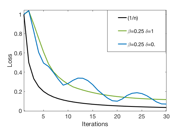
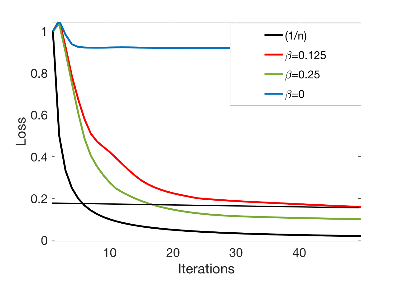
Figure 1: Synthetic dataset. Left convergence of Algorithm 2 shows the benefit of using "Huber" function instead of $\ell_{1}$ loss (i.e. $\delta=0$). Right: This figure shows the benefit of the augmented variable $\mu$ for improving convergence.

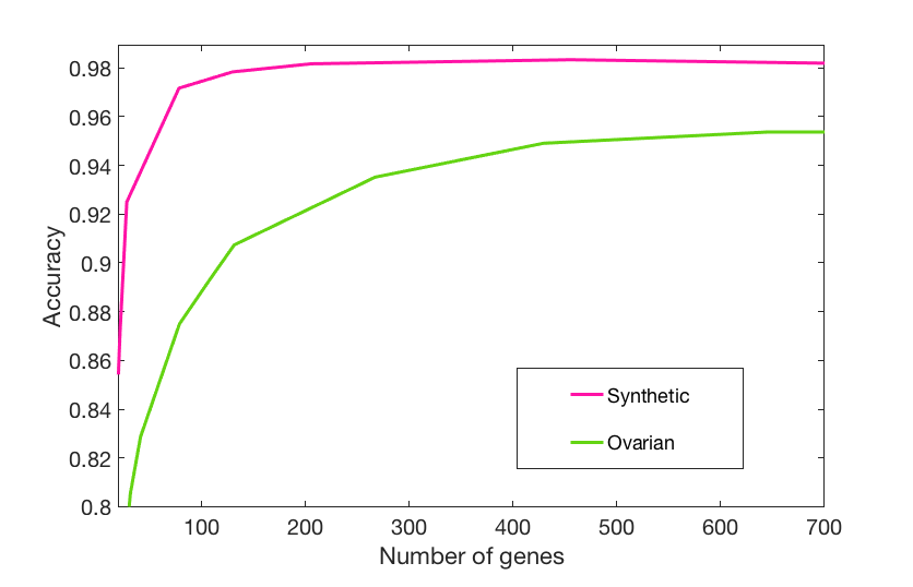
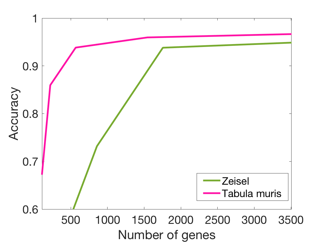
Figure 2: Left: Synthetic and Ovarian dataset; Right Tabula Muris dataset and Zeisel dataset: This plots show a break in the slope of the accuracy curve versus the number of selected genes; this drastic change can be easily detected and used to determine the relevant (and small) number of genes to be used for the analysis.

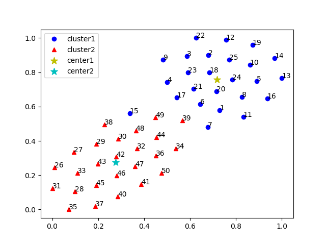
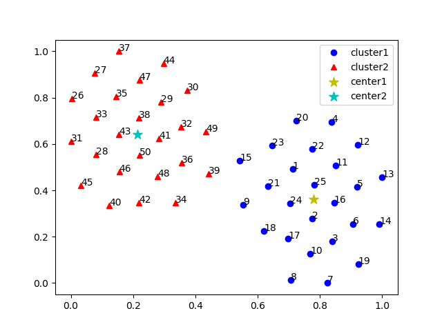
Figure 3: Tsne Van der Maaten and Hinton (2008) of the projected data using constraint $\mu=I$ (left) and estimated $\mu$ (right)on Thyroid dataset

.

Methods	Primal-dual $\mu$	Primal-dual $\mu=I$
Ovarian	94.4%	82.4%
Thyroid	92%	70%
Zeisel	93.07%	93.04%
Tabula	97.9%	97.3%

Table 1: Accuracy test: This table shows that accuracy using primal-dual using estimated $\mu$ outperforms primal-dual using $\mu=I$ both on Ovarian and Thyroid datasets

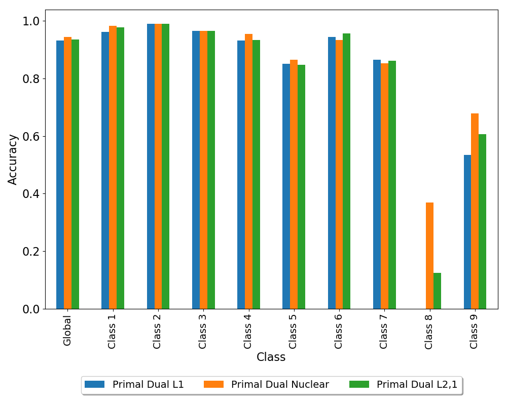
Figure 4: Global accuracy and accuracy in each class: Comparison of $\ell_{1}$, $\ell_{2,1}$ constraint and Nuclear constraint on Zeisel dataset

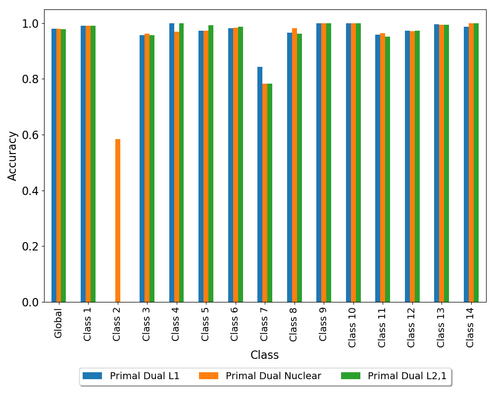
Figure 5: Global accuracy and accuracy in each class: Comparison of $\ell_{1}$, $\ell_{2,1}$ constraint and Nuclear constraint on Tabula Muris dataset

4.3 Accuracy, signature

Figure 1 shows the convergence of the $\ell_{1}$ loss and Huber loss in the training set (normalized by the value of the first iterate). Note an oscillatory convergence of the $\ell_{1}$ loss while convergence of Huber loss is perfectly smooth. Fig. 3 and Table. 1, show the improvement when using adaptive $\mu$ instead of $\mu=I$ for small values of $k$. Our primal-dual algorithm provides accuracy for each cluster. Fig. 4 and Fig. 5, illustrating the reliability of the signature: Nuclear norm constraint and $\ell_{2,1}$ constraint improve accuracy small classes. Note that the standard linear regression approach does not provide accuracy. Moreover Fig. 2 shows a break in the slope of accuracy curve versus the number of selected genes; this drastic change of slope can be easily detected and used to determine the relevant (and small) number of genes to be used for the analysis.

4.4 Complexity and scalability

Table(2) shows that complexity of our primal-dual algorithm is $O(d\times m)$ for primal iterates and $O(m\times k)$ for dual iterates. Note that FISTA requires that one part of the objective is smooth and the other can be easily solved implicitly. This would be the case for instance, for a problem of the form :

$$\min_{W,\mu}\|Y\mu-XW\|_{F}^{2}+\frac{\rho}{2}\|I_{k}-\mu\|_{F}^{2}+\lambda\|W\|_{1}$$ (18)

With the first squared Frobenius norm replaced with a 1 norm, this structure is lost (also in the dual, as the objective is strongly convex only in $\mu$) and there is no way to implement an accelerated method (while a subgradient method would be more expensive). The only reasonable alternative would be ADMM, which makes sense as long as the matrix inversions are not too hard to tackle (here it would be very computationally expensive when $m$ and > $d$ are large and matrix X full rank). Table 2 shows that the primal-dual method outperforms ADMM for high dimensional dataset.

Table 2: Complexity of algorithms primal-dual versus ADMM (X matrix size is $m\times d,$ with m=1000). Time in milliseconds

d	500	$1000$	2000	4000	8000	16000
Primal-dual	20	60	170	397	784	1620
ADMM	117	706	4,630	32,700	-	-

We evaluate the complexity of the different constraint projections using random matrices of size $d\times k$ with $k=10$.

Table 3: Complexity of projections ($W$ size is $d\times k,$ with $k=10$ ). Time in milliseconds

d	$\ell_{1}$	$\ell_{2,1}$	Nuclear	$\ell_{1,2}$
1000	0.75	0.13	0.46	1.91
2000	1.55	0.51	0.48	5.1
4000	3.12	0.91	0.89	12
8000	6.26	1.82	1.6	24
16000	13.8	4.01	3.35	54

We evaluate the complexity of the different constraint projections using random matrices of size $d\times k$ with $d=1000$.

Table 4: Complexity of projections ($W$ size is $d\times k,$ with $d=1000$). Time in milliseconds

k	$\ell_{1}$	$\ell_{2,1}$	Nuclear	$\ell_{1,2}$
10	0.75	0.13	0.46	1.91
50	3.72	0.31	2.23	5.3
100	7.8	0.58	5.01	10.04
200	16.3	1.18	12.3	19
500	47.7	6.44	59.6	55.3
1000	99	16.8	202	110

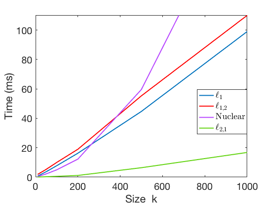
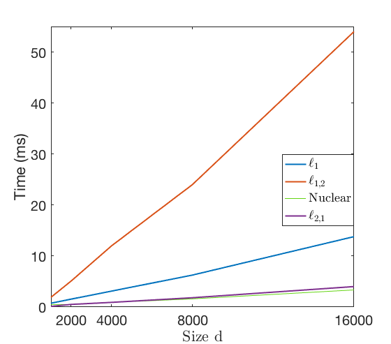
Figure 6: This figure shows left: time as function of size k for d =1000; right : time as function of d for k=10 for different projections.

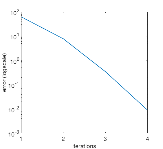
Figure 7: This figure shows the fast convergence of Newton method (logscale).

The cost of the projection on the $\ell_{1}$ ball is expected to be $O(d\times\ k\log(d\times\ k)$. The cost of the projection on the $\ell_{2,1}$ ball is $O(d\times\ k+d\times\ log(d))$ and thus faster than projection on the $\ell_{1}$ ball. Table. 4 and Fig(6) show that for small $k$ the projection cost on the nuclear constraint is similar to projection cost on the $\ell_{2,1}$ ball; however, for large $k$ the projection on the nuclear constraint is not scalable. Fig(6) shows that the cost of the projection on the $\ell_{1,2}$ ball is linear with d and k and slightly greater than the projection on the $\ell_{1}$ ball. Note that the complexity of the projection on the constraint (Table. 4) is lower than the complexity of the algorithm (Table. 2). Thus our constrained Primal-dual method is scalable.

Table 5: Real datasets. Time in milliseconds/iteration for Primal-dual

Dataset	Primal dual	$\ell_{1}$ Projection
Synthetic m=600 , d=15,000	16	6.1
Ovarian m=216 , d=15,000	6.33	6.1
Zeisel m=3005 , d=7,364	36.6	13.7
Tabula m=5400 , d=10,516	110	28.8

5 Discussion

The goal of our paper is to provide sparse and robust features for each class. However the number of features (the sparsity) is a key issue. In order to cope with it, we propose to use accuracy in a k-fold cross validation procedure. To do so, we define $\ell_{1}$ centers $\mu_{j}$ as minimizers of the $\ell_{1}$ distortion in class $j$ instead of using standard centroids. With $\mu$ being the matrix of centers and Y the matrix of known labels (supervised classification), the norm of the matrix $Y\mu-XW$ is the sum of the distortions over all the classes. The main benefits of this $\mu$ modeling is illustrated on Ovarian and Thyroid dataset. We emphasize two important features of our method: (i) contrary to standard approaches based on $\ell_{1}$ constraints, it provides a structured signature adapted to each class; (ii) it also provides a small number of features (sparsity) for efficient classification. Another original point of our algorithm is that we optimize simultaneously over the centers $\mu$ and over the matrix of weights W employed for projection. The complexity of our algorithm is linear with both variables $m$ and $d$. Although it is not easy to carry out a fair comparison among the different methods, due to the issue of implementation or the choice of parameters, we propose the following complexity comparison. ADMM is also reference method for tackling this problem. However, ADMM requires (large) matrix inversions and is hard to implement when these are not structured. ADMM is computationally expensive when $m$ and $d$ are large and matrix X full rank). Numerical experiments illustrate the benefits of our approach.

6 Conclusion

We have proposed a new primal-dual method for supervised classification based on a robust Huber loss for the data and $\ell_{1}$, nuclear or $\ell_{2,1}$ constraints for feature selection. Our algorithm computes jointly a projection matrix $W$ and a matrix of centers $\mu$ that are used to build a classifier. The algorithm provides a structured signature (and an estimate of its reliability) together with a minimum number of genes. We establish convergence results and show the effectiveness of our method on synthetic and biological data. Extending the method to other criteria is easy on condition that efficient projection (on the dual ball for the loss data term) and $\mathrm{proj}$ (for the regularization term) algorithms are available.

A Regularization with constrained $\ell_{1,2}$ norm

The problem is, given $(v_{i,j})_{i=1,\dots,n}^{j=1,\dots,m}$, to find $w=(w_{i,j})$ which solves

$$\min_{w}\left\{\sum_{i,j}|w_{i,j}-v_{i,j}|^{2}:\sum_{i}\left(\sum_{j}|w_{i,j}|\right)^{2}\leq\eta^{2}\right\}.$$ (19)

The most direct approach is to introduce a Lagrange multiplier for the constraint and then compute it by means of Newton’s method. Let us therefore first consider, for $\lambda>0$:

$$\min_{w}\sum_{i,j}|w_{i,j}-v_{i,j}|^{2}+\lambda\sum_{i}\Big{(}\sum_{j}|w_{i,j}|\Big{)}^{2}.$$ (20)

This has the advantage to decouple into $n$ independent minimization problems as follows:

$$\sum_{i}\min_{w_{i,\cdot}}\sum_{j}|w_{i,j}-v_{i,j}|^{2}+\lambda\Big{(}\sum_{j}|w_{i,j}|\Big{)}^{2}.$$ (21)

We first consider the generic subproblem (dropping the index $i$):

$$\min_{w_{j}}\sum_{j}|w_{j}-v_{j}|^{2}+\lambda\Big{(}\sum_{j}|w_{j}|\Big{)}^{2}$$ (22)

whose solution is easily seen to satisfy:

$$w_{j}=\Big{(}|v_{j}|-\lambda\sum_{j^{\prime}}|w_{j^{\prime}}|\Big{)}^{+}\textup{sgn}v_{j}.$$ (23)

Hence, letting $\delta=\lambda\sum|w_{j}|$, one sees that one needs to find $\delta$ such that

$$\delta=\lambda\sum_{j}(|v_{j}|-\delta)^{+}$$ (24)

which has a unique solution in $[0,\max_{j}|v_{j}|]$. If $|v_{j}|$ are sorted in decreasing order, one must find $p\in\{1,\dots,m\}$ such that if

$$\delta=\frac{\lambda\sum_{j=1}^{p}|v_{j}|}{1+\lambda p}$$ (25)

one has $|v_{p}|\geq\delta$, $|v_{p+1}|\leq\delta$. It means in fact that

$$\delta=\lambda\max_{p\in\{1,\dots,m\}}\frac{\sum_{j=1}^{p}|v_{j}|}{1+\lambda p}$$ (26)

Indeed, one can see the previous expression as the average of $0$ with weight $1/\lambda$ and $|v_{j}|$, $j=1,\dots,p$: $\delta=((1/\lambda)\times 0+\sum_{j=1}^{p}|v_{j}|)/(1/\lambda+p)$ which will increase as long as one adds terms above the average, and then decrease. Observe in addition that

$$\sum_{j}(|v_{j}|-\delta)^{+}=\frac{\delta}{\lambda}=\max_{p\in\{1,\dots,m\}}\frac{\sum_{j=1}^{p}|v_{j}|}{1+\lambda p}.$$ (27)

If we return to our original problem (19), we see that one needs to find $\lambda\geq 0$ such that (assuming all $|v_{i,\cdot}|$ are sorted in decreasing order and defining $S_{i,p}:=\sum_{j=1}^{p}|v_{i,j}|$):

$$\sum_{i=1}^{n}\max_{p_{i}\in\{1,\dots,m\}}\left(\frac{S_{i,p_{i}}}{1+\lambda p_{i}}\right)^{2}=\eta^{2}$$ (28)

This is found by Newton’s method. The function in (28) is convex (as a max of convex functions), decreasing in $\lambda$. Starting from $\lambda^{0}$ and the corresponding values $p_{i}^{0}$, $i=1,\dots,n$ one should compute iteratively:

$$\lambda^{k+1}=\lambda^{k}+\frac{\sum_{i=1}^{n}\left(\frac{S_{i,p_{i}^{k}}}{1+\lambda^{k}p_{i}^{k}}\right)^{2}-\eta^{2}}{2\sum_{i=1}^{n}p_{i}^{k}\frac{(S_{i,p_{i}^{k}})^{2}}{(1+\lambda^{k}p_{i}^{k})^{3}}}$$ (29)

and then update $p_{i}^{k+1}$ by finding for each $i$:

$$\max_{p_{i}\in\{1,\dots,m\}}\frac{S_{i,p_{i}}}{1+\lambda^{k+1}p_{i}}.$$ (30)

This process must converge as the function to invert in (28) is convex and decreasing, in particular if $\lambda^{0}$ is less than the optimal lambda it is easy to see that $(\lambda^{k})$ will converge monotonically, increasing towards the optimal value. It is not difficult to prove that this convergence is at least linear (with rate $1-f^{\prime}(\lambda^{*})/f^{\prime}(\lambda^{0})$ if $f(\lambda)$ denotes the left-hand side of (28) and $\lambda^{*}$ the solution), and it is classical that it becomes quadratic when $\lambda^{k}$ is close enough to the optimum (hence the importance of finding a good starting point). Once this has converged, one gets the thresholds $\delta_{i}$ by the formula

$$\delta_{i}=\lambda^{k}\frac{S_{i,p_{i}^{k}}}{1+\lambda^{k}{p_{i}^{k}}}$$ (31)

and then $w_{i,j}=(|v_{i,j}|-\delta_{i})^{+}\textup{sgn}v_{i,j}$ can be easily computed on the unsorted data.

Initial $\lambda$:

the process will converge faster is one can find a good estimate of the optimal $\lambda$ as an initial guess. One has for the optimal $\lambda^{*}$:

$$\max_{\vec{p}=(p_{1},\dots,p_{n})}\sum_{i}\frac{S_{i,p_{i}}^{2}}{(1+\lambda^{*}p_{i})^{2}}=\eta^{2}\geq\max_{p\in\{1,\dots,m\}}\frac{\sum_{i}S_{i,p}^{2}}{(1+\lambda^{*}p)^{2}}.$$

The idea here is that the max on arbitrary vectors $(p_{1},\dots,p_{n})$ is replaced with a (smaller) max over vectors $(p,p,\dots,p)$ with identical coordinates. It follows easily that:

$$\lambda^{*}\geq\max_{p\in\{1,\dots,m\}}\frac{\frac{1}{\eta}\sqrt{\sum_{i}S_{i,p}^{2}}-1}{p}\cdot$$ (32)

In practice, we take the right-hand side of (32) as initial $\lambda^{0}$.

B Extension to other criteria: Frobenius loss minimization

Our method can be extended straightforwardly to other criteria provided that we can compute the projection on the dual ball for the loss data term. In this paper, we study an algorithm for the Frobenius norm. Note that our approach based on a dual computation of the norm allows us to use the norm itself, instead of the squared Frobenius norm.

We consider the following criterion:

$$\min_{(W,\mu)}\|Y\mu-XW\|_{F}+\frac{\rho}{2}\|I_{k}-\mu\|_{F}^{2}\text{ s.t. }\quad\|W\|_{1}\leqslant\eta,$$ (33)

and dualize according to

$$\min_{(W,\mu)}\max_{\|Z\|_{F}\leqslant 1}\!\!\langle Z,Y\mu-XW\rangle+\frac{\rho}{2}\|I_{k}-\mu\|^{2}_{F}\text{ s.t. }\|W\|_{1}\leqslant\eta.$$ (34)

Obvious modifications of the previous scheme lead to Algorithm:

1:  Input: $X,Y,N,\sigma,\tau,\eta,\delta,\rho,\mu_{0},W_{0},Z_{0}$

2:  $W:=W_{0}$

3:  $\mu:=\mu_{0}$

4:  $Z:=Z_{0}$

5:  for $n=1,\dots,N$ do

6:     $W_{\text{old}}:=W$

7:     $\mu_{\text{old}}:=\mu$

8:     $W:=W+\tau\cdot(X^{T}Z)$

9:     $W:=\mathrm{proj}(W,\eta)$

10:     $\mu:=\frac{1}{1+\tau_{\mu}\cdot\rho}(\mu_{\text{old}}+\rho\cdot\tau_{\mu}I_{k}-\tau_{\mu}\cdot(Y^{T}Z))$

11:     $Z:=Z+\sigma\cdot(Y(2\mu-\mu_{\text{old}})-X(2W-W_{\text{old}}))$

12:     $Z:=Z/\max\{1,\|Z\|_{F}\})$

13:  end for

14:  Output: $W,\mu$

Algorithm 6 Primal-dual algorithm for Frobenius loss minimization: constrained case.

C Accelerated Constrained primal-dual approach

By using strong convexity with respect to Z Chambolle and Pock (2011), we can accelerate the dual primal algorithm as follows:

$$Z^{n+1}:=\mathrm{proj}_{\{|Z_{ij}|\leq 1\}}\left(\frac{Z+\sigma(Y\mu^{n}-XW^{n})}{1+\sigma\delta}\right)$$

$$\theta:=\frac{1}{\sqrt{1+\delta\sigma}},\quad\bar{Z}:=Z^{n+1}+\theta(Z^{n+1}-Z^{n});$$

$$\sigma=\sigma*\theta;\quad\tau=\frac{\tau}{\theta};\quad\tau_{\mu}=\frac{\tau_{\mu}}{\theta};$$

$$W^{n+1}:=\arg\min_{\|W\|_{1}\leq\eta}\frac{1}{2\tau}\|W-W^{n}\|^{2}_{F}-\langle X^{T}\bar{Z},W\rangle$$

$$\mu^{n+1}:=\dfrac{1}{1+\tau_{\mu}\rho}(\mu^{n}+\rho\tau_{\mu}I_{k}-\tau_{\mu}Y^{T}\bar{Z})$$

1:  Input: $X,Y,N,\sigma,\tau,\eta,\delta,\rho,\mu_{0},W_{0},Z_{0}$

2:  $W:=W_{0}$

3:  $\mu:=\mu_{0}$

4:  $Z:=Z_{0}$

5:  for $n=1,\dots,N$ do

6:     $W_{\text{old}}:=W$

7:     $\mu_{\text{old}}:=\mu$

8:     $Z_{\text{old}}:=Z$

9:     $W:=W+\tau\cdot(X^{T}Z)$

10:     $W:=\mathrm{proj}(W,\eta)$

11:     $\mu:=\frac{1}{1+\tau_{\mu}\cdot\rho}(\mu_{\text{old}}+\rho\cdot\tau_{\mu}I_{k}-\tau_{\mu}\cdot(Y^{T}Z))$

12:     $Z:=\frac{1}{1+\sigma\cdot\delta}(Z+\sigma\cdot(Y(2\mu-\mu_{\text{old}})-X(2W-W_{\text{old}})))$)

13:     $Z:=\max(-1,\min(1,Z))$)

14:     $\theta:=\frac{1}{\sqrt{1+\delta\sigma}};\quad Z:=Z+\theta(Z-Z_{\text{old}});$$\sigma=\sigma*\theta;\quad\tau=\frac{\tau}{\theta};\quad\tau_{\mu}=\frac{\tau_{\mu}}{\theta}$

15:  end for

16:  Output: $W,\mu$

Algorithm 7 Primal-dual algorithm, accelerated constrained case—$\mathrm{proj}(V,\eta)$ is the projection on the $\ell_{1}$ ball of radius $\eta$ (see Condat (2016)).

An over-relaxed variant of the previous algorithm is presented below (Algorithm 8).

1:  Input: $X,Y,N,\sigma,\tau,\tau_{\mu},\eta,\delta,\rho,\mu_{0},W_{0},Z_{0},\gamma\in(-1,1)$

2:  for $n=1,\dots,N$ do

3:     $W_{\text{old}}:=W$

4:     $\mu_{\text{old}}:=\mu$

5:     $W:=W+\tau\cdot(X^{T}Z)$

6:     $W:=\mathrm{proj}(W,\eta)$

7:     $\mu:=\frac{1}{1+\tau_{\mu}\rho}(\mu+\rho\tau_{\mu}I_{k}-\tau_{\mu}(Y^{T}Z))$

8:     $Z:=\frac{1}{1+\sigma\cdot\delta}\cdot(Z+\sigma\cdot(Y(2\mu-\mu_{\text{old}})-X(2W-W_{\text{old}})))$

9:     $Z:=\max(-1,\min(1,Z))$)

10:     $W:=W+\gamma(W-W_{\text{old}})$

11:     $\mu:=\mu+\gamma(\mu-\mu_{\text{old}})$

12:     $Z:=Z+\gamma(Z-Z_{\text{old}})$

13:  end for

14:  Output: $W,\mu$

Algorithm 8 Primal-dual algorithm, constrained case with over-relaxation.

The convergence condition discussed in Appendix E imposes that

$$\boxed{\sigma\left(\tau_{\mu}\|Y\|^{2}+\tau\|X\|^{2}\right)<1},$$ (35)

D Regularization with constrained elastic net

In order to handle features with high correlation, We consider the convex constrained supervised classification problem,

$$\min_{(W,\mu)}\|Y\mu-XW\|_{1}+\frac{\rho}{2}\|I_{k}-\mu\|_{F}^{2}+\frac{\alpha}{2}\|W\|_{F}^{2}\text{ s.t. }\quad\|W\|_{1}\leqslant\eta,$$ (36)

that we dualize as before:

$$\min_{(W,\mu)}\max_{\|Z\|_{\infty}\leqslant 1}\!\!\langle Z,Y\mu-XW\rangle+\frac{\rho}{2}\|I_{k}-\mu\|_{F}^{2}+\frac{\alpha}{2}\|W\|_{F}^{2}\text{ s.t. }\|W\|_{1}\leqslant\eta.$$ (37)

We adapt the update of $W$ of Algorithm 1 by using a shrinkage on $W$, and devise Algorithm 9.

1:  Input: $X,Y,N,\sigma,\tau,\eta,\delta,\alpha,\rho,\mu_{0},W_{0},Z_{0}$

2:  $W:=W_{0}$

3:  $\mu:=\mu_{0}$

4:  $Z:=Z_{0}$

5:  for $n=1,\dots,N$ do

6:     $W_{\text{old}}:=W$

7:     $\mu_{\text{old}}:=\mu$

8:     $W:=\frac{1}{1+\tau\alpha}(W+\tau(X^{T}Z))$

9:     $W:=\mathrm{proj}(W,\eta)$

10:     $\mu:=\frac{1}{1+\tau_{\mu}\cdot\rho}(\mu_{\text{old}}+\rho\cdot\tau_{\mu}I_{k}-\tau_{\mu}\cdot(Y^{T}Z))$

11:     $Z:=\frac{1}{1+\sigma\cdot\delta}(Z+\sigma\cdot(Y(2\mu-\mu_{\text{old}})-X(2W-W_{\text{old}})))$)

12:     $Z:=\max(-1,\min(1,Z))$

13:  end for

14:  Output: $W,\mu$

Algorithm 9 Primal-dual algorithm, with elastic net constrained case.

E Convergence Analysis

E.1 Convergence of primal-dual algorithms

The proof of convergence of the algorithms relies on Theorems 1 and 2 in Chambolle and Pock (2016) which we slightly adapt for our setting. The algorithms we present here correspond to Alg. 1 and 2 in that reference, adapted to the particular case of problem (5) and its saddle-point formulation (11). In addition, here, the primal part of the objective is “partially strongly convex” ($\rho$-strongly convex with respect to the variable $\mu$, thanks to the term $(\rho/2)\|\mu-I\|^{2}$. (We could exploit this to gain “partial acceleration” Valkonen and Pock (2017), however at the expense of a much more complex method and no clear gain for the variable $W$, while translated in the Euclidean setting, Chambolle and Pock (2016) remains simple and easy to improve.) For our setting we consider a general objective of the form:

$$\min_{x,x^{\prime}}\max_{y}f(x)+g(x^{\prime})+\langle{Kx+K^{\prime}x^{\prime}},{y}\rangle-h^{*}(y)$$ (38)

for $f,g,h$ convex functions whose “prox” (see below) are easy to compute and $K,K^{\prime}$ linear operators, and we assume moreover $f$ is $\rho$-strongly convex for some $\rho>0$. We will show how this last property can be exploited to “boost” the convergence, allowing for larger steps than usually suggested by other authors. When computing the “prox” $\hat{x}$ at point $\bar{x}$ of a $\rho$-strongly convex function $x\mapsto f(x)$, with parameter $\tau$, that is, the minimizer

$$\hat{x}=\mathrm{prox}_{\tau f}(\bar{x}):=\arg\min_{x}f(x)+\frac{\|x-\bar{x}\|^{2}}{2\tau},$$ (39)

one has for all test point $x$:

$$f(x)+\frac{\|x-\bar{x}\|^{2}}{2\tau}\geq f(\hat{x})+\frac{\|\hat{x}-\bar{x}\|^{2}}{2\tau}+\frac{\|x-\hat{x}\|^{2}}{2\tau}+\frac{\rho}{2}\|x-\hat{x}\|^{2}.$$ (40)

However, combined with non-strongly convex iterates, the slight improvement given by the factor $\rho$ is hard to exploit (whereas for simple gradient descent type iterates one obviously can derive linear convergence to the optimum), see for instance Valkonen and Pock (2017) for a possible strategy. We exploit here this improvement in a different way. We combine the parallelogram identity

$$\|x-\bar{x}\|^{2}+\|x-\hat{x}\|^{2}=\frac{1}{2}\|\bar{x}-\hat{x}\|^{2}+2\left\|x-\tfrac{\bar{x}+\hat{x}}{2}\right\|^{2}$$

with the previous inequality to obtain:

$$f(x)+(1+\tau\tfrac{\rho}{2})\frac{\|x-\bar{x}\|^{2}}{2\tau}\geq f(\hat{x})+(1+\tau\tfrac{\rho}{4})\frac{\|\hat{x}-\bar{x}\|^{2}}{2\tau}+(1+\tau\tfrac{\rho}{2})\frac{\|x-\hat{x}\|^{2}}{2\tau}.$$ (41)

The first type of algorithm we consider is Algorithm LABEL:algo1, which corresponds to Alg. 1 in Chambolle and Pock (2016) (see also Pock et al. (2009); Esser et al. (2010); Chambolle and Pock (2011)). It consists in tackling problem (38) by alternating a proximal descent step in $x,x^{\prime}$ followed by an ascent step in $y$:

$$\begin{split}x^{n+1}&=\mathrm{prox}_{\tau f}(x^{n}-\tau K^{T}y^{n}),\\ {x^{\prime}}^{n+1}&=\mathrm{prox}_{\tau^{\prime}g}({x^{\prime}}^{n}-\tau^{\prime}{K^{\prime}}^{T}y^{n}),\\ y^{n+1}&=\mathrm{prox}_{\sigma h^{*}}(y^{n}+\\ &\sigma(K(2x^{n+1}-x^{n})+K^{\prime}(2{x^{\prime}}^{n+1}-{x^{\prime}}^{n}))).\end{split}$$ (42)

We then introduce the “ergodic” averages

$$X^{N}=\tfrac{1}{N}\sum_{n=1}^{N}x^{n},\ {X^{\prime}}^{N}=\tfrac{1}{N}\sum_{n=1}^{N}{x^{\prime}}^{n},\ Y^{N}=\tfrac{1}{N}\sum_{n=1}^{N}y^{n}.$$

Theorem 1 in Chambolle and Pock (2016), shows with an elementary proof the estimate, for any test point $(x,x^{\prime},y)$:

$$\mathcal{L}(X^{N},{X^{\prime}}^{N},y)-\mathcal{L}(x,x^{\prime},Y^{N})\leq\frac{1}{2N}\left\|\begin{pmatrix}x\\ x^{\prime}\\ y\end{pmatrix}-\begin{pmatrix}x^{0}\\ {x^{\prime}}^{0}\\ y^{0}\end{pmatrix}\right\|^{2}_{M_{\tau,\tau^{\prime},\sigma}}$$ (43)

where $\mathcal{L}$ is the Lagrangian function in (38) and provided the matrix $M_{\tau,\tau^{\prime},\sigma}$, given by

$$M_{\tau,\tau^{\prime},\sigma}=\begin{pmatrix}\frac{I}{\tau}&0&-K^{T}\\ 0&\frac{I}{\tau^{\prime}}&-{K^{\prime}}^{T}\\ -K&-K^{\prime}&\frac{I}{\sigma}\end{pmatrix}$$ (44)

is positive-definite. Before exploiting the estimate (43), let us express the conditions on $\tau,\tau^{\prime},\sigma$ which ensure that this is true. We need that for any $(\xi,\xi^{\prime},\eta)\neq 0$,

$$\frac{1}{\tau}\|\xi\|^{2}+\frac{1}{\tau^{\prime}}\|\xi^{\prime}\|^{2}+\frac{1}{\sigma}\|\eta^{2}\|>2\langle{K\xi},{\eta}\rangle+2\langle{K^{\prime}\xi^{\prime}},{\eta}\rangle$$

and obviously, this is the same as requiring that for any $a,a^{\prime},b$ positive numbers,

$$\frac{a^{2}}{\tau}+\frac{a^{\prime 2}}{\tau^{\prime}}+\frac{b^{2}}{\sigma}>2(\|K\|a+2\|K^{\prime}\|a^{\prime})b.$$

The worst $b$ in this inequality is $b=\sigma(\|K\|a+2\|K^{\prime}\|a^{\prime})$, then one checks easily that the worse $a,a^{\prime}$ are of the form $\bar{a}\|K\|\tau$, $\bar{a}\|K^{\prime}\|\tau^{\prime}$ respectively, so that one should have for all $\bar{a}\neq 0$:

$$\bar{a}^{2}\left(\|K\|^{2}\tau+\|K^{\prime}\|^{2}\tau^{\prime}\right)>\sigma\bar{a}^{2}\left(\|K\|^{2}\tau+\|K^{\prime}\|^{2}\tau^{\prime}\right)^{2},$$

yielding the condition

$$\sigma(\tau\|K\|^{2}+\tau^{\prime}\|K^{\prime}\|^{2})<1.$$

We notice in addition that under such a condition, one also has

$$M_{\tau,\tau^{\prime},\sigma}\leq 2\begin{pmatrix}\frac{I}{\tau}&&\\ &\frac{I}{\tau^{\prime}}&\\ &&\frac{I}{\sigma}\end{pmatrix}$$

which allows to simplify a bit the expression in the right-hand side of (43) (at the expense of a factor $2$ in front of the estimate).

We have not made use of the strong convexity up to now, and in particular, of (41). A quick look at the proof of Theorem 1 in Chambolle and Pock (2016) shows that it will improve slightly the latter condition, allowing to replace $\tau$ with the smaller effective step $\tau/(1+\tau\rho/4)$, yielding the new condition

$$\sigma\left(\frac{\tau}{1+\tau\frac{\rho}{4}}\|K\|^{2}+\tau^{\prime}\|K^{\prime}\|^{2}\right)<1.$$ (45)

This ensures now that (43) holds with $M_{\tau,\tau^{\prime},\sigma}$ replaced with

$$M_{\tau,\tau^{\prime},\sigma,\rho}=\begin{pmatrix}\left(\frac{1}{\tau}+\frac{\rho}{2}\right)I&0&-K^{T}0&\frac{I}{\tau^{\prime}}&-{K^{\prime}}^{T}\\ -K&-K^{\prime}&\frac{I}{\sigma}\end{pmatrix}\leq\begin{pmatrix}\left(\frac{2}{\tau}+\frac{3\rho}{4}\right)I&0&0\\ 0&\frac{2}{\tau^{\prime}}I&0\\ 0&0&\frac{2}{\sigma}I\end{pmatrix}$$ (46)

where the last inequality follows from (45). Applied to problem (11), which is $\rho$-convex in $\mu$, we find that (45) becomes the condition

$$\boxed{\sigma\left(\frac{\tau_{\mu}}{1+\tau_{\mu}\frac{\rho}{4}}\|Y\|^{2}+\tau\|X\|^{2}\right)<1.}$$ (47)

When (47) holds, then the ergodic iterates (here we denote $W^{n}$, etc, the value of $W$ computed at the end of iteration $n$):

$$\bar{W}^{N}=\frac{1}{N}\sum_{n=1}^{N}W^{n},\ {\bar{\mu}}^{N}=\frac{1}{N}\sum_{n=1}^{N}{\mu}^{n},\ \bar{Z}^{N}=\frac{1}{N}\sum_{n=1}^{N}Z^{n}.$$ (48)

satisfy for all $W,\mu,Z$:

$$\mathcal{L}(\bar{W}^{N},\bar{\mu}^{N},Z)-\mathcal{L}(W,\mu,\bar{Z}^{N})\leq\frac{1}{N}\Big{(}\frac{3\rho}{8}\|\mu-\mu^{0}\|^{2}+\frac{\|\mu-\mu^{0}\|^{2}}{\tau_{\mu}}+\frac{\|W-W^{0}\|^{2}}{\tau}+\frac{\|Z-Z^{0}\|^{2}}{\sigma}\Big{)}.$$ (49)

Here the Lagrangian $\mathcal{L}$ is:

$$\mathcal{L}(W,\mu,Z)=\langle{Z},{Y\mu-XW}\rangle+\lambda\|W\|_{1}+\frac{\rho}{2}\|I-\mu\|^{2}.$$

We denote $\mathcal{E}(W,\mu)=\sup_{Z}\mathcal{L}(W,\mu,Z)$ the primal energy (which appears in (5)) and remark that in (11), $Z$ is bounded ($|Z_{i,j}|\leq 1$ for all $i,j$) so that $\|Z-Z^{0}\|^{2}\leq 4mk$ in (49). Hence, taking the supremum on $Z$ and choosing for $(W,\mu)$ a primal solution (minimizer of $E$) $(W^{*},\mu^{*})$, we deduce:

$$\mathcal{E}(\bar{W}^{N},\bar{\mu}^{N})-\mathcal{E}(W^{*},\mu^{*})\leq\frac{1}{N}\left(\frac{4mk}{\sigma}+\Big{(}\frac{3\rho}{8}+\frac{1}{\tau_{\mu}}\Big{)}\|\mu^{*}-\mu^{0}\|^{2}+\frac{\|W^{*}-W^{0}\|^{2}}{\tau}\right).$$ (50)

In general, if one can compute reasonable estimates $\Delta_{\mu}$, $\Delta_{W}$ for these quantities, one should take:

$$\begin{split}&\tau=\frac{\Delta_{W}}{2\sqrt{mk}\|X\|},\ \tau_{\mu}=\begin{cases}\frac{1}{\frac{2\sqrt{mk}\|Y\|}{\Delta_{\mu}}-\frac{\rho}{4}}&\textup{ if }\frac{8\sqrt{mk}\|Y\|}{\rho\Delta_{\mu}}>1\\ \tau_{\mu}>>1&\textup{ else,}\end{cases}\\ &\sigma=\frac{1}{\frac{\tau_{\mu}}{1+\tau_{\mu}\frac{\rho}{4}}\|Y\|^{2}+\tau\|X\|^{2}}.\end{split}$$

to obtain (considering here only the case $\rho$ small, that is when $\rho\Delta_{\mu}\leq 8\sqrt{mk}\|Y\|$):

$$\mathcal{E}(\bar{W}^{N},\bar{\mu}^{N})-\mathcal{E}(W^{*},\mu^{*})\leq\frac{\sqrt{mk}(5\Delta_{\mu}\|Y\|+4\Delta_{W}\|X\|)}{N},$$ (51)

There is no clear way how to estimate a priori the norm $\|W^{*}-W^{0}\|$ in the Lagrangian approach.

Remark 1

Note that for the $\ell_{1}$ constrained problem (7) $\Delta_{W}$ is bounded. Since $\|W\|_{1}\leq\eta$: $\|W^{*}-W^{0}\|\leq\|W^{*}-W^{0}\|_{1}\leq 2\eta$, we use the estimate $\Delta_{W}\leq 2\eta$. Using the initial value $\mu^{0}=I_{k}$, $\Delta_{\mu}$ is also easily shown to be bounded (as $W$ is). Empirically, we found that we can use the estimate $\Delta_{\mu}\lesssim\beta\|I_{k}\|_{F}=\beta\sqrt{k}$ where $\beta$ is a parameter to be tuned. Thus $\rho$ being small we have $\frac{8\sqrt{m}\|Y\|}{\rho\beta}>1$. Moreover, using $\|X\|=1$ ($X$ can be normalized), we obtain the following reasonable choice of parameters:

$$\begin{split}&\tau=\frac{\Delta_{W}}{2\sqrt{mk}}\,,\quad\tau_{\mu}=\frac{\beta}{2\sqrt{m}\|Y\|-(1/4)\beta\rho}\,\\ &\sigma=\frac{1}{\frac{\tau_{\mu}}{1+\tau_{\mu}\frac{\rho}{4}}\|Y\|^{2}+\tau}\cdot\end{split}$$ (52)

In the case of Problem (34) (Sec. B), $Z$ is also bounded but then, one has simply $\|Z^{*}-Z^{0}\|^{2}\leq 4$, hence (50) must be replaced with

$$\mathcal{E}(\bar{W}^{N},\mu^{N})-\mathcal{E}(W^{*},\mu^{*})\leq\frac{1}{N}\left(\frac{4}{\sigma}+\Big{(}\frac{3\rho}{8}+\frac{1}{\tau_{\mu}}\Big{)}\|\mu^{*}-\mu^{0}\|^{2}+\frac{\|W^{*}-W^{0}\|^{2}}{\tau}\right).$$ (53)

(Obviously, now, the energy $\mathcal{E}$ is the primal energy in (33).) The same analysis as before remains valid, but now with $mk$ replaced with $1$.

E.2 Convergence with over-relaxation

For the over-relaxed variant (Algorithm 8), the adaption is a little bit more complicated, and one does not benefit much from taking into account the partial strong convexity. One approach is to rewrite the improved descent rule (41) as follows:

$$f(\hat{x})\leq f(x)+\frac{1+\tau\rho/2}{2\tau}\big{(}\|x-\bar{x}\|^{2}-\|x-\hat{x}\|^{2}\\ -\|\hat{x}-\bar{x}\|^{2}\big{)}+\frac{\rho}{8}\|\hat{x}-\bar{x}\|^{2}\\ =f(x)+\frac{1}{2\widetilde{\tau}}\langle{x-\hat{x}},{\hat{x}-\bar{x}}\rangle+\frac{\rho}{8}\|\hat{x}-\bar{x}\|^{2}$$ (54)

where $\widetilde{\tau}=\tau/(1+\tau\rho/2)$ is an effective time-step. As a result, we observe that the first (primal) update in (42) yields the same rule as an explicit-implicit primal update of a nonsmooth$+$smooth functions with effective step $\widetilde{\tau}$ and Lipschitz constant $\rho/4$, cf Eq. (9) in Chambolle and Pock (2016). Hence, the analysis of these authors (see Sec. 4.1 in the above reference) can be reproduced almost identically and will yield for the over-relaxed algorithm (8) similar convergence rates, cf. (43)-(50), now, with the factor $1/N$ replaced with $1/((1+\gamma)N)$. It requires that the matrix

$$\widetilde{M}=\begin{pmatrix}(\frac{1}{\widetilde{\tau}}-\frac{\rho/4}{1-\gamma})I&0&-K^{T}\\ 0&\frac{I}{\tau^{\prime}}&-{K^{\prime}}^{T}\\ -K^{\prime}&-K&\frac{I}{\sigma}\end{pmatrix}$$ (55)

be positive definite. Observe however that the estimates hold for the ergodic averages (cf (48)) of the variables obtained at the end of Step 12 of Algorithm 8 and Step LABEL:statefinal2 of Algorithm LABEL:PD-L2-OR, rather than for the over-relaxed variables (which could not even be feasible). We derive that for this method, condition (47) should be replaced with

$$\sigma\left(\frac{\tau_{\mu}}{1+\frac{\tau_{\mu}\rho}{4}\frac{1-2\gamma}{1-\gamma}}\|Y\|^{2}+\tau\|X\|^{2}\right)<1,$$ (56)

at least if $\gamma<1/2$.

As seen, for $\gamma\geq 1/2$, the condition obtained for $\rho=0$ is better (hence, the partial strong convexity does not seem to yield any reasonable improvement for this algorithm). It simply reads

$$\sigma\left(\tau_{\mu}\|Y\|^{2}+\tau\|X\|^{2}\right)<1,$$ (57)

and one gets the estimate from Chambolle and Pock (2016) (Eq. (24), further simplified thanks to (56)):

$$\mathcal{E}(\bar{W}^{N},\bar{\mu}^{N})-\mathcal{E}(W^{*},\mu^{*})\leq\frac{1}{(1+\gamma)N}\left(\frac{4mk}{\sigma}+\frac{\|\mu^{*}-\mu^{0}\|^{2}}{\tau_{\mu}}+\frac{\|W^{*}-W^{0}\|^{2}}{\tau}\right).$$ (58)

F Derivation of the min-max iteration

As explained in Section E.1, we consider the following general min-max problem:

$$\min_{(x,x^{\prime})}\max_{y}f(x)+g(x^{\prime})+\langle{Kx+K^{\prime}x^{\prime}},{y}\rangle-h^{*}(y)$$ (59)

for convex functions $f$, $g$, $h$, and linear operators $K$, $K^{\prime}$. Note that, since $h^{*}$ is the convex conjugate of $h$, for any fixed $x^{\prime}$ one has

$$\max_{y}\langle{Kx+K^{\prime}x^{\prime}},{y}\rangle-h^{*}(y)=h^{**}(Kx+K^{\prime}x^{\prime})=h(Kx+K^{\prime}x^{\prime}),$$

so that the problem can also be rewritten as

$$\min_{(x,x^{\prime})}f(x)+g(x^{\prime})+h(Kx+K^{\prime}x^{\prime}).$$

In our situation, we dualize the computation of the $\ell_{1}$ norm containing the linear terms according to

$$\|Y\mu-XW\|_{1}=\max_{\|Z\|_{\infty}\leqslant 1}\langle{Z},{Y\mu-XW}\rangle.$$

As a result, the original minimization

$$\min_{(W,\mu)}\|Y\mu-XW\|_{1}+\lambda\|W\|_{1}+\frac{\rho}{2}\|\mu-I\|_{F}^{2}$$

is changed into the min-max problem

$$\min_{(W,\mu)}\max_{Z}\lambda\|W\|_{1}+\frac{\rho}{2}\|\mu-I\|_{F}^{2}+\langle{Z},{Y\mu-XW}\rangle-\delta_{B_{\infty}}(Z)$$

where $\delta_{B_{\infty}}$ denotes the indicator function of the $\ell_{\infty}$ unit ball. This problem fits in our general min-max framework by setting $(x,x^{\prime}):=(W,\mu)$, $y:=Z$, together with

$$f(W):=\lambda\|W\|_{1},\quad g(\mu):=\frac{\rho}{2}\|\mu-I\|_{F}^{2},$$

$$h^{*}(Z):=\delta_{B_{\infty}}(Z),$$

and $Kx+K^{\prime}x^{\prime}=-XW+Y\mu$. (Note that, as the conjugate of a norm is the indicatrix of the unit ball of the dual norm, one indeed has $h(z)=\|z\|_{1}$.) Similarly, when replacing the $\ell_{1}$ norm with the Huber function for the loss term, one has (in Lagrangian form)

$$\min_{(W,\mu)}h_{\delta}(Y\mu-XW)+\lambda\|W\|_{1}+\frac{\rho}{2}\|\mu-I\|_{F}^{2}$$

which is dualized according to (59) where $f$ and $g$ are defined as before, and where one takes $h_{\delta}$ instead of the $\ell_{1}$-norm for $h$. Using the fact that

$$h_{\delta}^{*}(s)=\delta s^{2}/2+\delta_{[-1,1]}(s)$$

and vectorizing the computation, one obtains

$$\min_{(W,\mu)}\max_{\|Z\|_{\infty}\leqslant 1}\langle{Z},{Y\mu-XW}\rangle+\lambda\|W\|_{1}+\frac{\rho}{2}\|\mu-I\|_{F}^{2}-\frac{\delta}{2}\|Z\|_{F}^{2},$$

from where one retrieves (11).

References

- Argyriou et al. (2008) Andreas Argyriou, Theodoros Evgeniou, and Massimiliano Pontil. Convex multi-task feature learning. Machine Learning, 73(3):243–272, Dec 2008.
- Beck and Teboulle (2009) A. Beck and M. Teboulle. A fast iterative shrinkage-thresholding algorithm for linear inverse problems. SIAM journal on imaging sciences, 2(1):183–202, 2009.
- Boyd et al. (2011) S. Boyd, N. Parikh, E. Chu, B. Peleato, and J. Eckstein. Distributed optimization and statistical learning via the alternating direction method of multipliers. Trends Machine Learning, 3:1–122, 2011.
- Candès et al. (2008) J. Candès, M. B. Wakin, and S. P. Boyd. Enhancing sparsity by reweighted l1 minimization. Journal of Fourier analysis and applications, 2008.
- Chambolle and Pock (2011) A. Chambolle and T. Pock. A first-order primal-dual algorithm for convex problems with applications to imaging. Journal of Mathematical Imaging and Vision, 40(1):120–145, May 2011.
- Chambolle and Pock (2016) Antonin Chambolle and Thomas Pock. On the ergodic convergence rates of a first-order primal-dual algorithm. Math. Program., 159(1-2, Ser. A):253–287, 2016. ISSN 0025-5610.
- Combettes and Pesquet (2011) P. L. Combettes and J.-C. Pesquet. Proximal splitting methods in signal processing. In Fixed-point algorithms for inverse problems in science and engineering, pages 185–212. Springer, 2011.
- Combettes and Wajs (2005) P. L. Combettes and V. R. Wajs. Signal recovery by proximal forward-backward splitting. Multiscale Modeling & Simulation, 4(4):1168–1200, 2005.
- Condat (2016) L. Condat. Fast projection onto the simplex and the l1 ball. Mathematical Programming Series A, 158(1):575–585, 2016.
- Donoho and Elad (2003) D. L. Donoho and M. Elad. Optimally sparse representation in general (nonorthogonal) dictionaries via minimization. Proceedings of the National Academy of Sciences, 100(5):2197–2202, 2003.
- Donoho (2006) D.L Donoho. Compressed sensing. IEEE Trans. Inf. Theor. 52 (4), pages 1289–1306, 2006.
- Duchi et al. (2008) J. Duchi, S. Shalev-Shwartz, Y. Singer, and T. Chandra. Efficient projections onto the l 1-ball for learning in high dimensions. In Proceedings of the 25th international conference on Machine learning, pages 272–279. ACM, 2008.
- Esser et al. (2010) E. Esser, X. Zhang, and T. F. Chan. A general framework for a class of first order primal-dual algorithms for convex optimization in imaging science. SIAM J. Imaging Sci., 3(4):1015–1046, 2010.
- Evanko (2014) D. Evanko. Method of the year 2013: Methods to sequence the dna and rna of single cells are poised to transform many areas of biology and medicine. Nature Methods, Vol 11, 2014.
- Friedman et al. (2010a) J. Friedman, T. Hastie, and R. Tibshirani. Regularization path for generalized linear models via coordinate descent. Journal of Statistical Software, 33:1–122, 2010a.
- Friedman et al. (2010b) Jerome Friedman, Trevor Hastie, and Robert Tibshirani. A note on the group lasso and a sparse group lasso. arXiv preprint arXiv:1001.0736, 2010b.
- Furey et al. (2000) T. S. Furey, N. Cristianini, N. Duffy, D. W. Bednarski, M. Schummer, and D. Haussler. Support vector machine classification and validation of cancer tissue samples using microarray expression data. Bioinformatics, 16(10):906–914, 2000.
- Guyon et al. (2002) I. Guyon, J. Weston, S. Barnhill, and V. Vapnik. Gene selection for cancer classification using support vector machines. Machine learning, 46(1-3):389–422, 2002.
- Guyon et al. (2017) I. Guyon, S. Gunn, M. Nikravesh, and L .) Zadeh. Feature extraction, foundations and applications. studies in fuzziness and soft computing. Physica-Verlag Springer, 2017.
- Hastie et al. (2004) T. Hastie, S. Rosset, R. Tibshirani, and J. Zhu. The entire regularization path for the support vector machine. Journal of Machine Learning Research, 5:1391–1415, 2004.
- Hastie et al. (2015) T. Hastie, R. Tibshirani, and M. Wainwright. Statistcal learning with sparsity: The lasso and generalizations. CRC Press, 2015.
- Jacob et al. (2009) L. Jacob, G. Obozinski, and J.-P. Vert. Group lasso with overlap and graph lasso. In Proceedings of the 26th International Conference on Machine Learning (ICML-09), pages 353–360, 2009.
- Li et al. (2016) Jundong Li, Kewei Cheng, Suhang Wang, Fred Morstatter, Robert P. Trevino, Jiliang Tang, and Huan Liu. Feature selection: A data perspective. ACM Computing Surveys, 50, 2016.
- Lions and Mercier (1979) P.-L. Lions and B. Mercier. Splitting algorithms for the sum of two nonlinear operators. SIAM Journal on Numerical Analysis, 16(6):964–979, 1979.
- (25) Jun Liu and Jieping Ye. Moreau-yosida regularization for grouped tree structure learning. In Advances in Neural Information Processing Systems 23.
- Liu et al. (2009) Jun Liu, Shuiwang Ji, and Jieping Ye. Multi-task feature learning via efficient l2, 1-norm minimization. In Proceedings of the Twenty-Fifth Conference on Uncertainty in Artificial Intelligence, UAI ’09, pages 339–348, Arlington, Virginia, United States, 2009. AUAI Press. ISBN 978-0-9749039-5-8.
- Liu and Vemuri (2012) Meizhu Liu and Baba C. Vemuri. A robust and efficient doubly regularized metric learning approach. In Proceedings of the 12th European Conference on Computer Vision - Volume Part IV, ECCV’12, 2012.
- Mairal and Yu (2012) J. Mairal and B. Yu. Complexity analysis of the lasso regularization path. In Proceedings of the 29th International Conference on Machine Learning (ICML-12), pages 353–360, 2012.
- Moreau (1965) J.J Moreau. Proximité et dualité dans un espace hilbertien. Bull. Soc.Math. France., 93, pages 273–299, 1965.
- Mosci et al. (2010) S. Mosci, L. Rosasco, M. Santoro, A. Verri, and S. Villa. Solving structured sparsity regularization with proximal methods. In Machine Learning and Knowledge Discovery in Databases, pages 418–433. Springer, 2010.
- Ng (2004) A. Y. Ng. Feature selection, l 1 vs. l 2 regularization, and rotational invariance. In Proceedings of the twenty-first international conference on Machine learning, page 78, 2004.
- Nie et al. (2010) F. Nie, H. Huang, C. Xiao, and C. H. Ding. Efficient and robust feature selection via joint l2,1-norms minimization. In Advances in Neural Information Processing Systems 23, pages 1813–1821. Curran Associates, Inc., 2010.
- Pock et al. (2009) T. Pock, D. Cremers, H. Bischof, and A. Chambolle. An algorithm for minimizing the mumford-shah functional. In Computer Vision, 2009 IEEE 12th International Conference on, pages 1133–1140. IEEE, 2009.
- Schaum (2018) N. et al Schaum. Single-cell transcriptomics of 20 mouse organs creates a tabula muris. Nature, 562(7727):367–372, 2018.
- Sra (2012) S. Sra. Scalable nonconvex inexact proximal splitting. In Advances in Neural Information Processing Systems 25: 26th Annual Conference on Neural Information Processing Systems 2012., pages 539–547, 2012.
- Tibshirani (1996) R. Tibshirani. Regression shrinkage and selection via the lasso. Journal of the Royal Statistical Society. Series B (Methodological), pages 267–288, 1996.
- Valkonen and Pock (2017) T. Valkonen and T. Pock. Acceleration of the PDHGM on partially strongly convex functions. J. Math. Imaging Vision, 59(3):394–414, 2017.
- Van der Maaten and Hinton (2008) L. J. P. Van der Maaten and G. E. Hinton. Visualizing high-dimensional data using t-sne. Journal of Machine Learning Research, 9:2579–2605, 2008.
- Witten and Tibshirani (2010) D. M Witten and R. Tibshirani. A framework for feature selection in clustering. Journal of the American Statistical Association, 105(490):713–726, 2010.
- (40) M. Yuan and Y. Lin. Model selection and estimation in regression with grouped variables. J. R. Stat. Soc. Ser. B, 68(1), 68(1):49–67.
- Yuan and Lin (2006) Ming Yuan and Yi Lin. Model selection and estimation in regression with grouped variables. Journal of the Royal Statistical Society: Series B (Statistical Methodology), 68(1):49–67, 2006.
- Zeisel et al (2015) A. Zeisel et al. Cell types in the mouse cortex and hippocampus revealed by single-cell rna-seq. Science, 347:1138–1142, 2015.
- Zhang et al. (2012) D. Zhang, Y. Hu, J. Ye, X Li, and X He. Matrix completion by truncated nuclear norm regularization. In 2012 IEEE Conference on Computer Vision and Pattern Recognition, June 2012.
- Zhou et al. (2010) Yang Zhou, Rong Jin, and Steven Hoi. Exclusive lasso for multi-task feature selection. In Proceedings of the Thirteenth International Conference on Artificial Intelligence and Statistics, pages 988–995, 2010.
- Zou et al. (2006) H. Zou, T. Hastie, and R. Tibshirani. Sparse principal component analysis. Journal of computational and graphical statistics, 15(2):265–286, 2006.