Fine Magnetic Characteristics of a Light Bridge Observed by Hinode

Abstract

Light bridge (LB) is bright structure crossing the umbra of sunspots and associated to the breakup or assembly of sunspots. In this paper, a LB is presented and studied using the observatory data obtained by Hinode satellites. Force-free factor ($\alpha$) and the z-component of current ($J_{z}$) and tension force ($T_{z}$) are calculated basing on the vector magnetograms observed by Spectro-Polarimeter (SP) of the Solar Optical Telescope (SOT) on board Hinode. It is found that the amplitudes of $\alpha$ and $J_{z}$ of LB are generally larger than those of umbra. It is found that there are two signs of $J_{z}$ along LB, which are divided at near the middle position of LB. It is found that the amplitudes of $T_{z}$ of LB are smaller than those of umbra and there are changes of sign of $T_{z}$ between the boundary of LB and umbra. Through comparisons and investigations, it suggest that LB and umbra maybe two different magnetic systems, which is a necessary condition for interaction magnetic reconnection.

1 Introduction

Sunspots dominated by strong magnetic field with the amplitude about K-Gauss are main features of Sun. There are some magnetic structure in Sunspots, such as umbra, penumbra, filamentary structure, umbral dots (UCs). Light bridges (LBs), which are bright, long, and narrow feature penetrating or crossing the umbra during the evolution of sunspots, are also one of the fundamental magnetic structures in sunspots. LBs are associated to the breakup of sunspots in the decay or the assembly of sunspots in complex active regions (Bray et al., 1964; Vasquez, 1973; Garcia de La Rosa, 1987). LBs can be classified LB as ”photospheric,””penumbral,” and ”umbral” LB according its intensity and fine structure (Muller, 1979). According to their width, Sobotka et al. (1993, 1994) classified LBs as strong LB, which separate umbral core and is further distinguished as photospheric or penumbral, and faint LB, which is faint narrow lane with in the umbra and most likely consists of umbral dots. Recently, the high resolution observation revealed there are more fine structures in LB, such as dark central lanes running along the length of LB, bright grains along length of LB, narrow dark lanes that can separated LB oriented perpendicular to the length of LB (Berger & Berdyugina, 2003; Shimizu et al., 2009).

The previous studies show that the structures of LB are evident different from those of umbra (Leka, 1997; Jurcak et al., 2006; Spruit & Scharmer, 2006). Magnetic field in LB is revealed weaker and more inclined than than in the neighboring umbra (Ruedi et al., 1995; Leka, 1997; Jurcak et al., 2006). Moreover, by a detail analysis of the Stokes spectra (Jurcak et al., 2006), it is found that the field strengths and inclinations increase and decrease with height, which may suggest a canopy-like structure above the LB. At present, the formation and magnetic properties of LB are not known completely. A physical mechanism to explain the formation of LB is that field-free convection penetrates umbra from sub-photosphere and forms a cusp-like magnetic field (Spruit & Scharmer, 2006). Katsukawa et al. (2007b) revealed the formation of a LB due to the intrusion of umbral dots basing on data obtained from H$inode$ satellite. Based on H$inode$ observation of the magnetic field in a LB accompanied by long-lasting chromospheric plasm ejections, Shimizu et al. (2009) suggest that current-carrying highly twisted magnetic flux tubes are trapped below a cusp-shape magnetic structure along the LB. The universal solar activities related to LB are remarkable plasma ejections or H$\alpha$ surge in chromosphere along LB (Roy, 1973; Asai, 2001; Bharti et al., 2007; Shimizu et al., 2009). The bright enhancement over the site of LB in 1600 Å images and heating of coronal loops in 171 Å images from Transition Region and Coronal Explorer (TRACE) was founded recently (Berger & Berdyugina, 2003; Katsukawa, 2007), which may suggest that LB is a steady heat source in the chromosphere. There are also corona activities may related to LB. For example, Liu (2011) reported a coronal jet that may related to the interaction between LB and umbra.

The equilibrium structures of sunspots are dominated by magnetic forces, since there are low-$\beta$ plasmas in the most part of sunspots. The formation and disappearance of sunspot magnetic field are one of the key problems of solar physics. Because of magnetic freezing phenomenon sunspot magnetic field can not disappear through magnetic diffusion. The fine magnetic structures and features of sunspot become an important and essential aspect to study the formation and disappearance of sunspot magnetic field. LB is one of the fundamental and obvious magnetic structures in sunspots, hence the knowledge of magnetic properties of LB is an important channel to study sunspot magnetic field. The previous studies have reported some basic information about LB magnetic field, however the high spatial resolution vector magnetic field observed by SP/SOT on board Hinode give us an unprecedented opportunity to reveal LB magnetic field.

In this paper, some basic physical quantities, which related to magnetic field such as $\alpha$, $J_{z}$ and $T_{z}$ are studied and investigated. $\alpha$ ($\alpha(\emph{r})=(\nabla\times\emph{B})/\emph{B}$) indicate the strength and direction of twist of local magnetic field lines (Tiwari et al., 2009; Su et al., 2010; Zhang, 2010). The extent of twist can affect the stabilities of magnetic field lines, such as pinch instability (Ryutova et al., 2008). $J_{z}$ demonstrate the strength and direction of current, which indirectly related to the topology of magnetic field lines (Wang et al., 2008; Zhang, 2010; Ravindra et al., 2011). For exmaple, one mechanism proposed to explain vertical electric currents at the photosphere is that the surface flows dray magnetic field lines into non-potential configurations if the field are ”frozen” to the plasmas (Tanaka & Nakagawa, 1973; Schmieder et al., 1994), thus the currents indirectly indicate the distributions or redistributions of magnetic field. There are various forces (such as gravity, gas pressure, Lorentz force) that dominate the equilibrium of sunspot plasmas, as there are strange magnetic field in the sunspot the forces associated to magnetic field should play an especial important role in keeping the equilibrium of sunspot plasmas. The sunspot is usually modeled as a magnetic flux rope where the outer photospheric plasma pressure balances the magnetic and plasma pressure inside the flux rope. $T_{z}$ is the force related to the strength and direction of bent magnetic field lines. The equilibrium of sunspot can become unstable if the radius of curvature of field line is shorter than a certain value (Venkatakrishnan et al., 1993). $T_{z}$ may also create the changes of magnetic topology if there are some instabilities among the corresponding magnetic and thermal circumstances of plasmas (Venkatakrishnan et al., 1993; Venkatakrishnan & Tiwari, 2010). The above parameters are magnetogram dependent intensely, some more information contained in magnetograms can be revealed through these magnetic parameters. Such as current distribution and the properties of twist can indirectly manifest the topology of magnetic field.

The paper is organized as follows: firstly, the description of observations and data used will be introduced in Section 2; secondly, the results will be shown in Section 3; at last, the short discussions and conclusions will be given in section 4.

2 Observations and Data Reduction

LB studied here belongs to the lead negative sunspot of NOAA 11271, which is a $\beta$/$\beta$$\gamma$$\delta$ active region. LBs are observed during the time from 08:05:05 to 10:05:06 UT on 19 Aug 2011, when the active region locates about N16E26 in heliographic coordinates. The observatory data used to study this LB were obtained by Solar Optical Telescope (SOT) on board H$inode$ (Kosugi et al., 2007; Tsuneta et al., 2008). G-band and Ca II H with spatial resolution of 0.1 arcsec and vector magnetograms with spatial resolution 0.16 arcsec obtained by SOT/H$inode$ are used in this work. Where G-band and Ca II are observed by Broadband filter of SOT and vector magnetograms are observed by Spectro-Polarimeter (SP) of SOT. For G-band and Ca II data, the data processing in the work are all based on standard solar software (SSW e.g, fg_prep.pro). For example, dark subtraction, flat fielding, the correction of bad pixels and cosmic-ray removal were done for filtergram images obtained by SOT. The parameters relevant to the vector magnetic field, which are derived from the inversion of the full Stokes profiles based on the assumption of the Milne-Eddington (ME) atmospheric model. For the vector magnetogram, the data are load down from the web of http://bdm.iszf.irk.ru/sfq$\_$hinode/SFQ$\_$Hinode.htm. These data include $B_{x}$,$B_{y}$ and $B_{z}$ as output, where the azimuth ambiguity of the transverse field were deal with Super Fast and Quality (SFQ) method and the projection effect are considered in this SFQ method (Rudenko & Anfinogentov, 2014).

3 Results

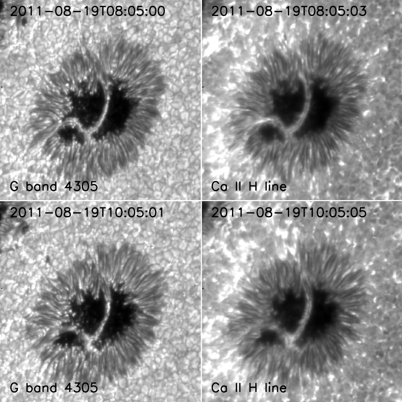
Figure 1: Two images in the first column are G band 4305 observed at 08:05:00 and 10:05:01 UT on 18 Aug 2011, respectively. Two images in the second column are Ca II observed at 08:05:00 and 10:05:01 UT on 18 Aug 2011, respectively.

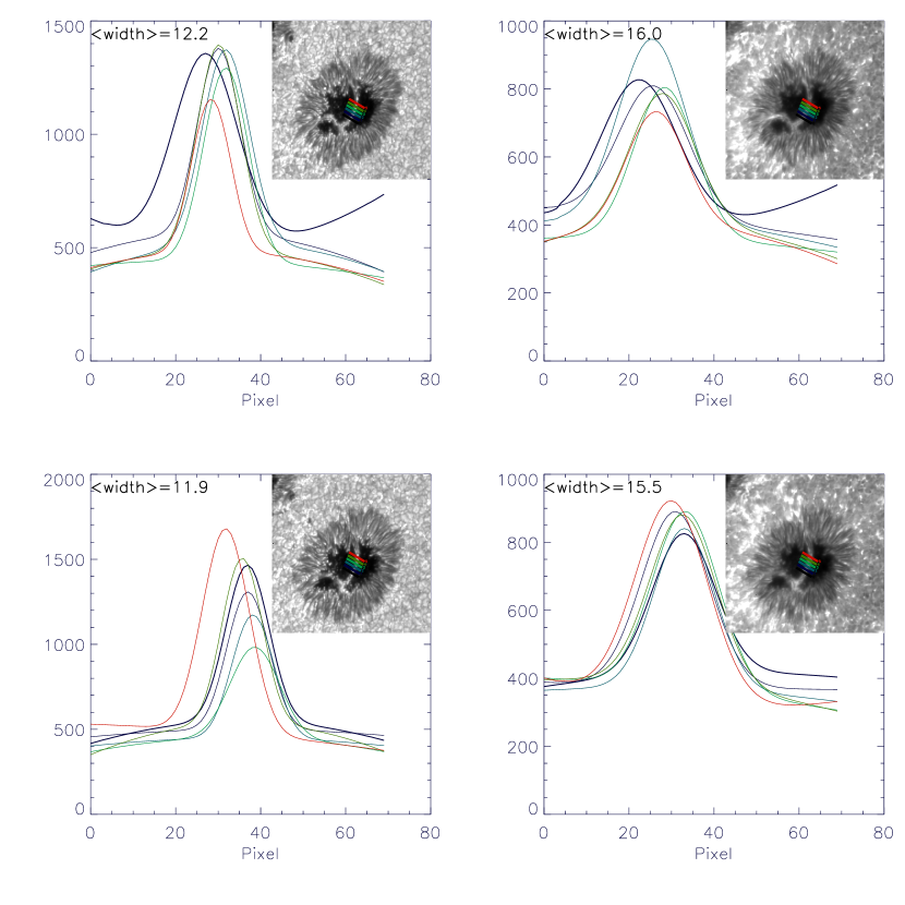
Figure 2: The figures to show the width of LB in images of G band 4305 and Ca II. The gray-scales in each column correspond images of 1, in each image there are six lines crossing LB that are plotted to display the width of LB, here the average of width with pixel unit are labeled.

Fig 1 shows G band 4305 and Ca II H images of this LB observed at two different time of 08:05:00 and 10:05:01 UT on 18 Aug 2011, respectively. Where the field of view is 45 arcsec $\times$ 45 arcsec, the first column and the second column shows G band 4305 images and Ca II H images, respectively. From this Figure, it can be seen that this LB should be classified ”umbral” LB according its intensity and fine structure, also it should be regarded as a strong one, since this LB penetrates the umbra completely and separates umbral core into two parts evidently. When it is seen more carefully, a evident ridge structure in the middle of LB along its length direction can be seen. This ridge structure display the dark features in these images, however it is more evidently displayed in Ca II H images. This maybe because the ridge structure locates at nearly the center position of LB in Ca II H images, while in G band images the position where ridge locates departed from the center position of LB. The ridge structure in G band images close to the west boundary of LB and the corresponding umbra. This observation confirm once again the previous results that the dark central lanes running along the length of LB.The width of LBs, which are $\sim$ 900/1150 km for Ca II H/G band observations, are calculated from these images Fig 2. In Fig 2, six lines crossing individual LB corresponding Fig 1 images are selected to calculated the width of LB, through calculation using GAUSS-FIT and regarding halfwidth as the width of LB, the color fit lines correspond individual line with the same color, respectively. The average of widths of LB in Ca II H/G band images about 12.1/15.8 pixel with the pixel size of 0.1 arcsec.

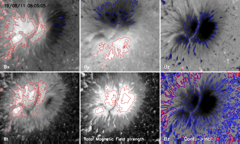
Figure 3: The images of magnetic component of $B_{x}$ with contour levels $\pm$800 and 1200 G, $B_{y}$ with contour levels $\pm$800 and 1200 G, $B_{z}$ with contour levels $\pm$1200 and 1500 G, $B_{t}$ (transverse magnetic field) with contour levels $\pm$1200 and 1500 G, $B_{tot.}$ (total magnetic field strength) with contour levels $\pm$2000 and 2500 G and the contour of inclination angle plotted on $B_{z}$ map with the contours levels $\pm$40^∘, 50^∘ and red/blue contours represent positive/negative values of inclination angle, the corresponding observation time is label.

In order to investigate LB magnetic field, Fig 3 shows magnetic components of $B_{x}$, $B_{y}$, $B_{z}$, the transverse magnetic field $B_{t}$ and total magnetic field strength $B_{tot.}$ for this LB observed time 08:05:05 UT. Basing on magnetic components the inclination angles of this LB are calculated, and the distribution of inclination angles (namely, atan($B_{t}/B_{z}$), where transverse magnetic field $B_{t}$ = $\sqrt{B_{x}^{2}+B_{y}^{2}}$) indicated by contour lines are plotted on the grey-scale map of $B_{z}$ in the last column of Fig 3. From Fig 3 it is can be found that the LB structures are seen clearly in image of each magnetic components of $B_{x}$, $B_{y}$ and $B_{z}$ and each deduced magnetic component. Here, the magnetic component of $B_{x}$ with contour levels $\pm$800 and 1200 G, $B_{y}$ with contour levels $\pm$800 and 1200 G, $B_{z}$ with contour levels $\pm$1200 and 1500 G, $B_{t}$ (transverse magnetic field) with contour levels $\pm$1200 and 1500 G, $B$ (total magnetic field strength) with contour levels $\pm$2000 and 2500 G, respectively. But for the inclination angles, the amplitudes of magnetic components ($B_{x}$, $B_{y}$, $B_{z}$, $B_{t}$ and $B_{tot.}$) of LB are all smaller than those of its neighboring umbra. As for the inclination angles, it is found that the inclination angles of LB are larger than those of neighboring umbra. Hence, the large value of inclination angles are shown as contour lines in Fig 3, where the contours are $\pm$40^∘, 50^∘ and red/blue contours represent positive/negative values of inclination angle, respectively. From the distribution of inclination angles, it can be found that the amplitude of inclination angles of LB are comparable to those of penumbra and a part of quiet regions. While there are less contour lines, which means less large value of inclination angles, exist at the region of umbra. In the images of $B_{x}$, $B_{y}$, $B_{z}$, $B_{t}$ and $B_{tot.}$, the relation between longitudinal and transverse magnetic field can not be clearly seen, but ratio of transverse field to longitudinal field that contained indirectly in inclination angles is higher than those of umbra, which also means that the magnetic field of LB are more inclined than those of umbra. However, here it should be noted that the total intensities of magnetic field of LB are weaker than those of umbra undoubtedly (see from the distributions of $B_{tot.}$).

To study magnetic field of LB, physical quantity force-free factor ($\alpha$) and z-component of current ($J_{z}$) and tension force ($T_{z}$) are calculated basing on the vector magnetograms observed at three different time. The definitions of $\alpha$, $J_{z}$ and $T_{z}$ are as follows:

From the basic electromagnetic equations force free factor ($\alpha$), current (J) and Lorentz force (F) can be expressed:

$$\alpha\emph{{B}}=\bigtriangledown\times\emph{{B}}=(\dfrac{\partial B_{z}}{\partial y}-\dfrac{\partial B_{y}}{\partial z})\emph{{i}}+(\dfrac{\partial B_{x}}{\partial z}-\dfrac{\partial B_{z}}{\partial x})\emph{{j}}+(\dfrac{\partial B_{y}}{\partial x}-\dfrac{\partial B_{x}}{\partial y})\emph{{k}},$$ (1)

$$\emph{{J}}=\dfrac{1}{\mu_{0}}\bigtriangledown\times\emph{{B}}=\dfrac{1}{\mu_{0}}[(\dfrac{\partial B_{z}}{\partial y}-\dfrac{\partial B_{y}}{\partial z})\textbf{\emph{i}}+(\dfrac{\partial B_{x}}{\partial z}-\dfrac{\partial B_{z}}{\partial x})\textbf{\emph{j}}+(\dfrac{\partial B_{y}}{\partial x}-\dfrac{\partial B_{x}}{\partial y})\textbf{\emph{k}}],$$ (2)

$$\emph{{F}}=\dfrac{(\emph{{B}}\centerdot\bigtriangledown)\emph{{B}}}{\mu_{0}}-\dfrac{\bigtriangledown(\emph{{B}}\centerdot\emph{{B}})}{2\mu_{0}}).$$ (3)

Where $\alpha$ can indicate the twist and current of field line at some extent. F can demonstrate the equilibrium of sunspots structure (Venkatakrishnan & Tiwari, 2010) at some extent. In equation 3, the first term is the tension force (T) and the second term represents the force due to magnetic pressure. Hence $\alpha$, z-component of current ($J_{z}$) and tension force ($T_{z}$) can be expressed as follows:

$$\alpha=(\dfrac{\partial B_{y}}{\partial x}-\dfrac{\partial B_{x}}{\partial y})/B_{z},$$ (4)

$$J_{z}=\dfrac{1}{\mu_{0}}(\dfrac{\partial B_{y}}{\partial x}-\dfrac{\partial B_{x}}{\partial y}).$$ (5)

$$T_{z}=\dfrac{1}{\mu_{0}}[B_{x}\dfrac{\partial B_{z}}{\partial x}+B_{y}\dfrac{\partial B_{z}}{\partial y}-B_{z}(\dfrac{B_{x}}{\partial x}+\dfrac{B_{y}}{\partial y})].$$ (6)

At last, $\alpha$, $J_{z}$ and $T_{z}$ all can be obtained on the photosphere, since the horizontal derivatives of the vector magnetic field observed on the photosphere can be calculated.

Fig 4 shows the images of $\alpha$, $J_{z}$ and $T_{z}$ calculated from vector magnetic field at three different observed time. For $\alpha$ in the first column, the contours are $\pm$0.008, 0.009 $m^{-1}$ and red/blue contours indicate positive/negative values of $\alpha$. It is found that $\alpha$ of LB are basic larger than those of its neighboring penumbra and umbra, however a large mount of large values of $\alpha$ are also dispersed in quiet regions. For $J_{z}$ second column, the contours are $\pm$0.08, 0.09 $Am^{-2}$ and red/blue contours represent positive/negative values, where the the positive/negative values means the direction of $J_{z}$ is up/down to the photosphere, respectively. On the whole it is found that $J_{z}$ of LB are larger than those of other parts including penumbra and umbra. Generally, it is found that one part of $J_{z}$ of LB have positive values and the other part have negative values, and this two are are divided at about the middle of LB along its length roughly (especially, seen evidently in the up panel in the second colume). For $T_{z}$ third column, the contours are $\pm$0.11, 0.12 $G^{2}m^{-1}$ and red/blue contours also represent positive/negative values of $\alpha$, and positive/negative contour lines also mean the direction of $T_{z}$ is up/down to the photosphere, respectively. Here the contour lines of $T_{z}$, which surround the boundary of LB and umbra, are plotted in this figure. It can be found that the direction of $T_{z}$ is opposite in LB and umbra. Additionally, an interested thing is that the change of direction of $T_{z}$ is exactly at the boundary between LB and umbra. This demonstrates that Lorentz force of boundary of LB has the trend up to the photosphere, while Lorentz force of boundary of umbra has the trend down to the photosphere. Hence, from the distribution of $T_{z}$ it can be found that magnetic system of LB and umbra should be regarded as two different systems. From Lorentz force equation (Eq.3), it can be seen that $T_{z}$ possibly is sensitive to the gradient of magnetic components. So in Fig 5 the relationships between $T_{z}$ and the gradient of magnetic components are shown by scatter diagrams tentatively, and the correlation coefficients are labeled respectively. It can be found that the large amplitudes $T_{z}$ (most of parts are negative values) correspond to small amplitudes of magnetic component gradient on the whole. While for small amplitudes of $T_{z}$ there are various amplitudes of magnetic component gradient can appear, then the amplitudes of magnetic components ($B_{x}$,$B_{y}$ and $B_{z}$ in Eq.3) may play relatively important contributions to $T_{z}$. The amplitude of $\alpha$, $J_{z}$ and $T_{z}$ in LB and other parts are calculated to see their differences related to position. Fig 6 shows the selected region of LB, umbra, penumbra and quiet region that labeled by blue closed lines, here the semi artificial method (IDL region-grow) are used to choose interested sub-region. It is found that the amplitude of $\alpha$ is about 0.007, 0.002, 0.004 and 0.100 $m^{-1}$ in LB, umbra, penumbra and quiet region, respectively. It is found that the amplitude of $J_{z}$ is about 0.05, 0.03, 0.04 and 0.05 $Am^{-2}$ in LB, umbra, penumbra and quiet region, respectively. It is found that the amplitude of $T_{z}$ is about 0.12, 0.30, 0.10 and 0.01 $G^{2}m^{-1}$ in LB, umbra, penumbra and quiet region, respectively.

4 Discussions and Conclusions

LBs are common magnetic feature during the evolution of sunspot, hence the magnetic properties of LBs can contribute the knowledge of sunspot magnetic field. Additionally, there are exist plentiful magnetic activities along LB and at the boundaries between LB and its neighboring umbra, such as chromospheric brighten, H$\alpha$ surge, corona jet and so on. Because the widths of LB are too narrow to be studied accurately by all current observations all most. Hence the formation, disappearances and properties of LB and also the interactions between LB and umbra are not known adequately. At present, the observatory of Hinode satellites is a high spatial resolution one. Although the spatial resolution of Hinode data maybe not high enough to study LB accurately, it gives us a good chance to maximum disclosure the fine properties of magnetic field and its related parameters.

In this paper, a LB existing in the lead sunspot of NOAA 11271 observed by Hinode satellites are presented and studied. Due to observations limitations (here 3 hours observation and gives 3 magnetograms available), the evolutions of LB are not reported in this paper, hence the object of this study should be regarded as a static LB neglecting its evolutions. The fine magnetic structures and features about LB are the main objects that we want to study in this paper, hence the main works done are targeted to the physical information related to magnetic field of LB and its neighboring penumbra and umbra. The physical quantities of force-free factor ($\alpha$) and z-component of current ($J_{z}$) and tension force ($T_{z}$), which related to magnetic field and can be deduced from vector magnetic field observed, are studied specially for this LB.

From the distributions and the amplitudes of $\alpha$, $J_{z}$ and $T_{z}$ in different parts (namely penumbra, umbra, LB and quiet region of this active region). it is found that the $\alpha$, $J_{z}$ and $T_{z}$ of LB are evidently different from those of its surrounding penumbra and umbra. $\alpha$, $J_{z}$ of LB are larger than those of its surrounding penumbra and umbra generally. $T_{z}$ of LB are smaller than those of its neighboring umbra, and the change of sign of $T_{z}$ at the boundary of LB and umbra is very obvious. These observation results may suggest that magnetic system of LB and its neighboring umbra (including penumbra) are two different magnetic systems. The magnetic topologies and environment of LB and its neighboring umbra are more suitable to create interactions between these two magnetic systems, such as magnetic reconnection. For example, the directions of tension force $T_{z}$ of LB and umbra are opposite, thus, there may exist easily the instabilities and interactions between these two different magnetic systems, which may create conditions for the consumptions of magnetic flux or the redistributions of magnetic field and then result in the breakup or assembly of sunspots.

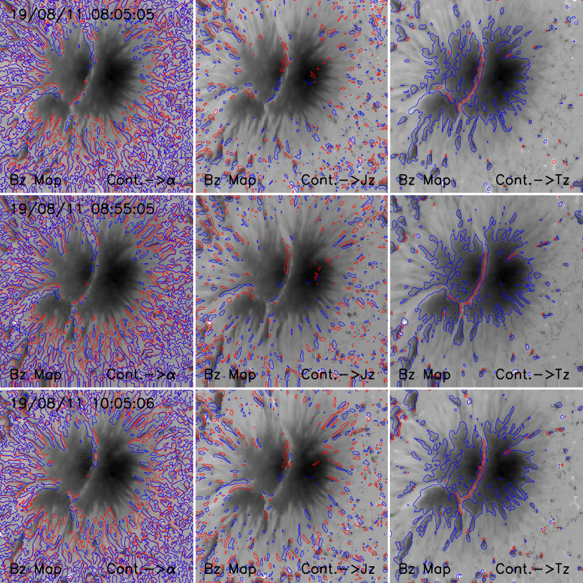
Figure 4: The background image are $B_{z}$ map and contour lines represent for the distribution of $\alpha$, $J_{z}$ and $T_{z}$, respectively. For $\alpha$ in the first column, the contours are $\pm$0.008, 0.009 $m^{-1}$ and red/blue contours represent positive/negative values. For $J_{z}$ in the second column, the contours are $\pm$0.08, 0.09 $Am^{-2}$ and red/blue contours represent positive/negative values. For $T_{z}$ in the third column, the contours are $\pm$0.11, 0.12 $G^{2}m^{-1}$ and red/blue contours represent positive/negative values. For vector $J_{z}$ and $T_{z}$, the positive/negative values means the direction of this vector is up/down to the photosphere, respectively

Figure 5: The scatter diagrams to show the relationships between $T_{z}$ and the gradient of magnetic components, where the gradient of magnetic components are labeled correspondingly.

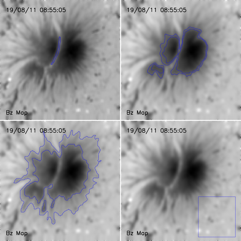
Figure 6: It shows the selected region of LB, umbra, penumbra and quiet region labeled by blue closed lines, here the semi artificial method (IDL region-grow) are used to choose interested sub-region.

aastex-help@aas.org.

References

- Asai (2001) Asai, A., Ishii, T.T., & Kurokawa, H. 2001, ApJ, 555, L65
- Berger & Berdyugina (2003) Berger, T.E. & Berdyugina, S.V. 2003, ApJ, 589, L117
- Bharti et al. (2007) Bharti, T., Rimmele, T., Jain, R., Jaaffrey, S.N.A., & Smart, R.N. 2007, MNRAS, 376, 1291
- Bray et al. (1964) Bray, R.J. & Loughhead, R.E. 1964, Sunspots, The International Astrophysics Series (London: Chapman & Hall)
- Garcia de La Rosa (1987) Garcia de La Rosa, J.I. 1987, Sol. Phys., 112, 49
- Garcia de La Rosa (1987) Garcia de La Rosa, J.I. 1987, Sol. Phys., 112, 49
- Jurcak et al. (2006) Jurcak, J., Pillet, V.M., & Sobotka, M. 2006, A&A, 112, 49
- Katsukawa (2007) Katsukawa, Y. 2007, New Solar Physics with Solar-B Mission ASP Conference Series, Edited by Kazunari Shibata, Shin’ichi Nagata, Takashi Sakurai, 369, p.287
- Katsukawa et al. (2007b) Katsukawa, Y., Yokoyama, T., Berger, T.E., Ichimoto, K., Kubo, M., Lites, B.W., Nagata, S., Shimizu, T., A.Shine, R., Suematsu, Y., D.Tarbell, T., M.Title, A. & Sueta, S. Katsukawa, Y., 2007, PASJ, 59, 577
- Kosugi et al. (2007) Kosugi, T., Matsuzaki, K., Sakao, T., Shimizu, T., Sone, Y., Tachikawa, S., Hashimoto, T., Minesugi, K., Ohnishi, A., Yamada, T., Tsuneta, S., Hara, H., Ichimoto, K., Suematsu, Y., Shimojo, M., Watanabe, T., Davis, J.M., Hill, L.D., Owens, J.K., Title, A.M., Culhane, J.L., Harra, L., Doschek, G.A., & Golub, L. 2007, Sol. Phys., 243, 3
- Leka (1997) Leka, K.D. 1997, ApJ, 484, 900
- Liu (2011) Liu, S. 2011, PASA, online
- Muller (1979) Muller, R. 1979, Sol. Phys., 61, 297
- Ravindra et al. (2011) Ravindra, B., Venkatakrishnan, P., Tiwari, S.K. & Bhattacharyya, R. 2011, ApJ, 740, 19
- Roy (1973) Roy, J.-R. 1973, Sol. Phys., 28, 95
- Rudenko & Anfinogentov (2014) Rudenko, G. V. & Anfinogentov, S. A. 2014, Sol. Phys., 289, 1499
- Ruedi et al. (1995) Ruedi, I., Solanki, S.K. & Livingston, W. 1979, Sol. Phys., 61, 297
- Ryutova et al. (2008) Ryutova, M., Berger, T., & Title, A. 2008, ApJ, 676, 1356
- Schmieder et al. (1994) Schmieder, B., Hagyard, M. J., Ai, G.X., Zhang, H.Q., Kalman, B., Gyori, L., Rompolt, B., Demoulin, P. & Machado, M. E. 1994, Sol. Phys., 150, 199
- Sobotka et al. (1993) Sobotka, M., Bonet, J.A. & Vazquez, M. 1993, ApJ, 415, 832
- Sobotka et al. (1994) Sobotka, M., Bonet, J.A. & Vazquez, M. 1994, ApJ, 426, 404
- Shimizu et al. (2009) Shimizu, T., Katsukawa, Y., Kubo, M., Lites, B.W., Ichimoto, K., Suematsu, Y., Tsuneta, S., Nagata, S., A.Shine, R., & D.Tarbell, T. 2009, ApJ, 696, L66
- Tanaka & Nakagawa (1973) Tanaka, K. & Nakagawa, Y. 1973, Sol. Phys., 33, 187
- Tiwari et al. (2009) Tiwari, S.T., Venkatakrishnan, P. & Sankarasubramanian, K. 2009, ApJ, 702, L133
- Su et al. (2010) Su, J.T., Liu, Y., Zhang, H.Q., Mao, X.J., Zhang, Y. & He, H. 2010, ApJ, 170, 710
- Lites et al. (1999) Lites, B. W., Rutten, R. J., Berger, T. E. 1999, ApJ, 517, 1013.
- Spruit & Scharmer (2006) Spruit, H.C., & Scharmer, G.B. 2006, ApJ, 415, 832
- Tsuneta et al. (2008) Tsuneta, S., Suematsu, Y., Ichimoto, K., Shimizu, T., Otsubo, M., Nagata, S., Katsukawa, Y., Title, A., Tarbell, T., Shine, R., Rosenberg, B., Hoffmann, C., Jurcevich, B., Levay, M., Lites, B., Elmore, D., Matsushita, T., Kawaguchi, N., Mikami, I., Shimada, S., Hill, L., & Owens, J. 2008, Sol. Phys., 249, 167
- Wang et al. (2008) Wang, H.M., Jing, J., Tan, C.Y., Wiegelmann, T. & Kubo, M. 2008, ApJ, 687, 658
- Vasquez (1973) Vasquez, M. 1973, Sol. Phys., 31, 377
- Venkatakrishnan & Tiwari (2010) Venkatakrishnan, P. & Tiwari, S. K. 2010, A&A, 516, L5
- Venkatakrishnan et al. (1993) Venkatakrishnan, P., Narayanan, R. S., & Prasad, N. D. N. 1993, Sol. Phys., 144, 315
- Zhang (2010) Zhang, H.Q. 2010, ApJ, 716, 1493