Projection-Based 2.5D U-net Architecture for Fast Volumetric Segmentation

Abstract

Convolutional neural networks are state-of-the-art for various segmentation tasks. While for 2D images these networks are also computationally efficient, 3D convolutions have huge storage requirements and require long training time. To overcome this issue, we introduce a network structure for volumetric data without 3D convolutional layers. The main idea is to include maximum intensity projections from different directions to transform the volumetric data to a sequence of images, where each image contains information of the full data. We then apply 2D convolutions to these projection images and lift them again to volumetric data using a trainable reconstruction algorithm. The proposed network architecture has less storage requirements than network structures using 3D convolutions. For a tested binary segmentation task, it even shows better performance than the 3D U-net and can be trained much faster.

1 Introduction

Deep convolutional neural networks have become a powerful method for image recognition ([1, 2]) . In the last few years they also exceeded the state-of-the-art in providing segmentation masks for images. In [3], the idea of transforming VGG-nets [2] to deep convolutional filters to obtain semantic segmentations of 2D images came up. Based on these deep convolutional filters, the authors of [4] introduced a novel network architecture, the so-called U-net. With this architecture they redefined the state-of-the-art in 2D image segmentation till today. The U-net provides a powerful 2D segmentation tool for biomedical applications, since it has been demonstrated to learn highly accurate ground truth masks from only very few training samples.

Among others, the fully automated generation of volumetric segmentation masks becomes increasingly important for biomedical applications. This task still is challenging. One idea is to extend the U-net structure to volumetric data by using 3D convolutions, as has been proposed in [5, 6]. Essential drawbacks are the huge memory requirements and long training time. Deep learning segmentation methods therefore are often applied to 2D slice images (compare [5]). However, these slice images do not contain information of the full 3D data which makes the segmentation task much more challenging.

To address the drawbacks of existing approaches, we introduce a network structure which is able to generate accurate volumetric segmentation masks of very large 3D volumes. The main idea is to integrate maximum intensity projection (MIP) layers from different directions which transform the data to 2D images containing information of the full 3D image. As an example, we test the network for segmenting blood vessels (arteries and veins) in magnetic resonance angiography (MRA) scans (Figure 1.1).

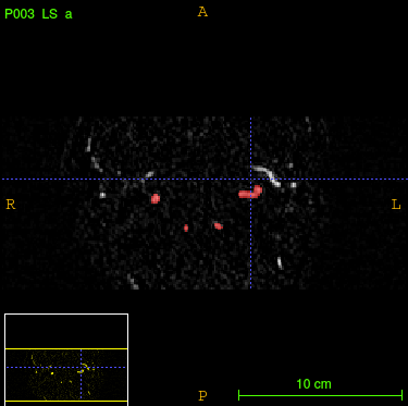
(a) Transversal.

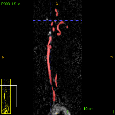
(b) Sagittal.

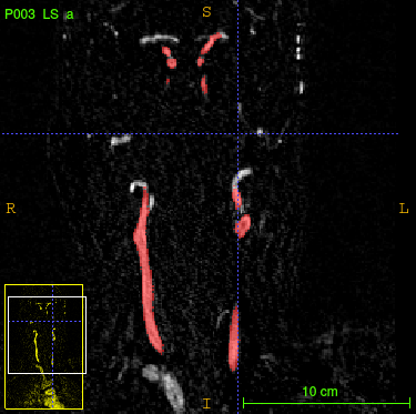
(c) Coronal.

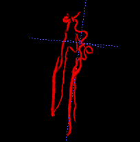
(d) 3D segmentation.

Figure 1.1: In every plane (a)-(c) the blood vessels of interest are marked in red. In (d) we see the corresponding 3D segmentation mask. The segmentation was conducted with the freeware ITK-SNAP [7].

The proposed network can be trained $15\times$ faster and requires order of magnitude less memory than networks with 3D convolutions, and still produces more accurate results.

2 Background

2.1 Volumetric segmentation of blood vessels

We aim at generating volumetric binary segmentation masks. In particular, as one targeted application, we aim at segmenting blood vessels (arteries and veins) which assists the doctor to detect abnormalities like stenosis or aneurysms. Furthermore, the medical sector is looking for a fully automated method to evaluate large cohorts in the future. The Department of Neuroradiology Innsbruck has provided volumetric MRA scans of 119 different patients. The images face the arteries and veins between the brain and the chest. Fortunately, also the volumetric segmentation masks (ground truths) of these 119 patients have been provided. These segmentation masks have been generated by hand which is long hard work (Figure 1.1).

Our goal is the fully automated generation of the 3D segmentation masks of the blood vessels. For that purpose we use deep learning and neural networks. At the first glance, this problem may seem to be quite easy because we only have two labels (0: background, 1: blood vessel). However, there are also arteries and veins which have label 0 which might confuse the network since we only want to segment those vessels of interest. Other challenges are caused by the big size of the volumes ($96\times 288\times 224$ voxels) and by the very unbalanced distribution of the two labels (in average, 99.76 % of all voxels indicate background).

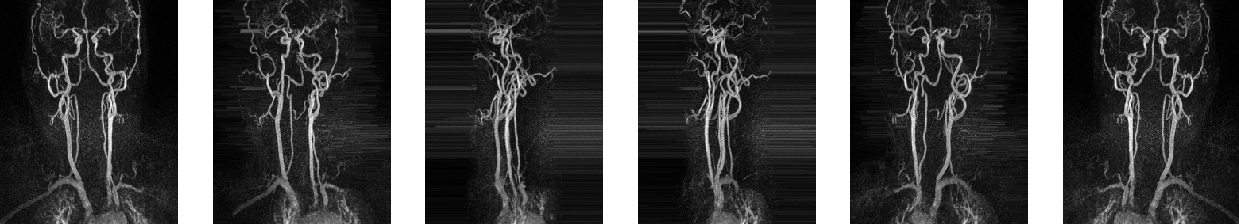
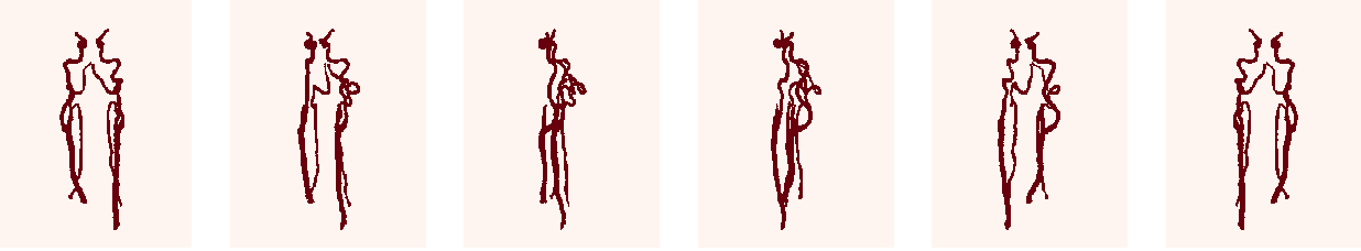
Figure 2.1: MIP images of a 3D MRA scan with $\alpha=36^{\circ}$. In the first row, we see the projections of the original scan, in the second row the corresponding projections of the ground truth.

2.2 Segmentation of MIP images

We first solve a 2D version of our problem. This can be done by applying maximum intensity projections to the 3D data and the corresponding 3D ground truths. Using a rotation angle of $\alpha=36^{\circ}$ around the vertical axis we obtain 10 MIP images out of each patient, which results in a data set to 1190 pairs of 2D images and corresponding 2D segmentation masks. Data corresponding for one patient are shown in Figure 2.1.

The U-net used for binary segmentation is a mapping $\mathcal{U}\colon\mathds{R}^{a\times b}\to[0,1]^{a\times b}$ which takes an image as input and outputs for each pixel the probability of being a foreground pixel. It is formed by the following ingredients [4]:

• The contracting part: It includes stacking over convolutional blocks (consisting of 2 convolutional layers) and max-pooling layers considering following properties: (1) We only use $3\times 3$ filters to hold down complexity and zero-padding to guarantee that all layer outputs have even spatial dimension. (2) Each max-pooling layer has stride $(2,2)$ to half the spatial sizes. We must be aware that the spatial dimensions of the input can get divided by 2 often enough without producing any rest. This can be done by slight cropping. (3) After each pooling layer we use twice as many filters as in the previous convolutional block.

• The upsampling part: To obtain similarity to the contracting part, we make use of transposed convolutions to double spatial dimension and to halve the number of filters. They are followed by convolutional blocks consisting of two convolutional layers with kernel size $3\times 3$ after each upsampling layer (compare Figure 2.2).

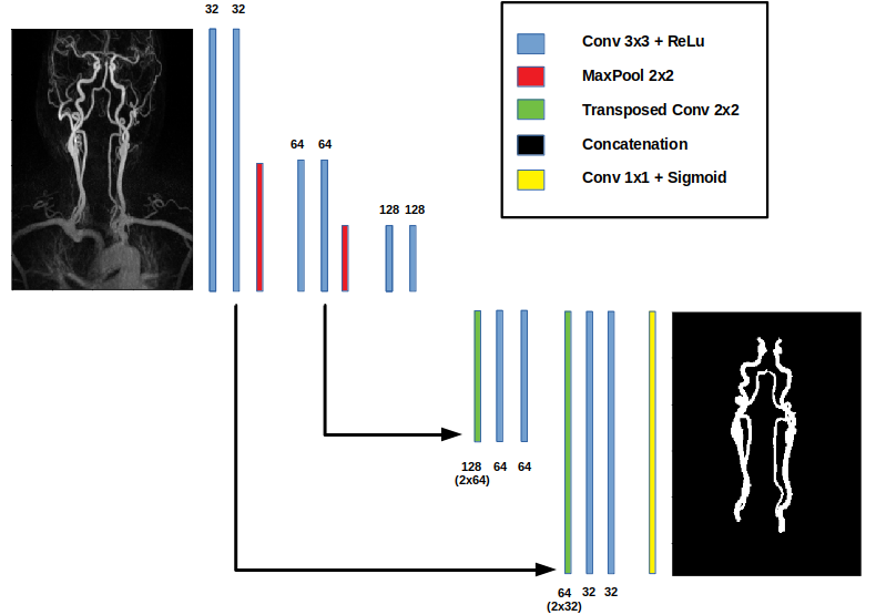
Figure 2.2: Visualization of the ground architecture of a 2D U-net.

Every convolutional layer in this structure gets followed by a ReLu-activation-function. To link the contracting and the upsampling part, concatenation layers are used, where two images with same spatial dimension get concatenated over their channel dimension (see Figure 2.2). This ensures a combination of each pixel’s information with its localization. At the end, the sigmoid-activation-function is applied, which outputs for each pixel the probability for being a foreground pixel. To get the final segmentation mask, a threshold (usually 0.5) is applied point-wise to the output of the U-net.
All networks in this paper are build with the Keras library [8] using Tensorflow backend [9]. Our implemented 2D U-net has filter size 32 at the beginning and filter size 512 at the end of the contracting part. The values of the start weights are normally distributed with expectation 0 and deviation $\frac{1}{f_{l}}$, where $f_{l}$ denotes the size of the $l$-th convolutional layer. The network is trained with the Dice-loss function [6]

$$\ell(y,\hat{y})=1-\frac{2\sum_{k}(y\odot\hat{y})_{k}}{\sum_{k}\hat{y}_{k}+\sum_{k}y_{k}},$$

where $\odot$ denotes pixelwise multiplication, the sums are taken over all pixel locations, $\hat{y}=\hat{f}(x)$ are the probabilities predicted by the U-net, and $y$ is the related ground truth. The Dice-loss function measures similarity by comparing all correctly predicted vessels pixels with the total number of vessels pixels in the prediction.

For $i,j\in\{0,1\}$ let us denote by $p_{ij}$ the set of all pixels of class $i$ predicted to class $j$, and by $t_{i}$ the number of all pixels belonging to class $i$. With this notation, we evaluate the following metrics during training:

• Mean Accuracy:

  $$\textbf{MA}\triangleq\frac{1}{2}\left(\frac{p_{00}}{t_{0}}+\frac{p_{11}}{t_{1}}\right)\,,$$

• Mean Intersection over Union [10]:

  $$\textbf{IU}\triangleq\frac{1}{2}\left(\frac{p_{00}}{t_{0}+p_{10}}+\frac{p_{11}}{t_{1}+p_{01}}\right)\,,$$

• Dice-coefficient ([6, 11]):

  $$\textbf{DC}\triangleq\frac{2p_{11}}{2p_{11}+p_{01}+p_{10}}\,.$$

To guarantee that all samples have satisfying spatial dimensions, the images get symmetrically cropped a little bit. We also make use of batch normalization layers [12] before each convolutional block to speed up convergence. To handle overfitting [13], we also recommend the integration of dropout layers [14] with dropout rate 0.5 in the deepest convolutional block and dropout rate 0.2 in the second deepest blocks. For training, Adam-optimizer [15] is used with learning rate 0.001 in combination with learning-rate-scheduling, i.e. if the validation loss does not decrease within 3 epochs the learning rate gets reduced by the factor 0.5. Furthermore, if the network shows no improvement for 5 epochs the training process gets stopped (early stopping) and the weights of the best epoch in terms of validation loss get restored. We use a (70, 15, 15) split in training, validation, and evaluation data and a threshold of 0.5 for the construction of the segmentation masks. Training the U-net on NVIDIA GeForce RTX 2080 GPU with a minibatch size of 6 yields the following results: Dice-loss of 0.088, mean accuracy of 95.7%, mean IU of 91.6%, and Dice-coefficient of 91.3%. In average, training the 2D U-net lasts 809 seconds, the application only 0.013 seconds. During training, the 2D U-net allocates a memory space of 1.7 gigabytes.

2.3 Segmentation with the 3D U-net

Now we aim at generating binary segmentation masks of sparse volumetric data using a 3D version of the prior introduced U-net. The resulting 3D U-net follows the same structure as in 2.2, the only difference is the usage of 3D convolutions and 3D pooling layers. For the 3D U-net we have to take special care about overfitting [13] and about memory space. Therefore, for the 3D U-net we have chosen filter size 4 at the beginning and filter size 16 at the end of the contracting part. Also the use of high dropout rates [14] (0.5 in the deepest convolutional block and 0.4 in the second deepest blocks) is necessary to ensure an efficient training process. Due to the huge size of our training samples ($96\times 288\times 224$ voxels), we train the network on batch, i.e. with minibatch size 1. During training the 3D U-net allocates more than 8 gigabyte memory space and therefore is not manageable any more by our GPU. Therefore, the training process on a AMD Ryzen 7 1700X eight-core processor takes in average 969 minutes. Since the number of 3D samples is only 119, we conducted 5 training-runs with random choice of training, validation and evaluation data. Using the 3D U-net we obtained in average following results: Dice-loss of 0.254, mean accuracy of 87.3%, mean IU of 80.5% and Dice-coefficient of 74.8%.

Although the 3D U-net demonstrates high precision in our application (see Figures 3.1,3.1), we are not satisfied with the long training time. In addition to it, we are very limited in the choice of convolutional layers and the corresponding number of filters due to the huge size of the input data. So it is hardly possible to conduct volumetric segmentation for even larger biomedical scans without using cropping or sliding-window techniques.

3 Projection-Based 2.5D U-net

As mentioned in the introduction, the naive approach for accelerating volumetric segmentation and reducing memory requirements is to process each of the 96 slice images independently through a 2D-network (compare [5]). However, this causes the loss of connection between the slice images. For our targeted application, applying the 2D U-net out of 2.2 to each slice image of the 3D MRA scans independently yields following disappointing results: Dice-loss of 0.849, mean accuracy of 54.5%, mean IU of 54.3%, and Dice-coefficient of 15.1%. Therefore we are looking for an alternative approach.

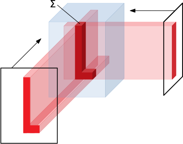
Figure 3.0(): Reconstruction operator $\mathcal{R}_{2}$: Voxel value is defined as the sum over the corresponding 2D values, here illustrated for 2 MIP images with directions $\{0^{\circ},90^{\circ}\}$.

3.1 Proposed 2.5D U-net architecture

As we have seen in 2.2, the 2D U-net does very well on the MIP images. Recall that a network for binary volumetric segmentation is a function $\mathcal{N}:\mathbb{R}^{a\times b\times c}\to[0,1]^{a\times b\times c}$ that maps the 3D scan to the probabilities that a voxel corresponds to the desired class. For a 3D input $x$, the proposed 2.5D U-net takes the form

$$\mathcal{N}({x})=\mathcal{T}\circ\mathcal{R}_{p}\circ\mathcal{F}_{p}\circ\begin{bmatrix}\mathcal{U}\circ\mathcal{M}_{\alpha_{1}}({x})\\ \vdots\\ \mathcal{U}\circ\mathcal{M}_{\alpha_{p}}({x})\end{bmatrix},$$ (3.1)

where

• $\mathcal{M}_{i}:\mathbb{R}^{a\times b\times c}\to\mathbb{R}^{b\times c}$ are MIP images for different projection directions ${\alpha_{1}},\ldots,{\alpha_{p}}$,

• $\mathcal{U}:\mathbb{R}^{b\times c}\to[0,1]^{b\times c}$ is the same 2D U-net as in 2.2 producing probabilities,

• $\mathcal{F}_{p}:([0,1]^{b\times c})^{p}\to(\mathbb{R}^{b\times c})^{p}$ is a learnable filtration,

• $\mathcal{R}_{p}:(\mathbb{R}^{b\times c})^{p}\to\mathbb{R}^{a\times b\times c}$ is a reconstruction operator using $p$ linear backprojections as shown in Figure 3,

• $\mathcal{T}:\mathbb{R}^{a\times b\times c}\to[0,1]^{a\times b\times c}$ is a fine-tuning operator (average pooling followed by a learnable shift-operator followed by the sigmoid-activation-function).

The backprojection operator $\mathcal{R}_{p}$ causes a kind of shroud (Figure 3.1), so we have to think about a filtrated backprojection. Therefore, we apply a convolutional layer $\mathcal{F}_{p}$ before backprojection. Using $1\times 3$ filters, which get adapted during training for each projection direction $\alpha_{1},\ldots,\alpha_{p}$ individually, leads to a more satisfying result (Figure 3.1).

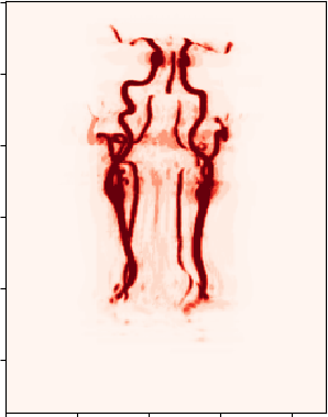
Figure 3.1(): Network’s output (before threshold) without filtration.

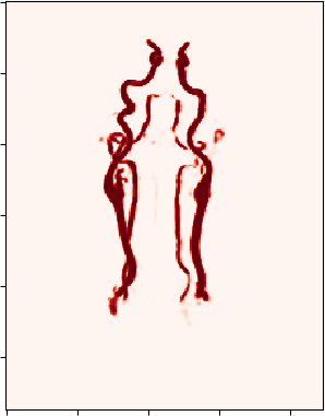
Figure 3.1(): Network’s output (before threshold) with filtration.

For the fine-tuning operator $\mathcal{T}$ we use average pooling with pool-size (2, 2, 2). This is followed by a learnable shift-operator, which shifts the pooled data by an adjusted parameter since the decision boundaries have been changed by $\mathcal{R}_{p}$. This ensures, that the application of the sigmoid function delivers accurate probabilities.

For our targeted application, again we only process one 3D sample through the network per iteration (minibatch size 1). The start weights of the convolutional part $\mathcal{U}$ in 3.1 are initialized in the same way as in Section2.2. The parameters of $\mathcal{F}_{p}$ and $\mathcal{T}$ are initialized empirically.

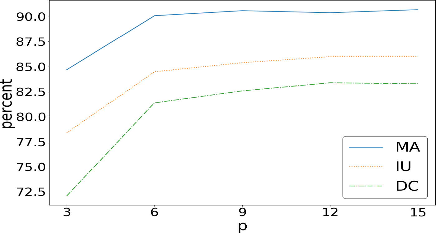
Figure 3.2: Performance of the 2.5D U-net for different number $p$ of projection directions .

For the amount of the projection directions we choose equidistant angles $\Theta=\{k\times\frac{180}{p}\mid k=0,\ldots,p-1\}$ to ensure we obtain at most different information of the 3D data for different projection directions. This causes the task of finding the best value for $p$ in 3.1. Therefore we trained the proposed network $\mathcal{N}$ for different values for $p$ and compared performance in terms of the evaluation metrics (Figure 3.2).

Looking at Figure 3.2, we observe that $\Theta=\{k\times\frac{180}{12}\mid k=0,\ldots,11\}$ seems to be a good choice for the amount of projection directions. We have conducted 5 training runs with random choice of training, validation and evaluation data and obtained in average following results: Dice-loss of 0.201, mean accuracy of 91.6 %, mean IU of 86.1 % and Dice-coefficient of 83.7 %.

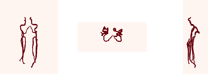
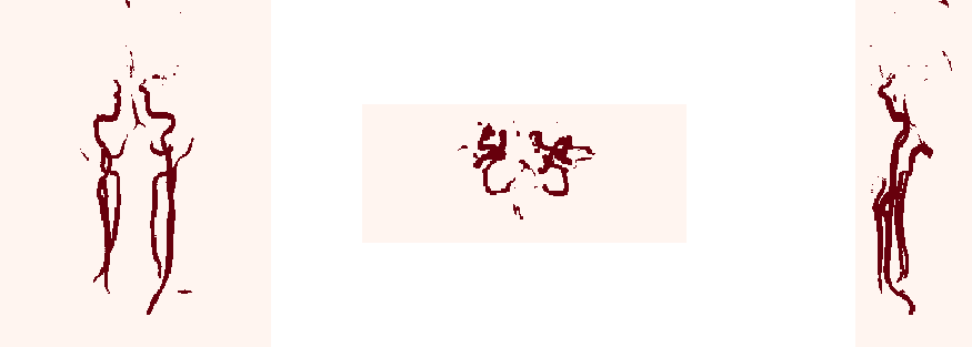
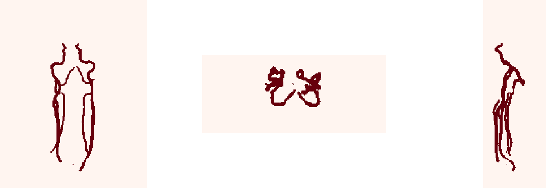
Figure 3.2(): Comparison between ground truth (first row), segmentation generated by 3D U-net (second row) and segmentation generated by 2.5D U-net (third row).

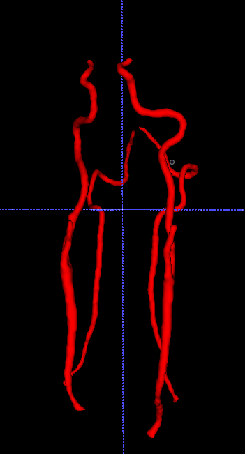
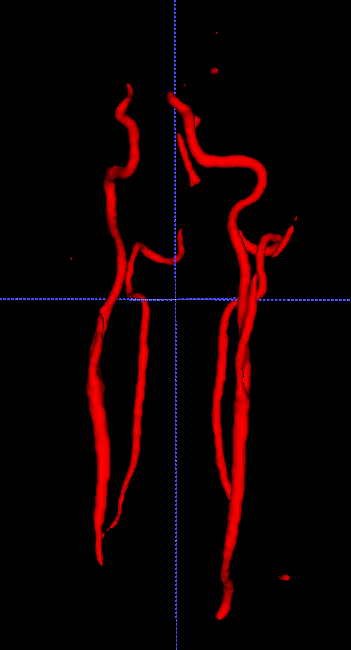
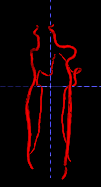
Figure 3.2(): 3D segmentation mask generated by hand (left), by 3D U-net (middle) and by 2.5D U-net (right).

As we can see, for the volumetric segmentation of MRA scans the proposed 2.5D U-net clearly outperforms 3D U-net in terms of evaluation metrics. Furthermore, adjusting the weights of 2.5D U-net only takes in average 3914 seconds. With 11.37 seconds, the application time increased due to the construction of the MIP images. During training, the 2.5D U-net allocates a memory space of 3.7 gigabytes.
Further tasks would be to investigate if applying data augmentation techniques to the 3D samples increases accuracy of the 3D U-net. Considering our application, data deformation could cause problems due to the fact, that the orientation of the vessels has huge impact to the network’s prediction. We will investigate that in the future.

Table 1: Summarization of the evaluation results for the naive 2D U-net slice-per-slice approach, the 3D U-net and the proposed 2.5D U-net.

Network	loss	MA in %	IU in %	DC in %
2D U-net	0.849	54.5	54.3	15.1
3D U-net	0.254	87.3	80.5	74.8
2.5D U-net	0.201	91.6	86.1	83.7

Table 2: Summarization of time and storage observations for the naive 2D U-net slice-per-slice approach, the 3D U-net and the proposed 2.5D U-net..

Network	Weights	Train	Appl.	Mem.
2D U-net	$8.6\times 10^{6}$	809 sec.	1.83 sec.	1.7 Gb
3D U-net	$2.5\times 10^{4}$	58140 sec.	5.28 sec.	$>8$ Gb
2.5D U-net	$8.6\times 10^{6}$	3914 sec.	11.37 sec.	3.7 Gb

4 Conclusion

In this paper we proposed a new projection-based 2.5D U-net structure for fast volumetric segmentation. The construction of volumetric segmentation masks with the help of a 3D U-net delivers very satisfying results, but the long training time and the big need of memory space are hardly sustainable. The 2.5D U-net using 12 deterministic projection directions is able to conduct 3D segmentation of very big biomedical 3D scans as reliable as the 3D U-net and can be trained much faster without any concern about memory space. For our targeted application, the 2.5D U-net enables the generation of 3D segmentations in a storage efficient way more accurate than other approaches using 3D convolutions and can be trained almost $15\times$ faster. All numerical results considering the evaluation metrics are displayed in Table 1. Average training time, application time and storage requirements for each network are summarized in Table 2. In the current implementation, we only use MIP images for deterministic projection directions. In future work, we will investigate the use of random projection directions for network training. This could provide the possibility to use all available information from each projection direction for the construction of 3D segmentation masks. Also the conduction of comparative studies will be a future task with the aim to research, if the 2.5D U-net also increases accuracy in other applications compared to 3D convolutions.

References

- [1] K. He, X. Zhang, S. Ren, and J. Sun, “Deep residual learning for image recognition,” in Proceedings of the IEEE conference on computer vision and pattern recognition, 2016, pp. 770–778.
- [2] K. Simonyan and A. Zisserman, “Very deep convolutional networks for large-scale image recognition,” arXiv preprint arXiv:1409.1556, 2014.
- [3] J. Long, E. Shelhamer, and T. Darrell, “Fully convolutional networks for semantic segmentation,” in Proceedings of the IEEE conference on computer vision and pattern recognition, 2015, pp. 3431–3440.
- [4] O. Ronneberger, P. Fischer, and T. Brox, “U-net: Convolutional networks for biomedical image segmentation,” in International Conference on Medical image computing and computer-assisted intervention. Springer, 2015, pp. 234–241.
- [5] Ö. Çiçek, A. Abdulkadir, S. S. Lienkamp, T. Brox, and O. Ronneberger, “3D U-net: learning dense volumetric segmentation from sparse annotation,” in International conference on medical image computing and computer-assisted intervention. Springer, 2016, pp. 424–432.
- [6] B. Erden, N. Gamboa, and S. Wood, “3D convolutional neural network for brain tumor segmentation,” 2018.
- [7] P. A. Yushkevich, J. Piven, H. Cody Hazlett, R. Gimpel Smith, S. Ho, J. C. Gee, and G. Gerig, “User-guided 3D active contour segmentation of anatomical structures: Significantly improved efficiency and reliability,” Neuroimage, vol. 31, no. 3, pp. 1116–1128, 2006.
- [8] F. Chollet et al., “Keras,” https://keras.io, 2015.
- [9] M. Abadi, A. Agarwal, P. Barham, E. Brevdo, Z. Chen, C. Citro, G. S. Corrado, A. Davis, J. Dean, M. Devin, S. Ghemawat, I. Goodfellow, A. Harp, G. Irving, M. Isard, Y. Jia, R. Jozefowicz, L. Kaiser, M. Kudlur, J. Levenberg, D. Mané, R. Monga, S. Moore, D. Murray, C. Olah, M. Schuster, J. Shlens, B. Steiner, I. Sutskever, K. Talwar, P. Tucker, V. Vanhoucke, V. Vasudevan, F. Viégas, O. Vinyals, P. Warden, M. Wattenberg, M. Wicke, Y. Yu, and X. Zheng, “TensorFlow: Large-scale machine learning on heterogeneous systems,” 2015, software available from tensorflow.org. [Online]. Available: http://tensorflow.org/
- [10] A. Rosebrock, “Intersection over union (IOU) for object detection,” https://www.pyimagesearch.com/2016/11/07/intersection-over-union-iou-for-object-detection/, 2016, last accessed: 2019-04-29.
- [11] L. R. Dice, “Measures of the amount of ecologic association between species,” Ecology, vol. 26, no. 3, pp. 297–302, 1945.
- [12] S. Ioffe and C. Szegedy, “Batch normalization: Accelerating deep network training by reducing internal covariate shift,” arXiv preprint arXiv:1502.03167, 2015.
- [13] I. Goodfellow, Y. Bengio, and A. Courville, Deep learning. MIT press, 2016.
- [14] N. Srivastava, G. Hinton, A. Krizhevsky, I. Sutskever, and R. Salakhutdinov, “Dropout: a simple way to prevent neural networks from overfitting,” The Journal of Machine Learning Research, vol. 15, no. 1, pp. 1929–1958, 2014.
- [15] J. Brownlee, “Gentle introduction to the adam optimization algorithm for deep learning,” https://machinelearningmastery.com/adam-optimization-algorithm-for-deep-learning/, 2017, last accessed: 2019-01-29.