Topography of (exo)planets

Abstract

Current technology is not able to map the topography of rocky exoplanets, simply because the objects are too faint and far away to resolve them. Nevertheless, indirect effect of topography should be soon observable thanks to photometry techniques, and the possibility of detecting specular reflections. In addition, topography may have a strong effect on Earth-like exoplanet climates because oceans and mountains affect the distribution of clouds (Houze, 2012). Also topography is critical for evaluating surface habitability (Dohm and Maruyama, 2015).

We propose here a general statistical theory to describe and generate realistic synthetic topographies of rocky exoplanetary bodies. In the solar system, we have examined the best-known bodies: the Earth, Moon, Mars and Mercury. It turns out that despite their differences, they all can be described by multifractral statistics, although with different parameters. Assuming that this property is universal, we propose here a model to simulate 2D spherical random field that mimics a rocky planetary body in a stellar system. We also propose to apply this model to estimate the statistics of oceans and continents to help to better assess the habitability of distant worlds.

Affiliations:

(1) GEOPS, Univ. Paris-Sud, CNRS, Université Paris Saclay, Rue du Belvedere, Bat. 504–509, 91405 Orsay, France (2) Physics department, McGill University, 3600 University st., Montreal, Que. H3A 2T8, Canada

*Correspondence to:

F. Landais (francois.landais@u-psud.fr) Keywords: planetary systems, planets and satellites: surfaces, planets and satellites: terrestrial planets, methods: numerical

1 Introduction

Efforts to detect and study exoplanets in other solar systems were initially restricted to gas giants (Mayor and Queloz, 1995) but multiple rocky exoplanets have now been discovered (Wordsworth et al., 2011). Their climates depend mainly on their atmospheric composition, stellar flux and orbital parameters (Wang et al., 2014; Forget and Leconte, 2014). But topography also plays a role in atmospheric circulation (Blumsack, 1971) and is an important trigger for cloud formation (Houze, 2012). Furthermore, the presence of an ocean filled with volatile compounds at low albedo is of a prime importance to the climate (Charnay et al., 2013). Last but not least, surface habitability relies on the presence of the three elements: the atmosphere, ocean and land (Dohm and Maruyama, 2015). Topography is also the determinant of ocean and land cover.

Thanks to different observations techniques, measurements of the atmospheres of hot Jupiter planets have been achieved (Seager, 2010). Significantly, the detection of clouds has been reported (Demory et al., 2013) indicating strong heterogeneity in their spatial distribution. The detection of the first atmospheric transmission spectra of a super-Earth (Bean et al., 2010) and the discovery of a rocky exoplanet in the habitable zone around a dwarf star opens a new area in exoplanet science (de Wit et al., 2016). Such observations are expected to be increasingly frequent (Tian, 2015). Nevertheless, with current technology, direct imaging of exoplanets is very difficult because the objects are too faint and too far away. For the moment, the only way to determine the topography is by statistical models.

In the near future, photometry techniques should improve our knowledge of exoplanet topography , even if the bodies are not resolved in ways similar to the small bodies in our Solar System (see for instance Lowry et al. (2012) for estimates of the shape of comet 67P before the Rosetta landing). In addition, if oceans or lakes are present, their specular reflection should be detectable , for example, as also observed through the haze of Titan (Stephan et al., 2010) . Even if exoplanets are too far to be resolved, their topographies should be studied now. We offer here a framework to prepare and interpret future observations.

Recently, we reported the first unifying statistical similarity between the topographic fields of the best known bodies in the Solar System: Earth, Moon, Mars and Mercury (Landais et al., 2018). All these topographies seems to be well described by a mathematical scaling framework called «multifractals». The multifractal model, initially proposed for topography by Lavallee et al. (1993) describes the distribution and correlation of slopes at different scales. More precisely, we consider here the “universal multifractal” model developed by Schertzer and Lovejoy (1987). The accuracy of such a model has been tested in the case of different available topographic fields on Earth (Gagnon et al., 2006), Mars (Landais et al., 2015), Mercury and the Moon (Landais et al., 2018). This model has the advantage to reproduce closely the statistical properties of natural topography: the scaling properties, but also the intermittency (both rough and smooth regions can be found on the planets). Universal multifractals depend on only 3 parameters: $H$ controls how the roughness changes from one scale to another and $C_{1}$ controls the spatial heterogeneity of the roughness near the mean and $\alpha$ quantifies how rapidly the properties change as we move away from the mean topographic level. The bodies studied show transitions at ~10 km and are characterized by specific multifractal parameters (Landais et al., 2018). The scaling law at large scales (> 10 km) is characterized for the Moon by $H=0.2$, Mercury by $H=0.3$, Mars and Earth by $H=0.5$. The $\alpha\sim 1.9$ for the Earth, Mars and Mercury but $\alpha\sim 1.4$ for the Moon. The $C_{1}\sim 0.1$ for Earth and Mars, with lower values $C_{1}\sim 0.06$ for Mercury and $C_{1}\sim 0.03$ for the Moon. These differences are interpreted to be linked to dynamical topography and variation of elastic thickness of the crust (see table 1).

Assuming that exoplanets are statistically similar to those observed in our own Solar System, we propose here a stochastic topographic model. Such models will be very useful for investigating the distribution of exoplanet oceans, for studying the effect of topography on exoplanet climates, and for studying the effect of topography on their orbital motions or for determining the effect of topography and roughness on photometry. It can also be used to study the early climate on Earth.

The purpose of this article to first present our statistical model and its implementation on the sphere we then discuss the distribution of oceans and land cover. An introduction to the multifractal formalism can be found in the next section.

2 Method

2.1 Universal multifractals

The first application of fractional dimensions on topography was by B. Mandelbrot in his article “how long is the coast of Britain” (Mandelbrot, 1967). Fractals are geometrical sets of points that have scaling, power law, deterministic or statistical relations from one scale to another. This type of behavior has been observed in geophysical phenomenon including turbulence - clouds, wind, ocean gyres - but also faults in rock, geogravity, geomagnetism and topography (Lovejoy and Schertzer, 2007)

. The most common way to test scaling is to study the dependence of various statistics as functions of scale. Topographic level contours (isoheights) are fractals if for example the length of the contour is a power law function of the resolution at which it is measured. In this case, the level set is “scaling” and the exponent is its fractal dimension. In real topography, each level set has its own different fractal dimension so that the topography itself is a multifractal (Lavallee et al., 1993). Numerous studies haves shown that in several contexts, topography is scaling over a significant range of scales (see the review in Lovejoy and Shertzer, 2013). If the topography is multifractal, fractal dimensions measured locally appear to vary from one location to another. Indeed multifractal fields can be thought as a hierarchy of singularities whose exponents are random variables. Modern developments have introduced the notion of multifractal processes for such fields. For such processes, a local estimate of a fractal exponent is expected be different from a location to another without requiring different processes to generate it. With multifractals, it is possible to interpret the topography of regions that exhibit completely different slope distributions in a unified statistical framework. These models suggest global topography analyses are relevant despite of their diversity and complexity. Previous studies (Gagnon et al., 2006; Lavallee et al., 1993) have established the accuracy of multifractal global statistical approach in the case of Earth’s topography. More precisely, a particular class of multifractal has been considered: the universal multifractal, a stable and attractive class (Schertzer and Lovejoy, 1987). In our previous analysis (Landais et al., 2015), we performed the same kind of global analysis on the topographic data from Mars, from MOLA laser altimeter measurement (Smith et al., 2001). This analysis also find a good agreement with universal multifractal but on a restricted range of scale (Landais et al., 2015). Indeed the statistical structure has been found to be different at small scale (monofractal) and large scale (multifractal) with a transition occurring around 10 km.

Fluctuations

In order to interpret topography as a multifractal, we must quantify its fluctuations. The simplest fluctuation that can be used to describe topography is the distribution of changes in altitude $\Delta h$ over horizontal distances $\Delta x$. There are many other ways to define fluctuations, the general framework being wavelets. The simple altitude difference corresponds to the so called “poor man’s” wavelet and can be efficiently replaced by the Haar wavelet that tends to converge faster and is useful over a wider range of geophysical process. Over an interval $\Delta x$, the Haar fluctuation is the average elevation over the first half of the interval minus the average elevation over the second half (see Lovejoy, 2014; Lovejoy and Schertzer, 2012) and paragraph below for a precise definition of Haar fluctuations). The computation of fluctuations can be performed for each pair of elevation data in order to accumulate a huge amount of slope fluctuations. From this, a global planetary average $M(\Delta x)$ can be performed and will reflect the mean fluctuation of slopes at the scale $\Delta x$.

Scaling

By estimating fluctuations at different scales, we can observe the structure of the statistical dependance of the ensemble mean fluctuation at scale $\Delta x$: $M(\Delta x)$ . If the topographic field is fractal, this dependance is a power-law corresponding to equation 1 where H is a power law exponent (named in Honor of Ewin Hurst and equal to the Hurst exponent in the monofractal, Gaussian case):

$$M(\Delta x)\sim\Delta x^{H}$$ (1)

Statistical moments

Additionally, instead of simply considering the average (i. e.the first statistical moment of the fluctuations), we can compute any statistical moment $M_{q}$ of order $q$ defined by $M_{q}=<\Delta h^{q}>$ ; $M_{q}$ is called the $q^{\mathrm{th}}$ order structure function. If $q=2,$ it simply corresponds to the usual (variance based) structure function. In principle, all orders (including non-integer orders) must be computed to fully characterize the full variability of the data.

Multifractality

$M_{q}$ allows us to introduce two distinct statistical structures of interest: monofractal and multifractal. For a detailed description of the formalism we apply in this study, the readers can refer to Lovejoy and Shertzer (2013) briefly summed in Landais et al. (2015). We quickly recall the main notions here :

• In the monofractal case the parameters $H$ is sufficient to describe the statistics of all the moments of order $q$ (equation 2). In this case, no intermittency is expected, meaning that the roughness of the field is spatially homogenous despite of its fractal variability regarding to scales. Typically, the value $H=0.5$ corresponds to the classic Brownian motion. This kind of model has been used in many local and regional analysis of natural surfaces (Orosei et al., 2003; Rosenburg et al., 2011), but it fails to account for the intermittency (and strongly non-Gaussian statistics) commonly observed on large topographic datasets.

  $$M_{q}\sim\Delta x^{qH}$$ (2)

• In the multifractal case, $H$ is no longer sufficient to fully describe the statistics of the moments of order $q$. An additional convex function $K(q)$ depending on $q$ is required (3).

  $$M_{q}\sim\Delta x^{qH-K(q)};$$ (3)

• The moment scaling function $K$ modifies the scaling law of each moment. The consequence on the corresponding field appears clearly on simulations: the field exhibit a juxtaposition of rough and small places that are clearly more realistic in the case of natural surfaces (Gagnon et al., 2006). Moreover, it is possible to restrain the generality of the function $K(q)$ by considering universal multifractals, a stable and attractive class proposed by Schertzer and Lovejoy (1987) for which the multifractality is completely determined by the mean intermittency $C_{1}=\left(\frac{dK(q)}{dq}\right)_{q=1}$ (codimension of the mean) and the curvature $\alpha$ of the function $K$, $\alpha=\frac{1}{C_{1}}\frac{d^{2}K(q)}{dq^{2}}$ evaluated at $q=1$ (the degree of multifractality). In this case the expression of $K$ is simply given by equation 4

$$K(q)=\frac{C_{1}}{\alpha-1}(q^{\alpha}-q)$$ (4)

2.2 Spherical multifractal simulation

Simulations in 1D or 2D with multifractal properties and specific values for $\alpha$, $H$ and $C_{1}$ can be obtained by the procedure defined by Schertzer and Lovejoy (1987); Wilson et al. (1991). The necessary steps are briefly reminded here after :

• Step 1 : Generation of a un-correlated Levy noise $\gamma_{\alpha}(r)$. When $\alpha=2,$ it simplifies to a gaussian white noise whereas $\alpha<2$ corresponds to an extremal levy variable with negative extreme values.

• Step 2 : Convolution of $\gamma_{\alpha}(r)$ with a singularity $g_{\alpha}(r)$ defined by equation 5 to obtain a Levy-generator $\Gamma_{\alpha}(r)$, by using a convolution denoted by “$\star"$

  $$g_{\alpha}(r)=|r|^{-2/\alpha}$$ (5)

  $$\Gamma(r)=C_{1}^{1/\alpha}g(r)\star\gamma_{\alpha}(r)$$ (6)

• Step 3 : Exponentiation of the generator to obtain the multifractal noise $\varepsilon$

  $$\varepsilon=e^{\Gamma}$$ (7)

• Step 4 : The final field is then obtained by fractional integration of order H (another convolution similar to step 2)

Whereas the convolutions required for step 2 and 4 can easily be performed in Fourier space for the cartesian case, the generalization to spherical case is not straightforward, but as shown in appendix 5D of Lovejoy and Shertzer (2013), it can be done using spherical harmonics. Let $\theta$ and $\varphi$ being respectively the colatitude and longitude angle, the singularity can be expressed by equation 8. As it is symmetric by rotation along $\varphi$, $g_{\alpha}(\theta,\varphi)$ only depend on $\theta$.

$$g_{\alpha}(\theta,\varphi)=\theta^{-2/\alpha}$$ (8)

Let the spherical harmonic expansion of $g_{\alpha}(\theta,\varphi)$ be given by equation 9, where $Y_{lm}$ is the spherical harmonic of order $m$ and $l$. As $g_{\alpha}(\theta,\varphi)$ does not depend on $\varphi$, all the $Y_{lm}$ for $m\neq 0$ are equal to zero.

$$g_{\alpha}(\theta,\varphi)=\sum\sigma_{l}Y_{l,0}$$ (9)

Let the spherical harmonic expansion of $\gamma_{\alpha}(\theta,\varphi)$ be given by :

$$\gamma_{\alpha}(\theta,\varphi)=\sum u_{lm}Y_{l,m}(\theta,\varphi)$$ (10)

Then the convolution $C$ of $g_{\alpha}(\theta,\varphi)$ and $\gamma_{\alpha}(\theta,\varphi)$ is given by :

$$C=\sum_{l,m}\sigma_{l}\sqrt{\frac{4\pi}{2l+1}}u_{lm}Y_{l,m}(\theta,\varphi)$$ (11)

3 Results

3.1 Solar System

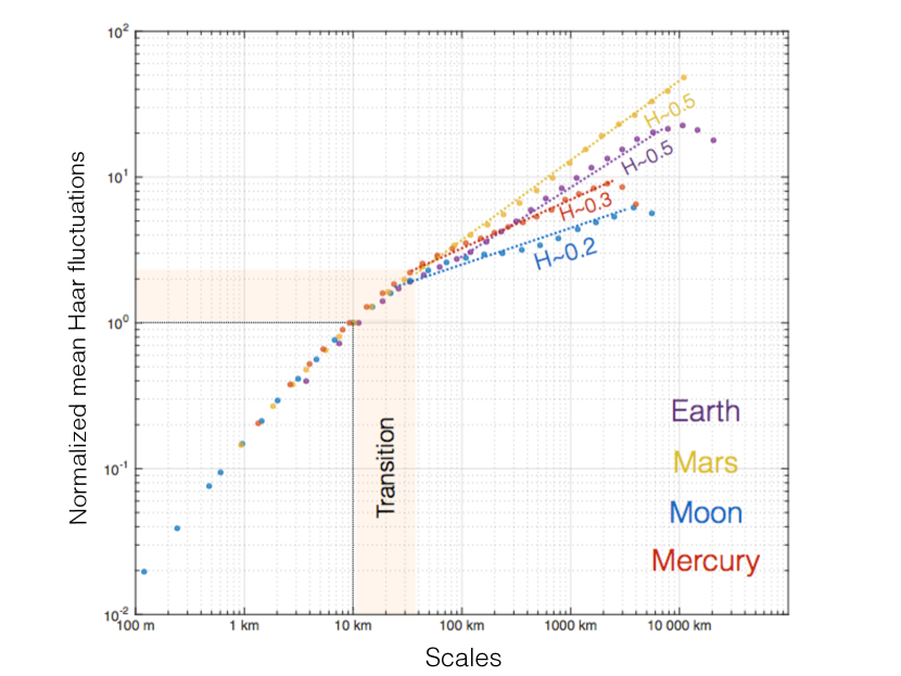
Figure 1: Mean fluctuations of topography of Earth, Mars, Moon and Mercury, as a function of scale. All dataset are normalized in order to be equal to 1 at the scale 10km. The normalization does not modify the scaling behavior but emphasize the transition occurring at around 10km. The errors bars are smaller than the size of the points.

In this section, we recall the main results of the planetary bodies of the Solar System. On Figure 1, we have plotted the mean normalized fluctuations of altitude as a function of scale on a log-log plot. The easiest way to define fluctuations at a given scale $\Delta x$ is to take the simple difference of altitude between two points separated by the distance $\Delta x$. We average all of these fluctuations over the whole planetary body. As we are focusing on statistical properties, the results on figure 1 have been normalized in order to emphasize the transition between 2 distinct range of scales. The global average have been normalized in order to be similar around 10 km. As a consequence of this normalization, it is not possible to compare the absolute altitude and roughness values on this plot, only the scaling laws. One can see the similarity between curves at lower scales (<10 km) and distinct scaling behaviors at higher scales (>10km). Still in each case, the dependance towards scales remains roughly linear on a log-log plot revealing a simple power-law behavior. The parameters $H$ is taken as a function of the linear coefficient of the fit and thus control how the mean fluctuations of elevations behave towards scales. This kind of linear behavior is called fractal or monofractal.

Moreover the multifractal model includes two other parameters ($C_{1}$ and $\alpha$) that control the spatial distribution of roughness. Thanks to $C_{1}$ and $\alpha$, it is possible to have a global description, in a common statistical framework, including regions with heterogeneous roughness at a given scales. More details about the two non-trivial parameters may be found in the appendices. Global measures of $H$, $C_{1}$ and $\alpha$ in the case of Earth, Mars, Moon and Mercury have produced satisfying results (see table 1and Landais et al., 2018).

We analyzed the generated random field and show that the estimated $H$, $C_{1}$ and $\alpha$ are in agreement with the expected values for a large range of parameter space.

3.2 Exoplanets

Table 1: Estimates of the parameters $H$, $\alpha$ and $C_{1}$

	Earth		Mars		Moon		Mercury
	low	high	low	high	low	high	low	high
$H$	0.8	0.5	0.7	0.5	0.9	0.2	0.7	0.3
$C_{1}$	0.001	0.1	0.004	0.11	0.04	0.03	0.004	0.06
$\alpha$	NA	1.9	NA	1.8	NA	1.4	NA	1.9

Given its simplicity and its accuracy in the case of several real topographies, the multifractal model should be a good candidate for producing artificial topographies of (exo)planets. Figure 2 provides several examples of spherical topography obtained by our simulation model for varying values of $C_{1}$ and $H$. One can see the interesting multifractal features . In the case of non-zero $C_{1}$, the roughness level is highly heterogeneous with an alternation of smooth and rough terrains depending on the altitude. This features makes the multifractal simulations much more realistic by (implicitly) taking into account the possible occurrence of oceans or large smooth volcanic plains that are statistically different from deeply cratered terrains or mountainous areas where the level of roughness is high. Whereas the value of $H$ controls the rate at which the roughness changes with scale (see figure 2a), the value of $C_{1}=0.1$ controls the proportion of rough and smooth places (see figure 2b). A high value increases the roughness discrepancies between locations. One has to remember that only the scaling laws are simulated here, neither the absolute height, nor the radius of the planet. Vertical exaggeration has been set arbitrarily in order to maximize the visual impression. Nevertheless, the variety of shapes and roughnesses produced are astonishing and in addition to terrestrial planets, could potentially even be realistically applied to small bodies including asteroids and comets.

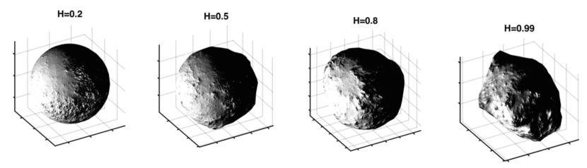
(a) Spherical simulations at 0.1° resolution for different values of $H$ ($\alpha$=1.9 and $C_{1}=0.1$). $H$ varies from 0.2 to 0.99. Synthetic bodies with low $H$ values have little large-scale altitude fluctuations and are rough at small scales. As a result, their shape is similar to a regular sphere but with a rough texture. When $H$ increases, this behavior tends to be reversed : large altitude variations appear at large scales deforming the body, which has a smoother texture.

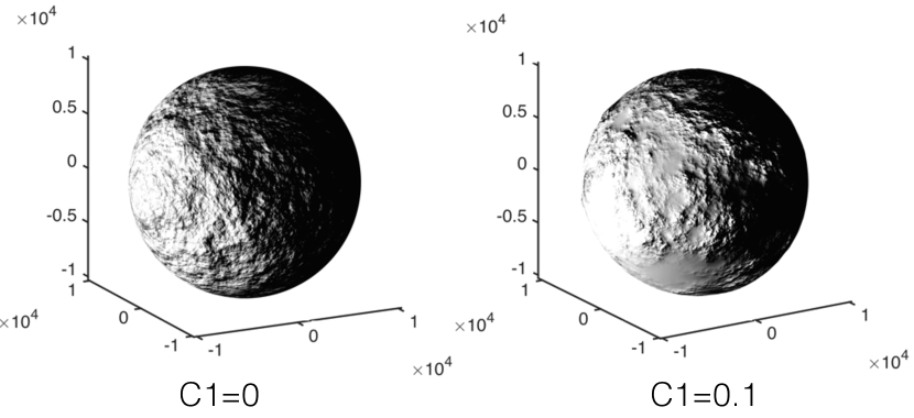
(b) Spherical simulations at 0.1° resolution for two values of $C_{1}$ ($\alpha$=1.9 and $H=0.5$ constant). From left to right $C_{1}$ is 0 and 0.1. The left simulation ($C_{1}$ = 0) is characterized by a spatially homogeneous roughness. On the contrary, themultifractal simulation on the right shows alternating smooth and rough areas

Figure 2: Several example of synthetic spherical topographic fields by varying H and $C_{1}$

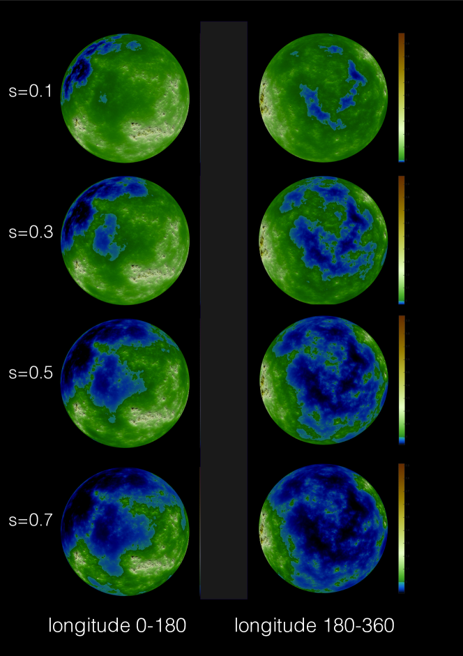
Figure 3: Synthetic multifractal topography at 0.1° resolution as a function of sea level. The fraction of the planet’s surface covered by ocean is noted s. The simulation is set for the Earth/Mars like planet ($H$ = 0.5, $\alpha$ = 1.9, $C_{1}$ = 0.1). Low altitude regions are smoother than high altitude ones. See also video 2 in sup.mat.

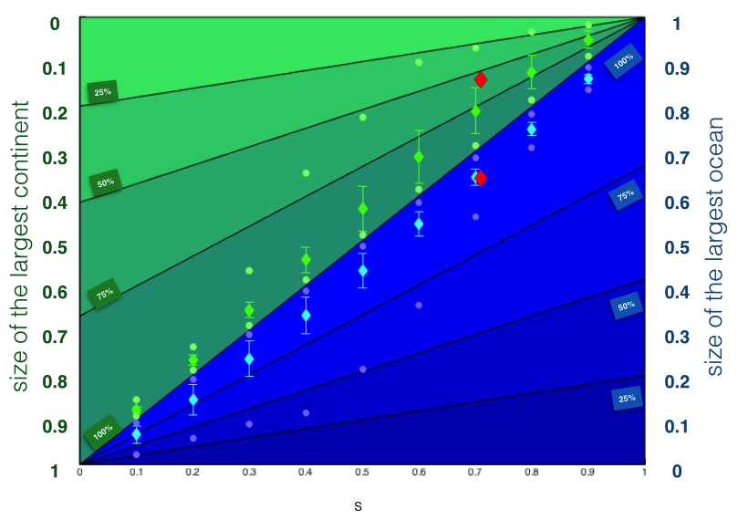
Figure 4: The Ocean/continent relationship. The size (as proportion of the total planet surface) of the largest continent (blue) and ocean (green)) for different values of sea level s. The diamond indicate the mean size with one standard deviation bars, whereas the circles indicate the minimum and maximum value in each case. The blue and green lines ) correspond to proportions of the remaining area covered by continents and ocean . These results are based on 500 synthetic topography simulations of an Earth-like planet ($H$ = 0.5, $\alpha$ = 1.9, $C_{1}$ = 0.1). The red diamonds are for the Earth.

To estimate the properties of potential exoplanet surfaces, we conducted a statistical analysis of oceans and continents obtained from 500 simulated multifractal topography fields at 1° spatial resolution with the set of parameters obtained for the global estimates on Earth ($H=0.5$, $\alpha=1.9$, $C_{1}=0.1$). In order to deal with the notion of oceans and continents, one must first define the sea/land cover. We define the sea level $s$, as a quantile of the global topographic distribution. This definition simply means that at quantile $s$, the sea level is such as $s$ is also the surface proportion of the sea. For instance, (i) $s=0.5$ is the median altitude and half of the planet is ocean covered , half by land; (ii) $s=0.9$ means that 90% of the planet area is ocean covered and 10% is land. Oceans and continents are respectively defined as disconnected areas located beneath or above the sea level $s$. We plotted on figure 3 a example of synthetic multifractal topographies with varying ratio $s$.

On Figure 4 we plotted the size of the largest continent and largest ocean as functions of $s$. We summarized the 500 experiments by computing the average, standard deviation and minimum/maximum. As one can see, the simulations produce typically one large ocean or one large continent with a size close to the maximum available area indicating that it is highly improbable to obtain two disconnected large areas. However, at respectively very small or very large values of $s$, the available area is split between several small oceans (conversely, large $s$ and small continents). Finally, we apply the same analysis on the particular case of Earth based on ETOPO1 (Amante and Eakins, 2009) and use red diamonds to indicate the size of the largest ocean and continents as functions of the terrestrial value of s ($s\approx 0.66$). The points are satisfyingly close to those obtained by multifractal simulations supporting the accuracy of the model.

Following Dohm and Maruyama (2015), we investigate the interface between ocean, atmosphere and land. From our results, on average the size of the largest ocean or continent is always close to the maximum available size (near the 90% line). The congruent part of the surface covered by ocean (or land) is split up into smaller but more numerous islands (or lakes), as also observed on the Earth (Downing et al., 2006). There are some extreme cases, where the largest continent is very small. Interestingly, this case happens more for small sea levels. If $s=0.1$, the extreme case can even reach 25%, meaning that the largest ocean only covers 25% of the ocean surface , 75% are thus covered by smaller lakes. The symmetric situation occurs for $s=0.9$ : the largest continent only covers 25% of the land, 75% are thus covered by small islands. The Earth corresponds to the average situation since all the major oceans are connected through the thermo-haline circulation. From this study, we can exclude the situation of two large unconnected oceans, representing a global sea surface > 50%. The same for two large unconnected continents, representing a global sea surface > 50%. As a summary, the interface between land and sea, so important for habitability, can be statistically constrained by this model.

4 Conclusion

Multifractal simulations on spheres are able to statistically reproduce the morphology of planetary bodies, and even potentially small bodies such asteroids and comets. In addition, it offers a wide field of investigation for evaluating the role of the topography in exoplanet signals , thanks to photometry and specular reflection, this is especially true for transiting objects . The simulations will serve as a starting point for future studies aimed at characterizing the overall photometric response of unresolved rotating bodies. Our synthetic numerical topographies can be integrated into the development of realistic exoplanet climate simulations in different contexts by integrating the roles of clouds and surface / atmosphere interactions. In particular, exoplanets in gravitational lock are subjected to climatic instabilities (Kite et al., 2011). In particular, our results suggest that it is statistically highly unlikely to have two major united oceans on either side of the globe. If the dark side is too cold and the sunny side too hot to allow the presence of liquid water, the topography could contribute to creating to a global glacier, continually moving the volatile elements from the illuminated side to the dark side. This dynamic state should significantly increase the presence of liquid water at the terminator with consequences for habitability.

By construction the statistical properties of all our simulations are isotropic. The procedure used can be modified to generate anisotropic topographies but poses a number of technical problems that have not yet been addressed. Anisotropy adds degrees of freedom that make the problem more complex both in generation but also in determining parameters on real data. To deal with this question, we should consider implementing the formalism of generalized scale invariance (GSI, Schertzer, 2011) as a future work.

We provide a 3D visualization of some examples with varying parameters (https://data.ipsl.fr/exotopo/). In addition, a dataset of synthetic spherical topographies can be downloaded by the reader (http://dx.doi.org/10.14768/20181024001.1)

References

- Amante and Eakins (2009) Amante, C., and B. Eakins (2009), Etopo1 1 arc-minute global relief model: Procedures, data sources and analysis., NOAA Technical Memorandum NESDIS NGDC-24. National Geophysical Data Center, NOAA.
- Bean et al. (2010) Bean, J. L., E. M.-R. Kempton, and D. Homeier (2010), A ground-based transmission spectrum of the super-earth exoplanet gj 1214b, Nature, 468(7324), 669–672.
- Blumsack (1971) Blumsack, S. L. (1971), On the effects of topography on planetary atmospheric circulation, Journal of the Atmospheric Sciences, 28(7), 1134–1143, doi:10.1175/1520-0469(1971)028<1134:OTEOTO>2.0.CO;2.
- Charnay et al. (2013) Charnay, B., F. Forget, R. Wordsworth, J. Leconte, E. Millour, F. Codron, and A. Spiga (2013), Exploring the faint young sun problem and the possible climates of the archean earth with a 3-D GCM, J. Geophys. Res. Atmos., 118(18), 10,414–10,431, doi:10.1002/jgrd.50808.
- de Wit et al. (2016) de Wit, J., et al. (2016), A combined transmission spectrum of the earth-sized exoplanets trappist-1 b and c, Nature, 537(7618), 69–72, doi:10.1038/nature18641.
- Demory et al. (2013) Demory, B.-O., et al. (2013), Inference of inhomogeneous clouds in an exoplanet atmosphere, The Astrophysical Journal Letters, 776(2), L25.
- Dohm and Maruyama (2015) Dohm, J. M., and S. Maruyama (2015), Habitable trinity, Geoscience Frontiers, 6(1), 95 – 101, doi:http://dx.doi.org/10.1016/j.gsf.2014.01.005, special Issue: Plate and plume tectonics: Numerical simulation and seismic tomography.
- Downing et al. (2006) Downing, J. A., et al. (2006), The global abundance and size distribution of lakes, ponds, and impoundments, Limnology and Oceanography, 51(5), 2388–2397, doi:10.4319/lo.2006.51.5.2388.
- Forget and Leconte (2014) Forget, F., and J. Leconte (2014), Possible climates on terrestrial exoplanets, Philosophical Transactions of the Royal Society of London A: Mathematical, Physical and Engineering Sciences, 372(2014), doi:10.1098/rsta.2013.0084.
- Gagnon et al. (2006) Gagnon, J.-S., S. Lovejoy, and D. Schertzer (2006), Multifractal earth topography, Nonlinear Processes in Geophysics, 13(5), 541–570, doi:10.5194/npg-13-541-2006.
- Houze (2012) Houze, R. A. (2012), Orographic effects on precipitating clouds, Reviews of Geophysics, 50(1), n/a–n/a, doi:10.1029/2011RG000365, rG1001.
- Kite et al. (2011) Kite, E. S., E. Gaidos, and M. Manga (2011), Climate instability on tidally locked exoplanets, The Astrophysical Journal, 743(1), 41.
- Landais et al. (2015) Landais, F., F. Schmidt, and S. Lovejoy (2015), Universal multifractal martian topography, Nonlinear Processes in Geophysics, 22(6), 713–722, doi:10.5194/npg-22-713-2015.
- Landais et al. (2018) Landais, F., F. Schmidt, and S. Lovejoy (2018), Multifractal topography of several planetary bodies in the solar system, Icarus, http://arxiv.org/abs/1805.11249.
- Lavallee et al. (1993) Lavallee, D., S. Lovejoy, D. Schertzer, and P. Ladoy (1993), Nonlinear variability and landscape topography: analysis and simulation. fractals in geography, Eds. L. De Cola, N. Lam, 158-192, PTR, Prentice Hall.
- Lovejoy (2014) Lovejoy, S. (2014), A voyage through scales, a missing quadrillion and why the climate is not what you expect, Climate Dynamics.
- Lovejoy and Schertzer (2007) Lovejoy, S., and D. Schertzer (2007), Scaling and multifractal fields in the solid earth and topography, Nonlinear Processes in Geophysics, 14(4), 465–502.
- Lovejoy and Schertzer (2012) Lovejoy, S., and D. Schertzer (2012), Haar wavelets, fluctuations and structure functions: convenient choices for geophysics, Nonlinear Processes in Geophysics, 19(5), 513–527, doi:10.5194/npg-19-513-2012.
- Lovejoy and Shertzer (2013) Lovejoy, S., and D. Shertzer (2013), The Weather and Climate :Emergent Laws and Multifractal Cascades, Cambridge.
- Lowry et al. (2012) Lowry, S., S. Duddy, B. Rozitis, S. F. Green, A. Fitzsimmons, C. Snodgrass, H. H. Hsieh, and O. Hainaut (2012), The nucleus of comet 67p/churyumov-gerasimenko-a new shape model and thermophysical analysis, Astronomy & Astrophysics, 548, A12.
- Mandelbrot (1967) Mandelbrot, B. (1967), How long is the coast of britain? statistical self-similarity and fractional dimension, Science, 156(3775), 636–638, doi:10.1126/science.156.3775.636.
- Mayor and Queloz (1995) Mayor, M., and D. Queloz (1995), A jupiter-mass companion to a solar-type star, Nature, 378(6555), 355–359.
- Orosei et al. (2003) Orosei, R., R. Bianchi, A. Coradini, S. Espinasse, C. Federico, A. Ferriccioni, and A. I. Gavrishin (2003), Self-affine behavior of martian topography at kilometer scale from mars orbiter laser altimeter data, Journal of Geophysical Research: Planets, 108(E4), n/a–n/a, doi:10.1029/2002JE001883.
- Rosenburg et al. (2011) Rosenburg, M. A., O. Aharonson, J. W. Head, M. A. Kreslavsky, E. Mazarico, G. A. Neumann, D. E. Smith, M. H. Torrence, and M. T. Zuber (2011), Global surface slopes and roughness of the moon from the lunar orbiter laser altimeter, Journal of Geophysical Research: Planets, 116(E2), n/a–n/a, doi:10.1029/2010JE003716.
- Schertzer and Lovejoy (1987) Schertzer, D., and S. Lovejoy (1987), Physical modeling and analysis of rain and clouds by anisotropic scaling multiplicative processes, Journal of Geophysical Research: Atmospheres, 92(D8), 9693–9714, doi:10.1029/JD092iD08p09693.
- Schertzer (2011) Schertzer, S., D. Lovejoy (2011), Multifractals, generalized scale invariance and complexity in geophysics, International Journal of Bifurcation and Chaos, 21(12), 3417–3456, doi:10.1142/S0218127411030647.
- Seager (2010) Seager, D., Sara; Deming (2010), Exoplanet atmospheres, Annual Review of Astronomy and Astrophysics, vol. 48, p.631-672.
- Smith et al. (2001) Smith, D. E., et al. (2001), Mars orbiter laser altimeter: Experiment summary after the first year of global mapping of mars, Journal of Geophysical Research: Planets, 106(E10), 23,689–23,722, doi:10.1029/2000JE001364.
- Stephan et al. (2010) Stephan, K., et al. (2010), Specular reflection on titan: liquids in kraken mare, Geophysical Research Letters, 37(7).
- Tian (2015) Tian, F. (2015), Observations of exoplanets in time-evolving habitable zones of pre-main-sequence m dwarfs, Icarus, 258, 50 – 53, doi:http://dx.doi.org/10.1016/j.icarus.2015.06.004.
- Wang et al. (2014) Wang, Y., F. Tian, and Y. Hu (2014), Climate patterns of habitable exoplanets in eccentric orbits around m dwarfs, The Astrophysical Journal Letters, 791(1), L12.
- Wilson et al. (1991) Wilson, J., D. Schertzer, and S. Lovejoy (1991), Continuous Multiplicative Cascade Models of Rain and Clouds, pp. 185–207, Springer Netherlands, Dordrecht.
- Wordsworth et al. (2011) Wordsworth, R. D., F. Forget, F. Selsis, E. Millour, B. Charnay, and J.-B. Madeleine (2011), Gliese 581d is the first discovered terrestrial-mass exoplanet in the habitable zone, The Astrophysical Journal Letters, 733(2), L48.