ProBO: Versatile Bayesian Optimization Using Any Probabilistic Programming Language

Abstract.

Optimizing an expensive-to-query function is a common task in science and engineering, where it is beneficial to keep the number of queries to a minimum. A popular strategy is Bayesian optimization (BO), which leverages probabilistic models for this task. Most BO today uses Gaussian processes (GPs), or a few other surrogate models. However, there is a broad set of Bayesian modeling techniques that could be used to capture complex systems and reduce the number of queries in BO. Probabilistic programming languages (PPLs) are modern tools that allow for flexible model definition, prior specification, model composition, and automatic inference. In this paper, we develop ProBO, a BO procedure that uses only standard operations common to most PPLs. This allows a user to drop in a model built with an arbitrary PPL and use it directly in BO. We describe acquisition functions for ProBO, and strategies for efficiently optimizing these functions given complex models or costly inference procedures. Using existing PPLs, we implement new models to aid in a few challenging optimization settings, and demonstrate these on model hyperparameter and architecture search tasks.

1. Introduction

Bayesian optimization (BO) is a popular method for zeroth-order optimization of an unknown (“black box”) system. A BO procedure iteratively queries the system to yield a set of input/output data points, computes the posterior of a Bayesian model given these data, and optimizes an acquisition function defined on this posterior in order to determine the next point to query.

BO involves performing inference and optimization to choose each point to query, which can incur a greater computational cost than simpler stategies, but may be ultimately beneficial in settings where queries are expensive. Specifically, if BO can reach a good optimization objective in fewer iterations than simpler methods, it may be effective in cases where the expense of queries far outweighs the extra cost of BO. Some examples of this are in science and engineering, where a query could involve synthesizing and measuring the properties of a material, collecting metrics from an industrial process, or training a large machine learning model, which can be expensive in cost, time, or human labor.

The most common model used in BO is the Gaussian process (GP), for which we can compute many popular acquisition functions. There has also been some work deriving BO procedures for other flexible models including random forests [21] and neural networks [45]. In this paper, we argue that more-sophisticated models that better capture the details of a system can help reduce the number of iterations needed in BO, and allow for BO to be effectively used in custom and complex settings. For example, systems may have complex noise [42, 22], yield multiple types of observations [12], depend on covariates [25], have interrelated subsystems [47], and more. To accurately capture these systems, we may want to design custom models using a broader library of Bayesian tools and techniques. For example, we may want to compose models—such as GPs, latent factor (e.g. mixture) models, deep Bayesian networks, hierarchical regression models—in various ways, and use them in BO.

Probabilistic programming languages (PPLs) are modern tools for specifying Bayesian models and performing inference. They allow for easy incorporation of prior knowledge and model structure, composition of models, quick deployment, and automatic inference, often in the form of samples from or variational approximations to a posterior distribution. PPLs may be used to specify and run inference in a variety of models, such as graphical models, GPs, deep Bayesian models, hierarchical models, and implicit (simulator-based) models, to name a few [7, 30, 40, 50, 5, 33, 2, 31, 54, 9].

We would like to be able to build an arbitrary model with any PPL and then automatically carry out BO with this model. However, this comes with a few challenges. In BO with GPs, we have the posterior in closed-form, and use this when computing and optimizing acquisition functions. PPLs, however, use a variety of approximate inference procedures, which can be costly to run and yield different posterior representations (e.g. samples [7, 54], variational approximations [50, 5], implicit models [20, 51], or amortized distributions [39, 28]). We need a method that can compute and optimize acquisition functions automatically, given the variety of representations, and efficiently, making judicious use of PPL procedures.

Towards this end, we develop ProBO, a BO system for PPL models, which computes and optimizes acquisition functions via operations that can be implemented in a broad variety of PPLs. This system comprises algorithms that cache and use these operations efficiently, which allows it to be used in practice given complex models and expensive inference procedures. The overall goal of ProBO is to allow a custom model written in an arbitrary PPL to be “dropped in” and immediately used in BO.

This paper has two main contributions: (1) We present ProBO, a system for versatile Bayesian optimization using models from any PPL. (2) We describe optimization settings that are difficult for standard BO methods and models, and then use PPLs to implement new models for these settings, which are dropped into ProBO and show good optimization performance. Our open source release of ProBO is available at https://github.com/willieneis/ProBO.

2. Related Work

A few prior works make connections between PPLs and BO. BOPP [37] describes a BO method for marginal maximum a posteriori (MMAP) estimates of latent variables in a probabilistic program. This work relates BO and PPLs, but differs from us in that the goal of BOPP is to use BO (with GP models) to help estimate latent variables in a given PPL, while we focus on using PPLs to build new surrogate models for BO.

BOAT [8] provides a custom PPL involving composed Gaussian process models with parametric mean functions, for use in BO. For these models, exact inference can be performed and the expected improvement acquisition directly used. This work has similar goals as us, though we instead aim to provide a system that can be applied to models from any existing PPL (not constrained to a certain family of GP models), and specifically with PPLs that use approximate inference algorithms where we cannot compute acquisition functions in standard ways. ProBO We first describe a general abstraction for PPLs, and use this abstraction to define ProBO and present algorithms for computing a few acquisition functions. We then show how to efficiently optimize these acquisition functions.

2.1. Abstraction for Probabilistic Programs

Suppose we are modeling a system which, given an input $x\in\mathcal{X}$, yields observations $y\in\mathcal{Y}$, written $y\sim s(x)$. Let $f:\mathcal{Y}\rightarrow\mathbb{R}$ be an objective function that maps observations $y$ to real values. Observing the system $n$ times at different inputs yields a dataset $\mathcal{D}_{n}=\{(x_{i},y_{i})\}_{i=1}^{n}$. Suppose we have a Bayesian model for $\mathcal{D}_{n}$, with likelihood $p(\mathcal{D}_{n}|z)$ $=$ $\prod_{i=1}^{n}p(y_{i}|z;x_{i})$, where $z\in\mathcal{Z}$ are latent variables. We define the joint model PDF to be $p(\mathcal{D}_{n},z)=p(z)p(\mathcal{D}_{n}|z)$, where $p(z)$ is the PDF of the prior on $z$. The posterior PDF is then $p(z|\mathcal{D}_{n})=p(\mathcal{D}_{n},z)/\int p(\mathcal{D}_{n},z)dz$.

Our abstraction assumes three basic PPL operations:

1. $\texttt{inf}(\mathcal{D})$: given data $\mathcal{D}$, this runs an inference algorithm and returns an object post, which is a PPL-dependent representation of the posterior distribution.

2. $\texttt{post}(s)$: given a seed $s\in\mathbb{Z}^{+}$, this returns a sample from the posterior distribution.

3. $\texttt{gen}(x,z,s)$: given an input $x\in\mathcal{X}$, a latent variable $z\in\mathcal{Z}$, and a seed $s\in\mathbb{Z}^{+}$, this returns a sample from the generative distribution $p(y|z;x)$.

Note that post and gen are deterministic, i.e. for a fixed seed $s$, post/gen produce the same output each time they are called.

(a)   $a_{\text{EI}}(x)$ (b)   $a_{\text{PI}}(x)$ (c)   $a_{\text{UCB}}(x)$ (d)   $a_{\text{TS}}(x)$

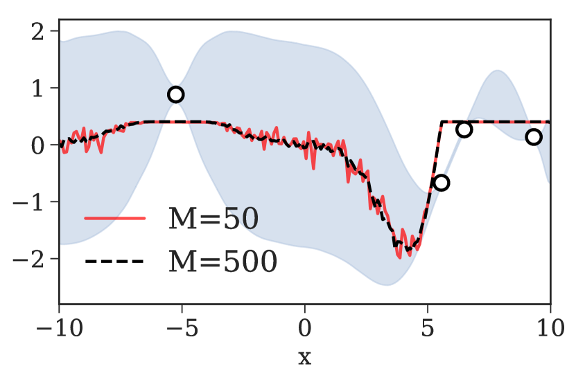
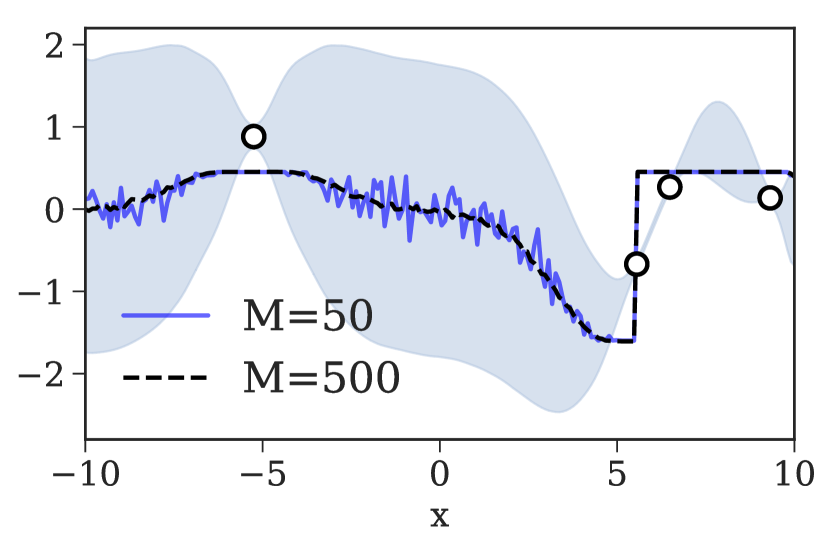
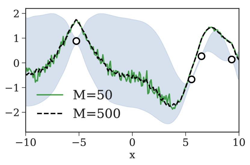
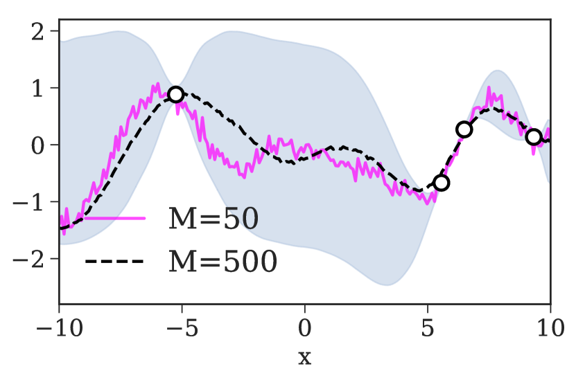
Figure 1. Visualizations of PPL acquisition functions $a(x)$ given in Algs. 2-5 for use in ProBO. In each plot, the data and posterior predictive distribution are shown, and $a(x)$ is given for two fidelities: $M=50$ (solid color line) and $M=500$ (dashed black line).

Scope.

This abstraction applies to a number of PPLs, which use a variety of inference strategies and compute different representations for the posterior. For example, in PPLs using Markov chain Monte Carlo (MCMC) or sequential Monte Carlo (SMC) algorithms [7, 40, 54], inf computes a set of posterior samples and post draws uniformly from this set. For PPLs using variational inference (VI), implicit models, or exact inference methods [50, 5, 14], inf computes the parameters of a distribution, and post draws a sample from this distribution. In amortized or compiled inference methods [39, 28, 24], inf trains or calls a pretrained model that maps observations to a posterior or proposal distribution, and post samples from this.

2.2. Main Procedure

Recall that we use PPLs to model a system $s$, which yields observations $y\sim s(x)$ given a query $x$, and where $f(y):\mathcal{Y}\rightarrow\mathbb{R}$ denotes the objective value that we want to optimize. The goal of ProBO is to return $x^{*}=\operatorname*{argmin}_{x\in\mathcal{X}}\mathbb{E}_{y\sim s(x)}\left[f(y)\right]$. We give ProBO in Alg. 1. Each iteration consists of four steps: call an inference procedure inf, select an input $x$ by optimizing an acquisition function $a$ that calls post and gen, observe the system at $x$, and add new observations to the dataset.

Algorithm 1 ProBO$\left(\mathcal{D}_{0},\texttt{inf},\texttt{gen}\right)$

1:for $n=1,\ldots,N$ do

2:     $\texttt{post}\leftarrow\texttt{inf}(\mathcal{D}_{n-1})$ $\triangleright$ Run inference algorithm to compute post

3:     $x_{n}\leftarrow\operatorname*{argmin}_{x\in\mathcal{X}}a(x,\texttt{post},\texttt{gen})$ $\triangleright$ Optimize acquisition using post and gen

4:     $y_{n}\sim s(x_{n})$ $\triangleright$ Observe system at $x_{n}$

5:     $\mathcal{D}_{n}\leftarrow\mathcal{D}_{n-1}\cup(x_{n},y_{n})$ $\triangleright$ Add new observations to dataset

6:Return $\mathcal{D}_{N}$.

Note that acquisition optimization (line 3) involves only post and gen, while inf is called separately beforehand. We discuss the computational benefits of this, and the cost of ProBO, in more detail in Sec. 2.4. Also note that many systems can have extra observations $y\in\mathcal{Y}$, in addition to the objective value, that provide information which aids optimization [55, 3, 47]. For this reason, our formalism explicitly separates system observations $y$ from their objective values $f(y)$. We show examples of models that take advantage of extra observations in Sec. 3.

In the following sections, we develop algorithms for computing acquisition functions $a(x)$ automatically using only post and gen operations, without requiring any model specific derivation. We refer to these as PPL acquisition functions.

2.3. PPL Acquisition Functions via post and gen

In ProBO (Alg. 1), we denote the PPL acquisition function with $a(x,\texttt{post},\texttt{gen})$. Each PPL acquisition algorithm includes a parameter $M$, which represents the fidelity of the approximation quality of $a$. We will describe an adaptive method for choosing $M$ during acquisition optimization in Sec. 2.5. Below, we will make use of the posterior predictive distribution, which is defined to be $p(y|\mathcal{D}_{n};x)$ $=$ $\mathbb{E}_{p(z|\mathcal{D}_{n})}\left[p(y|z;x)\right]$.

There are a number of popular acquisition functions used commonly in Bayesian optimization, such as expected improvement (EI) [34], probability of improvement (PI) [26], GP upper confidence bound (UCB) [46], and Thompson sampling (TS) [48]. Here, we propose a few simple acquisition estimates that can be computed with post and gen. Specifically, we give algorithms for EI (Alg. 2), PI (Alg. 3), UCB (Alg. 4), and TS (Alg. 5) acquistion strategies, though similar algorithms could be used for other acquisitions involving expectations or statistics of either $p(y|D_{n};x)$ or $p(y|z;x)$.

We now describe the PPL acquisition functions given in Alg. 2-5 in more detail, and discuss the approximations given by each. Namely, we show that these yield versions of exact acquisition functions as $M\rightarrow\infty$. These algorithms are related to Monte Carlo acquisition function estimates for GP models [44, 15, 16], which have been developed for specific acquisition functions.

Expected Improvement (EI), Alg. 2

Let $\mathcal{D}$ be the data at a given iteration of ProBO. In our setting, the expected improvement (EI) acquisition function will return the expected improvement that querying the system at $x\in\mathcal{X}$ will have over the minimal observed objective value, $f_{\text{min}}=\min_{y\in\mathcal{D}}f(y)$. We can write the exact EI acquisition function as

$$a_{\text{EI}}^{*}(x)=\int\mathds{1}\left\{f(y)\leq f_{\text{min}}\right\}\left(f_{\text{min}}-f(y)\right)p\left(y|\mathcal{D};x\right)dy.$$ (2.1)

In Alg. 2, for a sequence of steps $m=1,\ldots,M$, we draw $z_{m}\sim p(z|\mathcal{D})$ and $y_{m}\sim p(y|z_{m};x)$ via post and gen, and then compute $\lambda(y_{1:M})=\sum_{m=1}^{M}\mathds{1}\left[f(y_{m})\leq f_{\text{min}}\right](f_{\text{min}}-f(y_{m}))$. Marginally, $y_{m}$ is drawn from the posterior predictive distribution, i.e. $y_{m}$ $\sim$ $\mathbb{E}_{p(z|\mathcal{D})}\left[p(y|z;x)\right]$ $=$ $p(y|\mathcal{D};x)$. Therefore, as the number of calls $M$ to post and gen grows, $a_{\text{EI}}(x)$ $\rightarrow$ $a_{\text{EI}}^{*}(x)$ (up to a multiplicative constant) at a rate of $O(\sqrt{M})$.

Algorithm 2  $a_{\text{EI}}\left(x,\texttt{post},\texttt{gen}\right)$ $\triangleright$ EI

1:for $m=1,\ldots,M$ do

2:     $z_{m}\leftarrow\texttt{post}(s_{m})$

3:     $y_{m}\leftarrow\texttt{gen}(x,z_{m},s_{m})$

4:$f_{\text{min}}\leftarrow\min_{y\in\mathcal{D}}f(y)$

5:Return $\sum_{m=1}^{M}\mathds{1}\left[f(y_{m})\leq f_{\text{min}}\right](f_{\text{min}}-f(y_{m}))$

Algorithm 3  $a_{\text{PI}}\left(x,\texttt{post},\texttt{gen}\right)$ $\triangleright$ PI

1:for $m=1,\ldots,M$ do

2:     $z_{m}\leftarrow\texttt{post}(s_{m})$

3:     $y_{m}\leftarrow\texttt{gen}(x,z_{m},s_{m})$

4:$f_{\text{min}}\leftarrow\min_{y\in\mathcal{D}}f(y)$

5:Return $\sum_{m=1}^{M}\mathds{1}\left[f(y_{m})\leq f_{\text{min}}\right]$

Algorithm 4  $a_{\text{UCB}}\left(x,\texttt{post},\texttt{gen}\right)$ $\triangleright$ UCB

1:for $m=1,\ldots,M$ do

2:     $z_{m}\leftarrow\texttt{post}(s_{m})$

3:     $y_{m}\leftarrow\texttt{gen}(x,z_{m},s_{m})$

4:Return $\widehat{\text{LCB}}\left(f(y_{m})_{m=1}^{M}\right)$ $\triangleright$ See text for details

Algorithm 5  $a_{\text{TS}}\left(x,\texttt{post},\texttt{gen}\right)$ $\triangleright$ TS

1:$z\leftarrow\texttt{post}(s_{1})$

2:for $m=1,\ldots,M$ do

3:     $y_{m}\leftarrow\texttt{gen}(x,z,s_{m})$

4:Return $\sum_{m=1}^{M}f(y_{m})$

Probability of Improvement (PI), Alg. 3

In our setting, the probability of improvement (PI) acquisition function will return the probability that observing the system at query $x\in\mathcal{X}$ will improve upon the minimally observed objective value, $f_{\text{min}}=\min_{y\in\mathcal{D}}f(y)$. We can write the exact PI acquisition function as

$$a_{\text{PI}}^{*}(x)=\int\mathds{1}\left\{f(y)\leq f_{\text{min}}\right\}p\left(y|\mathcal{D};x\right)dy.$$ (2.2)

In Alg. 3, for a sequence of steps $m=1,\ldots,M$, we draw $z_{m}\sim p(z|\mathcal{D})$, $y_{m}\sim p(y|z_{m};x)$ via post and gen, and then compute $\lambda(y_{1:M})=\sum_{m=1}^{M}\mathds{1}\left[f(y_{m})\leq f_{\text{min}}\right]$. As before, $y_{m}$ is drawn (marginally) from the posterior predictive distribution. Therefore, as the number of calls $M$ to post and gen grows, $a_{\text{PI}}(x)$ $\rightarrow$ $a_{\text{PI}}^{*}(x)$ (up to a multiplicative constant) at a rate of $O(\sqrt{M})$.

Upper Confident Bound (UCB), Alg. 4

We propose an algorithm based on the principle of optimization under uncertainty (OUU), which aims to compute a lower confidence bound for $p(f(y)|\mathcal{D};x)$, which we denote by $\text{LCB}\left[p(f(y)|\mathcal{D}_{n};x)\right]$. In Alg. 4, we use an estimate of this, $\widehat{\text{LCB}}(f(y_{m})_{m=1}^{M})$. Note that we use a lower confidence bound since we are performing minimization, though we denote our acquisition function with the more commonly used title UCB. Two simples strategies for estimating this LCB are

1. Empirical quantiles: Order $f(y_{m})_{m=1}^{M}$ into $f_{(1)}\leq\ldots\leq f_{(M)}$, and return $f_{(b)}$ if $b\in\mathbb{Z}$, or else return $\frac{1}{2}(f_{(\lfloor b\rfloor)}+f_{(\lfloor b\rfloor+1)})$, where $b\in[0,M+1]$ is a tradeoff parameter.

2. Parametric assumption: As an example, if we model $p(f(y)|\mathcal{D}_{n};x)$ $=$ $\mathcal{N}(f(y)|\mu,\sigma^{2})$, we can compute $\hat{\mu}$ $=$ $\frac{1}{M}\sum_{m=1}^{M}f(y_{m})$ and $\hat{\sigma}^{2}$ $=$ $\frac{1}{M-1}\sum_{m=1}^{M}(f(y_{m})-\hat{\mu})^{2}$, and return $\hat{\mu}-\beta\hat{\sigma}^{2}$, where $\beta>0$ is a trade-off parameter.

The first proposed estimate (empirical quantiles) is a consistent estimator, though may yield worse performance in practice than the second proposed estimate in cases where we can approximate $p(f(y_{m})|\mathcal{D};x)$ with some parametric form.

Thompson Sampling (TS), Alg. 5

Thompson sampling (TS) proposes proxy values for unknown model variables by drawing a posterior sample, and then performs optimization as if this sample were the true model variables, and returns the result. In Alg. 5, we provide an acquisition function to carry out a TS strategy in ProBO , using post and gen. At one given iteration of BO, a specified seed is used so that each call to $a_{\text{TS}}(x)$ produces the same posterior latent variable sample $\tilde{z}\sim p(z|\mathcal{D})$ via post. After, gen is called repeatedly to produce $y_{m}\sim p(y|\tilde{z};x)$ for $m=1,\ldots,M$, and the objective values of these are averaged to yield $\lambda(y_{1:M})=\sum_{m=1}^{M}f(y_{m})$. Here, each $f(y_{m})\sim\mathbb{E}_{p(y|\tilde{z};x)}\left[f(y)\right]$. Optimizing this acquisition function serves as a proxy for optimizing our model given the true model variables, using posterior sample $\tilde{z}$ in place of unknown model variables.

In Summary

As $M\rightarrow\infty$, for constants $c_{1}$, $c_{2}$, $c_{3}$, and $c_{4}$,

$$a_{\text{EI}}(x,\texttt{post},\texttt{gen}) \rightarrow c_{1}\int\mathds{1}\left\{f(y)\leq\min_{y^{\prime}\in\mathcal{D}}f(y^{\prime})\right\}\left(\min_{y^{\prime}\in\mathcal{D}}f(y^{\prime})-f(y)\right)p(y|\mathcal{D};x)dy$$ (2.3)

$$a_{\text{PI}}(x,\texttt{post},\texttt{gen}) \rightarrow c_{2}\int\mathds{1}\left\{f(y)\leq\min_{y^{\prime}\in\mathcal{D}}f(y^{\prime})\right\}p(y|\mathcal{D};x)dy$$ (2.4)

$$a_{\text{UCB}}(x,\texttt{post},\texttt{gen}) \rightarrow c_{3}\hskip 2.84526pt\text{LCB}\left[p(f(y)|\mathcal{D};x)\right]$$ (2.5)

$$a_{\text{TS}}(x,\texttt{post},\texttt{gen}) \rightarrow c_{4}\int f(y)\hskip 2.84526ptp(y|\tilde{z};x)dy,\hskip 5.69054pt\text{ for }\tilde{z}\sim p(z|\mathcal{D}),$$ (2.6)

We visualize Alg. 2-5 in Fig. 1 (a)-(d), showing $M\in\{50,500\}$.

2.4. Computational Considerations

In ProBO, we run a PPL’s inference procedure when we call inf, which has a cost dependent on the underlying inference algorithm. For example, most MCMC methods have complexity $O(n)$ per iteration [4]. However, ProBO only runs inf once per query; acquisition optimization, which may be run hundreds of times per query, instead uses only post and gen. For many PPL models, post and gen can be implemented cheaply. For example, post often involves drawing from a pool of samples or from a known distribution, and gen often involves sampling from a fixed-length sequence of known distributions and transformations, both of which typically have $O(1)$ complexity. However, for some models, gen can involve running a more costly simulation. For these cases, we provide acquisition optimization algorithms that use post and gen efficiently in Sec. 2.5.

2.5. Efficient Optimization of PPL Acquisition Functions

In ProBO, we must optimize over the acquisition algorithms defined in the previous section, i.e. compute $x_{n}=\operatorname*{argmin}_{x\in\mathcal{X}}a(x,\texttt{post},\texttt{gen})$. Note that post and gen are not in general analytically differentiable, so in contrast with [53], we cannot optimize $a(x)$ with gradient-based methods. We therefore explore strategies for efficient zeroth-order optimization.

In Alg. 2-5, $M$ denotes the number of times post and gen are called in an evaluation of $a(x)$. As seen in Fig. 1, a small $M$ will return a noisy estimate of $a(x)$, while a large $M$ will return a more-accurate estimate. However, for some PPLs, the post and/or gen operations can be costly (e.g. if gen involves a complex simulation [49, 32]), and we’d like to minimize the number of times they are called.

This is a special case of a multi-fidelty optimization problem [11], with fidelity parameter $M$. Unlike typical multi-fidelity settings, our goal is to reduce the number of calls to post and gen for a single $x$ only, via modifying the acquisition function $a(x,\texttt{post},\texttt{gen})$. This way, we can drop in any off-the-shelf optimizer that makes calls to $a$. Suppose we have $F$ fidelities ranging from a small number of samples $M_{\text{min}}$ to a large number $M_{\text{max}}$, i.e. $M_{\text{min}}=M_{1}<\ldots<M_{F}=M_{\text{max}}$. Intuitively, when calling $a(x,\texttt{post},\texttt{gen})$ on a given $x$, we’d like to use a small $M$ if $a(x)$ is far from the minimal value $a(x^{*})$, and a larger $M$ if $a(x)$ is close to $a(x^{*})$.

We propose the following procedure: Suppose $a_{\text{min}}$ is the minimum value of $a$ seen so far during optimization (for any $x$). For a given fidelity $M_{f}$ (starting with $f$$=$$1$), we compute a lower confidence bound (LCB) for the sampling distribution of $a(x,\texttt{post},\texttt{gen})$ with $M_{f}$ calls to post and gen. We can do this via the bootstrap method [10] along with the LCB estimates described in Sec. 2.3. If this LCB is below $a_{\text{min}}$, it remains plausible that the acquisition function minimum is at $x$, and we repeat these steps at fidelity $M_{f+1}$. After reaching a fidelity $f^{*}$ where the LCB is above $a_{\text{min}}$ (or upon reaching the highest fidelity $f^{*}=F$), we return the estimate $a(x,\texttt{post},\texttt{gen})$ with $M_{f^{*}}$ calls. We give this procedure in Alg. 6.

Algorithm 6  $a_{\text{MF}}\left(x,\texttt{post},\texttt{gen}\right)$

1:$a_{\text{min}}\leftarrow$ Min value of $a$ seen so far

2:$\ell=-\infty$, $f=1$

3:while $\ell\leq a_{\text{min}}$ do

4:     $\ell\leftarrow\text{LCB-bootstrap}\left(\texttt{post},\texttt{gen},M_{f}\right)$

5:     $f\leftarrow f+1$

6:Return $a(x,\texttt{post},\texttt{gen})$ using $M=M_{f}$

Algorithm 7   LCB-bootstrap$(\texttt{post},\texttt{gen},M_{f})$

1:$y_{1:M_{f}}\leftarrow$ Call post and gen $M_{f}$ times

2:for $j=1,\ldots,B$ do

3:     $\tilde{y}_{1:M_{f}}\leftarrow$ Resample$(y_{1:M_{f}})$

4:     $a_{j}\leftarrow\lambda(\tilde{y}_{1:M_{f}})$ $\triangleright$ See text for details

5:Return $\text{LCB}\left(a_{1:B}\right)$

In Alg. 7 we use notation $\lambda(y_{1:M})$ to denote the final operation (last line) in one of Algs. 2-5 (e.g. $\lambda_{a}(y_{1:M})$ $=$ $\sum_{m=1}^{M}\mathds{1}[f(y_{m})\leq f_{\text{min}}]$ in the case of PI). As a simple example, we could run a two-fidelity algorithm, with $M\in\{M_{1},M_{2}\}$, where $M_{1}\ll M_{2}$. For a given $x$, $a_{\text{MF}}$ would first call post and gen $M_{1}$ times, and compute the LCB with the bootstrap. If the LCB is greater than $a_{\text{min}}$, it would return an $a(x,\texttt{post},\texttt{gen})$ with the $M_{1}$ calls; if not, it would return it with $M_{2}$ calls. Near optima, this will make $M_{1}+M_{2}$ calls to post and gen, and will make $M_{1}$ calls otherwise.

One can apply any derivative-free (zeroth-order) global optimization procedure that iteratively calls $a_{\text{MF}}$. In general, we can replace the optimization step in ProBO (Alg. 1, line 3) with $x_{n}\leftarrow\operatorname*{argmin}_{x\in\mathcal{X}}a_{\text{MF}}(x)$, for each of the PPL acquisition functions described in Sec. 2.3. In Sec. 3.5, we provide experimental results for this method, showing favorable performance relative to high fidelity acquisition functions, as well as reduced calls to post and gen.

3. Examples and Experiments

We provide examples of models to aid in complex optimization scenarios, implement these models with PPLs, and show empirical results. Our main goals are to demonstrate that we can plug models built with various PPLs into ProBO, and use these to improve BO performance (i.e. reduce the number of iterations) when compared with standard methods and models. We also aim to verify that our acquisition functions and extensions (e.g. multi-fidelity $a_{\text{MF}}$) perform well in practice.

PPL Implementations:

We implement models with Stan [7] and Edward [50], which (respectively) make use of the No U-Turn Sampler [18] (a form of Hamiltonian Monte Carlo) and black box variational inference [38]. We also use George [2] and GPy [14] for GP comparisons.

3.1. BO with State Observations

Setting:

Some systems exhibit unique behavior in different regions of the input space $\mathcal{X}$ based on some underlying state. We often do not know these state regions apriori, but can observe the state of an $x$ when it is queried. Two examples of this, for computational systems, are:

• Timeouts or failures: there may be regions where queries fail or time out. We can observe if a query has a “pass” or “fail” state [12, 13, 27].

• Resource usage regions: queries can have distinct resource usage patterns. We can observe this pattern for a query, and use it to assign a state [1, 8].

Assume that for each query $x\in\mathcal{X}$, $s(x)$ returns a $y\in\mathcal{Y}=\mathbb{R}\times\mathbb{Z}^{+}$, with two types of information: an objective value $y_{0}$ and an state observation $y_{1}$ indicating the region assignment. We take the objective function to be $f(y)=y_{0}$.

Model:

Instead of using a single black box model for the entire input space $\mathcal{X}$ we provide a model that infers the distinct regions and learns a model for each. For the case of two states, we can write the generative model for this as: $c\sim\text{Bernoulli}(\cdot|C(x))$, $y\sim cM_{1}(\cdot|x)+(1-c)M_{2}(\cdot|x)$, where $M_{1}$ and $M_{2}$ are models for $y|x$ (e.g. GP regression models) and $C$ is a classification model (e.g. a Bayesian NN) that models the probability of $M_{1}$. We refer to this model as a switching model. This model could be extended to more states. We show inference in this model in Fig. 2 (d). Comparing this with a a GP (Fig. 2 (c)), we see that GP hyperparameter estimates can be negatively impacted due to the nonsmooth landscape around region boundaries.

Empirical Results:

We demonstrate the switching model on the task of neural network architecture and hyperparameter search [56, 23] with timeouts, where in each query we train a network and return accuracy on a held out validation set. However, training must finish within a given time threshold, or it times out, and instead returns a preset (low accuracy) value. We optimize over multi-layer perceptron (MLP) neural networks, where we represent each query as a vector $x\in\mathbb{R}^{4}$, where $x$ = $($number of layers, layer width, learning rate, and batch size$)$. We train and validate each network on the Pima Indians Diabetes Dataset [43]. Whenever training has not converged within 60 seconds, the system times out and returns a fixed accuracy value of $30\%$. We use a GP regression model for $M_{1}$, and a Gaussian model (with mean and variance latent variables) for $M_{2}$. We compare ProBO with this switching model against standard BO using GPs, plotting the maximum validation accuracy found vs iteration $n$, averaged over 10 trials, in Fig. 2 (e)-(f).

BO with State Observations

(a) Data and true system mean

(b) GP (on state 1 data only)

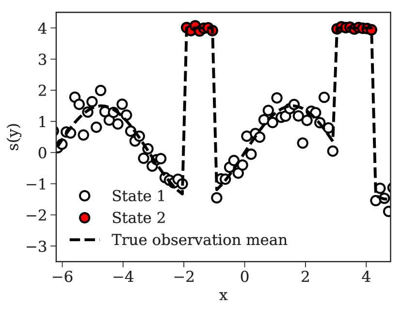
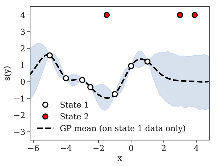
(c) GP (on all data)

(d) Switching model (on all data)

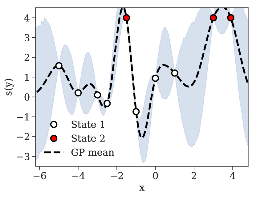
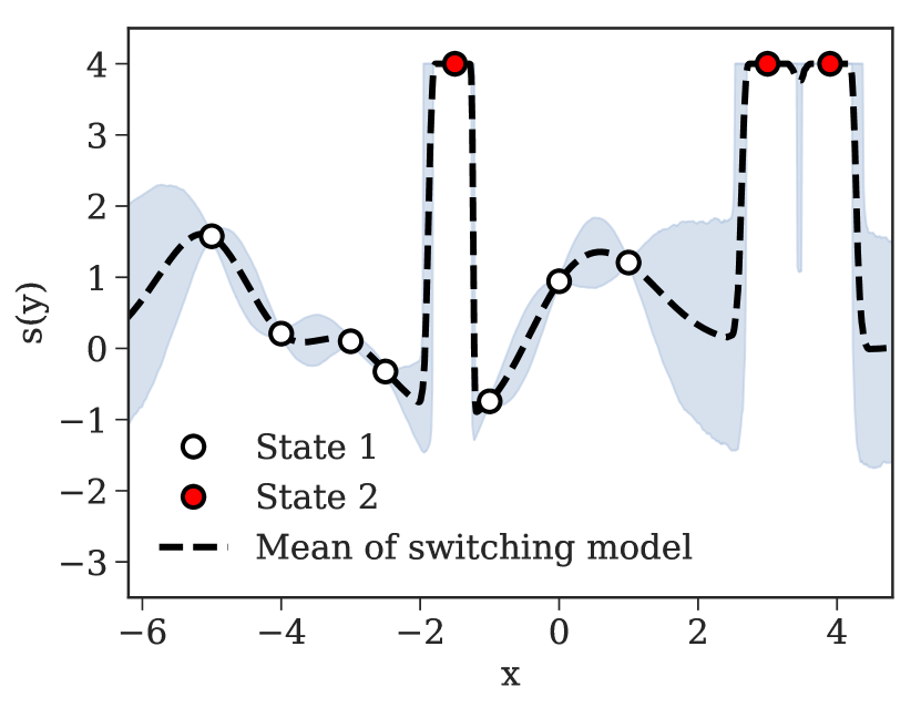
(e) EI and UCB

(f) PI and TS

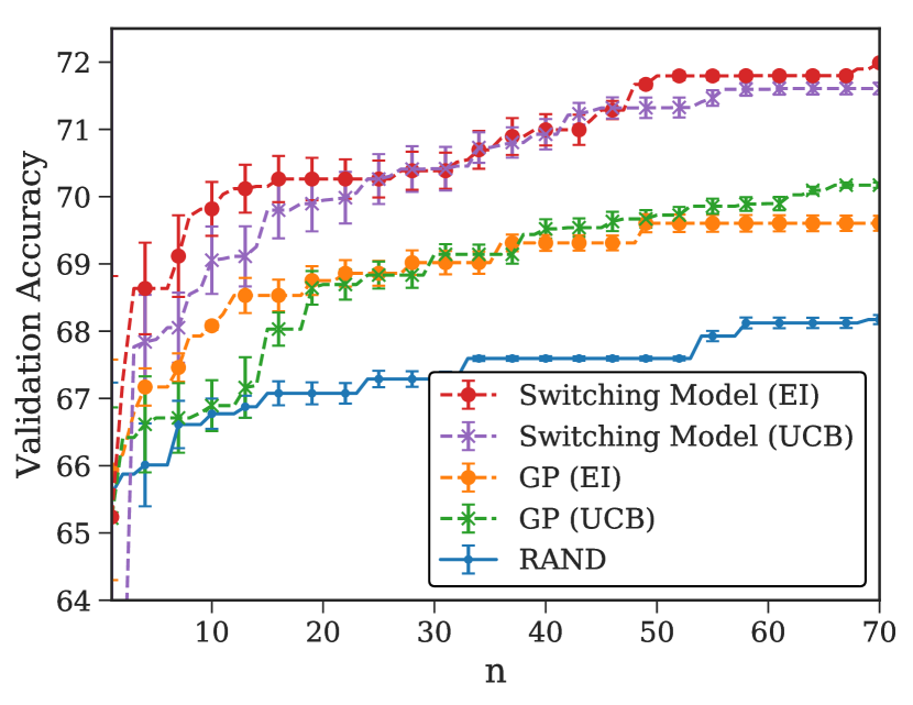
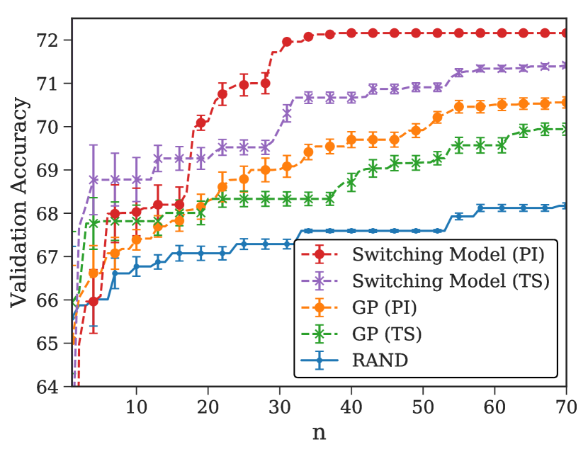
Figure 2. BO with state observations (Sec. 3.1). We show (a) the true system, and inference results on (b) a GP model fit on state 1 data only, (c) the same GP model fit on all data, where hyperparameter estimates are badly influenced, and (d) our switching model fit on all data. In (e)-(f) we show results on the task of neural network architecture and hyperparameter search with timeouts, comparing ProBO using a switching model to BO using GPs. Curves are averaged over 10 trials, and error bars represent one standard error.

Contaminated BO

(a) GP ($n=20$)

(b) GP ($n=50$)

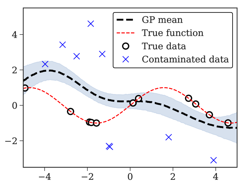
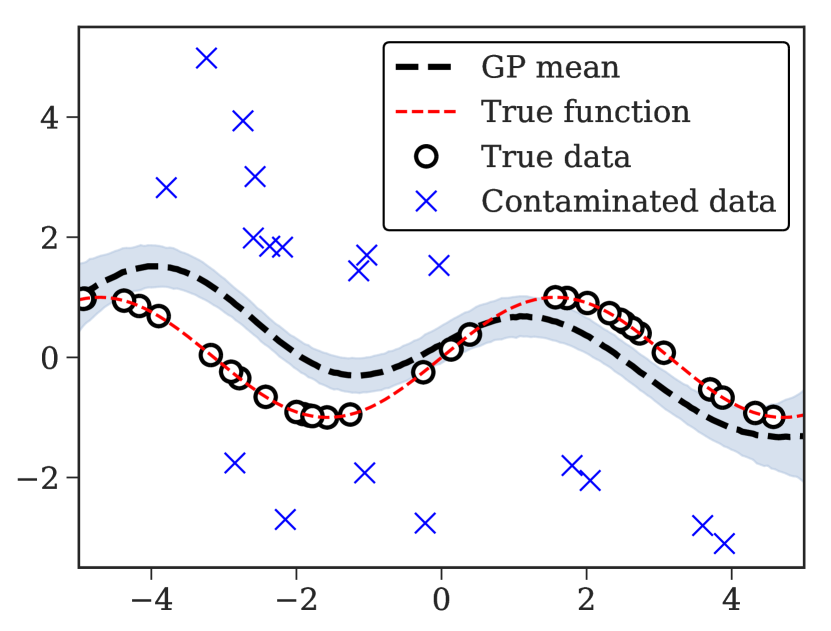
(c) Denoising GP ($n=20$)

(d) Denoising GP ($n=50$)

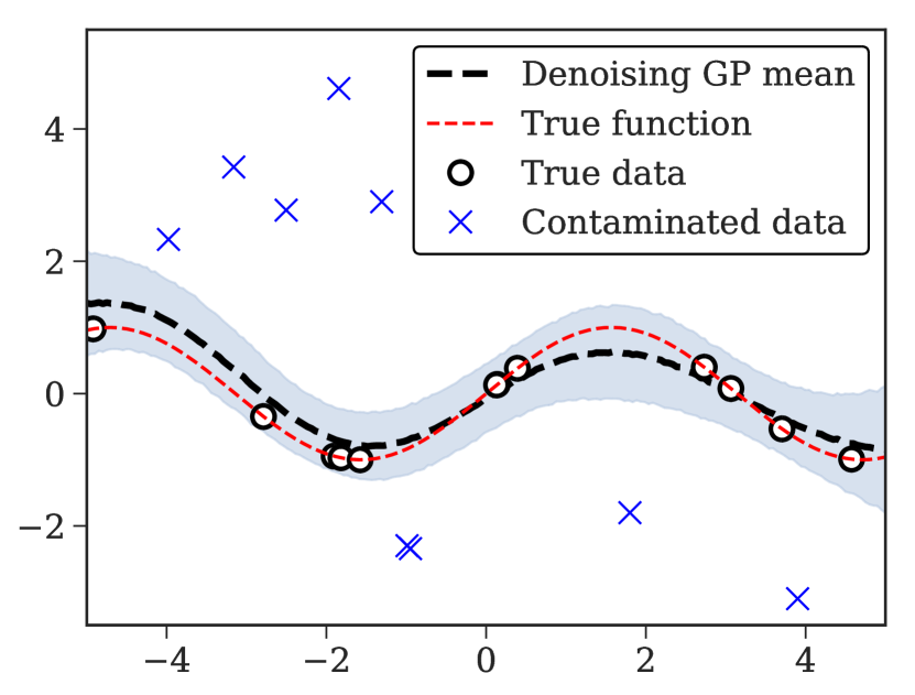
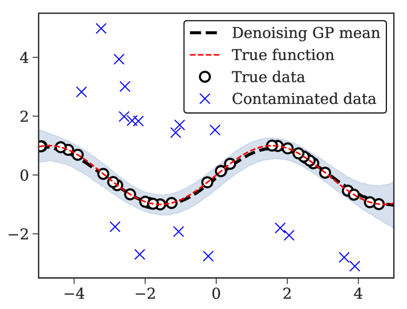
(e) EI and UCB ($p=.01$)

(f) PI and TS ($p=.01$)

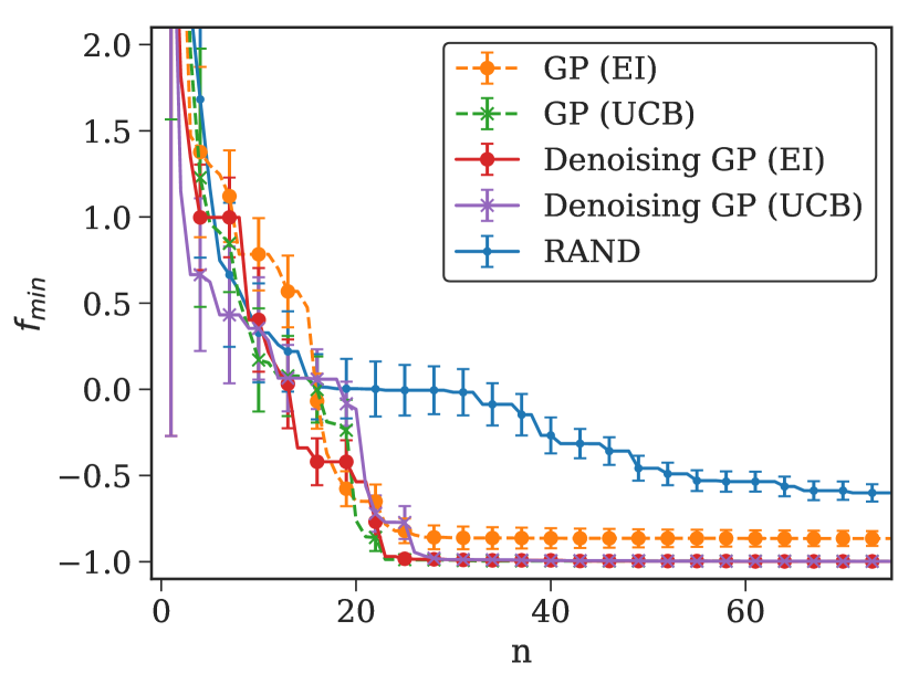
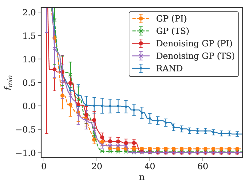
(g) EI and UCB ($p=.33$)

(h) PI and TS ($p=.33$)

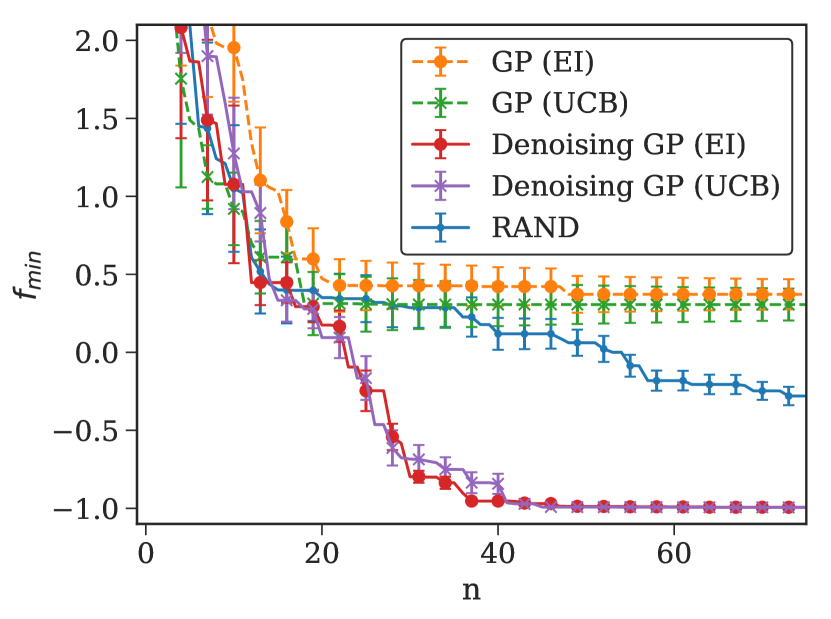
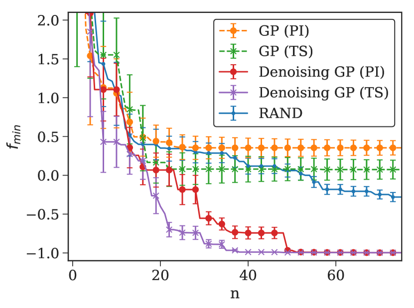
Figure 3. Contaminated BO (Sec. 3.2). We show (a) inference in a GP with n=20 and (b) n=50, and (c)-(d) inference in a denoising GP. In (e)-(f), for low corruption ($p=.01$), ProBO using denoising GPs is competitive with standard BO using GP models. In (g)-(h), for higher corruption ($p=.33$), ProBO converges to the optimal value while standard BO does not. Curves are averaged over 10 trials, and error bars represent one standard error.

BO with Prior Structure on the Objective Function

(a) GP

(b) Basin model

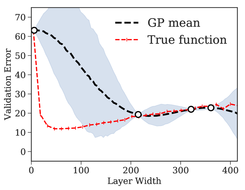
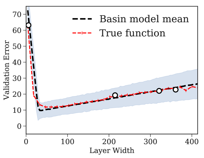
(c) EI and UCB

(d) PI and TS

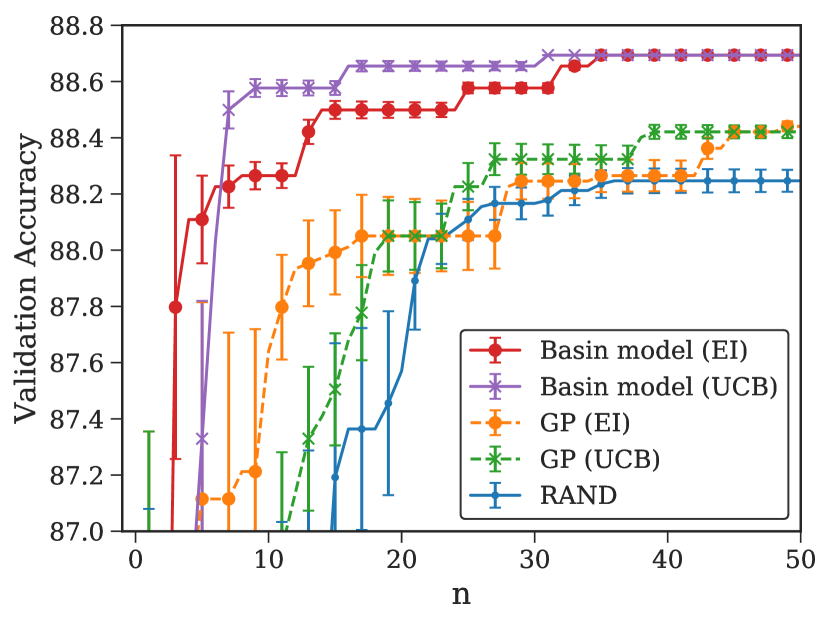
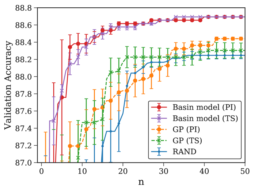
Figure 4. Basin model for overfitting (Sec. 3.3). We plot validation accuracy vs layer width for a small dataset, and show inference in (a) a GP and (b) our basin model. In (c-d) we show results of model complexity hyperparameter tuning experiments, comparing ProBO using a basin model with BO using GPs. Curves are averaged over 10 trials, and error bars represent one standard error.

3.2. Robust Models for Contaminated BO

Setting:

We may want to optimize a system that periodically yields “contaminated observations,” i.e. outliers drawn from a second noise distribution. Examples of this are queries involving unstable simulations [29], or faulty computer systems [41]. This is similar to the setting of Huber’s $\epsilon$-contamination model [19], and we refer to this as contaminated BO. The contaminating distribution may have some dependence on input $\mathcal{X}$ (e.g. may be more prevalent in a window around the optimum value $x^{*}$). Note that this differs from Sec. 3.1 because we do not have access to state observations, and the noise distributions are not in exclusive regions of $\mathcal{X}$. To perform accurate BO in this setting, we need models that are robust to the contamination noise.

Model:

We develop a denoising model, which infers (and ignores) contaminated data points. Given a system model $M_{s}$ and contamination model $M_{c}$ we write our denoising model as $y\sim w_{s}M_{s}(\cdot|z_{s};x)+w_{c}M_{c}(\cdot|z_{c};x)$, where $z_{s},z_{c}\sim\text{Prior}(\cdot)$, and $w_{s},w_{c}\sim\text{Prior}(\cdot|x)$ (and where Prior denotes some appropriate prior density). This is a mixture where weights $(w_{s},w_{c})$ can depend on input $x$. We show inference in this model in Fig. 3 (c)-(d).

Empirical Results:

We show experimental results for ProBO on a synthetic optimization task. This allows us to know the true optimal value $x^{*}$ and objective $f(s(x^{*}))$, which may be difficult to judge in real settings (given the contaminations), and to show results under different contamination levels. For an $x\in\mathbb{R}^{d}$, with probability $1-p$ we query the function $f(x)$ $=$ $\left\lVert x\right\rVert_{2}-\frac{1}{d}\sum_{i=1}^{d}\text{cos}(x_{i})$, which has a minimum value of $f(x^{*})=-1$ at $x^{*}=0_{d}$, and with probability $p$, we receive a contaminated value with distribution $f(x)$ $\sim$ $\text{Unif}([f_{\text{max}}/10,f_{\text{max}}])$, where $f_{\text{max}}$ is $\max_{x\in\mathcal{X}}f(x)$. We compare ProBO using a denoising GP model with standard BO using GPs. We show results for both a low contamination setting $(p=.01)$ and a high contamination setting $(p=.33)$, in Fig. 3 (e)-(h), where we plot the minimal found value (under the noncontaminated model) $f_{\min}$ $=$ $\min_{t\leq n}f(y_{t})$ vs iteration $n$, averaged over 10 trials. In the low contamination setting, both models converge to a near-optimal value and perform similarly, while in the high contamination setting, ProBO with denoising GP converges to a near optimal value while standard BO with GPs does not.

3.3. BO with Prior Structure on the Objective Function

Setting:

In some cases, we have prior knowledge about properties of the objective function, such as trends with respect to $x\in\mathcal{X}$. For example, consider the task of tuning hyperparameters of a machine learning model, where the hyperparameters correspond with model complexity. For datasets of moderate size, there are often two distinct phases as model complexity grows: a phase where the model underfits, where increasing modeling complexity reduces error on a held-out validation set; and a phase where the model overfits, where validation error increases with respect to model complexity. We can design a model that leverages trends such as these.

Model:

We design a model for tuning model complexity, which we refer to as a basin model. Let $y\sim\mathcal{N}(R(x-\mu;a,b)+c,\sigma^{2})$ where $R(x;a,b)$ $=$ $a^{T}\text{ReLU}(x)+b^{T}\text{ReLU}(-x)$, with priors on parameters $\mu\in\mathbb{R}_{d}$, $a,b\in\mathbb{R}_{d}^{+}$, $c\in\mathbb{R}$, and $\sigma^{2}>0$. This model captures the inflection point with variable $\mu$, and uses variables $a$ and $b$ to model the slope of the optimization landscape above and below (respectively) $\mu$. We give a one dimensional view of validation error data from an example where $x$ corresponds to neural network layer width, and show inference with a basin model for this data in Fig. 4 (b).

Empirical Results:

In this experiment, we optimize over the number of units (i.e. layer width) of the hidden layers in a four layer MLP trained on the Wisconsin Breast Cancer Diagnosis dataset [6]. We compare ProBO using a basin model, with standard BO using a GP. We see in Fig 4 (c)-(d) that ProBO with the basin model can significantly outperform standard BO with GPs. In this optimization task, the landscape around the inflection point (of under to over fitting) can be very steep, which may hurt the performance of GP models. In contrast, the basin model can capture this shape and quickly identify the inflection point via inferences about $\mu$.

Structured Multi-task BO

(a) GP (two task) (b) Warp model (two task) (c) EI

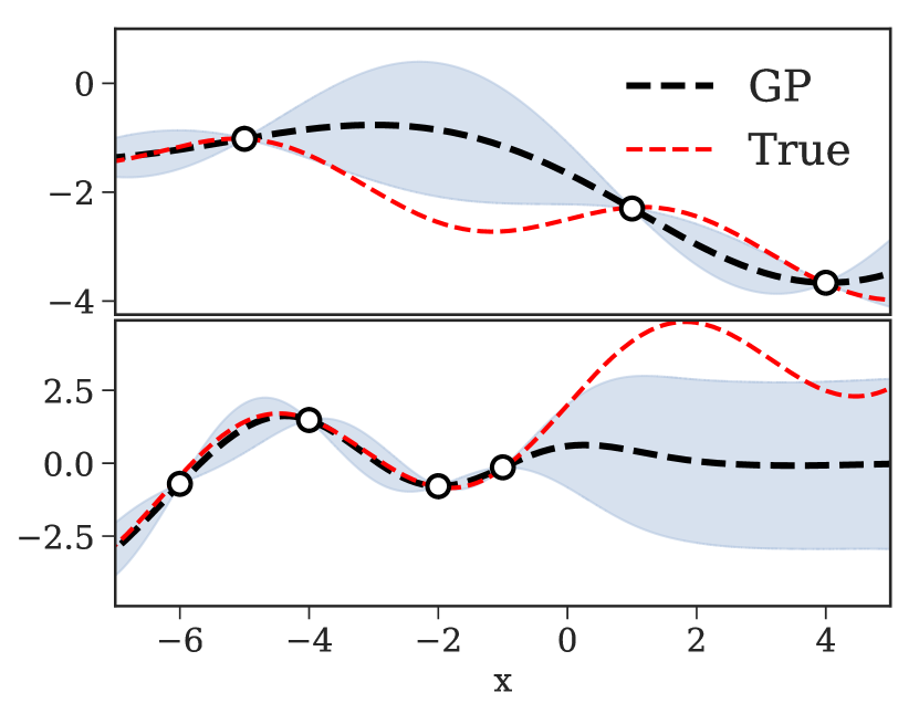
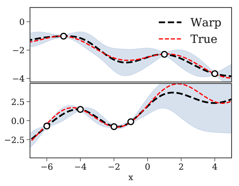
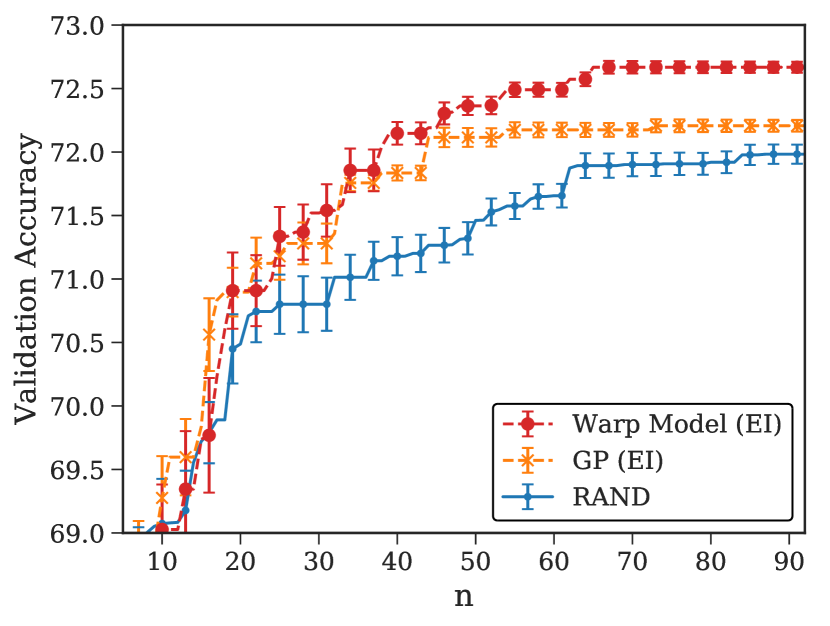
Figure 5. Structured multi-task BO (Sec. 3.4). We show (a) independent GPs and (b) our warp model, in a two-task setting (task one on top, task two on bottom). In (c) we show results for structured multi-task BO on a neural network hyperparameter search problem (details in Appendix Sec. ProBO: Versatile Bayesian Optimization Using Any Probabilistic Programming Language). Curves are averaged over 10 trials, and error bars represent one standard error.

Multi-fidelity Acquisition Functions

(a) EI (b) UCB (c) Calls to gen

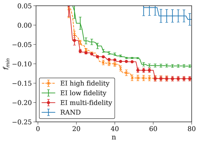
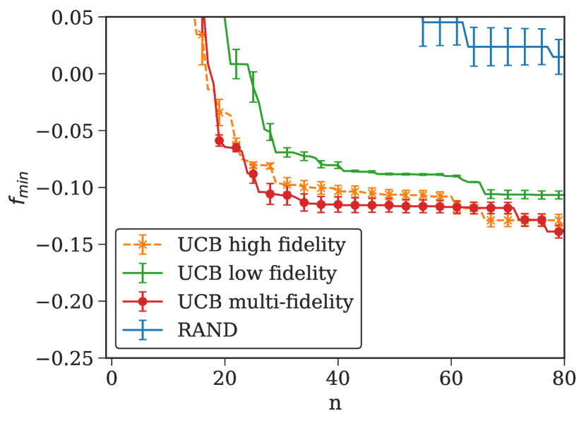
Figure 6. Results on $a_{\text{MF}}$ experiments (Sec. 3.5), showing (a)-(b) ProBO using $a_{\text{MF}}$ (Alg. 6) vs using a fixed high-fidelity $a$ ($M=1000$) and a fixed low-fidelity $a$ ($M=10$). Here, $a_{\text{MF}}$ performs competitively with the high-fidelity $a$, while low fidelity $a$ performs worse. In (c) we show the average number of post/gen calls per evaluation of $a$. We see that the $a_{\text{MF}}$ reduces the number of calls. Curves are averaged over 10 trials, and error bars represent one standard error.

3.4. Structured Models for Multi-task and Contextual BO, and Model Ensembles

We may want to optimize multiple systems jointly, where there is some known relation between the systems. In some instances, we have a finite set of systems (multi-task BO) and in some cases systems are each indexed by a context vector $c\in\mathbb{R}^{d}$ (contextual BO). We develop a model that can incorporate prior structure about the relationship among these systems. Our model warps a latent model based on context/task-specific parameters, so we call this a warp model. We show inference in this model in Fig. 5 (b). In Appendix Sec. ProBO: Versatile Bayesian Optimization Using Any Probabilistic Programming Language we define this model, and describe experimental results shown in Fig. 5 (c).

Alternatively, we may have multiple models that capture different aspects of a system, or we may want to incorporate information given by, for instance, a parametric model (e.g. a model with a specific trend, shape, or specialty for a subset of the data) into a nonparametric model (e.g. a GP, which is highly flexible, but has fewer assumptions). To incorporate multiple sources of information or bring in side information, we want a valid way to create ensembles of multiple PPL models. We develop strategies to combine the posterior predictive densities of multiple PPL models, using only our three PPL operations. We describe this in Appendix Sec. .1.

3.5. Multi-fidelity Acquisition Optimization

We empirically assess our multi-fidelity acquisition function optimization algorithm (Sec. 2.5). Our goal is to demonstrate that increasing the fidelity $M$ in black box acquisitions can yield better performance in ProBO, and that our multi-fidelity method (Alg. 6) maintains the performance of the high-fidelity acquisitions while reducing the number of calls to post and gen. We perform an experiment in a two-fidelity setting, where $M\in\{10,1000\}$, and we apply $a_{\text{MF}}$ to EI and UCB, using a GP model and the (non-corrupted) synthetic system described in Sec. 3.2. Results are shown in Fig. 6 (a)-(c), where we compare high-fidelity $a$ ($M=1000$), low-fidelity $a$ ($M=10$), and multi-fidelity $a_{\text{MF}}$, for EI and UCB acquisitions. For both, the high-fidelity and multi-fidelity methods show comparable performance, while the low-fidelity method performs worse. We also see in Fig. 6 (c) that the multi-fidelity method reduces the number of calls to post/gen by a factor of 3, on average, relative to the high fidelity method.

4. Conclusion

In this paper we presented ProBO, a system for performing Bayesian optimization using models from any probabilistic programming language. We developed algorithms to compute acquisition functions using common PPL operations (without requiring model-specific derivations), and showed how to efficiently optimize these functions. We presented a few models for challenging optimization scenarios, and we demonstrated promising empirical results on the tasks of BO with state observations, contaminated BO, BO with prior structure on the objective function, and structured multi-task BO, where we were able to drop-in models from existing PPL implementations.

• Structured Models for Multi-task and Contextual BO

  In this section we provide details about our models for multi-task and contextual BO, described in Sec. 3.4 and shown in Fig. 5. Many prior methods have been proposed for for multi-task BO [47] and contextual BO [25], though these often focus on new acquisition strategies for GP models. Here we propose a model for the case where we have some structured prior information about the relation between systems, or some parametric relationship that we want to incorporate into our model.

  We first consider the multi-task setting and then extend this to the contextual setting. Suppose that we have $T$ tasks (i.e. subsystems to optimize) with data subsets $\mathcal{D}$ $=$ $\left\{\mathcal{D}_{1},\ldots,\mathcal{D}_{T}\right\}$, where $\mathcal{D}_{t}$ has data $\{x_{t,i},y_{t,i}\}_{i=1}^{n_{t}}$, and where $n_{t}$ denotes the number of observations in the $t^{\text{th}}$ task. For each $(x_{t,i},y_{t,i})$ pair within $\mathcal{D}$, we have a latent variable $z_{t,i}\in\mathcal{Z}$. Additionally, for each task $t$, we have task-specific latent “warp” variables, denoted $w_{t}$.

  Given these, we define our warp model to be

  1. For $t=1,\ldots,T$:

     1. $w_{t}\sim\text{Prior}(w)$

     2. For $i=1,\ldots,n_{t}$:

        1. $z_{t,i}\sim p(z|x_{t,i})$

        2. $y_{t,i}\sim p(y|z_{t,i},x_{t,i},w_{t})$

  We call $p(z|x_{t,i})$ our latent model, and $p(y|z_{t,i},x_{t,i},w_{t})$ our warp model, which is parameterized by warp variables $w_{t}$. Intuitively, we can think of the variables $z_{t,i}$ as latent “unwarped” versions of observations $y_{t,i}$, all in a single task. Likewise, we can intuitively think of observed variables $y_{t,i}$ as “warped versions of $z_{t,i}$”, where $w_{t}$ dictates the warping for each subset of data $\mathcal{D}_{t}$.

  Task 1 ($n_{1}=7$)

  Task 2 ($n_{2}=5$)

  

  

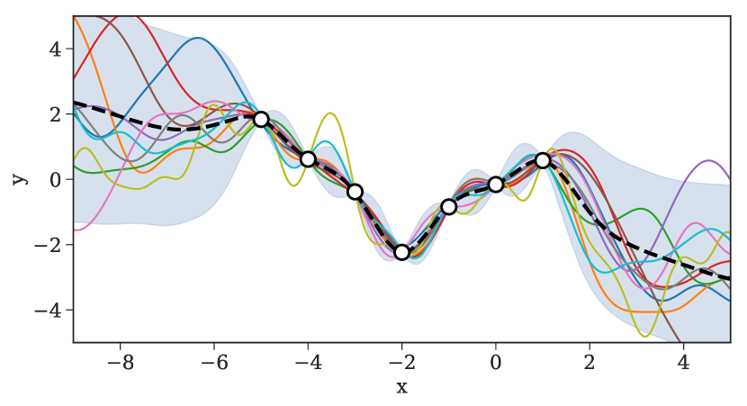
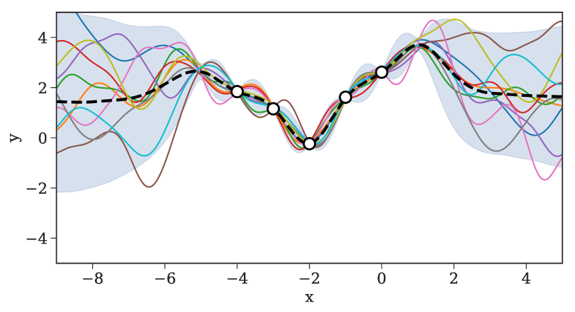
  Figure 7. Warp model inference on tasks one (left) and two (right), where $n_{1}=7$ and $n_{2}=5$. This warp model assumes a linear warp with respect to both the latent variables $z$ and inputs $x$. Posterior mean, posterior samples, and posterior predictive distribution are shown.

  Task 1 ($n_{1}=7$)

  Task 2 ($n_{2}=3$)

  

  

  Figure 8. Warp model inference on tasks one (left) and two (right), where $n_{1}=7$ and $n_{2}$ is reduced to $n_{2}=3$. This warp model assumes a linear warp with respect to both the latent variables $z$ and inputs $x$. Posterior mean, posterior samples, and posterior predictive distribution are shown. Here, we see more uncertainty around the two removed points in task two, relative to Fig. 7.

  We now give a concrete instantiation of this model. Let the latent model be $p(z|x_{t,i})$ $=$ $\mathcal{GP}\left(\mu(x),k(x,x^{\prime})\right)$, i.e. we put a Gaussian process prior on the latent variables $z$. For a given task, let the warping model for $y$ be a linear function of both $z$ and $x$ (with some added noise), where warping parameters $w$ are parameters of this linear model, i.e. $y_{t,i}\sim w_{0}+w_{1}x_{t,i}+w_{2}z_{t,i}+\epsilon$.

  Intuitively, this model assumes that there is a latent GP, which is warped via a linear model of both the GP output $z$ and input $x$ to yield observations $y$ for a given task (and that there is a separate warp for each task). We illustrate this model in Fig. 7 and 8 (where $n_{1}=7$ in both, $n_{2}=5$ in the former, and $n_{2}=3$ in the latter). As we remove points $x$ in task two, we see more uncertainty in the posterior predictive distribution at these points.

  We can also extend this warp model for use in a contextual optimization setting, where we want to jointly optimize over a set of systems each indexed by a context vector $c\in\mathbb{R}^{d}$. In practice, we observe the context $c_{i}$ for input $x_{i}\in\mathcal{X}$, and therefore perform inference on a dataset $\mathcal{D}_{n}=\{x_{i},c_{i},y_{i}\}_{i=1}^{n}$.

  To allow for this, we simply let our warp model also depend on $c$, i.e. let the warp model be $p(y|z_{t,i},x_{t,i},w_{t},c_{t,i})$. Intuitively, this model assumes that there is a single latent system, which is warped by various factors (e.g. the context variables) to produce observations.

  .1. Empirical Results

  Here we describe the empirical results shown in Fig. 5 (c). We aim to perform the neural architecture and hyperparameter search task from Sec. 3.1, but for two different settings, each with a unique preset batch size. Based on prior observations, we believe that the validation accuracy of both systems at a given query $x$ can be accurately modeled as a linear transformation of some common latent system, and we apply the warp model described above. We compare ProBO using this warp model with a single GP model over the full space of tasks and inputs. We show results in Fig. 5 (c), where we plot the best validation accuracy found over both tasks vs iteration $n$. Both methods use the EI acquisition function, and we compare these against a baseline that chooses queries uniformly at random. Here, ProBO with the warp model is able to find a query with a better maximum validation accuracy, relative to standard BO with GP model. Ensembles of PPL Models within ProBO

  We may have multiple models that capture different aspects of a system, or we may want to incorporate information given by, for instance, a parametric PPL model (e.g. a model with a specific trend, shape, or specialty for a subset of the data) into a nonparametric PPL model (e.g. a GP, which is flexible, but has fewer assumptions).

  To incorporate multiple sources of information or bring in side information, we want a valid way to create ensembles of multiple models. Here, we develop a method to combine the posterior predictive densities of multiple PPL models, using only our three PPL operations. Our procedure constructs a model similar to a product of experts model [17], and we call our strategy a Bayesian product of experts (BPoE). This model can then be used in our ProBO framework.

  As an example, we show an ensemble of two models, $\mathcal{M}_{1}$ and $\mathcal{M}_{2}$, though this could be extended to an arbitrarily large group of models. Assume $\mathcal{M}_{1}$ and $\mathcal{M}_{2}$ are both plausible models for a dataset $\mathcal{D}_{n}=\{(x_{i},y_{i})\}_{i=1}^{n}$.

  Let $\mathcal{M}_{1}$ have likelihood $p_{1}(\mathcal{D}_{n}|z_{1})$ $=$ $\prod_{i=1}^{n}p_{1}(y_{i}|z_{1};x_{i})$, where $z_{1}\in\mathcal{Z}_{1}$ are latent variables with prior $p_{1}(z_{1})$. We define the joint model PDF for $\mathcal{M}_{1}$ to be $p_{1}(\mathcal{D}_{n},z_{1})$ $=$ $p_{1}(z_{1})\prod_{i=1}^{n}p_{1}(y_{i}|z_{1};x_{i})$. The posterior (conditional) PDF for $\mathcal{M}_{1}$ can then be written $p_{1}(z_{1}|\mathcal{D}_{n})=p_{1}(\mathcal{D}_{n},z_{1})/p_{1}(\mathcal{D}_{n})$. We can write the posterior predictive PDF for $\mathcal{M}_{1}$ as

  $$p_{1}(y|\mathcal{D}_{n};x)=\mathbb{E}_{p_{1}(z_{1}|\mathcal{D}_{n})}\left[p_{1}(y|z_{1};x)\right].$$ (.1)

  Similarly, let $\mathcal{M}_{2}$ have likelihood $p_{2}(\mathcal{D}_{n}|z_{2})$ $=$ $\prod_{i=1}^{n}p_{2}(y_{i}|z_{2};x_{i})$, where $z_{2}\in\mathcal{Z}_{2}$ are latent variables with prior PDF $p_{2}(z_{2})$. We define the joint model PDF for $\mathcal{M}_{2}$ to be $p_{2}(\mathcal{D}_{n},z_{2})$ $=$ $p_{2}(z_{2})\prod_{i=1}^{n}p_{2}(y_{i}|z_{2};x_{i})$, the posterior (conditional) PDF to be $p_{2}(z_{2}|\mathcal{D}_{n})$ $=$ $p_{2}(\mathcal{D}_{n},z_{2})/p_{2}(\mathcal{D}_{n})$, and the posterior predictive PDF to be

  $$p_{2}(y|\mathcal{D}_{n};x)=\mathbb{E}_{p_{2}(z_{2}|\mathcal{D}_{n})}\left[p_{2}(y|z_{2};x)\right].$$ (.2)

  Note that $z_{1}\in\mathcal{Z}_{1}$ and $z_{2}\in\mathcal{Z}_{2}$ need not be in the same space nor related.

  Given models $\mathcal{M}_{1}$ and $\mathcal{M}_{2}$, we define the Bayesian Product of Experts (BPoE) ensemble model, $\mathcal{M}_{e}$, with latent variables $z=(z_{1},z_{2})\in\mathcal{Z}_{1}\times\mathcal{Z}_{2}$, to be the model with posterior predictive density

  $$p(y|\mathcal{D}_{n};x)\propto p_{1}(y|\mathcal{D}_{n};x)p_{2}(y|\mathcal{D}_{n};x).$$ (.3)

  The posterior predictive PDF for the BPoE ensemble model $\mathcal{M}_{e}$ is proportional to the product of the posterior predictive PDFs of the constituent models $\mathcal{M}_{1}$ and $\mathcal{M}_{2}$. Note that this uses the product of expert assumption [17] on $y$, which intuitively means that $p(y|\mathcal{D}_{n};x)$ is high where both $p_{1}(y|\mathcal{D}_{n};x)$ and $p_{2}(y|\mathcal{D}_{n};x)$ agree (i.e. an “and” operation). Intuitively, this model gives a stronger posterior belief over $y$ in regions where both models have consensus, and weaker posterior belief over $y$ in regions given by only one (or neither) of the models.

  Given this model, we need an algorithm for computing and using the posterior predictive for $\mathcal{M}_{e}$ within the ProBO framework. In our acquisition algorithms, we use gen to generate samples from predictive distributions. We can integrate these with combination algorithms from the embarrassingly parallel MCMC literature [35, 52, 36] to develop an algorithm that generates samples from the posterior predictive of the ensemble model $\mathcal{M}_{e}$ and uses these in a new acquisition algorithm. We give this procedure in Alg. 8, which introduces the ensemble operation. Note that ensemble takes as input two operations gen1 and gen2 (assumed to be from two PPL models), as well as two sets of $M$ posterior samples $z_{1}^{M}$ and $z_{2}^{M}$ (assumed to come from calls to post1 and post2 from the two PPL models). Also note that in Alg. 8 we’ve used $\text{Combine}(y_{1},y_{2})$ to denote a combination algorithm, which we detail in appendix Sec. .3.

  We can now swap the ensemble operation in for the gen operation in Algs. 2-5. Note that the BPoE allows us to easily ensemble models written in different PPLs. For example, a hierarchical regression model written in Stan [7] using Hamiltonian Monte Carlo for inference could be combined with a deep Bayesian neural network written in Pyro [5] using variational inference and with a GP written in GPy [14] using exact inference.

  Algorithm 8   ensemble$(x,\texttt{gen1},$ $\texttt{gen2},z_{1}^{M},z_{2}^{M})$ $\triangleright$ PPL model ensemble with BPoE

  1:for $m=1,\ldots,M$ do

  2:     $s_{1},s_{2}\sim\text{Unif}\left(\{1,\ldots,M\}\right)$

  3:     $\tilde{y}_{1,m}\leftarrow\texttt{gen1}(x,z_{1,s_{1}},s_{1})$

  4:     $\tilde{y}_{2,m}\leftarrow\texttt{gen2}(x,z_{2,s_{2}},s_{2})$

  5:$y_{1:M}\leftarrow\text{Combine}(\tilde{y}_{1,M},\tilde{y}_{2,M})$

  6:Return $y_{1:M}$.

  .2. Example: Combining Phase-Shift and GP Models.

  We describe an example and illustrate it in Fig. 9. Suppose we expect a few phase shifts in our input space $\mathcal{X}$, which partition $\mathcal{X}$ into regions with uniform output. We can model this system with $y$ $\sim$ $\mathcal{N}(y|\sum_{k=1}^{K}\text{logistic}(x;m_{k},s_{k},\mu_{k})+b_{k},\sigma^{2})$, where latent variables $m_{1:K}$, $s_{1:K}$, $\mu_{1:K}$, and $b_{1:K}$ are assigned appropriate priors, and where $\text{logistic}(x;m,s,\mu)$ $=$ $\frac{m}{1+\exp(-s(x-\mu))}$. This model may accurately describe general trends in the system, but it may be ultimately misspecified, and underfit as the number of observations $n$ grows.

  Alternatively, we could model this system as a black box using a Gaussian process. The GP posterior predictive may converge to the correct landscape given enough data, but it is nonparametric, and does not encode our assumptions.

  We can use the BPoE model to combine both the phase shift and GP models. We see in Fig. 9 that when $n=2$ (first row), the BPoE model resembles the phase shift model, but when $n=50$ (second row), it more closely resembles the true landscape modeled by the GP.

  Phase Shift (PS) Model     Gaussian Process (GP) BPoE Ensemble (PS, GP)

        $n$ = 2

  

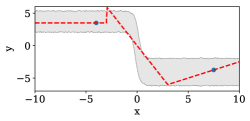
  (a)

  

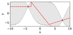
  (b)

  

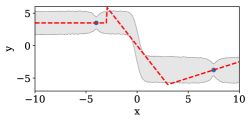
  (c)

        $n$ = 50

  

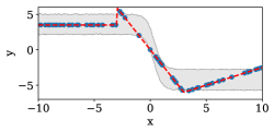
  (d)

  

  (e)

  

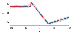
  (f)

  Figure 9. Visualization of the Bayesian product of experts (BPoE) ensemble model (column 3) of a phase shift (PS) model (column 1), defined in Sec. .2, and a GP (column two). In the first row ($n=2$), when $n$ is small, the BPoE ensemble more closely resembles the PS model. In the second row ($n=50$), when $n$ is larger, the BPoE ensemble more closely resembles the GP model, and both accurately reflect the true landscape (red dashed line). In all figures, the posterior predictive is shown in gray.

  .3. Combination Algorithms for the ensemble Operation (Alg. 8)

  We make use of combination algorithms from the embarrassingly parallel MCMC literature [35, 52, 36], to define the ensemble operation (Alg. 8) for use in applying the ProBO framework to a BPoE model. We describe these combination algorithms here in more detail.

  For convenience, we describe these methods for two Bayesian models, $\mathcal{M}_{1}$ and $\mathcal{M}_{2}$, though these methods apply similarly to an abitrarily large set of models.

  The goal of these combination methods is to combine a set of $M$ samples $y_{1,1:M}\sim p_{1}(y|\mathcal{D}_{n};x)$ from the posterior predictive distribution of a model $\mathcal{M}_{1}$, with a disjoint set of $M$ samples $y_{2,1:M}\sim p_{2}(y|\mathcal{D}_{n};x)$ from the posterior predictive distribution of a model $\mathcal{M}_{2}$, to produce samples

  $$y_{3,1:M}\sim p(y|\mathcal{D}_{n};x)\propto p_{1}(y|\mathcal{D}_{n};x)p_{2}(y|\mathcal{D}_{n};x),$$ (.4)

  where $p(y|\mathcal{D}_{n};x)$ denotes the posterior predictive distribution of a BPoE ensemble model $\mathcal{M}_{e}$, with constituent models $\mathcal{M}_{1}$ and $\mathcal{M}_{2}$.

  We use the notation $\text{Combine}(y_{1,1:M},y_{2,1:M})$ to denote a combination algorithm. We give a combination algorithm in Alg. 9 for our setting based on a combination algorithm presented in [35].

  Algorithm 9   $\text{Combine}(y_{1,1:M},y_{2,1:M}))$ $\triangleright$ Combine sample sets

  1:$t_{1},t_{2}\overset{\text{iid}}{\sim}\text{Unif}\left(\{1,\ldots,M\}\right)$

  2:for $i=1,\ldots,M$ do

  3:     $c_{1},c_{2}\overset{\text{iid}}{\sim}\text{Unif}\left(\{1,\ldots,M\}\right)$

  4:     $u\sim\text{Unif}\left([0,1]\right)$

  5:     if $u>\frac{w_{(c_{1},c_{2})}}{w_{(t_{1},t_{2})}}$ then

  6:         $t_{1}\leftarrow c_{1}$

  7:         $t_{2}\leftarrow c_{2}$      

  8:     $y_{3,i}\sim\mathcal{N}\left(\bar{y}_{(t_{1},t_{2})},\frac{i^{-1/2}}{2}\right)$

  9:Return $y_{3,1:M}$.

  We must define a couple of terms used in Alg. 9. The mean output $\bar{y}_{(t_{1},t_{2})}$, for indices $t_{1},t_{2}\in\{1,\ldots,M\}$, is defined to be

  $$\bar{y}_{(t_{1},t_{2})}=\frac{1}{2}\left(y_{1,t_{1}}+y_{2,t_{2}}\right),$$ (.5)

  and weights $w_{(t_{1},t_{2})}$ (alternatively, $w_{(c_{1},c_{2})}$), for indices $t_{1},t_{2}\in\{1,\ldots,M\}$, are defined to be

  $$w_{(t_{1},t_{2})}=\mathcal{N}\left(y_{1,t_{1}}|\bar{y}_{(t_{1},t_{2})},i^{-1/2}\right)\mathcal{N}\left(y_{2,t_{2}}|\bar{y}_{(t_{1},t_{2})},i^{-1/2}\right).$$ (.6)

  Note that this $\text{Combine}(y_{1,1:M},y_{2,1:M})$ algorithm (Alg. 9) holds for sample sets from two arbitrary posterior predictive distributions $p_{1}(y|\mathcal{D}_{n};x)$ and $p_{2}(y|\mathcal{D}_{n};x)$, without any parametric assumptions such as Gaussianity.

References

- [1] Omid Alipourfard, Hongqiang Harry Liu, Jianshu Chen, Shivaram Venkataraman, Minlan Yu, and Ming Zhang, Cherrypick: Adaptively unearthing the best cloud configurations for big data analytics, 14th USENIX Symposium on Networked Systems Design and Implementation (NSDI 17), 2017, pp. 469–482.
- [2] S. Ambikasaran, D. Foreman-Mackey, L. Greengard, D. W. Hogg, and M. O’Neil, Fast Direct Methods for Gaussian Processes and the Analysis of NASA Kepler Mission Data, (2014).
- [3] Raul Astudillo and P Frazier, Multi-attribute bayesian optimization under utility uncertainty, Proceedings of the NIPS Workshop on Bayesian Optimization, 2017.
- [4] Rémi Bardenet, Arnaud Doucet, and Chris Holmes, On markov chain monte carlo methods for tall data, The Journal of Machine Learning Research 18 (2017), no. 1, 1515–1557.
- [5] Eli Bingham, Jonathan P. Chen, Martin Jankowiak, Fritz Obermeyer, Neeraj Pradhan, Theofanis Karaletsos, Rohit Singh, Paul Szerlip, Paul Horsfall, and Noah D. Goodman, Pyro: Deep Universal Probabilistic Programming, Journal of Machine Learning Research (2018).
- [6] CL Blake and CJ Merz, Uci repository of machine learning databases. irvine, ca: University of california, department of information and computer science, 1998.
- [7] Bob Carpenter, Andrew Gelman, Matt Hoffman, Daniel Lee, Ben Goodrich, Michael Betancourt, Marcus A Brubaker, Jiqiang Guo, Peter Li, and Allen Riddell, Stan: a probabilistic programming language, Journal of Statistical Software (2015).
- [8] Valentin Dalibard, Michael Schaarschmidt, and Eiko Yoneki, Boat: Building auto-tuners with structured bayesian optimization, Proceedings of the 26th International Conference on World Wide Web, International World Wide Web Conferences Steering Committee, 2017, pp. 479–488.
- [9] Joshua V Dillon, Ian Langmore, Dustin Tran, Eugene Brevdo, Srinivas Vasudevan, Dave Moore, Brian Patton, Alex Alemi, Matt Hoffman, and Rif A Saurous, Tensorflow distributions, arXiv preprint arXiv:1711.10604 (2017).
- [10] Bradley Efron, Bootstrap methods: another look at the jackknife, Breakthroughs in statistics, Springer, 1992, pp. 569–593.
- [11] Alexander IJ Forrester, András Sóbester, and Andy J Keane, Multi-fidelity optimization via surrogate modelling, Proceedings of the royal society of london a: mathematical, physical and engineering sciences, vol. 463, The Royal Society, 2007, pp. 3251–3269.
- [12] Jacob R Gardner, Matt J Kusner, Zhixiang Eddie Xu, Kilian Q Weinberger, and John P Cunningham, Bayesian optimization with inequality constraints, ICML, 2014, pp. 937–945.
- [13] Michael A Gelbart, Jasper Snoek, and Ryan P Adams, Bayesian optimization with unknown constraints, arXiv preprint arXiv:1403.5607 (2014).
- [14] GPy, GPy: A gaussian process framework in python, http://github.com/SheffieldML/GPy, 2012.
- [15] Philipp Hennig and Christian J Schuler, Entropy search for information-efficient global optimization, Journal of Machine Learning Research 13 (2012), no. Jun, 1809–1837.
- [16] José Miguel Hernández-Lobato, Michael A Gelbart, Matthew W Hoffman, Ryan P Adams, and Zoubin Ghahramani, Predictive entropy search for bayesian optimization with unknown constraints, (2015).
- [17] Geoffrey E Hinton, Training products of experts by minimizing contrastive divergence, Neural computation 14 (2002), no. 8, 1771–1800.
- [18] Matthew D Hoffman and Andrew Gelman, The no-u-turn sampler: Adaptively setting path lengths in hamiltonian monte carlo, arXiv preprint arXiv:1111.4246 (2011).
- [19] Peter J Huber, Robust estimation of a location parameter, Breakthroughs in statistics, Springer, 1992, pp. 492–518.
- [20] Ferenc Huszár, Variational inference using implicit distributions, arXiv preprint arXiv:1702.08235 (2017).
- [21] Frank Hutter, Holger H Hoos, and Kevin Leyton-Brown, Sequential model-based optimization for general algorithm configuration, International Conference on Learning and Intelligent Optimization, Springer, 2011, pp. 507–523.
- [22] Pasi Jylänki, Jarno Vanhatalo, and Aki Vehtari, Robust gaussian process regression with a student-t likelihood, Journal of Machine Learning Research 12 (2011), no. Nov, 3227–3257.
- [23] Kirthevasan Kandasamy, Willie Neiswanger, Jeff Schneider, Barnabas Poczos, and Eric Xing, Neural architecture search with bayesian optimisation and optimal transport, arXiv preprint arXiv:1802.07191 (2018).
- [24] Diederik P Kingma and Max Welling, Auto-encoding variational bayes, arXiv preprint arXiv:1312.6114 (2013).
- [25] Andreas Krause and Cheng S Ong, Contextual gaussian process bandit optimization, Advances in Neural Information Processing Systems, 2011, pp. 2447–2455.
- [26] Harold J Kushner, A new method of locating the maximum point of an arbitrary multipeak curve in the presence of noise, Journal of Basic Engineering 86 (1964), no. 1, 97–106.
- [27] Remi Lam and Karen Willcox, Lookahead bayesian optimization with inequality constraints, Advances in Neural Information Processing Systems, 2017, pp. 1890–1900.
- [28] Tuan Anh Le, Atilim Gunes Baydin, and Frank Wood, Inference compilation and universal probabilistic programming, arXiv preprint arXiv:1610.09900 (2016).
- [29] DD Lucas, R Klein, J Tannahill, D Ivanova, S Brandon, D Domyancic, and Y Zhang, Failure analysis of parameter-induced simulation crashes in climate models, Geoscientific Model Development 6 (2013), no. 4, 1157–1171.
- [30] David J Lunn, Andrew Thomas, Nicky Best, and David Spiegelhalter, Winbugs-a bayesian modelling framework: concepts, structure, and extensibility, Statistics and computing 10 (2000), no. 4, 325–337.
- [31] Vikash Mansinghka, Daniel Selsam, and Yura Perov, Venture: a higher-order probabilistic programming platform with programmable inference, arXiv preprint arXiv:1404.0099 (2014).
- [32] Vikash K Mansinghka, Tejas D Kulkarni, Yura N Perov, and Josh Tenenbaum, Approximate bayesian image interpretation using generative probabilistic graphics programs, Advances in Neural Information Processing Systems, 2013, pp. 1520–1528.
- [33] Tom Minka, Infer. net 2.5, http://research. microsoft. com/infernet (2012).
- [34] Jonas Močkus, On bayesian methods for seeking the extremum, Optimization Techniques IFIP Technical Conference, Springer, 1975, pp. 400–404.
- [35] Willie Neiswanger, Chong Wang, and Eric Xing, Asymptotically exact, embarrassingly parallel mcmc, Proceedings of the 30th Conference on Uncertainty in Artificial Intelligence (UAI 2014), 2014.
- [36] Willie Neiswanger and Eric Xing, Post-inference prior swapping, Proceedings of the 34th International Conference on Machine Learning-Volume 70, JMLR. org, 2017, pp. 2594–2602.
- [37] Tom Rainforth, Tuan Anh Le, Jan-Willem van de Meent, Michael A Osborne, and Frank Wood, Bayesian optimization for probabilistic programs, Advances in Neural Information Processing Systems, 2016, pp. 280–288.
- [38] Rajesh Ranganath, Sean Gerrish, and David Blei, Black box variational inference, Artificial Intelligence and Statistics, 2014, pp. 814–822.
- [39] Daniel Ritchie, Paul Horsfall, and Noah D Goodman, Deep amortized inference for probabilistic programs, arXiv preprint arXiv:1610.05735 (2016).
- [40] John Salvatier, Thomas V Wiecki, and Christopher Fonnesbeck, Probabilistic programming in python using pymc3, PeerJ Computer Science 2 (2016), e55.
- [41] Bianca Schroeder and Garth Gibson, A large-scale study of failures in high-performance computing systems, IEEE transactions on Dependable and Secure Computing 7 (2009), no. 4, 337–350.
- [42] Amar Shah, Andrew Wilson, and Zoubin Ghahramani, Student-t processes as alternatives to gaussian processes, Artificial Intelligence and Statistics, 2014, pp. 877–885.
- [43] Jack W Smith, JE Everhart, WC Dickson, WC Knowler, and RS Johannes, Using the adap learning algorithm to forecast the onset of diabetes mellitus, Proceedings of the Annual Symposium on Computer Application in Medical Care, American Medical Informatics Association, 1988, p. 261.
- [44] Jasper Snoek, Hugo Larochelle, and Ryan P Adams, Practical bayesian optimization of machine learning algorithms, Advances in neural information processing systems, 2012, pp. 2951–2959.
- [45] Jasper Snoek, Oren Rippel, Kevin Swersky, Ryan Kiros, Nadathur Satish, Narayanan Sundaram, Mostofa Patwary, Mr Prabhat, and Ryan Adams, Scalable bayesian optimization using deep neural networks, International Conference on Machine Learning, 2015, pp. 2171–2180.
- [46] Niranjan Srinivas, Andreas Krause, Sham M Kakade, and Matthias Seeger, Gaussian process optimization in the bandit setting: No regret and experimental design, arXiv preprint arXiv:0912.3995 (2009).
- [47] Kevin Swersky, Jasper Snoek, and Ryan P Adams, Multi-task bayesian optimization, Advances in neural information processing systems, 2013, pp. 2004–2012.
- [48] William R Thompson, On the likelihood that one unknown probability exceeds another in view of the evidence of two samples, Biometrika 25 (1933), no. 3/4, 285–294.
- [49] Tina Toni, David Welch, Natalja Strelkowa, Andreas Ipsen, and Michael PH Stumpf, Approximate bayesian computation scheme for parameter inference and model selection in dynamical systems, Journal of the Royal Society Interface 6 (2008), no. 31, 187–202.
- [50] Dustin Tran, Alp Kucukelbir, Adji B. Dieng, Maja Rudolph, Dawen Liang, and David M. Blei, Edward: A library for probabilistic modeling, inference, and criticism, arXiv preprint arXiv:1610.09787 (2016).
- [51] Dustin Tran, Rajesh Ranganath, and David Blei, Hierarchical implicit models and likelihood-free variational inference, Advances in Neural Information Processing Systems, 2017, pp. 5523–5533.
- [52] Xiangyu Wang, Fangjian Guo, Katherine A Heller, and David B Dunson, Parallelizing mcmc with random partition trees, arXiv preprint arXiv:1506.03164 (2015).
- [53] James T Wilson, Frank Hutter, and Marc Peter Deisenroth, Maximizing acquisition functions for bayesian optimization, arXiv preprint arXiv:1805.10196 (2018).
- [54] Frank Wood, Jan Willem van de Meent, and Vikash Mansinghka, A new approach to probabilistic programming inference, Proceedings of the 17th International conference on Artificial Intelligence and Statistics, 2014, pp. 1024–1032.
- [55] Jian Wu, Matthias Poloczek, Andrew G Wilson, and Peter Frazier, Bayesian optimization with gradients, Advances in Neural Information Processing Systems, 2017, pp. 5267–5278.
- [56] Barret Zoph and Quoc V Le, Neural architecture search with reinforcement learning, arXiv preprint arXiv:1611.01578 (2016).
-
\appsection